Shapley Value-Based Payment Calculation for Energy Exchange between Micro- and Utility Grids


1
Graduate Institute of Industrial Engineering, National Taiwan University, Taipei 10617, Taiwan
2
Department of Electrical Engineering, National Taiwan University, Taipei 10617, Taiwan
3
Department of Electrical and Computer Engineering, University of Connecticut, Storrs, CT 06269, USA
*
Author to whom correspondence should be addressed.
Games 2017, 8(4), 45; https://doi.org/10.3390/g8040045
Submission received: 31 July 2017
/
Revised: 2 October 2017
/
Accepted: 11 October 2017
/
Published: 23 October 2017
Abstract
:In recent years, microgrids have developed as important parts of power systems and have provided affordable, reliable, and sustainable supplies of electricity. Each microgrid is managed as a single controllable entity with respect to the existing power system but demands for joint operation and sharing the benefits between a microgrid and its hosting utility. This paper is focused on the joint operation of a microgrid and its hosting utility, which cooperatively minimize daily generation costs through energy exchange, and presents a payment calculation scheme for power transactions based on a fair allocation of reduced generation costs. To fairly compensate for energy exchange between the micro- and utility grids, we adopt the cooperative game theoretic solution concept of Shapley value. We design a case study for a fictitious interconnection model between the Mueller microgrid in Austin, Texas and the utility grid in Taiwan. Our case study shows that when compared to standalone generations, both the micro- and utility grids are better off when they collaborate in power exchange regardless of their individual contributions to the power exchange coalition.
1. Introduction
The integration of changing technologies and new entrants in the generation market requires major changes in the operations of the electricity market to become smarter in order to provide an affordable, reliable, and sustainable supply of electricity [1,2]. To enhance the reliability and reduce the costs of an integrated transmission grid, the smart grid concept has encouraged researchers [3,4,5] to study ways of generating power locally in proximity to the customer through combining together loads and distributed generation (DG) in so called microgrids. A microgrid is a network of small-scale distributed energy resources (DER), such as solar panels, wind turbines, fuel cells, and micro-turbines that can either operate standalone or interconnected to the utility grid. Its feature to be managed as a single controllable entity with respect to the existing power system poses several benefits, and demands for joint operation models with the utility network.
To incentivize collaboration in energy exchange between a microgrid and its hosting utility, however, we analyzed three inter-related design problems that will be addressed in the remainder of this research: the joint operation, cost allocation, and the payment calculation problem.
Therefore, we first analyze the design problems for collaboration in energy exchange, then present a centralized decision model for the joint operation of a microgrid and its hosting utility, and finally suggest a payment calculation scheme that compensates for energy exchange based on fairly allocating joint generation costs. In this regard, we adopt the cooperative game theoretic solution concept of Shapley value to fairly allocate reduced generation costs from joint operation and incentivize generation cost savings that can be realized when the micro- and utility grids form a coalition through mutual payments for energy exchange.
1.1. Joint Operation Problem
According to Hogan [1], the problem of how to jointly deliver an aggregated load schedule involving multiple power grids has initially been discussed for vertically integrated utilities in regulated energy markets. To address the problem, utilities traditionally formed coalitions, e.g., in the form of power pools, to jointly dispatch their generation resources and thereby achieve cost savings. In this regards, Chattopadhyay [6] presents a linear programming (LP) formulation of an energy brokerage system, which maximizes the savings for interconnected utilities participating in a power pool.
Particularly against the background of the benefits that arise from an energy exchange between a microgrid and its extant power system, this is also an issue for the joint operation of a microgrid and its hosting utility. Distributed energy trading concepts help power grids to cooperatively gain and share the benefits through economies of scale and making the best use of all available resources; among others by reducing system operation costs through access to linked generation resources, which may improve generation decisions. An overview of distributed energy trading concepts for microgrids is provided by Bayram et al. [7]. In this context, Asimakopoulou et al. [8] discusses decision models for the interaction between the utility and the microgrid.
As our research cooperatively optimizes energy management between the utility and the microgrid to maximize total cost savings of both power grids, we suggest a centralized decision framework where a centralized planer solves the interaction between the power grids as a single objective maximization problem to jointly optimize available generation units. Since there is only one entity, our joint generation cost model represents the ideal case of adducing an aggregated load schedule without a profit margin for energy exchange and describes the best way to achieve joint cost savings between the micro- and utility grid.
1.2. Cost Allocation Problem
Notwithstanding, a major obstacle for the collaboration in energy exchange still constitutes the application of a cost sharing rule that fairly allocates the potential costs saving benefit from jointly delivering an aggregated load schedule when the networks cooperate as a single unit. In recent years, the theoretical analysis to develop criteria and methods for cost allocation problems emerged as the field of cost sharing games. The methods to define and solve cost sharing games are summarized by Jain et al. [9].
Cost sharing games provide a proper basis to allocate the costs for a group of parties that wants to divide the cost of a common facility or operation. In this regard, each party has a standalone cost if it does not cooperate with the others. Similarly, each subgroup of parties has a shared cost if parties cooperate with each other but not with the remaining parties. Even though cost sharing games allow the assessment of the value of a coalition in the context of a given scenario, they do not solve the problem how the value should be shared. Therefore, a cost sharing rule can help to allocate the total cost among the members of a group for every possible cost sharing game.
To address a common cost allocation problem, several methods have been discussed for the distribution of joint cost and the division of surplus, among others the Shapley value [10]. The Shapley value was introduced by Shapley [11] as a method for players to assess, a priori, their benefits from playing a game and suggested as a joint-cost allocation scheme in various fields of research. Today, the Shapley value is perhaps the most commonly used method to allocate the costs in cost sharing games as it is budget-balanced and guarantees equilibrium existence in any game, regardless of its parameters [12].
In the power market environment, the Shapley value finds many applications, e.g., when fairly allocating emission [6] or transmission expansion [13] costs. Its many applications and favorable properties to support a mutually agreeable division of costs motivate us to set up a decision model that exhibits cost savings for the joint generation of a micro- and utility grid, and suggest a payment calculation scheme that fairly compensates for energy exchange through payments for mutual power transactions.
1.3. Payment Calculation Problem
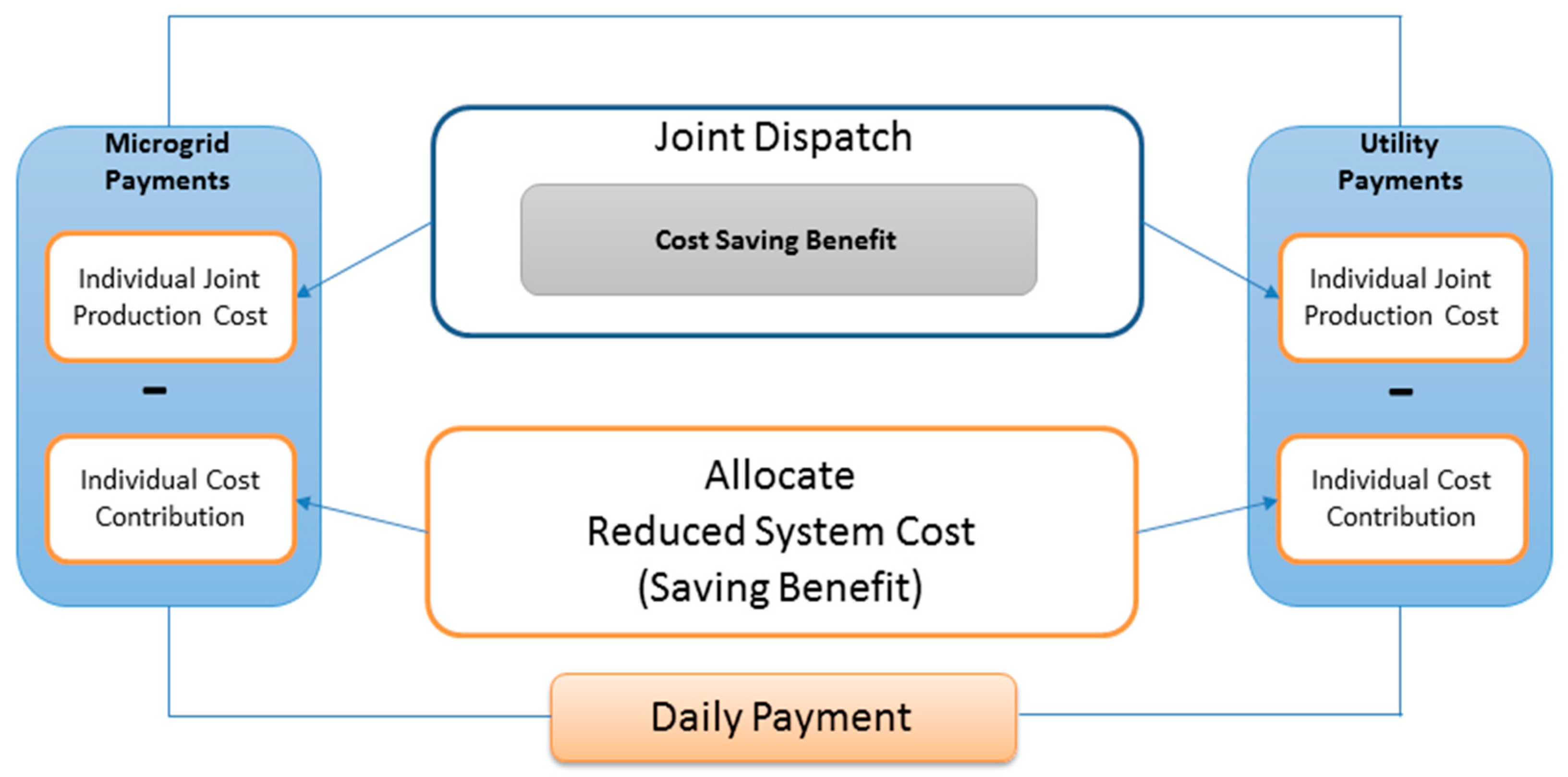
As Shapley values express fair cost contributions of the micro- and utility grids to the coalition of jointly delivering an aggregated load schedule, but does not compensate for energy exchange through mutual payments, this research adopts the Shapley value concept to suggest a payment calculation scheme for energy exchange based on fairly allocating joint generation costs. In this regard, we calculate the fair payments for mutual power transactions as the difference of the Shapley values and the actual generation cost of each grid under joint generation. In other words, applying the Shapley value helps to reconcile for an equitable allocation of operation costs and transaction payments for energy exchange between the systems. Figure 1 illustrates the payment calculation scheme for energy exchange as presented in this research.
The payment calculation scheme determines the cost saving benefit from joint generation and applies the Shapley value to allocate the saving benefit between the micro- and utility grids based on their individual marginal cost contributions to the power exchange coalition. Against the background of different cost contributions, the Shapley value function incentivizes the joint cost optimization and helps to compensate for energy exchange by fairly calculating the payments for the energy exchange between the utility and the microgrid.
2. Shapley Value-Based Decision Model
This research assumes a privately owned microgrid and a hosting utility that operates as interconnected power systems with the objective to minimize individual daily generation costs through energy exchange. Further, we assume that each system has sufficient generation resources to meet its own loads, and can make a decision on whether to operate standalone or in joint generation.
To motivate energy exchange between the microgrid and the utility, we first determine the daily generation costs of standalone operations with no power exchange. We then introduce a coalition model for the two power grids to cooperatively minimize total daily generation costs through energy exchange, where available generation units are centrally committed and dispatched to deliver an aggregated load schedule.
Based on realized cost savings by the coalition in comparison to standalone operations, we adopt the solution concept of Shapley value to determine the respective contributions to cost savings by the microgrid and the utility. The final part of the decisions is who should pay whom by how much in order to fairly compensate for power transactions.
2.1. Notations/Nomenclature
| Index/sets | |
| Distributed generation (DG) units; | |
| Energy storage units; | |
| Utility generating units; | |
| Time periods in 1-hour increments. | |
| Parameters | |
| Microgrid generation cost function; | |
| Constant from generation cost curve for DG unit g; | |
| First order component of generation cost curve for DG unit g; | |
| Second order component of generation cost curve for DG unit g; | |
| Utility generation cost function; | |
| Constant from generation cost curve for aggregated utility unit u; | |
| First order component of generation cost curve for aggregated utility unit u; | |
| Second order component of generation cost curve for aggregated utility unit u. | |
| Power limits | |
| Minimum power level of DG unit g (MW); | |
| Maximum power level of DG unit g (MW); | |
| Minimum power level of the utility (MW); | |
| Maximum power level of the utility (MW). | |
| Energy storage system (ESS) | |
| Charging/discharging efficiency for energy storage system of type s; | |
| Maximum capacity of energy storage system of type s (MWh); | |
| Minimum capacity of energy storage system of type s (MWh); | |
| Maximum amount that can be added (charged) to storage (MW); | |
| Maximum amount that can be drawn (discharged) from storage (MW). | |
| (Given) Forecasts | |
| Sum of power production from renewable energy supply (MW); | |
| Power level demanded from the microgrid loads at time t; | |
| Power level demanded from the utility loads at time t. | |
| Decision and logical variables | |
| Power generated by aggregated utility unit in period t (MW); | |
| Power generated by DG unit g in period t (MW); | |
| Binary indicating if a unit g is on or off in period t; | |
| Energy stored in energy storage system s at the end of period t (MW); | |
| Power output from storage unit s in period t (MW); | |
| Power charged to storage unit s in period t; | |
| Power discharged by storage unit s in period t; | |
| Number of storage unit s in period t. | |
2.2. “As-If” Standalone Generation Cost Models without Energy Exchange
To calculate the individual generation costs from standalone grid operations, the decision model is inserted into the architecture of a single microgrid and a utility grid with fixed system configurations and deterministic input variables that consider their individual load profiles and generation constraints.
Although Bayram et al. [7] suggests additional criteria for the definition of microgrids, e.g., controllable loads, the ability to operate in islanding mode or combined heat and power (CHP), our study only concerns about the electric system of a microgrid with the aim to suggest a proper basis for operational cost sharing with the electric utility.
Given a microgrid with a fixed configuration of distributed generation, a renewable energy source and an energy storage system, the unit commitment (UC) and economic dispatch (ED) for minimum cost generation to meet microgrid loads is formulated as a mixed integer programming [14] problem. To compute the utility’s generation costs under given demands, we treat the utility as an aggregated generation unit, of which the hourly generation cost function is obtained by solving the UC & ED problem of the utility over different load levels, as proposed by Chang et al. [15].
2.2.1. Microgrid Cost Model
Our study describes the deterministic case of an optimization model with determined inputs for the specific dispatch scenario of a summer and a winter day. In this respect, the microgrid produces power from a fixed installed capacity of intermittent renewable energy supply (i.e., solar power) and distributed energy resources (i.e., a gas turbine) to meet the loads demanded by the consumers. For the design of our cost model, renewable energy sources are indicated with zero marginal costs to make sure that renewable generation is fully dispatched.
The aggregated power output from renewables is calculated to the effect of ambient conditions (i.e., solar irradiation) and treated as a negative load for any given load level. Energy storage can help to store excess power and reduce distributed generation in future periods. Excess renewable power is lost in cases where the output from renewable energy exceeds the energy storage capacity.
After determining the power output from renewable energy production, the remaining power output from distributed generation for each load level can be determined. Distributed energy resources generate power whenever renewables and energy storage are insufficient to fully serve the load. The decisions include two parts: whether to commit a distributed energy unit and how much power by a committed unit. The binary UC variables are 0–1 integer variables corresponding to ON-OFF decisions and are continuous ED variables for the generation power levels. Given a microgrid with a fixed configuration, the mixed integer programming problem of UC & ED for system demand satisfaction and generation cost minimization is formulated as follows:
The generation cost of each distributed generation unit is a quadratic function of the generation power level. The UC decisions, , and ED decisions, , must meet various microgrid and unit constraints, and minimize the total generation cost of all the committed distributed generation units over one day as described in Equations (1)–(9).
As the loads must be met at all times in a power system, Equation (2) requires the model to have sufficient generation available to balance demand and supply. Renewable generation is included as negative loads and assumed to be fully dispatched with zero marginal costs.
In addition, there are minimum and maximum power levels for the DG generation units applied to the power output , which are presented in Equation (3).
The implementation of a discrete storage system does not directly affect the objective function but adds storage specific constraints on power flow through charging and discharging of the storage system as represented in Equations (4)–(6). Equation (4) is the energy balance equation of a storage unit s for a time period considering energy conversion efficiencies,
Equation (5) defines the total power output of storage as the difference of total discharging power and total charging power , where we assume constant power in one time period.
Besides Equation (2), the total power supply by the distributed generation and storage units should be more than the difference between the demand and renewable power generation of the microgrid. The total storage output power can be either positive or negative in value. The power balance constraint with inclusion of storage is obtained by modification of that in [16] as follows:
Similar to distributed generation units, storage units are also constraint by power limits (charging rates) and storage limits (battery sizes) as expressed by Equations (7.a) and (7.b).
The limits for the minimum and maximum storage are shown in Equation (8).
Finally, a terminal equality constraint that requires the starting and ending limits of the storage in the battery to be equal is set up in Equation (9).
2.2.2. Utility Cost Model
To obtain the utility cost function that minimizes generation costs, we aggregate all of the available thermal units of the utility network into one equivalent aggregate thermal unit. The ideal definition of an aggregate unit will meet some objective across all levels of output of an aggregate unit [17]. Therefore, we perform unit commitment and economic dispatch over the set of all available thermal units to find the minimized generation cost for each given load level. Next, we derive the aggregated thermal unit by fitting a cost function to the data points of generation cost at each load level. The thermal cost function is approximated by a second order polynomial. The aggregate thermal cost functions for summer (S) and winter days (W) are shown in Table 1.
Relevant cost functions were generated based on different model periods and numbers of thermal generation units. Generation specific information on the thermal generating fleet was provided by Taipower Company. For our studies, we use the cost functions obtained for a scheduling period of 24 h during both summer and winter days. In this regards, we assume that the cost functions for a period of 24 h stays the same every day in a week.
2.3. Joint Generation Cost Model with Energy Exchange
To develop a joint generation cost model for the energy exchange between a microgrid and its hosting utility, it will be assumed that the utility and the microgrid each with their own generation and loads are operating as an interconnected power system where generation is centrally dispatched. In this regard, a centralized market coordinator with complete information regarding the cost functions of all generation units is assumed. Based on this information, its responsibility is to independently dispatch all of the available generation resources and minimize the joint generation cost from delivering an aggregate load schedule.
As mentioned before, in the coalition model between microgrid and utility, there is only one single decision entity and the objective is to minimize daily joint generation costs in an idealistic way by adducing a joint load schedule. The joint generation cost can thus be expressed as a sum of the aggregate cost function of the utility and microgrid generation costs, as presented in Section 2.1 and Section 2.2.
The objective function of the joint generation cost model is presented in Equation (10).
As the loads of both system must be balanced, Equation (2) requires sufficient power generation to fully adduce a joint schedule during all of the time periods. Renewable generation is assumed to be fully dispatched with zero marginal costs and included as deterministic negative loads.
In addition to the power balance constraints, Equations (12.a) and (12.b) include minimum and maximum power levels for the distributed and utility generation units applied to the power outputs and , respectively.
Storage specific constraints are the same as Equations (4)–(9), where the power balance constraint with inclusion of storage is obtained by modification of Equation (6) as follows:
To solve the problem, the decision model is implemented in ILOG CPLEX 12.2 as a mixed-integer quadratic programming (MIQP) problem with second order cost functions to dispatches all available generation resources and minimize the joint generation cost from delivering an aggregate load schedule. CPLEX helps to effectively solve the problem—where the restriction of the problem to its continuous and general integer variables is a convex quadratic program (QP)—as a commercial MIQP solver instead of using standard algorithms.
2.4. Shapley Value Based Decision Model and Payment
To calculate the payments of power exchanged, a method that fairly accounts for individual cost and generation contributions to the joint operation is needed. The Shapley value constitutes as such a method and helps us to compensate for energy exchange through fair payments for power .transactions between the power systems due to a mutually agreeable division of joint operation costs.
The idea is that given a cost sharing game, players join the game one at a time in some predetermined order. As each player joins, a player’s cost contribution is its net addition to the cost as it joins. The Shapley value of a player is its average cost contribution over all possible orderings of the players and supports a mutually agreeable division of costs with certain fairness properties [18].
Mathematically, the Shapley value of player i can be expressed as
where S is the number of players in the coalition, N is the total number of players in the game, is the characteristic function representing the total jointly earned payoff or benefit of a coalition S, and i is any player in the game. The term, v(S ∪ {i}) − v(S), refers to the marginal contribution of player i to the value of the whole coalition v(S). Further, the expression depicts the weighting factor that allocates a proportional share of marginal contribution of each player in the coalition.
As a result, the Shapley value is assigned to a player i according to a given function v that determines the gain v(S) for a coalition game (N, v) with transferable utility for player set N measured by a function v for any non-empty subset S ⊆ N. The advantages of this method are that this approach is budget-balanced and guarantees equilibrium existence in any game regardless of its parameters. Also, it has some important properties that hold when allocating the cost in a cost sharing game [18]:
- Pareto-efficiency: The total value of a coalition is distributed among the members: .
- Symmetry: The value can be determined regardless of the name of the players. If for any two players i and j the following holds: for every subset S ⊆ N with , then .
- Additivity: This property requires for any two games , that: .
- Zero player: If the marginal value of a player to any possible coalition is zero, this player gains a value of zero: .
3. Case Study Results
We design a fictitious interconnection model between the Mueller microgrid in Austin, Texas, and the utility grid in Taiwan for case study to share the savings from their coalition through fair payments for energy exchange and validate out model. Our results are presented for the residential load and PV generation data obtained for the Mueller community as of April 2015 from the Pecan Street Database. The weekly load profile for the Taiwan utility was obtained from Chang et al. [15] and considered for a single day period. The load of a winter day is in average 25% lower than the load of a summer because there is no need for air conditioning or heating in the winter.
Our case study shows that when compared to standalone generation, both the micro- and utility grids are better-off when they collaborate in power exchange regardless of their individual contributions to the power exchange coalition.
Fair payments for both a summer and a winter generation scenarios, however, show that joint savings through energy exchange depend on variations in load profiles and ask for different cost reimbursement during summer and winter.
3.1. Generation Scenarios and Cost Savings from Joint Operation
Table 2 summarizes the production scenarios for the Mueller microgrid as obtained from the cost models presented in the previous sections and distinguishes individual generation costs for the micro- and utility grid from standalone {{m},{U}}, coalition {m,U} and coalition with storage {m*,U}. Analyses of Table 2 show that the joint operation of the utility grid and the microgrid with storage, {m*,U}, minimizes the total daily generation cost among all scenarios.
In the coalition with storage {m*,U} case, the microgrid produces 60.62 MWh per day in its maximum capacity at a cost of $1636 during summer. Due to strictly lower generation costs of utility production during lower peak demand levels in winter, the microgrid produces nothing but solely importing its energy needs from the utility.
For the utility, in comparison to the non-storage case {m,U}, we find that production reduces to 202,397 MWh at a cost of $3,977,685 during summer and 159,755 MWh at a cost of $2,918,003 during winter. Herein, storage helps to reduce the costs from varying load levels by charging power to the battery during times of low demand and discharging power from the battery during times of costly peak demand hours.
By calculating the cost saving benefit from joint operation as the difference between the sum of individual and total generation costs, the power exchange coalition {m*,U} generates daily savings of $850 in summer and $494 in winter, respectively. As discussed, a cost model for joint generation, however, only allows for an assessment of the cost savings but gives no hints on how to share them.
3.2. Joint Generation Cost Allocation between the Utility and Microgrid
Given the cost savings from the joint operations, we adopt the Shapley value concept for a fair division of the benefits by evaluating individual shares in costs incurred by forming the coalition. Based on the individual and joint generation costs summarized in Table 2, the Shapley values for the power exchange coalition {m*,U} are computed according to Equation (14). As mentioned before, the Shapley value of a player is calculated as a player’s net addition to the cost of a coalition (marginal cost) over all possible ordering of the players. Results are listed in Table 3.
Herein, the output of each possible grouping of the participants is shown in the left-hand column of the table. The marginal contribution of a single player to a subgroup is calculated as the output of the subgroup minus the output of the same subgroup excluding the individual participant. For instance, the marginal contribution of {m*} to the output of the overall power coalition {m*,U} in summer of −$239 is equal to the difference between the output of the power coalition {m*,U} of $3,979,321 and the output of the utility {U} of $3,979,560.
By calculating the Shapley value of each player as a player’s marginal cost contribution to the cost of a coalition across all of the subgroups, we find that the cost contribution of the microgrid of $186 is lower for the summer than $324 for the winter case. This is mainly due to the fact that during winter the utility facilitates the total power generation for low peak demands and the microgrid imports all of its energy to contribute to reduced system cost. During summer, on the other hand, the penetration from solar power and the ability to dispatch distributed generation to avoid costly utility peak power plants helps the microgrid to lower its cost contribution for high levels of peak demand.
3.3. Fair Payment Calculation for the Energy Exchange between a Microgrid and the Utility
We calculate the fair payments for mutual power transactions as the difference of the Shapley values and the actual generation cost of each grid under joint generation. In other words, applying the Shapley value helps to reconcile for an equitable allocation of operation costs and transaction payments for energy exchange between the systems.
Table 4 compares the actual generation costs from individual production under joint operations with their cost contribution being determined by the Shapley values. We see that during summer days the actual production costs of $1636 of microgrid generation heavily exceeds its cost contribution of $186. Hence, the microgrid needs to be fairly compensated by the utility for its additional generation during summer and receives $1450 per day for its power transactions. During winter the microgrid doesn’t generate and fully depends on the imports from the utility grid with payments of $324 for its energy imports. To incentivize sharing the savings from energy exchange, therefore, we compensate microgrid saving contributions during summer by utility to microgrid payments, and energy exports from the utility to the microgrid during winter by microgrid payments.
4. Conclusions
This study examined the joint operation of a microgrid and its utility network, and suggested a method to fairly compensate for energy exchange through payments for mutual power transaction based on the individual contributions to reduced daily generation costs when micro- and utility grids agree to collaborate as a single entity where generation was centrally dispatched. For this purpose, we have assumed a privately-owned microgrid interconnected with its hosting utility and developed a centralized decision model to optimally minimize shared generation costs.
To address the problem, the decision model was inserted into the overall architecture of a single microgrid and a utility grid with fixed system configurations and deterministic input variables that considered the electrical load profiles, microgrid and utility generation constraints, ambient conditions, and economic generation data. The decision model presented here was implemented in CPLEX as a mixed-integer quadratic programming (MIQP) problem with second order cost functions. ILOG’s CPLEX 12.2 helped to effectively solve the problems instead of using standard algorithms.
To fairly compensate for energy exchange through payments for mutual energy transactions, we first calculated the “as-if” standalone generation costs for both the microgrid and the utility grid based on the minimized cost of their individually owned generation units with no power exchange between the systems. We then compare the cumulative cost from standalone dispatch with the actual cost under pool dispatch to provide a proper basis to fairly allocate joint operation costs. Justified by its favorable properties to support a mutually agreeable division of joint operational costs, finally, the Shapley value was applied to fairly compensate for power exchanged and to calculate the payments for power transactions between a microgrid and its hosting utility.
In a case study on the model interconnection of the Taipower Company and the Mueller microgrid, we showed that system operation costs can be reduced by minimizing daily operation cost through energy exchange and justified that a method to calculate fair payments for mutual power transactions is needed.
The cooperative game theoretic methodology developed in this paper has laid a foundation for future studies to
- (i)
- including both the cost of supplying thermal and electrical loads to include the efficiency gains from combined heat and power systems in microgrids [19],
- (ii)
- (iii)
- assessing different coalition formation algorithms (e.g., bilateral programming or auction mechanisms) for the energy exchange between micro- and utility grids.
Author Contributions
The research reported in this manuscript has been conducted by Robin Pilling, Shi-Chung Chang, and Peter B. Luh at National Taiwan University (NTU) as part of the MOST 106-2221-E-002-129 project. In this respect, Robin Pilling and Shi-Chung Chang analyzed the challenges and benefits from cooperation in decentralized power grids, and designed the decision framework to propose a payment calculation scheme for the joint generation between micro- and utilty grids. Peter B. Luh contributed to the technical analysis of microgrids, its connection to the utility grid and the associated mathematical problem formulation. Robin Pilling solved the decision problem and analyzed the data to conduct the case study.
Conflicts of Interest
The authors declare no conflict of interest.
References
- Hogan, W.W. A Competitive Electricity Market Model; Harvard Electricity Policy Group: Cambridge, MA, USA, 1993. [Google Scholar]
- Li, F.; Qiao, W.; Sun, H.; Wan, H.; Wang, J.; Xia, Y.; Xu, Z.; Zhang, P. Smart transmission grid: Vision and framework. IEEE Trans. Smart Grid 2010, 1, 168–177. [Google Scholar] [CrossRef]
- Higgins, N.; Vyatkin, V.; Nair, N.C.; Schwarz, K. Distributed power system automation with IEC 61850, IEC 61499, and intelligent control. IEEE Trans. Syst. Man Cybern. Part C 2011, 41, 81–92. [Google Scholar] [CrossRef]
- Chowdhury, S.P.; Crossley, P.; Chowdhury, S. Microgrids and Active Distribution Networks; Institution of Engineering and Technology: Stevenage, UK, 2009. [Google Scholar]
- Hatziargyriou, N.; Sano, H.; Iravani, R.; Marnay, C. Microgrids: An overview of ongoing research development and demonstration projects. IEEE Power Energy Mag. 2007, 5, 78–94. [Google Scholar] [CrossRef]
- Chattopadhyay, D. An energy brokerage system with emission trading and allocation of cost savings. IEEE Trans. Power Syst. 1995, 10, 1939–1945. [Google Scholar] [CrossRef]
- Bayram, I.S.; Shakir, M.Z.; Abdallah, M.; Qaraqe, K. A survey on energy trading in smart grid. In Proceedings of the 2014 IEEE Global Conference on Signal and Information Processing (GlobalSIP), Atlanta, GA, USA, 3–5 December 2014. [Google Scholar]
- Asimakopoulou, G.E.; Dimeas, A.L.; Hatziargyriou, N. Leader-follower strategies for energy management of multi-microgrids. IEEE Trans. Smart Grid 2013, 4, 1909–1916. [Google Scholar] [CrossRef]
- Jain, K.; Mahdian, M. Cost sharing. In Algorithmic Game Theory; Cambridge University Press: Cambridge, UK, 2007; pp. 385–410. [Google Scholar]
- Friedman, E.; Moulin, H. Three methods to share joint costs or surplus. J. Econ. Theory 1999, 87, 275–312. [Google Scholar] [CrossRef]
- Shapley, L.S. A Value for n-person Games. In Contributions to the Theory of Games, Volume II, Annals of Mathematical Studies v. 28; Kuhn, H.W., Tucker, A.W., Eds.; Princeton University Press: Princeton, NJ, USA, 1953; pp. 307–317. [Google Scholar]
- Gopalakrishnan, R.; Marden, J.R.; Wierman, A. Characterizing distribution rules for cost sharing games. In Proceedings of the 2011 5th International Conference on Network Games, Control and Optimization (NetGCooP), Paris, France, 12–14 October 2011. [Google Scholar]
- Tan, X.; Lie, T.T. Application of the Shapley Value on transmission cost allocation in the competitive power market environment. IEE Proc. Gener. Trans. Distrib. 2002, 149, 15–20. [Google Scholar] [CrossRef]
- El-Hawary, M.E.; Christensen, G.S. Optimal Economic Operation of Electric Power Systems; Academic Press, Inc.: New York, NY, USA, 1979. [Google Scholar]
- Chang, S.C.; Chen, C.H.; Fong, I.K.; Luh, P.B. Hydroelectric generation scheduling with an effective differential dynamic programming algorithm. IEEE Trans. Power Syst. 1990, 5, 737–743. [Google Scholar] [CrossRef]
- Xiaoping, L.; Ming, D.; Jianghong, H.; Pingping, H.; Yali, P. Dynamic economic dispatch for microgrids including battery energy storage. In Proceedings of the 2nd International Symposium on Power Electronics for Distributed Generation Systems, Hefei, China, 16–18 June 2010. [Google Scholar]
- Hargreaves, J.J.; Benjamin, F.H. Commitment and dispatch with uncertain wind generation by dynamic programming. IEEE Trans. Sustain. Energy 2012, 3, 724–734. [Google Scholar] [CrossRef]
- Bremer, J.; Sonnenschein, M. Estimating Shapley Values for Fair Profit Distribution in Power Planning Smart Grid Coalitions; Springer: Berlin, Germany, 2013. [Google Scholar]
- Bracco, S.; Delfino, F.; Pampararo, F.; Robba, M.; Rossi, M. A mathematical model for the optimal operation of the University of Genoa Smart Polygeneration Microgrid: Evaluation of technical, economic and environmental performance indicators. Energy 2014, 64, 912–922. [Google Scholar] [CrossRef]
- Billinton, R.; Chen, H.; Ghajar, R. Reliability Evaluation of Power Systems; Plenum Press: New York, NY, USA, 1996. [Google Scholar]
- Razali, N.M.M.; Amir, H.H. Microgrid operational decisions based on CFaR with wind power and pool prices uncertainties. In Proceedings of the 2009 44th International Universities Power Engineering Conference (UPEC), Glasgow, UK, 1–4 September 2009; pp. 1–5. [Google Scholar]
Figure 1.
Payment Calculation Scheme for Energy Exchange.


Table 1.
Aggregated Thermal Unit of the Taipower Company (in $).
| Scheduling Horizon (in h) | No. of Plants | Cost Function of the Aggregated Thermal Unit (in $) 1 |
|---|---|---|
| 24 | 3 | |
| 24 | 7 | |
| 24 | 10 (W) | |
| 24 | 10 (S) | |
| 72 | 10 | |
| 168 | 10 (W) | |
| 168 | 10 (S) |
1 USD to TWD = 31 $.
Table 2.
Generation scenarios and costs for model grids.
| Scenarios | Production (MW) | Individual Generation Cost ($/day) | Total Generation Cost ($/day) | ||||
|---|---|---|---|---|---|---|---|
| Summer | Winter | Summer | Winter | Summer | Winter | ||
| Standalone | {m} | 9.44 | 5.91 | 633 | 585 | 3,980,193 | 2,918,511 |
| {U} | 202,450 | 159,750 | 3,979,560 | 2,917,926 | |||
| Standalone | {m *} | 8.40 | 5.21 | 611 | 571 | 3,980,171 | 2,918,497 |
| {U} | 202,450 | 159,750 | 3,979,560 | 2,917,926 | |||
| Coalition {m,U} | {m} | 60.62 | 0.00 | 1636 | 0 | 3,979,337 | 2,918,015 |
| {U} | 202,397 | 159,755 | 3,977,701 | 2,918,015 | |||
| Coalition {m*,U} | {m *} | 60.62 | 0.00 | 1636 | 0 | 3,979,321 | 2,918,003 |
| {U} | 202,397 | 159,755 | 3,977,685 | 2,918,003 | |||
* Indicates with storage.
Table 3.
Shapley values for the microgrid and the utility.
| Subgroup | Summer (in $/day) | Winter (in $/day) | ||||
|---|---|---|---|---|---|---|
| Subgroup Output | m’s Marginal Contribution | U’s Marginal Contribution | Subgroup Output | m’s Marginal Contribution | U’s Marginal Contribution | |
| {m*} | 611 | 611 | - | 571 | 571 | - |
| {U} | 3,979,560 | - | 3,979,560 | 2,917,926 | - | 2,917,926 |
| {m*,U} | 3,979,321 | −239 | 3,978,710 | 2,918,003 | 77 | 2,917,432 |
| Total | 372 | 7,958,270 | 648 | 5,835,358 | ||
| Shapley-Value (Average) | 186 | 3,979,135 | 324 | 2,917,679 | ||
Table 4.
Actual generation cost and daily payments for power exchange.
| Summer (in $/day) | Winter (in $/day) | |||
|---|---|---|---|---|
| m’s Share | U’s Share | m’s Share | U’s Share | |
| Actual Production Costs | 1636 | 3,977,685 | 0 | 2,918,003 |
| Shapley-Value | 186 | 3,979,135 | 324 | 2,917,679 |
| Daily Payment | - | 1450 | 324 | - |
© 2017 by the authors. Licensee MDPI, Basel, Switzerland. This article is an open access article distributed under the terms and conditions of the Creative Commons Attribution (CC BY) license (http://creativecommons.org/licenses/by/4.0/).
Share and Cite
MDPI and ACS Style
Pilling, R.; Chang, S.C.; Luh, P.B. Shapley Value-Based Payment Calculation for Energy Exchange between Micro- and Utility Grids. Games 2017, 8, 45. https://doi.org/10.3390/g8040045
AMA Style
Pilling R, Chang SC, Luh PB. Shapley Value-Based Payment Calculation for Energy Exchange between Micro- and Utility Grids. Games. 2017; 8(4):45. https://doi.org/10.3390/g8040045
Chicago/Turabian StylePilling, Robin, Shi Chung Chang, and Peter B. Luh. 2017. "Shapley Value-Based Payment Calculation for Energy Exchange between Micro- and Utility Grids" Games 8, no. 4: 45. https://doi.org/10.3390/g8040045
Note that from the first issue of 2016, this journal uses article numbers instead of page numbers. See further details here.