
Auctions Versus Private Negotiations in Buyer-Seller Networks

Department of Economics, Southern Illinois University, Carbondale, IL 62901,USA
Games 2016, 7(3), 22; https://doi.org/10.3390/g7030022
Submission received: 7 July 2016
/
Revised: 17 August 2016
/
Accepted: 24 August 2016
/
Published: 31 August 2016
Abstract
:Buyer-seller networks where price is determined by an ascending-bid auction are important in many economic examples such as certain real estate markets, radio spectrum sharing, and buyer-supplier networks. However, it may be that some sellers are better off not participating in the auction. We consider what happens if sellers can make a take it or leave it offer to one of their linked buyers before the auction takes place and thus such a seller can choose not to participate in the auction. We give conditions on the graph and buyers valuations under which the buyer and seller will both agree to such a take it or leave it offer. Specifically, the buyer-seller pair will choose private negotiation over the auction if the seller acts as a network bridge with power over the buyer and if there are enough buyers with low valuations so that the seller does not expect to receive a high price in the auction.
JEL:
C7; D44; D851. Introduction
Auctions are often better for sellers than private negotiations or posted pricing when buyers have independent private values; see Bulow and Klemperer [1], Wang [2], and Zhang [3]. However, such negotiations and auctions generally take place in a non-network environment. We consider a network of buyers and sellers where the price is determined by an ascending bid auction and ask when a seller in such a network would prefer not to participate in the auction, but instead to privately negotiate with one of his linked buyers. In a networked environment, if similar items are for sale in adjoining neighborhoods, the seller may not expect to obtain a high price in the auction and may prefer private negotiations especially if that seller has some degree of network power over certain buyers.
Specifically, we consider buyer-seller networks with an ascending bid auction; such an auction is a simple way to ensure that the availability of similar items in adjoining neighborhoods will influence the auction price. Before the auction occurs a randomly chosen seller can make a take it or leave it offer to one of his linked buyers. The buyer can accept this price or the buyer can choose to return to the auction that will take place without the seller; once the seller chooses to make an offer he can commit to no longer participating in the auction perhaps because advance notification of a seller’s participation is required. We give conditions under which the buyer and seller will both agree to such a take it or leave it offer and thus will choose to opt out of the auction. Specifically, the seller is able to make such an offer if (i) he acts as a bridge in the network where if he is removed then the initial graph splits1 and if (ii) buyers’ valuations are spread out so that the probability of a buyer having a low valuation is large enough that the seller’s expected price from participating in the auction is low and/or the probability of a buyer having a high valuation is large enough so that a buyer is willing to accept the seller’s offer. The results are extended to the case of a seller making multiple offers to linked buyers and it is shown that this increases the range of prices where opting out occurs. Results are given for both the case of an allocatively complete initial graph and the case of an allocatively incomplete initial graph and conditions are given under which opting out is more likely to occur in the second case.
There are many examples where buyer-seller networks use auctions to determine prices or alternatively where an ascending bid auction can be used to represent the price. One well known example is real estate auctions. Many countries such as Australia, New Zealand, Ireland, and Scotland use auctions to determine prices in real estate markets where sellers can choose to either auction off a property or to negotiate a private deal2; see Maher [9], Lusht [7], and Thanos and White [10]. Additionally, in the U.S. there are websites (such as hubzu.com) for non-foreclosure real estate sales which use auctions as the price mechanism. Real estate sales can be interpreted as taking place on a network since the seller’s property has a particular location and each buyer also has a certain location (or locations) where he wishes to purchase property; these locations create buyer-seller links. However, it may be the case that a seller would prefer to make an offer to a particular buyer directly rather than go through the auction.
Another example is that of secondary spectrum sales where a primary spectrum user (such as a cell phone provider or a TV broadcaster) holds a license to use a specific radio spectrum band in a given area. Unlicensed secondary users would like to access the spectrum by purchasing idle spectrum channels from primary users whose license covers their location. These locations create a buyer-seller network where a link indicates a secondary user (or buyer) is located in a primary user’s (or seller’s) licensed area; see Zhang and Zhou [11]. The electrical engineering literature often suggests auctions as the best mechanism for such sales3; see Zhang, et al. [12] and Chun and La [13]. However, it may be that the primary license holder would prefer to opt out of the auction and make an offer directly to a certain buyer.
The model also incorporates other buyer-seller networks where a formal auction does not take place, but where an ascending bid auction may be used to approximate prices. Blume et al. [14] shows that the prices resulting from an ascending bid auction in a buyer-seller network can be achieved using a game of bid and ask prices instead of using an actual auction; thus one can interpret the auction as being a simple way to calculate prices with desirable efficiency properties in buyer-seller networks. Additionally, Bulow and Klemperer [1] note that an ascending bid auction price is the lowest competitive market clearing price; see also Shapley and Shubik [15]. Examples of buyer-seller networks without a formal auction mechanism include a network of clothing assemblers and garment manufacturers, as well as other buyer-supplier networks such as those in the Japanese electronics industry and the Turkish automobile industry; see Lazerson [16], Nishiguchi and Anderson [17], and Wasti et al. [18]. Finally, Niederle and Roth [19] examine the gastroenterology labor market and show that pre-existing or network ties can affect the early exit from the market.
Kranton and Minehart [20] also examine buyer-seller networks where goods are sold in an ascending bid auction. They show that for a given link pattern the equilibrium prices are pairwise stable in that no linked buyer and seller can renegotiate and obtain a better deal. Corominas-Bosch [21] also consider buyer-seller networks where prices are posted and determined through collective bargaining. Note that in our model players opt out before the auction takes place which is different from the renegotiation that takes place ex-post in Kranton and Minehart [20]. Another difference is that in our game after the seller makes the take it or leave it offer he cannot return to the auction. To show that the offer is credible the seller exits the auction (or simply never enters the auction) and after he makes his offer the auction proceeds without him.
The seller prefers not to return to the auction even if his take it or leave it offer is rejected as doing so increases his bargaining power. In Section 3.3, a seller who makes an offer can also choose to either commit to not joining the auction if his offer is rejected or can choose to not make this commitment. Conditions are given under which the seller is better off if he chooses to commit to not joining the auction as his price offer can then be larger. Alternative reasons for not joining the auction can be given as follows. For instance, it could be that the auction requires some advance notification as in a real estate auction where a seller’s participation must be announced four to six weeks in advance. Alternatively, consider a market with repeated sales4 such as radio spectrum sharing or a network of clothing assemblers and garment manufacturers. Here the seller may credibly choose not to return to the auction to gain believability as a tough negotiator in the future. If he does not return to the auction, then if the game is repeated the buyers will know he will not return to the auction and will be more willing to accept his current offer.
There is a large literature on buyer-seller networks. Some papers focus on cooperative approaches to buyer-seller bargaining such as seller cooperatives or Nash bargaining; see Wang and Watts [23] and Bayati et al. [24], respectively. While others consider de-centralized bargaining with bilateral opportunities; see Abreu and Manea [25], de Fontenay and Gans [26], Condorelli and Galeotti [27], and Hatfield et al. [28]. Alternatively, Elliott [29] allows buyers and sellers to invest in relationships and shows that over-investment results when players wish to create outside options while Board and Pycia [30] considers buyer-seller networks where the buyer has an outside option. We add to this literature by focusing on what happens if sellers can choose to exit the market.
The current paper is also related to exchange networks in the sociology literature. There are many papers looking at the relationship between network position and power in exchange networks; see Markovsky, Willer, and Patton [31], Cook and Yamagishi [32], Lucas et al. [33], and Skvoretz and Willer [34]. Here one agent may have power over another if he controls the others resources. In the economics literature, Manea [35] considers a player’s strength in infinite horizon buyer-seller networks with random matching. In the current paper, we find that a seller who acts as a bridge has power over some buyers and may be able to entice such buyers to opt out of the auction.
The paper proceeds as follows. The model and results are presented in Section 2 and Section 3 and extensions to the basic model are found in Section 3.1 and Section 3.2. Concluding remarks are provided in Section 4.
2. Model
Let represent the set of sellers and the set of buyers in a region. Assume . Without loss of generality, assume that each seller has one unit of the good to sell.
Buyer j can purchase from seller i only if i and j are linked. We let g represent the set of links between sellers and buyers and G represents the set of all possible such graphs. We use notation to represent a link between i and j. We let represent the graph that would be obtained when i and all of i’s links are removed from graph g. Let . Let . A path in g connecting i to j is a set of links such that each link is in g. We define to be a component of g if for every and there exists a path in c connecting i to j, and for every and (or for every and ) implies . We let represent the cardinality of and represent the cardinality of .
Let i pay a cost for maintaining each of his links and let j pay a cost for maintaining each of his links .
Buyer j would like to purchase at most one unit of the good where represents the value that j would receive from using the unit. Specifically, it is assumed that each is a random variable independently and identically distributed on with continuous distribution F, where . We let represent the ℓth highest order statistic of a given set of η values and let represent its density function. Additionally, let if and if .
Next we describe the game which determines prices. First, a seller is picked at random. This seller can choose to participate in the auction described below or can choose to make an offer of to any buyer j such that . Buyer j can either agree to pay price for the good, or can refuse to pay the price and can choose to participate in the auction that takes place without seller i. Buyer j must be linked to another seller besides i in order to participate in the auction that takes place without i. Once seller i has decided to negotiate with j instead of participating in the auction, then this decision is final. By exiting the auction the seller gains bargaining power and we assume the seller can commit to not returning perhaps because advance notice of auction participation is required of sellers. We assume all other sellers participate in the auction.
Next the auction takes place either over g or over depending on whether or not seller i chooses to opt out of the auction. In either case, the sellers participating in the auction simultaneously hold ascending-bid auctions as in Kranton and Minehart [20]. Similar to a Walrasian auction the going price is the same across all sellers; we assume the initial price starts at . As the price increases each buyer can decide to drop out of the auction with each of his linked sellers or not. The price rises until enough buyers have dropped out so that demand equals supply for a subset of sellers; these sellers sell at the current price. If there are remaining sellers the price continues to rise until all sellers have sold their goods. The price that seller i receives in the auction is represented by .
Seller i receives utility where
Buyer j receives payoff where
Next we define an allocatively complete network. This definition is from Kranton and Minehart [20]. Network g is allocatively complete if and only if for every of size m, there exists a feasible allocation such that every obtains a good.
Remark 1.
The auction in the current paper is an ascending bid simultaneous auction. We make this assumption because when g is allocatively complete such an assumption guarantees efficient sales in that the buyers with the top m values are the ones who obtain the goods; see Kranton and Minehart [20]. If instead we allow the goods to be auctioned off sequentially in separate ascending bid auctions the goods may end up being assigned inefficiently. To see this consider the following example. Let m=3, n=4, and g=11, 13, 23, 22, 32, 34. Let for all j. Then in a simultaneous ascending bid auction buyers 1, 2, and 3 all obtain the good at price . Next consider a sequential auction where seller 2’s item is auctioned off first; this item will be sold to buyer 2 at price . Next let seller 3’s item be auctioned off. Seller 3 is linked to two buyers 2 and 4, but buyer 2 has already purchased the good. Thus seller 3 will end up selling the good to buyer 4 at a price of . This sale is inefficient in that buyer 4 who values the good the least ends up purchasing the good. In order to avoid this situation we model the auction as taking place simultaneously.
3. Results
We start with the proposition which shows that a seller may gain from not participating in the auction, but from instead just offering a price to a particular buyer that he is linked to for the good.
Assumption A1.
Let g be allocatively complete and consist of a single component and let consist of at least two components for some . Choose a such that and such that j is not guaranteed a good in the auction over even if . Let be the component of that j is a member of and let c be allocatively complete.
Under Assumption A1 seller i acts as a bridge in graph g in that his removal splits the graph into two or more components. When this split occurs buyer j is no longer guaranteed a good even if he has one of the top values. (There are goods for sale in the auction over .) Proposition 1 gives conditions under which seller i can use his position as a bridge to entice buyer j to opt out of the auction.
Remark 2.
Next we show that such a j exists that meets Assumption A1. Note that it is not possible for a component of to consist of only sellers and not buyers as g was a single component and simply removes one seller from g and by definition sellers are not connected to each other; thus, all components of consist of either only buyers or of both buyers and sellers. As consists of at least two components, there must be at least one component that has less than sellers; call this component c. As c has less than sellers it is not possible for buyers to purchase from c. Thus, there must exist a such that and such that j is not guaranteed a good even if .
For simplicity, in the remainder of the paper we set the costs of maintaining links for all i and j with the understanding that adding in such costs will only strengthen our results in the sense that it will increase the cost of staying in the auction and thus will make opting out more likely for both agents.
Proposition 1.
Let Assumption A1 be true for some and . Seller i and buyer j will choose to opt out of the auction and exchange the good at price if for , and if for , .
Note that the condition guarantees that seller i expects to be better off exchanging the good at price given F while guarantees that buyer j expects to be better off participating in the exchange given .
Proposition 1 shows that the seller and buyer will prefer to opt out of the auction if the seller acts as a bridge in the network with some power over the buyer. And if the buyer’s valuations are spread out so that there are enough high value buyers to make the seller think his offer may be accepted and/or enough low value buyers so that the price the seller expects to receive in the auction over g is not too high.
Proof.
Consider the case where ; we show that buyer j will choose to opt out of the auction if the conditions of Proposition 1 are met. If j decides to opt out of the auction, then he will receive a payoff of . If j decides to participate in the auction over graph , then by assumption c is allocatively complete and so the items in component c will sell to the buyers in c with the top values at price . Thus j will win an item only if . So j’s expected payoff from participation in the auction is . So j prefers to opt out of the auction if or if .
Now we show that seller i will choose to opt out of the auction if our conditions are met for the case where . Seller i will prefer to opt out if his expected payoff from opting out is greater than his expected payoff from participating in the auction over g. If i participates in the auction, then he expects for the good to be sold at the price . Since g is allocatively complete, the buyers with the top m values for the good will all win an item and the items will be sold at price ; thus, i expects to receive from participating in the auction. If seller i decides to opt out of the auction, then his expected payoff is accepts ). Since , we know that j accepts if . Thus, i’s expected payoff from opting out is . So if , then i will choose to opt out of the auction.
Next we consider the case where . If , then there are no sellers in the component that j is a member of in network . Thus, if i makes an offer of to j, then if j rejects the offer j will not receive a good and will end up with a payoff of 0. Thus j only rejects the offer if and i will only make the offer if his expected payoff from the offer, , is greater than his expected payoff from participating in the auction over g, . ☐
Remark 3.
Next we discuss how Proposition 1 would be affected if sellers could post reserve prices. If seller i can post a reserve price, then he will expect a higher payoff from participating in the auction over g. Note that i can always post a reserve price of which will guarantee him the same payoff as in the auction with no reserve price; thus, he will only post a reserve price greater than if he expects a higher payoff from doing so. As i’s payoff from the auction increases i will need a larger price to opt out of the auction and the left hand side of the inequalities given in Proposition 1 will increase. Alternatively, if buyer j faces a reserve price, then the probability that he wins the auction over will decrease and the expected price that he pays from winning this auction will increase. Thus, buyer j’s expected payoff from participating in the auction over will decrease. So j will be willing to accept a lower price to opt out of the auction and the right hand side of the inequalities given in Proposition 1 will increase. Thus, adding a reserve price will change Proposition 1 quantitatively but not qualitatively. Notice too that there are different types of reserve prices that could be implemented. For instance, there could be link-specific reserve prices, seller-specific reserve prices, or uniform reserve prices. The choice of such a reserve price will also quantitatively affect Proposition 1. For instance, a seller-specific reserve price or a link-specific reserve price will not affect all buyers and sellers; thus, only some buyers and sellers will see all or part of the price range for increase. For example, if i uses a seller-specific reserve price then only the auction over g will be affected not the auction over . Thus, the left hand side of the inequalities given in Proposition 1 will increase but the right hand side will not change.
Proposition 1 gives a range of which is acceptable to i given F and acceptable to j given for opting out of the auction. This range depends on the probability of exceeding . So, we can find the price which is best for the seller, but we must take this dependence of on into account; this is done in the following corollary.
Let if and if .
Let if and if .
Corollary 1.
If , then seller i will offer to buyer j.
By Proposition 1, buyer j will accept if when and if if .
Next we illustrate Proposition 1 with an example.
Example 1.
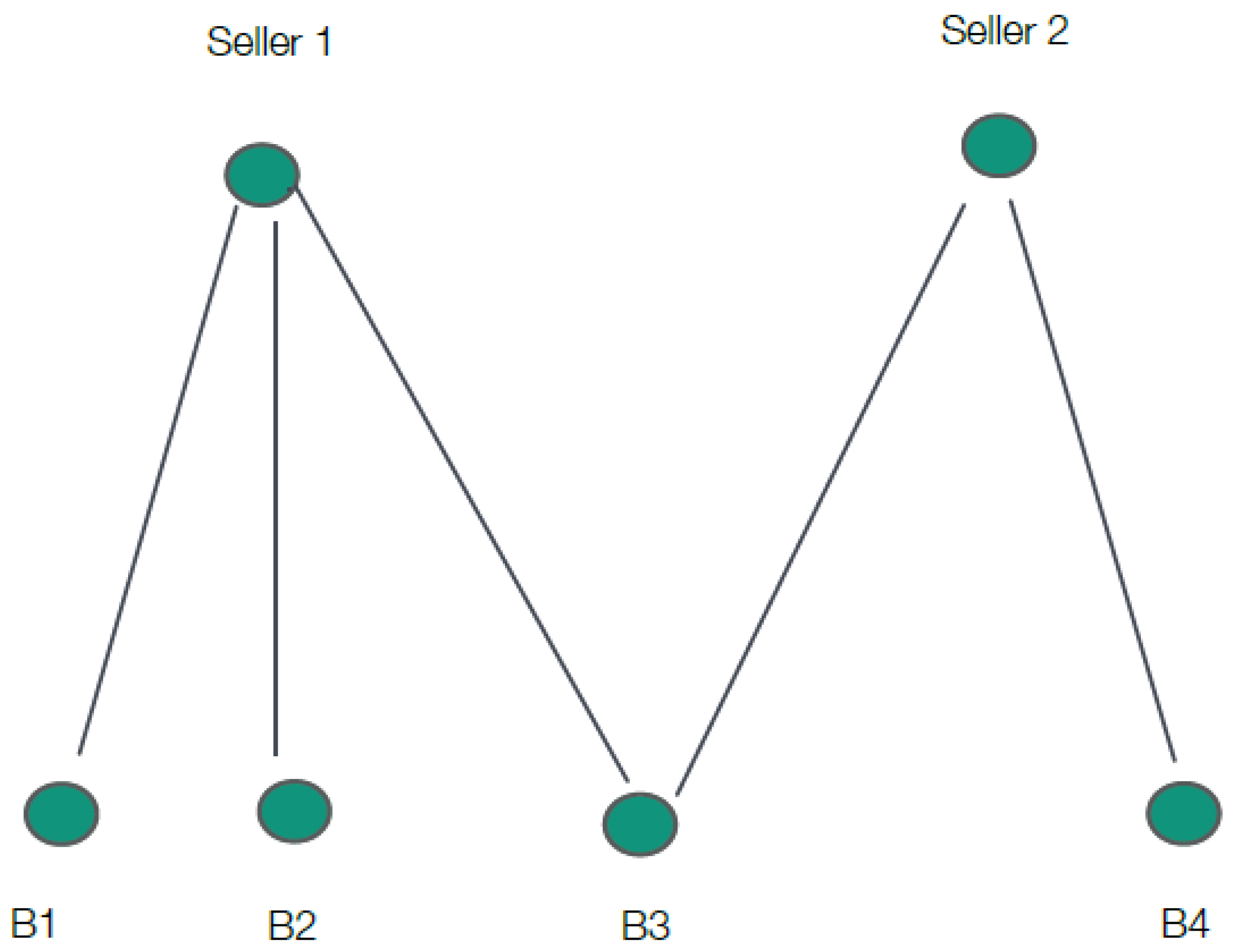
Let , , and which is represented in Figure 1. Let each with equal probability. In an ascending bid auction over g the buyers with the top three valuations each win a good at price where ; note that () is the probability that at least one of the ’s equals 1 or the probability that = 1. Next we consider the graph without seller 2 and all of his ties which we call . Seller 2 can offer price to buyer 2. Buyer 2 will accept this price if doing so makes him better off than he is from participating in the auction over . If , then buyer 2 expects to pay price in the auction over . To see this note that the component of that buyer 2 is a member of is . Thus, buyer 2 wins the item if buyer 1 has and expects to pay price . While if , then buyer 2 expects to win the item with probability and pay price . Thus, buyer 2 expects to win the item with probability Here buyer 2’s expected payoff from entering the auction is: If , then buyer 2’s expected payoff from the auction is . If , then . If buyer , then . Therefore, if and if buyer 2 has valuation or , then if 2 opts out of the auction he will receive a payoff of if and a payoff of if . Thus both types of high value buyers will choose to accept . Seller 2 will receive a payoff greater than his payoff from the auction over g if 2 . Given that , buyer 2 will accept if he has one of the top two valuations and this occurs with probability . Thus if , then seller 2 prefers to opt out of the auction. So for any , both seller 2 and the top value buyers are better off trading the good at price . Note that since the probability of buyer 2 accepting is equal to for all , seller 2’s expected payoff will be maximized at the largest price in this range. Seller 2 cannot gain from raising the price and only selling to a buyer with as the most this buyer would pay is , but the probability of acceptance (or of the buyer being this type) would fall to ; thus, seller 2’s expected payoff from such an offer would be lower than if he set .
Remark 4.
It is assumed that if a seller makes a price offer to one of his linked buyers, then he can commit to not participating in the auction if the offer is rejected perhaps because of institutional rules that govern auction participation. Next, we discuss the credibility of such non-participation in the absence of institutional rules. In Section 3.3, the game is altered so that the seller can choose participation or non-participation in the auction if the price offer is rejected. Proposition 4 gives conditions under which the seller prefers non-participation to participation; the seller prefers such non-participation because it allows him to make a higher price offer to the buyer. Thus, at the beginning of the game the seller would be willing to sign an enforceable contract with the buyer stating that he will pay the buyer a sum of $x if he participates in the auction after his offer is rejected (or alternatively the seller could have a neutral third party hold the $x until the end of the game). By choosing a large x it will never be worth it for the seller to renege on the contract and the buyer can be assured that the seller will not enter the auction after a failed negotiation. Signing such a contract would be a way that the seller could ensure the credibility of non-participation in the absence of institutional rules that assure non-participation.
3.1. Price Offers to Multiple Buyers
Next we allow a seller to make price offers to multiple buyers that he is tied to. Specifically, seller i can simultaneously offer price to all buyers j such that . Each buyer j can either agree to pay price for the good or can refuse to pay the price and then can participate in the auction that takes place without seller i. If multiple buyers agree to pay price , then seller i picks one at random to sell the good to and the remaining buyers can then participate in the auction that takes place without seller i5.
Example 2.
This is a continuation of Example 6 where now seller 2 can make simultaneous offers of to both buyers 2 and 3. Note that if buyer 2 has one of the top two values, then he will agree to opt out of the auction as long as since any price lower than will guarantee that he receives a payoff greater than what he would get if he remains in the auction without seller 2. Similarly, if buyer 3 has one of the top two values he will agree to opt out if . We know from Example 6, that seller 2 will agree to opt out of the auction if 2 3 . Buyer 2 or 3 will accept if he has one of the top two values. Thus, the probability that buyer 2 or 3 accepts is equal to the probability that one or both of these buyers has or . This probability equals . Thus seller 2 opts out if or if . So now for any , both seller 2 and the top two buyers are better off opting out of the auction. Notice that allowing the seller to make more offers has increased the range of prices which support opting out of the auction as the range in Example 1 is smaller at .
Next we generalize this example in the proposition below.
Proposition 2.
Let Assumption A1 be true for seller i and for all . Seller i and buyers will choose to opt out of the auction and exchange the good at price p if and if p satisfies all of the right hand side inequality constraints listed in Proposition 1.
Comparing Propositions 1 and Remark 4 we see that the range of prices that allow for opting out has increased. Thus, as the seller can make more offers the probability that his offer is accepted increases and he does not need to charge as high of a price to opt out. Note that even though all buyers choose to opt out only one of them will end up with the good and the others will rejoin the auction.
Proof.
We show that if p satisfies the inequalities given in Proposition 2, then i and will all choose to opt out of the auction. Since the right hand side inequality constraints from Proposition 1 are met, we know from the proof of Proposition 1 that all will prefer to opt out of the auction. Next we show that seller i will also prefer to opt out. Seller i prefers to opt out if his expected payoff from opting out is greater than his expected payoff from participating in the auction over g. Recall that the good is sold at price in the auction over g. Thus, i prefers to opt out if at least one of accepts . Since the Assumptions A1 are met for all we know that any will accept the offer p if . Thus, the probability that at least one of accepts p equals and so i will choose to opt out if .
Corollary 2.
If the conditions of Proposition 1 are met so that each i and pair choose to opt out of the auction, then the conditions of Proposition 2 will also be met and i and will also choose to opt out of the auction collectively.
Proof.
First we show that if i and meet the conditions of Proposition 1 sufficient for each i and pair to opt out of the auction, then there exists a p that meets all of the inequalities of Proposition 1. To see this note that the left hand side inequalities are for . As we have assumed that each is identically distributed we know that is the same for all . Thus is the same for all j. So choosing a will meet all of the inequalities of Proposition 1.
Next we show that the conditions of Proposition 2 are met. As it must be that and Proposition 2 holds true. ☐
3.2. An Allocatively Incomplete Initial Graph
Next we consider the case where the graph g is not allocatively complete; thus, it is possible for a buyer without a top m valuation to receive the good in an ascending bid auction. We assume here that there is at least one seller who acts as a bridge and who does not contribute to this inefficiency, and show that such a seller has even more to gain from exiting the auction.
Next we define an allocatively complete seller. Let be the set of buyers who are linked to seller in g. Then i is an allocatively complete seller if for all of size m such that there exists a feasible allocation such that every obtains a good.
Assumption A2.
Let g not be allocatively complete and let g consist of a single component. Let there exist such that i is an allocatively complete seller in g and such that consists of at least two components. Choose a such that and such that j is not guaranteed a good in the auction over even if . Let be the component of that j is a member of and let c be allocatively complete.
Under Assumption A2, seller i acts as a bridge and i is an allocatively complete seller. Thus, i’s removal splits the graph, but i does not contribute to the allocative incompleteness of graph g in the sense that buyers linked to i are always guaranteed a good if they have a top valuation.
Proposition 3.
Let Assumption A2 be true for some and . Seller i and buyer j will choose to opt out of the auction and exchange the good at price if for , and if for , . For some .
Proof.
The assumptions of Proposition 3 differ from those of Proposition 1 in that g is no longer allocatively complete, but i is an allocatively complete seller. Note that there have been no changes to the assumptions on buyer j. Thus by Proposition 1, buyer j will choose to opt out of the auction and exchange the good at price if for , and if for , .
Next we show that seller i will also choose to opt out of the auction. First we show that i’s expected payoff from participating in the auction is . Since i is an allocatively complete seller we know that if the top m value buyers include at least one buyer in , then all top value buyers will obtain the good at price . However, as g is not allocatively complete there exists a subset of buyers of size m such that not all of them can obtain the good; additionally, as it must be that . Let this subset of buyers have the top m values. As i is an allocatively complete seller it must be that none of these buyers are linked to i. Thus, i will not sell his good to one of these top value buyers. Instead i will sell his good to a buyer with value or lower and thus he must sell the good to this buyer at a price . Thus, i will either sell the good at or at a lower price and so the expected price that i receives from participating in the auction is . If i decides to opt out of the auction, his expected payoff is accepts ). As in Remark 1, j accepts if . Thus, i’s expected payoff from opting out is . Therefore, i opts out of the auction if or if where . ☐
Next we give an example which illustrates Proposition 3.
Example 3.
Let , and . This graph is illustrated in Figure 2 where represents buyer j. Let and let each occur with equal probability. First notice that seller 2 is an allocatively complete seller since if buyers 3 or 4 have at least one of the top two valuations, then all the top value buyers can receive the good. However, if buyers 1 or 2 have the top two valuations, then they cannot both receive the good; thus g is not allocatively complete. Next we consider the sellers expected payoffs if both sellers participate in an ascending bid auction. Notice that if or if , then . In all other cases . While if either and or if and . In all other cases . Thus, and . Since seller 2 expects to receive half of the time this seller may benefit from exiting the auction and selling directly to buyer 4 who is not linked to any other seller and so cannot remain in the auction if seller 2 opts out. If seller 2 offers to sell directly to buyer 4 at price , then his expected payoff is . If seller 2 participates in the auction, he expects to receive 6. If instead seller 2 sells directly to buyer 4 at price , then he expects this price to be accepted half of the time and he expects to receive . Buyer 4 is not linked to any other seller except seller 2; thus by Proposition 3 he accepts as long as . In the language of Proposition 3, if , then both seller 2 and any buyer 4 with will choose to opt out of the auction. Note that .
Comparing Proposition 1 to Proposition 3 we find that an allocatively complete seller in an allocatively incomplete graph is more likely to opt out of the auction than a seller in an allocatively complete graph; the price range of acceptable offers is larger in Proposition 3 since the left hand side of the price range is lower and the right hand side is the same. In Proposition 3, seller i does not contribute to the allocative incompleteness of the graph and so i may not receive as high of a price in the auction over g as he would if g were allocatively complete. Intuitively, i has no power over particular buyers in g, but as g is allocatively incomplete another seller may. Thus, i is at a disadvantage and may receive a lower price in the auction over g; this makes i willing to accept a lower price from j to opt out of the auction. In Example 3, seller 2 is allocatively complete and seller 1 is not. Here seller 1 can receive a price higher than in the auction over g while seller 2 can receive a price lower than . If g were allocatively complete, then all sellers would receive price in an auction over g. Thus, seller 2 expects to do worse than in the allocatively complete case and so he is willing to accept a lower price to opt out.
3.3. Increasing the Seller’s Options
Next we examine what happens when the seller can choose to remain in the auction even if he makes a price offer to a buyer. Thus, the game is altered so that after a seller is picked at random this seller can choose to either: (1) participate in the auction over g; (2) make an offer of to any buyer j such that and commit to not joining the auction if the offer is rejected; or (3) make an offer of to any buyer j such that and join the auction over g if the offer is rejected. Note that if the seller picks option 2 and the offer is rejected, then the auction will take place over as before. Proposition 4 gives conditions under which the seller prefers the second option of making an offer and opting out of the auction.
Before presenting the proposition we first extend Example 1 to allow for the additional seller’s choice. In this example, the seller prefers to commit to not joining the auction if the offer is rejected as this decision allows him to make a higher offer to the buyer.
Example 4.
Recall from Example 1 that , , , and each with equal probability. First, we consider the auction over g. From Example 1, seller 2 expects to sell his item at price . Next, we determine the payoff that buyer 2 expects to receive from the auction over g. If , then buyer 2 expects to receive a payoff of . Here is the probability that buyer 2 wins an item as buyer 2 always wins the item unless all other buyers also have a valuation of 10 in which case three of the four buyers are selected at random to win an item. And is the probability that buyer 2 wins the item and pays a price of 1 which occurs if at least one of the other buyers has a valuation of 1. If , then buyer 2 expects to receive payoff . And if , then . If seller 2 chooses to make offer and to remain in the auction over g if is rejected, then seller 2 must expect a payoff at least as high as he would get from just participating in the auction over g; so . Buyer 2 will accept this offer when if or . If , then buyer 2 accepts if . And if , then buyer 2 accepts if . Seller 2 maximizes his expected profits by setting in which case buyer 2 accepts this offer half of the time and otherwise rejects the offer in which case seller 2 participates in the auction; seller 2’s expected profits equal . If instead seller 2 chooses to make an offer of and commit to not returning to the auction, then we know from Example 6 that he chooses a price such that and that this offer will be accepted half of the time. To maximize profits here seller 2 sets and receives expected profits equal to . Thus, seller 2’s expected profits are higher if he commits to opting out of the auction when he makes an offer.
Next we generalize the results of the example in Proposition 4.
Define .
Proposition 4.
Let Corollary 1 hold true for some i and j. Then seller i prefers to make a offer to j and to opt out of the auction than to make offer to j and to remain in the auction, if .
Proof.
First, consider the case where seller i offers to j and opts out of the auction. From Corollary 1 and the discussion preceding this corollary, seller i’s expected payoff is maximized when and equals . Next, consider the case where seller i offers to buyer j and remains in the auction. Here i expects to receive a payoff of since if i’s offer is rejected then i enters the auction and expects to receive . Buyer j will accept offer if his payoff from accepting is greater than his expected payoff from entering the auction over g or if or if . Thus, if i wants to maximize his expected payoff he will offer price .
Seller i is better off opting out of the auction and offering than opting in and offering if . Note that seller i only offers and opts out if doing so is better than participating in the auction or if . Thus, if , then . ☐
4. Concluding Remarks
We have given conditions under which it is optimal for a seller not to participate in an auction over a buyer-seller network. Specifically, a seller will choose to opt out of the auction if the seller acts as a bridge in the network and if there is a considerable likelihood of low value and/or a considerable likelihood of high value buyers. A considerable likelihood of low value buyers decreases the expected price the seller expects to receive in the auction making him more likely to exit. While a considerable likelihood of high value buyers makes it more likely that the buyer who receives the opting out offer will be willing to take it. We also extend the results to the case where a seller can make offers to multiple buyers and show that this makes opting out more likely. Additionally, we extend the results to the case where the initial graph is not allocatively complete.
The model could naturally be extended to a repeated game framework, which we leave for future research. Such an extension is important in many examples such as spectrum sharing networks and networks of clothing assemblers and garment manufacturers. In both of these examples, goods are sold on a network repeatedly. It would be interesting to investigate how such repetition influences whether or not a seller chooses to opt out of the network. For instance, in a repeated game it may be possible for a seller to learn the valuation that a linked buyer has for the good. Such knowledge could increase the likelihood that a seller will choose to opt out of a network with a particular buyer.
Acknowledgments
Financial support from the NSF under grant SES-1343380 is gratefully acknowledged. I also thank two anonymous referees for valuable comments.
Conflicts of Interest
The author declares no conflict of interest.
References
- Bulow, J.; Klemperer, P. Auctions versus negotiation. Am. Econ. Rev. 1996, 86, 180–194. [Google Scholar]
- Wang, R. Auctions versus posted-price selling. Am. Econ. Rev. 1993, 46, 345–356. [Google Scholar]
- Zhang, H. The Optimal Sequence of Prices and Auctions. 2015. Available online: http://ssrn.com/abstract=2401469 (accessed on 6 March 2015).
- Goyal, S.; Vega-Redondo, F. Structural holes in social networks. J. Econ. Theory 2007, 137, 460–492. [Google Scholar] [CrossRef]
- Manea, M. Intermediation in Networks; MIT Working Paper; MIT: Boston, MA, USA, 2013. [Google Scholar]
- CoreLogic. Auction results. Available online: www.realestateview.com/au/propertydata/auction-results/victoria (accessed on 20 March 2015).
- Lusht, K.M. A Comparison of prices brought by English auctions and private negotiations. Real Estate Econ. 1996, 24, 517–530. [Google Scholar] [CrossRef]
- Stevenson, S.; Young, J.; Gurdgiev, C. A comparison of the appraisal process for auction and private treaty residential sales. J. Hous. Econ. 2010, 19, 145–154. [Google Scholar] [CrossRef]
- Maher, C. Information, intermediaries and sales strategy in an urban housing market: The implications of real estate auctions in Melbourne. Urban Stud. 1989, 26, 495–509. [Google Scholar] [CrossRef]
- Thanos, S.; White, M. Expectation adjustment in the housing market: Insights from the Scottish auction system. Hous. Stud. 2014, 29, 339–361. [Google Scholar] [CrossRef]
- Zhang, F.; Zhou, X. Location-Oriented Evolutionary Games for Spectrum Sharing; Southern Illinois University: Carbondale, IL, USA, 2014. [Google Scholar]
- Zhang, Y.; Lee, C.; Niyato, D.; Wang, P. Auction approaches for resource allocation in wireless systems: A survey. IEEE Commun. Surv. Tutor. 2013, 15, 1020–1041. [Google Scholar] [CrossRef]
- Chun, S.H.; La, R.J. Secondary spectrum trading—Auction-based framework for spectrum allocation and profit sharing. IEEE/ACM Trans. Netw. 2013, 21, 176–189. [Google Scholar] [CrossRef]
- Blume, L.; Easley, D.; Kleinberg, J.; Tardos, E. Trading networks with price-setting agents. Games Econ. Behav. 2009, 67, 36–50. [Google Scholar] [CrossRef]
- Shapley, L.S.; Shubik, M. The assignment game I: The core. Int. J. Game Theory 1971, 1, 111–130. [Google Scholar] [CrossRef]
- Lazerson, M. Factory or putting out? Knitting networks in Modena. In The Embedded Firm: On the Socioeconoics of Industrial Networks; Grabher, G., Ed.; Rougledge: New York, NY, USA, 1993; pp. 203–206. [Google Scholar]
- Nishiguchi, T.; Anderson, E. Supplier and Buyer Networks. In Redesigning the Firm; Oxford University Press: New York, NY, USA, 1995; pp. 65–84. [Google Scholar]
- Wasti, S.N.; Kozan, M.K.; Kuman, A. Buyer-supplier relationships in the Turkish automotive industry. Int. J. Oper. Prod. Manag. 2006, 26, 947–970. [Google Scholar] [CrossRef]
- Neiderle, M.; Roth, A.E. Unraveling reduces mobility in a labor market: gastroenterology with and without a centralized match. J. Political Econ. 2003, 111, 1342–1352. [Google Scholar] [CrossRef]
- Kranton, R.E.; Minehart, D.F. A Theory of Buyer-Seller Networks. Am. Econ. Rev. 2001, 91, 485–508. [Google Scholar] [CrossRef]
- Corominas-Bosch, M. Bargaining in a network of buyers and sellers. J. Econ. Theory 2004, 115, 35–77. [Google Scholar] [CrossRef]
- Fainmesser, I.P. Community structure and market outcomes: A repeated games in networks approach. Am. Econ. J. Microecon. 2012, 4, 32–69. [Google Scholar] [CrossRef]
- Wang, P.; Watts, A. Formation of buyer-seller trade networks in a quality-differentiated product market. Can. J. Econ. 2006, 39, 971–1004. [Google Scholar] [CrossRef]
- Bayati, M.; Borgs, C.; Chayes, J.; Kanoria, Y.; Montanari, A. Bargaining dynamics in exchange networks. J. Econ. Theory 2015, 156, 417–454. [Google Scholar] [CrossRef]
- Abreu, D.; Manea, M. Bargaining and efficiency in networks. J. Econ. Theory 2012, 147, 43–70. [Google Scholar] [CrossRef]
- De Fontenay, C.C.; Gans, J.S. Bilateral bargaining with externalities. J. Ind. Econ. 2014, 62, 756–788. [Google Scholar] [CrossRef]
- Condorelli, D.; Galeotti, A. Bilateral Trading in Networks; University of Essex Discussion Paper No. 704; University of Essex: Colchester, UK, 2012. [Google Scholar]
- Hatfield, J.W.; Kominer, S.D.; Nichifo, A.; Ostrovsky, M.; Westkam, A. Stability and competitive equilibrium in trading networks. J. Political Econ. 2013, 121, 966–1005. [Google Scholar] [CrossRef]
- Elliott, M. Inefficiencies in Networked Markets. 3 June 2014. Available online: http://dx.doi.org/10.2139/ssrn.2445658 (accessed on 6 March 2015).
- Board, S.; Pycia, M. Outside options and the failure of the Coase conjecture. Am. Econ. Rev. 2014, 104, 656–671. [Google Scholar] [CrossRef]
- Markovsky, B.; Willer, D.; Patton, T. Power Relations in exchange networks. Am. Sociol. Rev. 1988, 53, 220–236. [Google Scholar] [CrossRef]
- Cook, K.S.; Yamagishi, T. Power in exchange networks: A power-dependence formulation. Soc. Netw. 1992, 14, 245–265. [Google Scholar] [CrossRef]
- Lucas, J.W.; Wesley Younts, C.; Lovaglia, M.J.; Markovsky, B. Lines of power in exchange networks. Soc. Forces 2001, 80, 185–214. [Google Scholar] [CrossRef]
- Skvoretz, J.; Willer, D. Exclusion and power: A test of four theories of power in exchange networks. Am. Sociol. Rev. 1993, 58, 801–818. [Google Scholar] [CrossRef]
- Manea, M. Bargaining in stationary networks. Am. Econ. Rev. 2011, 101, 2042–2080. [Google Scholar] [CrossRef] [Green Version]
Figure 1.
Buyer-seller graph.
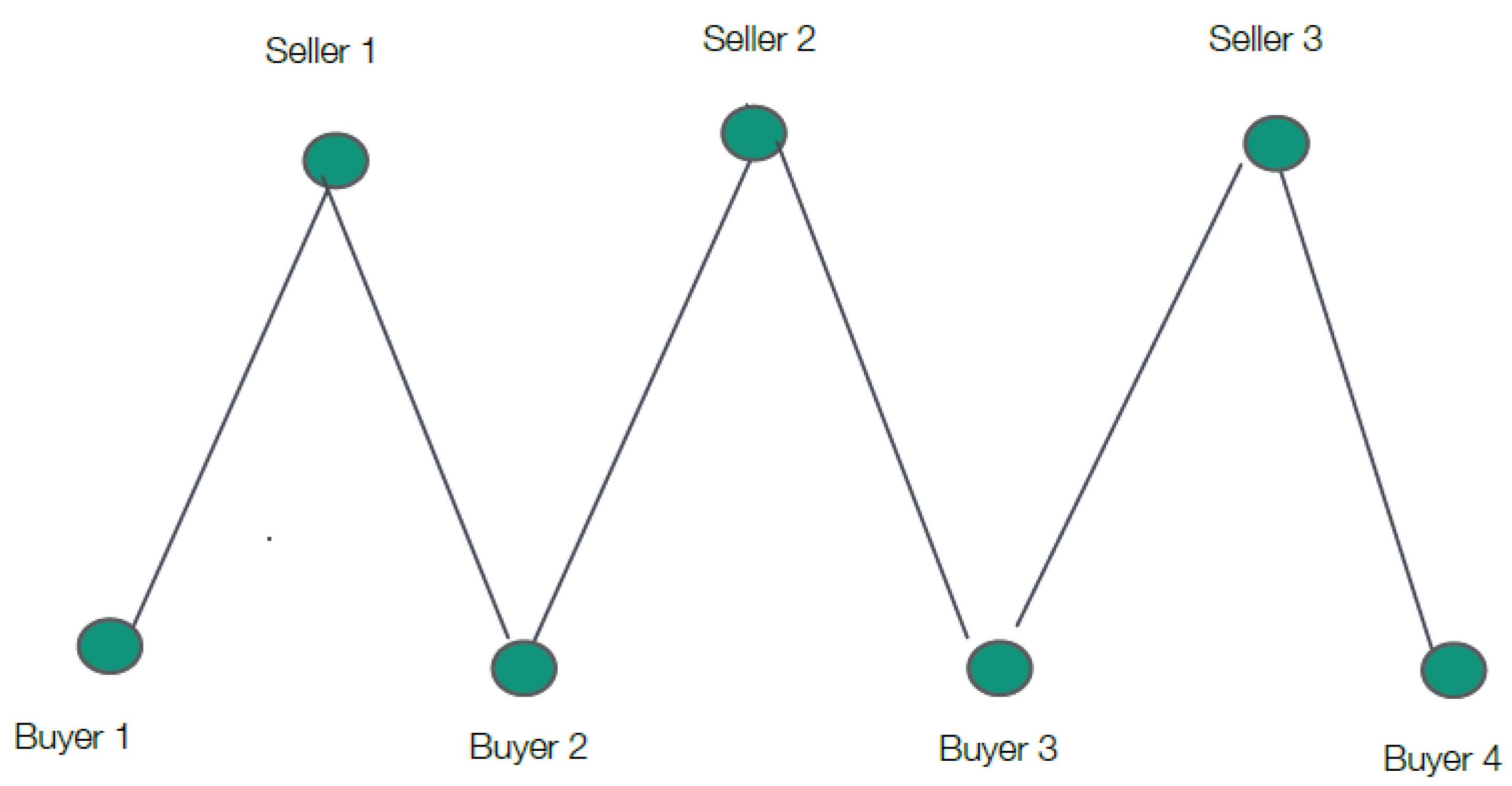
Figure 2.
Buyer-seller graph with allocatively complete seller 2.

- 2.Sales data for Victoria, Australia from 2–8 March 2015 found 309 auctions versus 357 homes sold in private sales see CoreLogic [6]; Thus, many sellers prefer private sales to auctions. Data obtained by Lusht [7] and Stevenson, Young, and Gurdgiev [8] also show a significant number of private sales versus auctions in real estate auctions occurring in Melbourne and Dublin, respectively.
- 3.Alternatively, Zhang and Zhou [11] consider a mechanism for sharing channels where primary users set quotas based on secondary user’s locations in order to maximize profits.
- 4.Fainmesser [22] considers repeated buyer-seller games played on a network where the threat of a loss of repeated interactions can facilitate cooperation.
- 5.Note that when buyers make their decisions on whether to accept or reject the offer they simply compare their expected payoff from the auction without the seller to their payoff from accepting the offer. Specifically, if seller i makes offers to buyers j and ℓ, then from buyer j’s perspective it does not matter if buyer ℓ accepts or rejects i’s offer as either way the auction will take place over . Thus, an assumption of buyers’ myopia is not necessary as buyers do not need to take into account other buyers accepting or rejecting the offer when they make their own decisions.
- 6.The calculation for is given in Example 1. And , where is the probability that .
© 2016 by the author; licensee MDPI, Basel, Switzerland. This article is an open access article distributed under the terms and conditions of the Creative Commons Attribution (CC-BY) license (http://creativecommons.org/licenses/by/4.0/).
Share and Cite
MDPI and ACS Style
Watts, A. Auctions Versus Private Negotiations in Buyer-Seller Networks. Games 2016, 7, 22. https://doi.org/10.3390/g7030022
AMA Style
Watts A. Auctions Versus Private Negotiations in Buyer-Seller Networks. Games. 2016; 7(3):22. https://doi.org/10.3390/g7030022
Chicago/Turabian StyleWatts, Alison. 2016. "Auctions Versus Private Negotiations in Buyer-Seller Networks" Games 7, no. 3: 22. https://doi.org/10.3390/g7030022
Note that from the first issue of 2016, this journal uses article numbers instead of page numbers. See further details here.