Multidimensional Screening with Complementary Activities: Regulating a Monopolist with Unknown Cost and Unknown Preference for Empire Building

Abstract

We study the optimal regulation of a monopolist when intrinsic efficiency (intrinsic cost) and empire building tendency (marginal utility of output) are private information, but actual cost (the difference between intrinsic cost and effort level) is observable. This is a problem of multidimensional screening with complementary activities. Results are not only driven by the prior probabilities of the four possible types, but also by the relative magnitude of the uncertainty along the two dimensions of private information. If the marginal utility of output varies much more (less) across managers than the intrinsic marginal cost, there is empire building (efficiency) dominance. In that case, an inefficient empire builder produces more (less) and at lower (higher) marginal cost than an efficient money-seeker. It is only when variabilities are similar that there may be the natural ranking of activities (empire builders produce more, while efficient managers produce at a lower cost).

1. Introduction

Armstrong and Rochet [1] have provided a “user’s guide” for studying multidimensional screening problems.1 They studied a model with two activities, focusing on the case in which the utility functions of the agent and of the principal are additively separable in the levels of the two activities (independent activities). Furthermore, they considered that the agent’s types are defined by two parameters coming from a binary distribution, with each parameter corresponding to one of the activities, in the sense that it only influences the utility of the agent and of the principal that is associated with that activity. They provided a full solution for this setup and concluded that the qualitative properties of the solution are determined by the correlation between the two parameters and by the amount of “symmetry” between the two activities.

The methodology proposed by Armstrong and Rochet [1] is the following: (i) start by considering a relaxed problem where only the downward incentive-compatibility constraints are accounted for; (ii) solve this relaxed problem; and (iii) find conditions that ensure that the solution of the relaxed problem is the solution of the fully constrained one. They noted, however, that it may be the case that upward or diagonal constraints bind and outlined the resulting equilibria (in that case, activities may be distorted upward and not only downward).

We consider here a somewhat different problem. We start from the well-known model of Laffont and Tirole [3], which deals with the regulation of a monopolist that has private information about his/her intrinsic marginal cost. In this model, the manager of the firm chooses a level of effort, which decreases the marginal cost of production, but is costly to the manager. The effort level is also private information of the manager, but the regulator observes the resulting production cost. Borges and Correia-da-Silva [4] modified this framework by assuming that the manager may have a preference for empire building, i.e., may have a positive marginal utility for output (or employment, if we assume that employment determines output via a deterministic production function).2 They showed that the regulator’s welfare is increasing with the manager’s tendency for empire building: the more the manager is interested in a non-monetary reward, the lower is the monetary informational rent he/she requires. In a subsequent paper, Borges, Correia-da-Silva and Laussel [9] studied the case in which the magnitude of the tendency for empire building is private information of the manager, while the intrinsic marginal cost is observable. Here, we study the case in which the private information of the manager bears simultaneously on the value of the intrinsic marginal cost and on the value of the marginal utility of output. This leads to a two-dimensional screening model with complementary activities.

We suppose that both the level of efficiency and the tendency for empire building can be either high or low (the intrinsic marginal cost and the marginal utility of output are drawn from a binary distribution). There are, therefore, four types of managers: the efficient money-seeker, the efficient empire builder, the inefficient money-seeker and the inefficient empire builder. The resulting problem differs from the one considered by Armstrong and Rochet [1], because the utility function of the regulator is not separable in the two activities—output and effort are complementary. More precisely, since effort reduces the marginal cost of output, more effort yields a larger optimal output level. In turn, a larger output level increases the returns from any given effort level and, thus, leads to a larger optimal effort level.

Our purpose is twofold. First, it is a substantive one: we aim at analyzing the characteristics of optimal contracts between regulator and manager in the two-dimensional case, where the manager’s preference for high output is private information, as well as his/her intrinsic efficiency. Second, it is a methodological one: we want to see how the method proposed by Armstrong and Rochet [1] performs in the case of complementary activities.3

When analyzing our model, we realized that the approach of Armstrong and Rochet [1] did not provide a complete picture of the possible kinds of solutions. In fact, the solutions of the relaxed problem obtained by considering only the downward incentive constraints (and ignoring the upward and diagonal incentive constraints)4 rarely solve the fully constrained problem, and finding general conditions for that seems to be very hard. More precisely, with complementary activities, the diagonal constraints are frequently binding. This is why our approach is based on the consideration of a less relaxed problem, where only the upward incentive compatibility constraints are discarded. Inclusion of the diagonal incentive constraints increases the number of a priori possible combinations of binding and non-binding incentive constraints to 63, which means that the analysis is much more difficult and tedious.

One of our main findings is that an important determinant of the kind of solution that is obtained is the ratio between the variability (across managers) of the marginal utility of output and the variability of intrinsic efficiency. When these variabilities are very different, the model becomes similar to a one-dimensional model, where the relevant private information concerns the dimension in which managers differ in a greater degree. Since Armstrong and Rochet [1] showed that the correlation between types is the main driver of the kind of solution that is obtained when activities are independent, our results suggest that, when activities are complementary, there is another element that significantly drives the results: the relative magnitude of the uncertainty along each dimension of private information.

When intrinsic efficiency varies much more than marginal utility of output, there is “efficiency dominance”: more efficient managers have lower marginal cost and larger output levels than the less efficient ones (an efficient money-seeker produces more than an inefficient manager). When it is large, there is “empire building dominance”: manager types with a stronger tendency for empire building types have larger output and lower marginal cost levels than managers with a weaker tendency for empire building (an inefficient empire builder exerts more effort than an efficient money-seeker).

Assuming that the variabilities of efficiency and the tendency for empire building are equal, we find three kinds of solutions: (i) output bunching between the money-seekers and marginal cost bunching between the inefficient managers; (ii) output bunching between the inefficient empire builder and the efficient money-seeker; and (iii) natural ranking of activities, i.e., more efficient types producing at lower marginal cost, types with a stronger tendency for empire building producing more output.

The rest of the paper is organized as follows. Section 2 introduces the model and the multidimensional screening problem. Section 3 focuses on a relaxed problem. Section 4 presents the solutions to several cases that differ qualitatively. Section 5 concludes the paper with some remarks. The systems of equations that characterize each case and the proofs of the formal results are presented in the Appendix.

2. The Model

The firm produces an observable quantity of a good, $q\ge 0$, with an observable total cost, $C=(\beta -e)q$, where β is the intrinsic marginal cost of the manager and e is the level of effort that is exerted by the manager. Neither the intrinsic marginal cost, β, nor the effort level, e, are directly observable, but the marginal cost can be inferred: $c=\beta -e=C/q$.

The regulator pays the observed production cost plus a net transfer, t, to the manager. The manager attributes utility to this monetary reward and, also, to output in itself. The utility of the manager is:

$$U=t-\psi \left(e\right)+\delta q=t-\psi (\beta -c)+\delta q,$$

where $\psi \left(e\right)$ is the disutility of effort, assumed to be a convex function, and δ is the marginal utility of output.

The marginal utility of output is the private information of the manager (as well as the intrinsic marginal cost). It measures the importance of the empire building component of the manager’s utility. A positive value of δ means that the manager likes to produce a higher output, or, for example, to have authority over more employees.

The manager requires a minimum utility level (which we set to zero for convenience) to accept the contract. The participation constraint is: $U\ge 0$.

A level of output equal to q generates a consumer surplus that is given by $S\left(q\right)$. Social welfare is measured as the difference between the total surplus (consumer surplus plus firm surplus) and the cost of raising funds to compensate the firm, $(1+\lambda )(C+t)$, with $\lambda >0$:

$$\begin{array}{lll}W& =& S\left(q\right)-(1+\lambda )(C+t)+U,\\ & =& S\left(q\right)-(1+\lambda )\left[cq+\psi (\beta -c)-\delta q\right]-\lambda U.\end{array}$$

Notice that the regulator’s welfare is increasing with the manager’s marginal utility of output, because, when the manager enjoys more of a given level of output, this reduces the money transfer that is necessary to compensate him/her. It obviously follows that, other things being equal (and, specifically, the intrinsic cost, β), the regulator prefers an empire builder to a pure money-seeker.

There are two possible values of β, namely ${\beta }_E<{\beta }_I$, and two possible values of δ, namely ${\delta }_M<{\delta }_B$. There are, then, four possible types of managers: the efficient money-seeker, $({\beta }_E,{\delta }_M)$; the efficient empire builder, $\left({\beta }_E,{\delta }_B\right)$; the inefficient money-seeker, $\left({\beta }_I,{\delta }_M\right)$; and the inefficient empire builder, $\left({\beta }_I,{\delta }_B\right)$.

Obviously, the efficient empire builder ($EB$) is the best type for the principal, and the inefficient money-seeker ($IM$) is the worst type. It is also clear that $EB$ is a better type than the inefficient empire builder ($IB$) and the efficient money-seeker ($EM$); and that $IB$ and $EM$ are better types than $IM$. It is not possible to rank a priori the two intermediate types, i.e., $IB$ and $EM$.

Let $\omega \equiv \frac{{\delta }_B-{\delta }_M}{{\beta }_I-{\beta }_E}$ be the relative variability of empire building tendency and efficiency (among the different types). We will see that many results are driven by the value of this parameter.

The prior probabilities associated with the manager types are ${\alpha }_{EB},{\alpha }_{EM},{\alpha }_{IB}$ and ${\alpha }_{IM}$, all assumed to be strictly positive. The vector of prior probabilities is denoted by $\alpha \equiv \left({\alpha }_{EB},{\alpha }_{EM},{\alpha }_{IB},{\alpha }_{IM}\right)$. It is also useful to define $\rho \equiv 1-\frac{{\alpha }_{EM}{\alpha }_{IB}}{{\alpha }_{EB}{\alpha }_{IM}}$, which we will refer to as the “correlation” between efficiency and empire building.

The regulator maximizes:

$$\sum _{i=\left\{E,I\right\}}\sum _{j=\left\{M,B\right\}}{\alpha }_{ij}{W}_{ij},$$

where $W_{ij}=S\left(q_{ij}\right)-(1+\lambda )\left[c_{ij}{q}_{ij}+\psi ({\beta }_i-c_{ij})-{\delta }_j{q}_{ij}\right]-\lambda U_{ij}$.

It is very important to notice that, from the regulator’s point of view, the two activities, output and efficiency, are complements, i.e., $\frac{{\partial }^2{W}_{ij}}{\partial q_{ij}\partial c_{ij}}=-(1+\lambda )<0$. Higher efficiency makes a larger output level more desirable and vice versa. This is a substantial difference with respect to the setup of Armstrong and Rochet [1], where both the agent and the principal have additively separable utility functions.

The regulator offers a menu of contracts to the manager, such that the manager of type $ij$ produces $q_{ij}$ at marginal cost $c_{ij}$ and receives a net transfer $t_{ij}$, which results in a utility level $U_{ij}$. In this problem, there are four participation constraints and twelve incentive constraints.

The only binding participation constraint is $U_{IM}\ge 0$, because it implies that all the other types are able to attain a strictly positive utility level. The inefficient money-seeker (worst type) obtains its reservation utility.

The incentive constraints may be downward, upward or diagonal. The downward (upward) constraints are those in which the constrained type is better (worse) than the constraining type in both dimensions. In the diagonal constraints, each of the types is better in one dimension and worse in the other.

The incentive constraint that imposes that the constrained type, $ij$, cannot be better off by mimicking the constraining type, $i^{\prime }{j}^{\prime }$, will be denoted constraint $ij/i^{\prime }{j}^{\prime }$. There are five downward constraints ($EB/IM$, $EB/EM$, $EB/IB$, $EM/IM$ and $IB/IM)$, five upward constraints ($IM/EB$, $EM/EB$, $IB/EB$, $IM/EM$ and $IM/IB$) and two diagonal constraints ($EM/IB$ and $IB/EM$).

A manager of type $ij$ that claims to be of type $i^{\prime }{j}^{\prime }$ obtains the utility level of type $i^{\prime }{j}^{\prime }$, plus the difference in the empire building component of utility, $({\delta }_j-{\delta }_{j^{\prime }})q_{i^{\prime }{j}^{\prime }}$, and minus the difference in the disutility of the effort component, $\psi ({\beta }_i-c_{i^{\prime }{j}^{\prime }})-\psi ({\beta }_{i^{\prime }}-c_{i^{\prime }{j}^{\prime }})$. The corresponding incentive compatibility constraint ($ij/i^{\prime }{j}^{\prime }$) is:

$$U_{ij}\ge U_{i^{\prime }{j}^{\prime }}+({\delta }_j-{\delta }_{j^{\prime }})q_{i^{\prime }{j}^{\prime }}+\psi ({\beta }_{i^{\prime }}-c_{i^{\prime }{j}^{\prime }})-\psi ({\beta }_i-c_{i^{\prime }{j}^{\prime }}).$$

(1)

The following monotonicity property is a direct consequence of the incentive constraints.

Remark 1. An empire builder produces more output than a money-seeker (with the same efficiency), and an efficient manager produces with a lower cost than an inefficient manager (with the same tendency for empire building):

$$\begin{array}{l}{q}_{iB}\ge q_{iM},\forall i\in \left\{E,I\right\},\end{array}$$

(2a)

$$\begin{array}{l}{c}_{Ej}\le c_{Ij},\forall j\in \left\{M,B\right\}.\end{array}$$

(2b)

Proof. Adding the two incentive constraints between types $ij$ and $i^{\prime }{j}^{\prime }$, we obtain: $0\ge ({\delta }_j-{\delta }_{j^{\prime }})(q_{i^{\prime }{j}^{\prime }}-q_{ij})+\psi ({\beta }_{i^{\prime }}-c_{i^{\prime }{j}^{\prime }})-\psi ({\beta }_i-c_{i^{\prime }{j}^{\prime }})+\psi ({\beta }_i-c_{ij})-\psi ({\beta }_{i^{\prime }}-c_{ij})$. Considering types $iB$ and $iM$, we obtain $0\ge ({\delta }_B-{\delta }_M)(q_{iM}-q_{iB})$, which implies that $q_{iB}\ge q_{iM}$. Considering types $Ej$ and $Ij$, we obtain $0\ge \psi ({\beta }_I-c_{Ij})-\psi ({\beta }_E-c_{Ij})+\psi ({\beta }_E-c_{Ej})-\psi ({\beta }_I-c_{Ej})$. Since ψ is a convex function, this implies that $c_{Ej}\le c_{Ij}$. ☐

We will focus on the case in which $\psi \left(e\right)=\frac{e^2}{2}$ and $S\left(q\right)=2q-q^2$. To ensure that the problem is concave, we also assume that $\lambda <1$.5 In this case, the incentive constraints can be written as:

$$U_{ij}\ge U_{i^{\prime }{j}^{\prime }}+({\delta }_j-{\delta }_{j^{\prime }})q_{i^{\prime }{j}^{\prime }}+\frac{1}{2}({\beta }_{i^{\prime }}^2-{\beta }_i^2)+c_{i^{\prime }{j}^{\prime }}({\beta }_i-{\beta }_{i^{\prime }}),$$

(3)

for all $ij$ and $i^{\prime }{j}^{\prime }$.

Denote by $q_{ij}^{*}$ and $c_{ij}^{*}$ the perfect information output and marginal cost for each manager type. The first-order conditions are:

$$\begin{array}{ccc}\hfill S^{\prime }\left(q_{ij}^{*}\right)& =& (1+\lambda )\left(c_{ij}^{*}-{\delta }_i\right),\hfill \\ \hfill {\psi }^{\prime }({\beta }_i-c_{ij}^{*})& =& q_{ij}^{*}.\hfill \end{array}$$

Since $\psi \left(e\right)=\frac{e^2}{2}$ and $S\left(q\right)=2q-q^2$, the first-best solution (perfect information benchmark) is:

$$\begin{array}{lll}& & q_{ij}^{*}=\frac{1}{1-\lambda }\left[2-({\beta }_i-{\delta }_j)(1+\lambda )\right],\\ & & c_{ij}^{*}=\frac{1}{1-\lambda }\left[-2+2{\beta }_i-(1+\lambda ){\delta }_j\right].\end{array}$$

The above expressions illustrate the complementarity between output and efficiency, which is the main characteristic of the model. For instance, a high value of the marginal utility of output translates not only into a high first-best output level, but also into a high first-best efficiency level. Reciprocally, a low value of the intrinsic marginal cost translates not only into a high level of efficiency, but also into a high output level. It is not true, contrary to a model with separable utility functions, that intrinsically efficient managers always exhibit first-best efficiency levels and more output-oriented managers produce their first-best output levels. Due to the complementarity property, downward distortions along one dimension result in downward distortions along the other dimension.

The complementarity of activities seriously complicates the analysis of the model. Armstrong and Rochet [1], when analyzing the case of independent activities, considered first a “relaxed” problem obtained by considering only the downward incentive constraints, i.e., by neglecting the upward incentive constraints and the two diagonal incentive constraints (those between the two intermediate types). In a second stage, they checked that the neglected constraints were indeed satisfied by the solutions of the relaxed problem (or found conditions that ensured that they were satisfied). When activities are complementary, the solutions of such a relaxed problem almost never satisfy the diagonal constraints. This is why we consider a less relaxed problem, where only the upward constraints are discarded.

3. The Relaxed Problem

We define a relaxed problem in which only the downward and the diagonal incentive constraints are considered, together with the participation constraint for the worst type (the only one that is binding):

$$\underset{q,c,U}{\max }\sum _{(i,j)}{\alpha }_{ij}\left\{S\left(q_{ij}\right)-(1+\lambda )\left[\left(c_{ij}-{\delta }_j\right)q_{ij}+\psi ({\beta }_i-c_{ij})\right]-\lambda U_{ij}\right\}$$

subject to:

$$\begin{array}{ccc}\hfill U_{IM}& =& 0,\hfill \end{array}$$

(4a)

$$\begin{array}{ccc}\hfill U_{EB}& \ge & U_{EM}+\Delta \delta q_{EM},\hfill \end{array}$$

(4b)

$$\begin{array}{ccc}\hfill U_{EB}& \ge & U_{IB}-\Delta \beta c_{IB}+k,\hfill \end{array}$$

(4c)

$$\begin{array}{ccc}\hfill U_{EB}& \ge & \Delta \delta q_{IM}-\Delta \beta c_{IM}+k,\hfill \end{array}$$

(4d)

$$\begin{array}{ccc}\hfill U_{IB}& \ge & \Delta \delta q_{IM},\hfill \end{array}$$

(4e)

$$\begin{array}{ccc}\hfill U_{EM}& \ge & -\Delta \beta c_{IM}+k,\hfill \end{array}$$

(4f)

$$\begin{array}{ccc}\hfill U_{IB}& \ge & U_{EM}+\Delta \delta q_{EM}+\Delta \beta c_{EM}-k,\hfill \end{array}$$

(4g)

$$\begin{array}{ccc}\hfill U_{EM}& \ge & U_{IB}-\Delta \beta c_{IB}+k-\Delta \delta q_{IB},\hfill \end{array}$$

(4h)

where $\Delta \beta \equiv {\beta }_I-{\beta }_E$, $k\equiv \frac{1}{2}\left({\beta }_I^2-{\beta }_E^2\right)$ and $\Delta \delta \equiv {\delta }_B-{\delta }_M$.

The solution of the relaxed problem must be such that:

$$\begin{array}{ccc}\hfill U_{IB}& =& \max \left\{\Delta \delta q_{IM};U_{EM}+\Delta \delta q_{EM}+\Delta \beta c_{EM}-k\right\},\hfill \end{array}$$

(5a)

$$\begin{array}{ccc}\hfill U_{EM}& =& \max \left\{-\Delta \beta c_{IM}+k;U_{IB}-\Delta \beta c_{IB}+k-\Delta \delta q_{IB}\right\},\hfill \end{array}$$

(5b)

$$\begin{array}{ccc}\hfill U_{EB}& =& \max \left\{U_{EM}+\Delta \delta q_{EM};U_{IB}-\Delta \beta c_{IB}+k;\Delta \delta q_{IM}-\Delta \beta c_{IM}+k\right\}.\hfill \end{array}$$

(5c)

Equations (5a) and (5b) are the incentive constraints of the intermediate types ($IB$ and $EM$). For each of them, the constraining type that binds may be the other intermediate type, the worst type or both. Equation (5c) is the best type’s incentive constraint: $EB$ may indeed be constrained by $IB$, $EM$, $IM$ or by two or three of them (seven possibilities). Combining the possible solutions of (5), there are up to 63 possible patterns of binding incentive constraints.

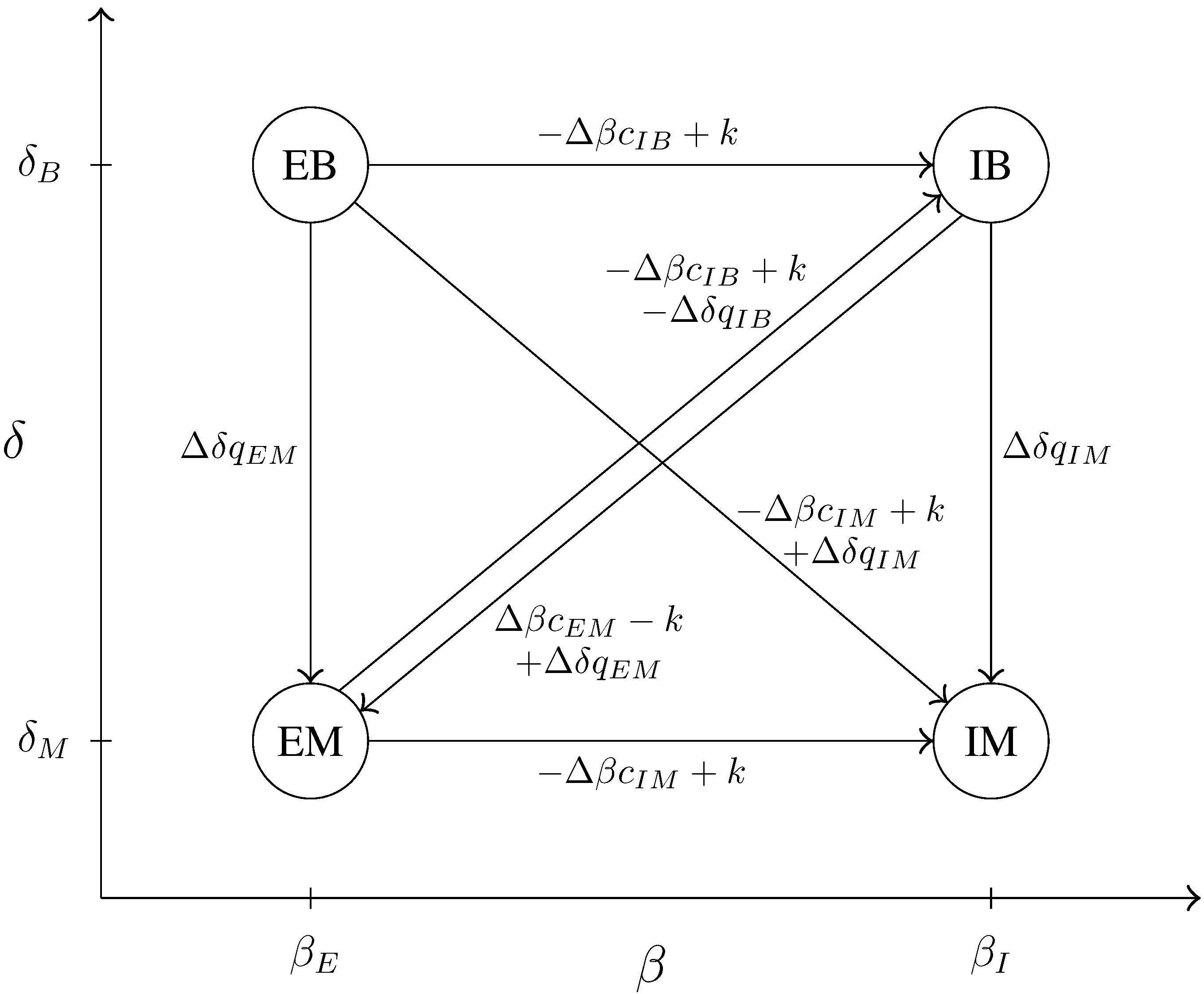
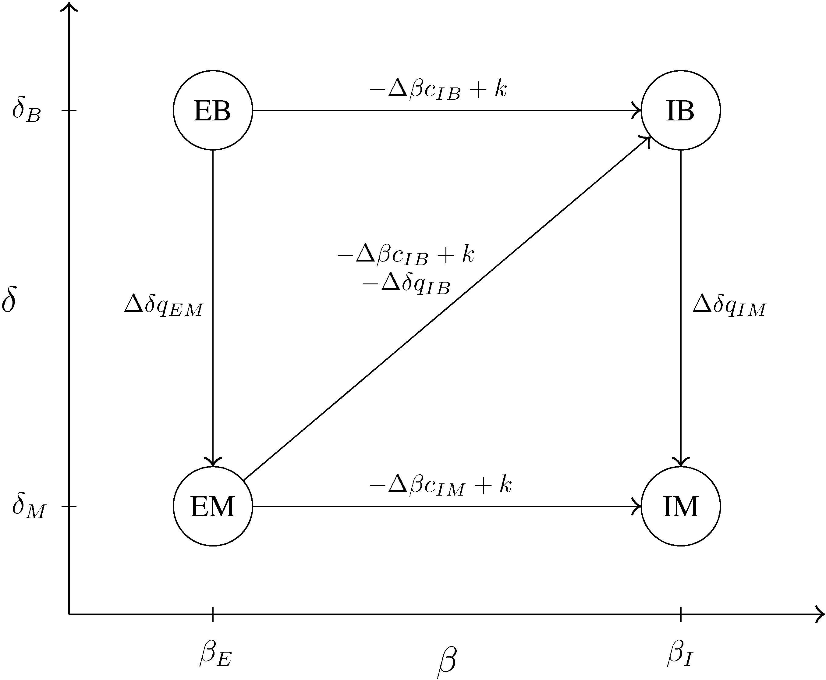
Figure 1 pictures all the possibly binding downward and diagonal incentive constraints. Notice that types on the left are intrinsically more efficient, and types above are more output-oriented. It should be read as follows. The arrow starting from $EB$ and going to $IB$ represents the downward constraint, $EB/IB$: the difference between $U_{EB}$ and $U_{IB}$ must be at least equal to $-\Delta \beta c_{IB}+k$. Consider the arrow from $EM$ to $IB$: the difference between $U_{EM}$ and $U_{IB}$ must be at least $-\Delta \beta c_{IB}+k-\Delta \delta q_{IB}$.

Figure 1. Downward and diagonal incentive constraints.

Figure 1. Downward and diagonal incentive constraints.

To determine which of the constraints are binding, one has to compare the “lengths” of the paths from a point, $ij$, to another, $i^{\prime }{j}^{\prime }$. Constraints are non-binding if there is a longer path between the two points. For instance, to go from $EB$ to $IM$, there are three possible paths: $EB/IM$, $EB/IB$ + $IB/IM$ and $EB/EM$ + $EM/IM$. To determine which is the longest, one has to compare $\Delta \delta q_{IM}-\Delta \beta c_{IM}+k$, $\Delta \delta q_{IM}-\Delta \beta c_{IB}+k$ and $\Delta \delta q_{EM}-\Delta \beta c_{IM}+k$. To go from $EM$ to $IM$, there are two possible paths: $EM/IM$ and $EM/IB$ + $IB/IM$, and so on.

Let ${\gamma }_1$ to ${\gamma }_5$ be the non-negative Lagrange multipliers associated with the five downward constraints ($EB/EM$, $EB/IB$, $EB/IM$, $IB/IM$ and $EM/IM$, respectively) and ${\gamma }_6$ and ${\gamma }_7$ the multipliers associated with the diagonal constraints ($IB/EM$ and $EM/IB$, respectively).

The first-order conditions with respect to $U_{EB}$, $U_{EM}$ and $U_{IB}$ are:

$$\begin{array}{lll}-\lambda {\alpha }_{EB}+{\gamma }_1+{\gamma }_2+{\gamma }_3& =& 0,\end{array}$$

(6a)

$$\begin{array}{lll}-\lambda {\alpha }_{EM}-{\gamma }_1+{\gamma }_5-{\gamma }_6+{\gamma }_7& =& 0,\end{array}$$

(6b)

$$\begin{array}{lll}-\lambda {\alpha }_{IB}-{\gamma }_2+{\gamma }_4+{\gamma }_6-{\gamma }_7& =& 0.\end{array}$$

(6c)

For $S\left(q\right)=2q-q^2$ and $\psi \left(e\right)=\frac{e^2}{2}$, the first-order conditions with respect to $q_{ij}$ and $c_{ij}$ yield:6

$$\begin{array}{ccc}\hfill q_{EB}& =& \frac{1}{1-\lambda }\left[2-(1+\lambda )({\beta }_E-{\delta }_B)\right],\hfill \end{array}$$

(7a)

$$\begin{array}{ccc}\hfill q_{EM}& =& \frac{1}{1-\lambda }\left[2-(1+\lambda )({\beta }_E-{\delta }_M)-\frac{({\gamma }_1+{\gamma }_6)\Delta \delta -{\gamma }_6\Delta \beta }{{\alpha }_{EM}}\right],\hfill \end{array}$$

(7b)

$$\begin{array}{ccc}\hfill q_{IB}& =& \frac{1}{1-\lambda }\left[2-(1+\lambda )({\beta }_I-{\delta }_B)-\frac{({\gamma }_2+{\gamma }_7)\Delta \beta -{\gamma }_7\Delta \delta }{{\alpha }_{IB}}\right],\hfill \end{array}$$

(7c)

$$\begin{array}{ccc}\hfill q_{IM}& =& \frac{1}{1-\lambda }\left[2-(1+\lambda )({\beta }_I-{\delta }_M)-\frac{\left({\gamma }_3+{\gamma }_4\right)\Delta \delta +({\gamma }_3+{\gamma }_5)\Delta \beta }{{\alpha }_{IM}}\right],\hfill \end{array}$$

(7d)

$$\begin{array}{ccc}\hfill c_{EB}& =& \frac{1}{1-\lambda }\left[-2+2{\beta }_E-(1+\lambda ){\delta }_B\right],\hfill \end{array}$$

(7e)

$$\begin{array}{ccc}\hfill c_{EM}& =& \frac{1}{1-\lambda }\left[-2+2{\beta }_E-(1+\lambda ){\delta }_M+\frac{({\gamma }_1+{\gamma }_6)\Delta \delta -{\gamma }_6\frac{2\Delta \beta }{1+\lambda }}{{\alpha }_{EM}}\right],\hfill \end{array}$$

(7f)

$$\begin{array}{ccc}\hfill c_{IB}& =& \frac{1}{1-\lambda }\left[-2+2{\beta }_I-(1+\lambda ){\delta }_B+\frac{({\gamma }_2+{\gamma }_7)\frac{2\Delta \beta }{1+\lambda }-{\gamma }_7\Delta \delta }{{\alpha }_{IB}}\right],\hfill \end{array}$$

(7g)

$$\begin{array}{ccc}\hfill c_{IM}& =& \frac{1}{1-\lambda }\left[-2+2{\beta }_I-(1+\lambda ){\delta }_M+\frac{\left({\gamma }_3+{\gamma }_4\right)\Delta \delta +({\gamma }_3+{\gamma }_5)\frac{2\Delta \beta }{1+\lambda }}{{\alpha }_{IM}}\right].\hfill \end{array}$$

(7h)

Besides the classical “no distortion at the top” (i.e., for the efficient empire builder), what we mainly observe in these results is that the distortion of the activities of type $ij$ decrease with the probability, ${\alpha }_{ij}$, associated with his/her type. On the other hand, it increases with the probability of type $i^{\prime }{j}^{\prime }$ if the corresponding incentive constraint, $i^{\prime }{j}^{\prime }/ij$, is binding. Finally, a distortion along the intrinsic efficiency dimension effects not only the cost level, but also the output level and, reciprocally, for a distortion along the empire building dimension.

It is not surprising that the efficient empire builder ($EB$) must produce more and at a lower marginal cost than the inefficient money-seeker ($IM$).

Remark 2. In any solution of the relaxed problem, we have:

$$\begin{array}{l}{q}_{EB}>q_{IM},c_{EB}<c_{IM}and{e}_{EB}<e_{IM}.\end{array}$$

Proof. It follows from (7a), (7e), (7d) and (7h), given the non-negativity of the multipliers.  ☐

After finding the solution of the relaxed problem, we will be interested in checking that the upward incentive constraints are satisfied. The next result is helpful for that purpose.

Remark 3. If a downward incentive constraint is binding, the corresponding upward incentive constraint is surely satisfied if the activity levels satisfy the monotonicity property (2).

Proof. See Appendix 6.1. ☐

Notice that, while Remark 1 establishes that the monotonicity property is a consequence of the incentive constraints, Remark 3 establishes that each upward incentive constraint is a consequence of the monotonicity property and of the corresponding downward incentive constraint.

4. Several Possible Scenarios

In this section, we analyze possible solutions of the relaxed problem and of the fully constrained problem. The methodology that we use is the following. We start by assuming that the incentive constraints that are binding are those that belong to a certain set. This set defines what is called a Case. Then, for each Case, i.e., taking as given the list of binding and non-binding incentive constraints, a solution candidate (output, cost and utility for each type and values of the Lagrange multipliers) is computed from the first-order conditions, (6) and (7), and from the incentive constraints, (4). While the binding incentive constraints provide additional equations, the non-binding incentive constraints allow us to set the corresponding multipliers to zero. Finally, we study the conditions under which the solution candidate obtained in each Case is an actual solution of the relaxed problem and of the fully constrained problem. To be a solution of the relaxed problem, it is necessary that the values of the multipliers associated with the binding incentive constraints are non-negative. If they are, we say that the Case is optimal in the relaxed problem. To be a solution of the fully constrained problem, it is also necessary that the upward incentive constraints are satisfied. If they are, we say that the Case is optimal in the relaxed problem and in the fully constrained problem.

The number of possible cases is a priori very large, so it is almost impossible to study all of them. Only a few of them lead to activity levels that solve the principal’s problem for some set of parameter values. We present some of these cases, focusing on the importance of $\omega =\frac{\Delta \delta }{\Delta \beta }$ in determining the nature of the solutions.

4.1. Case A: Low Probabilities of Intermediate Types

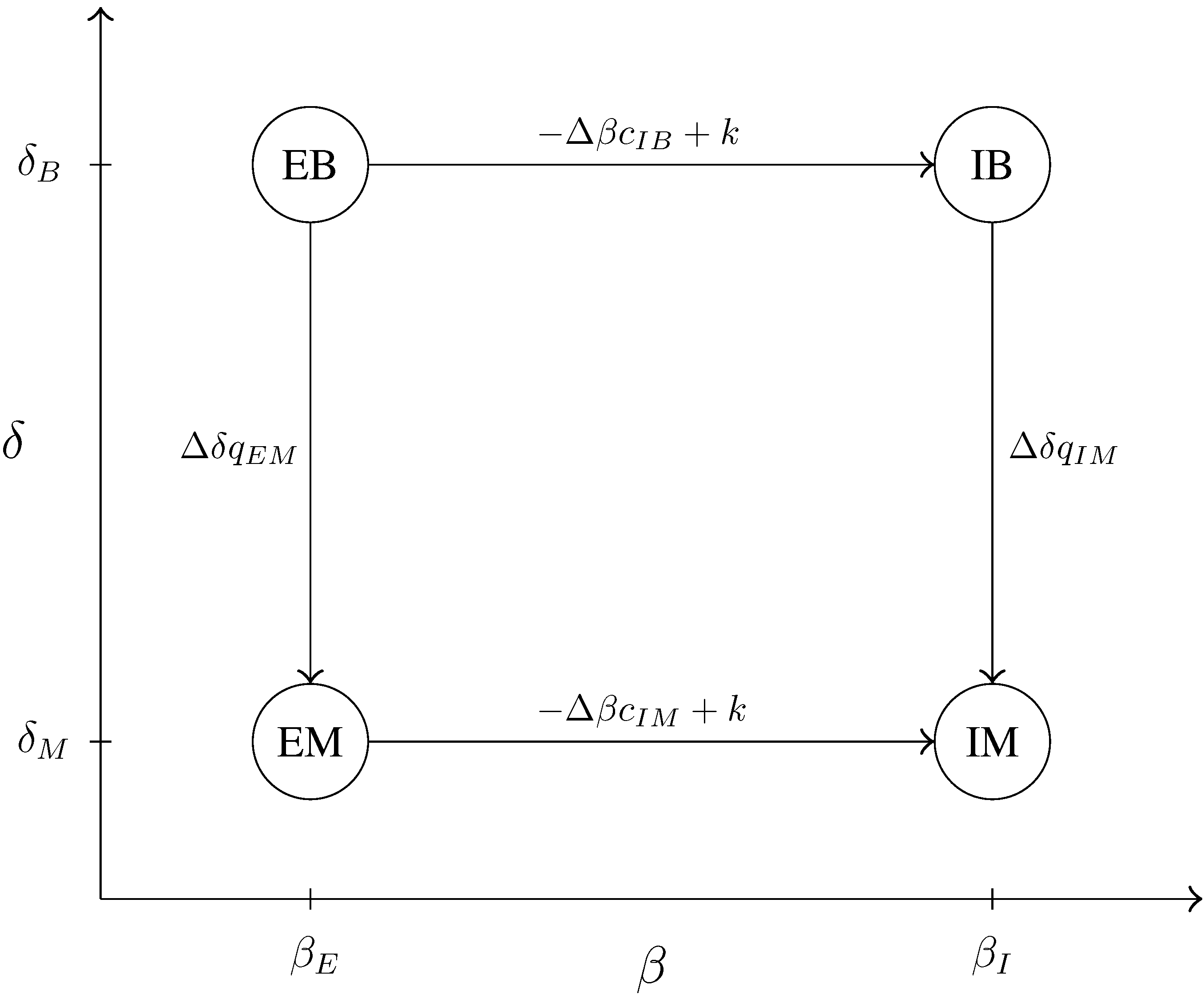
We start with the first case that was presented by Armstrong and Rochet [1]. In this case, all the downward constraints are binding, while the diagonal constraints are not binding.

The solution of the fully constrained problem is of this kind when the probabilities of the two intermediate types are low.

In this case, there is a bunching of the output levels of the money-seekers ($q_{EM}=q_{IM}$) and a bunching of the cost levels of the inefficient managers ($c_{IB}=c_{IM}$). Besides that, the ranking of the activity levels is “natural”, in the sense that: the ranking of the output is primarily determined by the preference for the output, while the ranking of the observed efficiency is primarily determined by the intrinsic efficiency.

Remark 4. When Case A is optimal in the relaxed problem, output and marginal cost levels are ranked in the natural way, with a bunching of the worst types in each activity:

$$\begin{array}{l}{q}_{EB}>q_{IB}\ge q_{EM}=q_{IM},\\ c_{EB}<c_{EM}\le c_{IB}=c_{IM}.\end{array}$$

Figure 2. Incentive constraints that are binding in Case A.

Figure 2. Incentive constraints that are binding in Case A.

Proof. See Appendix 6.2. ☐

The solution of the relaxed problem that is obtained in Case A is also the solution of the fully constrained problem if the probabilities of the types that are favorable in one dimension and unfavorable in the other are below a certain threshold.

Proposition 1. Case A is optimal in the relaxed problem and in the fully constrained problem if $\min \left\{{\alpha }_{EM},{\alpha }_{IB}\right\}<{\alpha }^{*}$, where ${\alpha }^{*}$ is a strictly positive function of the remaining parameters.

Proof. See Appendix 6.2. ☐

4.2. Cases B and C: Equal Variabilities of β and δ

Several cases can only occur if ω is equal to one. In these cases, the ranking of types is not primarily determined by their ranking along a single dimension (there is neither “empire building dominance” nor “efficiency dominance”).

In Case B, which occurs when the “correlation” between empire building and efficiency is not too negative and when the probability of the worst type is intermediate, the ranking of managers according to their preference for the output determines the ranking of their output levels, while the ranking of managers according to their intrinsic efficiency determines the ranking of their marginal cost levels. In this case, we are close to a model with independent activities. In fact, it coincides with the second of the cases that were analyzed by Armstrong and Rochet [1].

In Case C, which holds when the probability of the worst type is low, the output levels of the inefficient empire builder and the efficient money-seeker are identical (partial bunching). This case did not appear in the work of Armstrong and Rochet [1].

4.2.1. Case B: Natural Ranking of Activity Levels

In Case B, we suppose that the diagonal incentive constraints are not binding, while all the downward constraints, except $EB/IM$, are binding. This case holds when efficiency and tendency for empire building are not too negatively correlated and $\omega =1$.

Figure 3. Incentive constraints that are binding in Case B.

Figure 3. Incentive constraints that are binding in Case B.

There is a natural ranking of activity levels. The ranking of output levels is primarily determined by the tendency for empire building, while the ranking of marginal cost levels is primarily determined by intrinsic efficiency. Types that have a stronger preference for high output produce more, and types that are intrinsically more efficient produce at a lower cost.

Remark 5. When Case B is optimal in the relaxed problem, output and marginal cost levels are ranked in the natural way:

$$\begin{array}{l}{q}_{EB}>q_{IB}\ge q_{EM}\ge q_{IM},\\ c_{EB}<c_{EM}\le c_{IB}\le c_{IM}.\end{array}$$

Proof. See Appendix 6.3. ☐

Case B provides the solution to the fully constrained problem when the variabilities of β and δ are equal, the “correlation” between efficiency and empire building is not too negative and the probability of the worst type is intermediate.

Proposition 2. Case B is optimal in the relaxed problem and in the fully constrained problem when $\omega =1$ if $\rho \ge -\frac{1-\lambda }{1+\lambda }$ and ${\alpha }_{IM}\in \left[{\alpha }_{IM}^{*},{\alpha }_{IM}^{**}\right]$, where ${\alpha }_{IM}^{*}$ and ${\alpha }_{IM}^{**}$ are functions of the remaining parameters. The interval, $\left[{\alpha }_{IM}^{*},{\alpha }_{IM}^{**}\right]$, is non-empty if and only if $\lambda \le {\lambda }^{*}$, where ${\lambda }^{*}$ is a strictly positive function of ${\alpha }_{EB}$ and ${\alpha }_{EM}$.

Proof. See Appendix 6.3. ☐

4.2.2. Case C: Bunching of Intermediate Output Levels

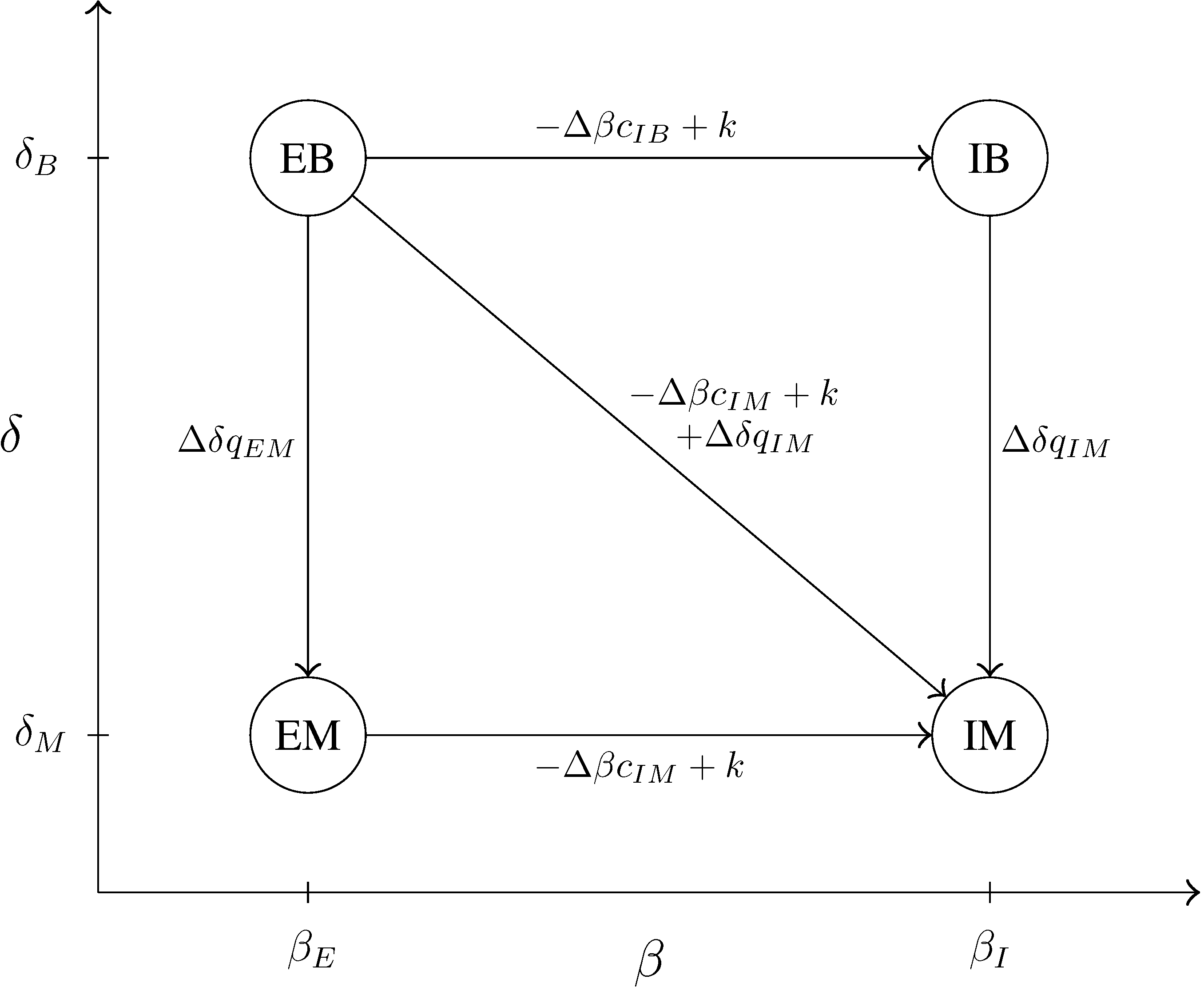
In Case C, we consider the case in which all the (downward and diagonal) incentive constraints are binding, except $EB/IM$ and $IB/EM$.

Figure 4. Incentive constraints that are binding in Case C.

Figure 4. Incentive constraints that are binding in Case C.

Remark 6. When Case C is optimal in the relaxed problem, output and marginal cost levels are ranked as follows:

$$\begin{array}{l}{q}_{EB}>q_{EM}=q_{IB}\ge q_{IM}\\ c_{EB}<c_{EM}<c_{IB}\le c_{IM}.\end{array}$$

Proof. See Appendix 6.4. ☐

There is a bunching of the output levels of the two intermediate types ($q_{EM}=q_{IB}$). On the other hand, there is no bunching of the marginal cost levels ($c_{EM}<c_{IB}$). The efficient money-seeker produces at a lower marginal cost than the inefficient empire builder.

When $\omega =1$, the solution of the original problem is of the kind described in Case C, if and only if the proportion of inefficient money-seekers is sufficiently low.

Proposition 3. Case C is optimal in the relaxed problem and in the fully constrained problem when $\omega =1$ if and only if ${\alpha }_{IM}\le {\alpha }_{IM}^{***}$, where ${\alpha }_{IM}^{***}$ is a strictly positive function of the remaining parameters. ☐

Proof. See Appendix 6.4. ☐

4.3. Case D: Empire Building Dominance ($\Delta \delta \gg \Delta \beta$)

If the variability of the empire building tendency parameter ($\Delta \delta$) is significantly larger than that of the intrinsic marginal cost parameter ($\Delta \beta$), then the inefficient empire builder should be a better type than the efficient money-seeker (because $IB$ has a much stronger empire building tendency and is only slightly less efficient than $EM$). The resulting ordering of types (from the best to the worst) is, then: $EB$, $IB$, $EM$, $IM$.

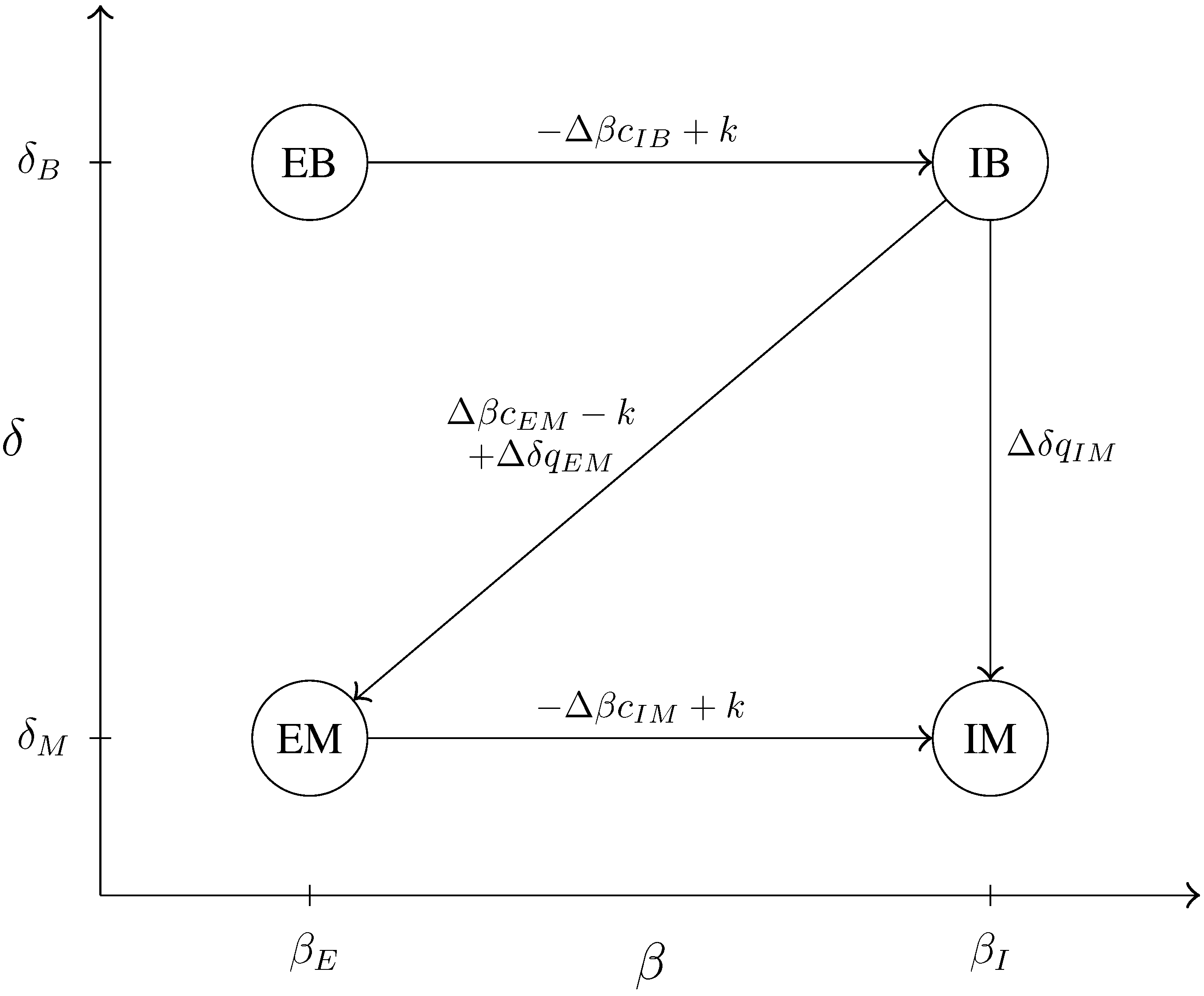
In Case D, the constraints between types that are adjacent according to the ordering mentioned above are binding: the efficient empire builder has to be prevented from mimicking the inefficient empire builder ($EB/IB$), the inefficient empire builder from mimicking the efficient money-seeker ($IB/EM$) and the efficient money-seeker from mimicking the inefficient money-seeker ($EM/IM$). In addition, the constraint that prevents the inefficient empire builder from mimicking the inefficient money-seeker ($IB/IM$) is also binding.

We will show that this corresponds to the solution of the fully constrained problem when ω is sufficiently large.

Output and marginal cost levels are ranked in the same way and primarily according to the tendency of the manager for empire building. An inefficient empire builder produces at lower cost than an efficient money-seeker. This is the intuitive consequence of the complementarity between effort and output. When the variability of the marginal utility of output becomes very large relative to the variability of the intrinsic marginal cost, the greater effort provided by the inefficient empire builder compensates for the lower intrinsic efficiency with respect to the efficient money-seeker.

Remark 7. When Case D is optimal in the fully constrained problem, we must have $\omega >1$ and the following ranking of activity levels:

$$\begin{array}{lll}& & q_{EB}>q_{IB}\ge q_{EM}>q_{IM},\\ & & c_{EB}<c_{IB}\le c_{EM}<c_{IM}.\end{array}$$

Proof. See Appendix 6.5. ☐

Figure 5. Incentive constraints that are binding in Case D.

Figure 5. Incentive constraints that are binding in Case D.

There always exists a threshold value for $\Delta \beta$ below which Case D provides the solution of the original problem.

Proposition 4. Case D is optimal in the relaxed problem and in the fully constrained problem if $\Delta \beta <{\Delta }^{*}$, where ${\Delta }^{*}$ is a strictly positive function of the remaining parameters.

Proof. See Appendix 6.5. ☐

4.4. Case E: Efficiency Dominance ($\Delta \beta \gg \Delta \delta$)

An opposite situation occurs when the variability of the intrinsic marginal cost ($\Delta \beta$) is significantly larger than that of the marginal utility of output ($\Delta \delta$). In that case, $EM$ is a better type than $IB$, because $EM$ is much more efficient and only a slightly less empire builder than $IB$. The intuitive ordering of types, from the best to the worst, is: $EB$, $EM$, $IB$, $IM$.

In Case E, we assume that the binding constraints are those between adjacent types in the above sense ($EB/EM$, $EM/IB$, $IB/IM$) and the one that prevents the efficient money-seeker from mimicking the inefficient money-seeker ($EM/IM$). We will show that this kind of solution is optimal when ω is sufficiently small.

In this case, the ranking of the activity levels of the four types of managers is primarily determined by their ranking along the efficiency axis, i.e., more efficient managers not only produce at lower marginal cost, but also produce larger outputs. The four types are unambiguously ranked, first according to their efficiency and, then, according to their tendency for empire building (“efficiency dominance”).

Figure 6. Incentive constraints that are binding in Case E.

Figure 6. Incentive constraints that are binding in Case E.

Remark 8. When Case E is optimal in the relaxed problem, output and marginal cost levels are ranked as follows:

$$\begin{array}{l}{q}_{EB}>q_{EM}\ge q_{IB}>q_{IM}\\ c_{EB}<c_{EM}\le c_{IB}<c_{IM}.\end{array}$$

Proof. See Appendix 6.6. ☐

Efficiency dominance is the result of the complementarity of effort and output levels. When managers differ much more in their intrinsic marginal cost than in their marginal utility of output, the optimal contract ranks their productivity and their output according to the value of this parameter. For instance, an efficient money-seeker produces more output than an inefficient empire builder, though it has a lower marginal utility of output. This holds even if the probability of a manager being a money-seeker is small.

For given values of all the remaining parameters, there always exists a threshold value for $\Delta \delta$ below which Case E provides the solution of the original problem.

Proposition 5. Case E is optimal in the relaxed problem and in the fully constrained problem if $\Delta \delta <{\Delta }^{**}$, where ${\Delta }^{**}$ is a strictly positive function of the remaining parameters.

Proof. See Appendix 6.6. ☐

5. Concluding remarks

We analyzed a model of two-dimensional screening with complementary activities and types drawn from a binary distribution. The results show that one of the main determinants of the characteristics of the optimal contract is the relative variability of the characteristics of managers in the two dimensions of private information. When $\frac{\Delta \delta }{\Delta \beta }$ differs enough from one, the model becomes close to a one-dimensional model. When it is low, our setup becomes close to the traditional model of Laffont and Tirole [3], where the only piece of private information is the intrinsic cost: more efficient managers have both larger output and lower marginal cost levels. When it is large, our setup becomes close to a model where the only piece of private information is the manager’s tendency for empire building. In this case, an empire builder produces more and at a lower marginal cost. These results are the consequence of the complementarity of effort and output.

When $\frac{\Delta \delta }{\Delta \beta }=1$, the results are more mitigated. We have obtained three different kinds of solutions. The “natural ranking of activities” (ranking of observed costs determined by intrinsic efficiencies and ranking of output levels determined by empire building tendencies) only appeared in a scenario in which we assumed that that empire building and efficiency are not too negatively correlated and that the probability of the worst type is neither too low nor too high.

6. Appendix

6.1. Relaxed Problem

The first-order conditions with respect to the $q_{ij}$ are:

$$\begin{array}{ccc}\hfill S^{\prime }\left(q_{EB}\right)-(1+\lambda )(c_{EB}-{\delta }_B)& =& 0,\hfill \\ \hfill S^{\prime }\left(q_{IB}\right)-(1+\lambda )(c_{IB}-{\delta }_B)& =& \frac{-{\gamma }_7\Delta \delta }{{\alpha }_{IB}},\hfill \\ \hfill S^{\prime }\left(q_{EM}\right)-(1+\lambda )(c_{EM}-{\delta }_M)& =& \frac{({\gamma }_1+{\gamma }_6)\Delta \delta }{{\alpha }_{EM}},\hfill \\ \hfill S^{\prime }\left(q_{IM}\right)-(1+\lambda )(c_{IM}-{\delta }_M)& =& \frac{({\gamma }_3+{\gamma }_4)\Delta \delta }{{\alpha }_{IM}}.\hfill \end{array}$$

Those with respect to the $c_{ij}$ are:

$$\begin{array}{ccc}\hfill q_{EB}-{\psi }^{\prime }({\beta }_E-c_{EB})& =& 0,\hfill \\ \hfill q_{IB}-{\psi }^{\prime }({\beta }_I-c_{IB})& =& \frac{({\gamma }_2+{\gamma }_7)\Delta \beta }{{\alpha }_{IB}(1+\lambda )},\hfill \\ \hfill q_{EM}-{\psi }^{\prime }({\beta }_E-c_{EM})& =& \frac{-{\gamma }_6\Delta \beta }{{\alpha }_{EM}(1+\lambda )},\hfill \\ \hfill q_{IM}-{\psi }^{\prime }({\beta }_I-c_{IM})& =& \frac{({\gamma }_3+{\gamma }_5)\Delta \beta }{{\alpha }_{IM}(1+\lambda )}.\hfill \end{array}$$

With $S\left(q\right)=2q-q^2$ and $\psi \left(e\right)=\frac{e^2}{2}$, the activity levels are given by Equations (7a)–(7h).

Proof of Remark 3

Suppose that $ij/i^{\prime }{j}^{\prime }$ is an upward incentive constraint and that $i^{\prime }{j}^{\prime }/ij$ is binding. From (3):

$$\begin{array}{ccc}\hfill U_{ij}& \ge & U_{i^{\prime }{j}^{\prime }}+({\delta }_j-{\delta }_{j^{\prime }})q_{i^{\prime }{j}^{\prime }}+\frac{1}{2}({\beta }_{i^{\prime }}^2-{\beta }_i^2)+c_{i^{\prime }{j}^{\prime }}({\beta }_i-{\beta }_{i^{\prime }}),\hfill \\ \hfill U_{i^{\prime }{j}^{\prime }}& =& U_{ij}+({\delta }_{j^{\prime }}-{\delta }_j)q_{ij}+\frac{1}{2}({\beta }_i^2-{\beta }_{i^{\prime }}^2)+c_{ij}({\beta }_{i^{\prime }}-{\beta }_i).\hfill \end{array}$$

Adding the two, we obtain:

$$\begin{array}{lll}0& \ge & (q_{i^{\prime }{j}^{\prime }}-q_{ij})({\delta }_j-{\delta }_{j^{\prime }})+(c_{i^{\prime }{j}^{\prime }}-c_{ij})({\beta }_i-{\beta }_{i^{\prime }}).\end{array}$$

(10)

Since $ij/i^{\prime }{j}^{\prime }$ is an upward incentive constraint: ${\delta }_j-{\delta }_{j^{\prime }}\le 0$ and ${\beta }_i-{\beta }_{i^{\prime }}\ge 0$. With the ranking of activities being natural: $q_{i^{\prime }{j}^{\prime }}-q_{ij}\ge 0$ and $c_{i^{\prime }{j}^{\prime }}-c_{ij}\le 0$. Hence, (10) holds. ☐

6.2. Case A

In Case A, the incentive compatibility constraints (4) can be written as:

$$\begin{array}{ccc}\hfill U_{IM}& =& 0,\hfill \end{array}$$

(11a)

$$\begin{array}{ccc}\hfill U_{EB}& =& -\Delta \beta c_{IM}+k+\Delta \delta q_{EM},\hfill \end{array}$$

(11b)

$$\begin{array}{ccc}\hfill c_{IB}-c_{IM}& =& 0,\hfill \end{array}$$

(11c)

$$\begin{array}{ccc}\hfill q_{EM}-q_{IM}& =& 0,\hfill \end{array}$$

(11d)

$$\begin{array}{ccc}\hfill U_{IB}& =& \Delta \delta q_{IM},\hfill \end{array}$$

(11e)

$$\begin{array}{ccc}\hfill U_{EM}& =& -\Delta \beta c_{IM}+k,\hfill \end{array}$$

(11f)

$$\begin{array}{ccc}\hfill c_{IM}-c_{EM}& \ge & 0,\hfill \end{array}$$

(11g)

$$\begin{array}{ccc}\hfill q_{IB}-q_{IM}& \ge & 0.\hfill \end{array}$$

(11h)

The first-order conditions (7) are:

$$\begin{array}{ccc}\hfill q_{EB}& =& \frac{1}{1-\lambda }\left[2-(1+\lambda )({\beta }_E-{\delta }_B)\right],\hfill \end{array}$$

(12a)

$$\begin{array}{ccc}\hfill q_{EM}& =& \frac{1}{1-\lambda }\left[2-(1+\lambda )({\beta }_E-{\delta }_M)-\frac{{\gamma }_1\Delta \delta }{{\alpha }_{EM}}\right],\hfill \end{array}$$

(12b)

$$\begin{array}{ccc}\hfill q_{IB}& =& \frac{1}{1-\lambda }\left[2-(1+\lambda )({\beta }_I-{\delta }_B)-\frac{{\gamma }_2\Delta \beta }{{\alpha }_{IB}}\right],\hfill \end{array}$$

(12c)

$$\begin{array}{ccc}\hfill q_{IM}& =& \frac{1}{1-\lambda }\left[2-(1+\lambda )({\beta }_I-{\delta }_M)-\frac{\left({\gamma }_3+{\gamma }_4\right)\Delta \delta +({\gamma }_3+{\gamma }_5)\Delta \beta }{{\alpha }_{IM}}\right],\hfill \end{array}$$

(12d)

$$\begin{array}{ccc}\hfill c_{EB}& =& \frac{1}{1-\lambda }\left[-2+2{\beta }_E-(1+\lambda ){\delta }_B\right],\hfill \end{array}$$

(12e)

$$\begin{array}{ccc}\hfill c_{EM}& =& \frac{1}{1-\lambda }\left[-2+2{\beta }_E-(1+\lambda ){\delta }_M+\frac{{\gamma }_1\Delta \delta }{{\alpha }_{EM}}\right],\hfill \end{array}$$

(12f)

$$\begin{array}{ccc}\hfill c_{IB}& =& \frac{1}{1-\lambda }\left[-2+2{\beta }_I-(1+\lambda ){\delta }_B+\frac{{\gamma }_2\frac{2\Delta \beta }{1+\lambda }}{{\alpha }_{IB}}\right],\hfill \end{array}$$

(12g)

$$\begin{array}{ccc}\hfill c_{IM}& =& \frac{1}{1-\lambda }\left[-2+2{\beta }_I-(1+\lambda ){\delta }_M+\frac{\left({\gamma }_3+{\gamma }_4\right)\Delta \delta +({\gamma }_3+{\gamma }_5)\frac{2\Delta \beta }{1+\lambda }}{{\alpha }_{IM}}\right].\hfill \end{array}$$

(12h)

Proof of Remark 4

From the binding incentive constraints (11c) and (11d), we must have $c_{IB}=c_{IM}$ and $q_{EM}=q_{IM}$. From (11g) and (11h), $c_{IM}\ge c_{EM}$ and $q_{IB}\ge q_{IM}$. It is clear from the expressions (12) that $q_{EB}>q_{IB}$ and $c_{EB}<c_{EM}$. ☐

Proof of Proposition 1

By Remark 3, the upward constraints are satisfied. Therefore, for this to be the solution of the relaxed problem and of the fully constrained problem, we only have to check that the multipliers are non-negative.

Since ${\gamma }_6={\gamma }_7=0$, from (6), we find that:

$$\begin{array}{lll}{\gamma }_3& =& -{\gamma }_1-{\gamma }_2+\lambda {\alpha }_{EB},\\ {\gamma }_5& =& {\gamma }_1+\lambda {\alpha }_{EM},\\ {\gamma }_4& =& {\gamma }_2+\lambda {\alpha }_{IB}.\end{array}$$

(13)

Using these relations between the multipliers and the first-order conditions (12), $q_{EM}=q_{IM}$ and $c_{IB}=c_{IM}$ imply that:

$${\gamma }_1=\left(\frac{{\alpha }_{EM}}{\omega }\right)\frac{2{\alpha }_{IM}\left[\lambda +{\alpha }_{IM}+\lambda \omega ({\alpha }_{EB}+{\alpha }_{IB})\right]+\lambda (1-\lambda )\omega {\alpha }_{IB}\left(1-{\alpha }_{EM}\right)+{\alpha }_{IB}(2-\omega -3\lambda \omega )}{{\alpha }_{EM}\left[(1-\lambda ){\alpha }_{IB}+2{\alpha }_{IM}\right]+2{\alpha }_{IM}({\alpha }_{IB}+{\alpha }_{IM})}.$$

Replacing ${\alpha }_{IB}=0$ and ${\alpha }_{EM}=0$, we obtain ${\gamma }_1=0$. To verify that ${\gamma }_1>0$ for sufficiently small ${\alpha }_{IB}$ and ${\alpha }_{EM}$, notice that: the denominator is always positive; the term, $\frac{{\alpha }_{EM}}{\omega }$, is also, obviously, positive; and the numerator converges to $2{\alpha }_{IM}\left(\lambda +{\alpha }_{IM}+\lambda \omega {\alpha }_{EB}\right)>0$ when $({\alpha }_{IB},{\alpha }_{EM})\to (0,0)$. Therefore, $\exists {\alpha }^{*}>0:({\alpha }_{IB},{\alpha }_{EM})<({\alpha }^{*},{\alpha }^{*})\Rightarrow {\gamma }_1>0$.

Similarly, we obtain:

$$\begin{array}{ll}{\gamma }_2=& \frac{{\alpha }_{IB}}{{\alpha }_{EM}\left[(1-\lambda ){\alpha }_{IB}+2{\alpha }_{IM}\right]+2{\alpha }_{IM}({\alpha }_{IB}+{\alpha }_{IM})}\left[\lambda {\alpha }_{EM}(1-{\alpha }_{IB})\right.\\ & \left.-{\alpha }_{EM}{\alpha }_{IM}(1+3\lambda -\omega -\lambda \omega )+\lambda {\alpha }_{IM}(2+\omega +\lambda \omega -2{\alpha }_{IB})+{\alpha }_{IM}^2(-2\lambda +\lambda \omega +\omega )\right].\end{array}$$

Again, replacing ${\alpha }_{IB}=0$ and ${\alpha }_{EM}=0$, we obtain ${\gamma }_2=0$. Following the same reasoning as for ${\gamma }_1$, notice that: the denominator is always positive; the probability, ${\alpha }_{IB}$, is also, obviously, positive; and the term inside square brackets converges to $\left(2\lambda +\lambda \omega +{\lambda }^2\omega \right){\alpha }_{IM}+(-2\lambda +\lambda \omega +\omega ){\alpha }_{IM}^2>0$ when $({\alpha }_{IB},{\alpha }_{EM})\to (0,0)$. Therefore, $\exists {\alpha }^{*}>0:({\alpha }_{IB},{\alpha }_{EM})<({\alpha }^{*},{\alpha }^{*})\Rightarrow {\gamma }_2>0$.

Since ${\gamma }_1\to 0$ and ${\gamma }_2\to 0$, from (13):

$$\underset{({\alpha }_{IB},{\alpha }_{EM})\to (0,0)}{\lim }{\gamma }_3=\lambda {\alpha }_{EB}.$$

We conclude that, for sufficiently small ${\alpha }_{IB}$ and ${\alpha }_{EM}$, all the multipliers are non-negative.

We still need to check that $q_{IB}\ge q_{IM}$ and $c_{IM}\ge c_{EM}$. Replacing the limit values of the multipliers in (12), we obtain:

$$\begin{array}{lll}{q}_{IB}& =& \frac{1}{1-\lambda }\left[2-(1+\lambda )({\beta }_I-{\delta }_B)\right],\\ q_{IM}& =& \frac{1}{1-\lambda }\left[2-(1+\lambda )({\beta }_I-{\delta }_M)-\frac{\left(\lambda {\alpha }_{EB}+\lambda {\alpha }_{IB}\right)\Delta \delta +(\lambda {\alpha }_{EB}+\lambda {\alpha }_{EM})\Delta \beta }{{\alpha }_{IM}}\right],\\ c_{EM}& =& \frac{1}{1-\lambda }\left[-2+2{\beta }_E-(1+\lambda ){\delta }_M\right],\\ c_{IM}& =& \frac{1}{1-\lambda }\left[-2+2{\beta }_I-(1+\lambda ){\delta }_M+\frac{\left(\lambda {\alpha }_{EB}+\lambda {\alpha }_{IB}\right)\Delta \delta +(\lambda {\alpha }_{EB}+\lambda {\alpha }_{EM})\frac{2\Delta \beta }{1+\lambda }}{{\alpha }_{IM}}\right].\end{array}$$

It is clear from the expressions above that $q_{IB}\ge q_{IM}$ and $c_{IM}\ge c_{EM}$. ☐

6.3. Case B

In Case B, the incentive compatibility constraints (4) can be written as:

$$\begin{array}{ccc}\hfill U_{IM}& =& 0,\hfill \end{array}$$

(14a)

$$\begin{array}{ccc}\hfill \omega (q_{IM}-q_{EM})+c_{IM}-c_{IB}& =& 0,\hfill \end{array}$$

(14b)

$$\begin{array}{ccc}\hfill U_{EB}& =& \Delta \delta q_{IM}-\Delta \beta c_{IB}+k,\hfill \end{array}$$

(14c)

$$\begin{array}{ccc}\hfill c_{IM}-c_{IB}& \ge & 0,\hfill \end{array}$$

(14d)

$$\begin{array}{ccc}\hfill U_{IB}& =& \Delta \delta q_{IM},\hfill \end{array}$$

(14e)

$$\begin{array}{ccc}\hfill U_{EM}& =& -\Delta \beta c_{IM}+k,\hfill \end{array}$$

(14f)

$$\begin{array}{ccc}\hfill \omega (q_{IM}-q_{EM})+c_{IM}-c_{EM}& \ge & 0,\hfill \end{array}$$

(14g)

$$\begin{array}{ccc}\hfill \omega (q_{IB}-q_{IM})+c_{IB}-c_{IM}& \ge & 0,\hfill \end{array}$$

(14h)

Since ${\gamma }_3={\gamma }_6={\gamma }_7=0$, from (7), the solution is of the form:

$$\begin{array}{ccc}\hfill q_{EB}& =& \frac{1}{1-\lambda }\left[2-(1+\lambda )({\beta }_E-{\delta }_B)\right],\hfill \end{array}$$

(15a)

$$\begin{array}{ccc}\hfill q_{EM}& =& \frac{1}{1-\lambda }\left[2-(1+\lambda )({\beta }_E-{\delta }_M)-\frac{{\gamma }_1\Delta \delta }{{\alpha }_{EM}}\right],\hfill \end{array}$$

(15b)

$$\begin{array}{ccc}\hfill q_{IB}& =& \frac{1}{1-\lambda }\left[2-(1+\lambda )({\beta }_I-{\delta }_B)-\frac{{\gamma }_2\Delta \beta }{{\alpha }_{IB}}\right],\hfill \end{array}$$

(15c)

$$\begin{array}{ccc}\hfill q_{IM}& =& \frac{1}{1-\lambda }\left[2-(1+\lambda )({\beta }_I-{\delta }_M)-\frac{{\gamma }_4\Delta \delta +{\gamma }_5\Delta \beta }{{\alpha }_{IM}}\right],\hfill \end{array}$$

(15d)

$$\begin{array}{ccc}\hfill c_{EB}& =& \frac{1}{1-\lambda }\left[-2+2{\beta }_E-(1+\lambda ){\delta }_B\right],\hfill \end{array}$$

(15e)

$$\begin{array}{ccc}\hfill c_{EM}& =& \frac{1}{1-\lambda }\left[-2+2{\beta }_E-(1+\lambda ){\delta }_M+\frac{{\gamma }_1\Delta \delta }{{\alpha }_{EM}}\right],\hfill \end{array}$$

(15f)

$$\begin{array}{ccc}\hfill c_{IB}& =& \frac{1}{1-\lambda }\left[-2+2{\beta }_I-(1+\lambda ){\delta }_B+\frac{{\gamma }_2\frac{2\Delta \beta }{1+\lambda }}{{\alpha }_{IB}}\right],\hfill \end{array}$$

(15g)

$$\begin{array}{ccc}\hfill c_{IM}& =& \frac{1}{1-\lambda }\left[-2+2{\beta }_I-(1+\lambda ){\delta }_M+\frac{{\gamma }_4\Delta \delta +{\gamma }_5\frac{2\Delta \beta }{1+\lambda }}{{\alpha }_{IM}}\right].\hfill \end{array}$$

(15h)

Proof of Remark 5

From equations (15), $q_{EB}>q_{IB}$ and $c_{EB}<c_{EM}$. Adding (14b) and (14h), we obtain $q_{IB}\ge q_{EM}$. Subtracting (14b) from (14h) yields $c_{EM}\le c_{IB}$. From (14d), $c_{IB}\le c_{IM}$. Then, from (14b), $q_{EM}\ge q_{IM}$.  ☐

Proof of Proposition 2

We have to check that the multipliers are positive and that the discarded constraints are satisfied.

(i) When $\omega =1$, we obtain:

$${\gamma }_1=\lambda {\alpha }_{EM}\frac{2{\alpha }_{EB}{\alpha }_{IM}-(1-\lambda ){\alpha }_{EM}{\alpha }_{IB}}{(1+\lambda ){\alpha }_{IM}{\alpha }_{IB}+(1-\lambda ){\alpha }_{EM}{\alpha }_{IB}+2{\alpha }_{EM}{\alpha }_{IM}}.$$

This expression is positive, if and only if $\frac{{\alpha }_{EM}{\alpha }_{IB}}{{\alpha }_{EB}{\alpha }_{IM}}\le \frac{2}{1-\lambda }$, which is equivalent to $\rho \ge -\frac{1+\lambda }{1-\lambda }$;

$${\gamma }_2=\lambda {\alpha }_{IB}\frac{(1+\lambda ){\alpha }_{EB}{\alpha }_{IM}+(1-\lambda ){\alpha }_{EM}({\alpha }_{EM}+{\alpha }_{EB})}{2{\alpha }_{IM}{\alpha }_{EM}+{\alpha }_{IB}\left[(1+\lambda ){\alpha }_{IM}+(1-\lambda ){\alpha }_{EM}\right]}>0.$$

From (6), ${\gamma }_4$ and ${\gamma }_5$ are always positive when ${\gamma }_1$ and ${\gamma }_2$ are positive.

(ii) To check that (14g) holds when $\omega =1$, notice that:

$$\omega (q_{IM}-q_{EM})+c_{IM}-c_{EM}=\Delta \beta +\Delta \beta \frac{\lambda {\alpha }_{EM}\left[{\alpha }_{IB}+\frac{2}{1+\lambda }({\alpha }_{EM}+{\alpha }_{EB})\right]}{2{\alpha }_{IM}{\alpha }_{EM}+{\alpha }_{IB}\left[(1+\lambda ){\alpha }_{IM}+(1-\lambda ){\alpha }_{EM}\right]}>0;$$

(iii) To check that (14h) holds when $\omega =1$, notice that:

$$\omega (q_{IB}-q_{IM})+c_{IB}-c_{IM}=\lambda \Delta \beta \frac{{\alpha }_{EB}{\alpha }_{IM}-{\alpha }_{EM}\left(1-{\alpha }_{IM}\right)}{(1-\lambda ){\alpha }_{EM}{\alpha }_{IB}+2{\alpha }_{EM}{\alpha }_{IM}+(1+\lambda ){\alpha }_{IB}{\alpha }_{IM}}$$

which is positive, if and only if ${\alpha }_{IM}\ge \frac{{\alpha }_{EM}}{{\alpha }_{EM}+{\alpha }_{EB}}$ (this determines ${\alpha }_{IM}^{*}$);

(iv) From (14b), condition (14d) is equivalent to the positivity of $q_{EM}\ge q_{IM}$. This is equivalent to:

$$\begin{array}{ll}& \Delta \beta (1+\lambda )-{\gamma }_1\frac{\Delta \delta }{{\alpha }_{EM}}+{\gamma }_4\frac{\Delta \delta }{{\alpha }_{IM}}+{\gamma }_5\frac{\Delta \beta }{{\alpha }_{IM}}\ge 0\iff \\ & \Delta \beta (1+\lambda )-{\gamma }_1\frac{\Delta \delta }{{\alpha }_{EM}}+\left(\lambda {\alpha }_{IB}+\lambda {\alpha }_{EB}-{\gamma }_1\right)\frac{\Delta \delta }{{\alpha }_{IM}}+\left(\lambda {\alpha }_{EM}+{\gamma }_1\right)\frac{\Delta \beta }{{\alpha }_{IM}}\ge 0.\end{array}$$

With $\omega =1$:

$$\begin{array}{ll}& (1+\lambda ){\alpha }_{IM}-{\gamma }_1\frac{{\alpha }_{IM}}{{\alpha }_{EM}}+\lambda {\alpha }_{IB}+\lambda {\alpha }_{EB}-{\gamma }_1+\lambda {\alpha }_{EM}+{\gamma }_1\ge 0\iff \\ & {\alpha }_{IM}+\lambda -{\gamma }_1\frac{{\alpha }_{IM}}{{\alpha }_{EM}}\ge 0.\end{array}$$

Replacing the expression of ${\gamma }_1$, we obtain:

$$\begin{array}{ll}& {\alpha }_{IM}+\lambda -\lambda {\alpha }_{IM}\frac{2{\alpha }_{EB}{\alpha }_{IM}-(1-\lambda ){\alpha }_{EM}{\alpha }_{IB}}{(1+\lambda ){\alpha }_{IM}{\alpha }_{IB}+(1-\lambda ){\alpha }_{EM}{\alpha }_{IB}+2{\alpha }_{EM}{\alpha }_{IM}}\ge 0\iff \\ & \left({\alpha }_{IM}+\lambda \right)\left[(1+\lambda ){\alpha }_{IB}+(1-\lambda )\frac{{\alpha }_{EM}{\alpha }_{IB}}{{\alpha }_{IM}}+2{\alpha }_{EM}\right]-2\lambda {\alpha }_{EB}{\alpha }_{IM}+\lambda (1-\lambda ){\alpha }_{EM}{\alpha }_{IB}\ge 0\iff \\ & \frac{1+\lambda }{2}{\alpha }_{IB}+\frac{1-{\lambda }^2}{2}\frac{{\alpha }_{EM}{\alpha }_{IB}}{{\alpha }_{IM}}+{\alpha }_{EM}+\frac{\lambda (1+\lambda )}{2}\frac{{\alpha }_{IB}}{{\alpha }_{IM}}+\frac{\lambda (1-\lambda )}{2}\frac{{\alpha }_{EM}{\alpha }_{IB}}{{\alpha }_{IM}^2}+\lambda \frac{{\alpha }_{EM}}{{\alpha }_{IM}}\ge \lambda {\alpha }_{EB}.\end{array}$$

This clearly holds if $\lambda {\alpha }_{EB}\le {\alpha }_{EM}+\frac{1+\lambda }{2}{\alpha }_{IB}$, which is equivalent to ${\alpha }_{IM}\le 1-\frac{1+3\lambda }{1+\lambda }{\alpha }_{EB}+\frac{1-\lambda }{1+\lambda }{\alpha }_{EM}$ (this determines ${\alpha }_{IM}^{**}$).

(v) From Remark 3, we only need to check the upward constraints between types that exhibit non-binding downward constraints, i.e., between $IM$ and $EB$:

$$\begin{array}{lll}0& \ge & U_{EB}-\Delta \delta q_{EB}-k+c_{EB}\Delta \beta \iff \\ 0& \ge & (q_{IM}-q_{EB})\omega +c_{EB}-c_{IB}.\end{array}$$

From Remark 5, this condition is satisfied.

We conclude the proof with two observations. The first is that points (iii) and (iv) determine the range of ${\alpha }_{IM}$ in which the Proposition holds:

$${\alpha }_{IM}^{*}=\frac{{\alpha }_{EM}}{{\alpha }_{EM}+{\alpha }_{EB}}\text{and}{\alpha }_{IM}^{**}=1-\frac{1+3\lambda }{1+\lambda }{\alpha }_{EB}+\frac{1-\lambda }{1+\lambda }{\alpha }_{EM}.$$

The second observation is that ${\alpha }_{IM}^{*}\le {\alpha }_{IM}^{**}$, if and only if:

$$\lambda \left[{\alpha }_{EM}^2+4{\alpha }_{EM}{\alpha }_{EB}+{\alpha }_{EB}(3{\alpha }_{EB}-1)\right]\le {\alpha }_{EM}^2+{\alpha }_{EB}(1-{\alpha }_{EB}).$$

For any given values of ${\alpha }_{EB}$ and ${\alpha }_{EM}$, there exists a threshold for λ below which the interval, $\left[{\alpha }_{IM}^{*},{\alpha }_{IM}^{**}\right]$, is non-empty. If ${\alpha }_{EM}^2+4{\alpha }_{EM}{\alpha }_{EB}+{\alpha }_{EB}(3{\alpha }_{EB}-1)>0$, then:

$${\lambda }^{*}=\frac{{\alpha }_{EM}^2+{\alpha }_{EB}(1-{\alpha }_{EB})}{{\alpha }_{EM}^2+4{\alpha }_{EM}{\alpha }_{EB}+{\alpha }_{EB}(3{\alpha }_{EB}-1)};$$

otherwise, set ${\lambda }^{*}=1$. ☐

6.4. Case C

In Case C, the incentive constraints (4) can be written as:

$$\begin{array}{ccc}\hfill U_{IM}& =& 0,\hfill \end{array}$$

(16a)

$$\begin{array}{ccc}\hfill \omega (q_{IM}-q_{EM})+c_{IM}-c_{IB}& =& 0,\hfill \end{array}$$

(16b)

$$\begin{array}{ccc}\hfill U_{EB}& =& \Delta \delta q_{IM}-\Delta \beta c_{IB}+k,\hfill \end{array}$$

(16c)

$$\begin{array}{ccc}\hfill c_{IM}-c_{IB}& \ge & 0,\hfill \end{array}$$

(16d)

$$\begin{array}{ccc}\hfill U_{IB}& =& \Delta \delta q_{IM},\hfill \end{array}$$

(16e)

$$\begin{array}{ccc}\hfill U_{EM}& =& -\Delta \beta c_{IM}+k,\hfill \end{array}$$

(16f)

$$\begin{array}{ccc}\hfill \omega (q_{IM}-q_{EM})+c_{IM}-c_{EM}& \ge & 0,\hfill \end{array}$$

(16g)

$$\begin{array}{ccc}\hfill \omega (q_{IB}-q_{IM})+c_{IB}-c_{IM}& =& 0.\hfill \end{array}$$

(16h)

With ${\gamma }_3={\gamma }_6=0$, from (7), the activity levels are given by:

$$\begin{array}{ccc}\hfill q_{EB}& =& \frac{1}{1-\lambda }\left[2-(1+\lambda )({\beta }_E-{\delta }_B)\right],\hfill \end{array}$$

(17a)

$$\begin{array}{ccc}\hfill q_{EM}& =& \frac{1}{1-\lambda }\left[2-(1+\lambda )({\beta }_E-{\delta }_M)-\frac{{\gamma }_1\Delta \delta }{{\alpha }_{EM}}\right],\hfill \end{array}$$

(17b)

$$\begin{array}{ccc}\hfill q_{IB}& =& \frac{1}{1-\lambda }\left[2-(1+\lambda )({\beta }_I-{\delta }_B)-\frac{({\gamma }_2+{\gamma }_7)\Delta \beta -{\gamma }_7\Delta \delta }{{\alpha }_{IB}}\right],\hfill \end{array}$$

(17c)

$$\begin{array}{ccc}\hfill q_{IM}& =& \frac{1}{1-\lambda }\left[2-(1+\lambda )({\beta }_I-{\delta }_M)-\frac{{\gamma }_4\Delta \delta +{\gamma }_5\Delta \beta }{{\alpha }_{IM}}\right],\hfill \end{array}$$

(17d)

$$\begin{array}{ccc}\hfill c_{EB}& =& \frac{1}{1-\lambda }\left[-2+2{\beta }_E-(1+\lambda ){\delta }_B\right],\hfill \end{array}$$

(17e)

$$\begin{array}{ccc}\hfill c_{EM}& =& \frac{1}{1-\lambda }\left[-2+2{\beta }_E-(1+\lambda ){\delta }_M+\frac{{\gamma }_1\Delta \delta }{{\alpha }_{EM}}\right],\hfill \end{array}$$

(17f)

$$\begin{array}{ccc}\hfill c_{IB}& =& \frac{1}{1-\lambda }\left[-2+2{\beta }_I-(1+\lambda ){\delta }_B+\frac{({\gamma }_2+{\gamma }_7)\frac{2\Delta \beta }{1+\lambda }-{\gamma }_7\Delta \delta }{{\alpha }_{IB}}\right],\hfill \end{array}$$

(17g)

$$\begin{array}{ccc}\hfill c_{IM}& =& \frac{1}{1-\lambda }\left[-2+2{\beta }_I-(1+\lambda ){\delta }_M+\frac{{\gamma }_4\Delta \delta +{\gamma }_5\frac{2\Delta \beta }{1+\lambda }}{{\alpha }_{IM}}\right].\hfill \end{array}$$

(17h)

Proof of Remark 6

(i) Since ${\gamma }_6=0$, from (17), $q_{EB}>q_{EM}$ and $c_{EB}<c_{EM}$.

(ii) Adding (16b) and (16h), we obtain $q_{IB}=q_{EM}$. From (17):

$$\begin{array}{ccc}\hfill q_{EM}+c_{EM}& =& {\beta }_E,\hfill \\ \hfill q_{IB}+c_{IB}& =& \frac{1}{1-\lambda }\left[(1-\lambda ){\beta }_I+\frac{{\gamma }_2\left(\frac{2}{1+\lambda }-1\right)\Delta \beta }{{\alpha }_{IB}}\right].\hfill \end{array}$$

It is clear that $q_{IB}+c_{IB}>q_{EM}+c_{EM}$, which means that $c_{EM}<c_{IB}$.

(iii) From (16d), $c_{IB}\le c_{IM}$, and from (16h), $q_{IB}\ge q_{IM}$. ☐

Proof of Proposition 3

We must check that, around $\omega =1$: the obtained multipliers (${\gamma }_1$, ${\gamma }_2$, ${\gamma }_4$, ${\gamma }_5$ and ${\gamma }_7$) are positive; and constraints (16d) and (16g) are satisfied.

(i) Using the relations between the multipliers, (6), and the expressions for the activity levels, (17), in the binding incentive constraints, (16b) and (16h), we obtain, with $\omega =1$:

$$\begin{array}{lll}{\gamma }_1& =& \lambda \frac{{\alpha }_{EB}{\alpha }_{EM}}{{\alpha }_{IB}+{\alpha }_{EM}}>0,\\ {\gamma }_2& =& \lambda \frac{{\alpha }_{EB}{\alpha }_{IB}}{{\alpha }_{IB}+{\alpha }_{EM}}>0,\\ {\gamma }_5& =& \lambda \frac{{\alpha }_{IM}\left({\alpha }_{EB}+{\alpha }_{EM}\right)}{{\alpha }_{IB}+{\alpha }_{IM}}>0,\\ {\gamma }_7& =& \lambda \frac{{\alpha }_{IB}[{\alpha }_{EM}-{\alpha }_{IM}({\alpha }_{EM}+{\alpha }_{EB})]}{({\alpha }_{IB}+{\alpha }_{EM})({\alpha }_{IB}+{\alpha }_{IM})}.\end{array}$$

The multiplier, ${\gamma }_7$, is positive, if and only if ${\alpha }_{IM}\le \frac{{\alpha }_{EM}}{{\alpha }_{EM}+{\alpha }_{EB}}$. This condition will be used to define the threshold, ${\alpha }_{IM}^{***}$. The multiplier, ${\gamma }_4$, is surely positive, as ${\gamma }_2$ and ${\gamma }_7$ are positive.

(ii) Constraint (16d) holds, if and only if $q_{EM}-q_{IM}\ge 0$, which, evaluated at $\omega =1$, equals:

$$\frac{\Delta \beta }{1-\lambda }\left[\frac{-\lambda (1-{\alpha }_{IM}){\alpha }_{IM}+({\alpha }_{EM}+{\alpha }_{IB})\left(\lambda +{\alpha }_{IM}+\lambda {\alpha }_{IM}\right)}{({\alpha }_{IB}+{\alpha }_{EM}){\alpha }_{IM}}\right].$$

The above expression is positive, if and only if:

$${\alpha }_{IM}\le \frac{1-\lambda }{2}-\frac{1+\lambda }{2}{\alpha }_{EB}+\sqrt{{\left(\frac{1-\lambda }{2}-\frac{1+\lambda }{2}{\alpha }_{EB}\right)}^2+\lambda (1-{\alpha }_{EB})}.$$

This condition will also be used to define the threshold, ${\alpha }_{IM}^{***}$.

(iv) To check constraint (16g), observe that, at $\omega =1$:

$$\omega (q_{IM}-q_{EM})+c_{IM}-c_{EM}=\Delta \beta \left[\frac{{\alpha }_{IB}+{\alpha }_{IM}+\lambda }{(1+\lambda )({\alpha }_{IB}+{\alpha }_{IM})}\right]>0.$$

(v) Since the activity levels are ranked in the natural way, from Remark 3, we only need to check the only upward constraint that corresponds to a non-binding downward constraint, i.e., $IM/EB$. This constraint can be written as:

$$\begin{array}{ccc}{c}_{IB}-c_{EB}& \ge & 0,\end{array}$$

which, by Remark 6, holds.

We conclude the proof with the observation that points (i) and (ii) determine the threshold for ${\alpha }_{IM}$ below which the Proposition holds:

$${\alpha }_{IM}^{***}=\min \left\{\frac{{\alpha }_{EM}}{{\alpha }_{EM}+{\alpha }_{EB}},\frac{1-\lambda }{2}-\frac{1+\lambda }{2}{\alpha }_{EB}+\sqrt{{\left(\frac{1-\lambda }{2}-\frac{1+\lambda }{2}{\alpha }_{EB}\right)}^2+\lambda (1-{\alpha }_{EB})}\right\}.$$

☐

6.5. Case D

In Case D, since ${\gamma }_1={\gamma }_3={\gamma }_7=0$, from (6), we obtain:

$$\begin{array}{ccc}\hfill {\gamma }_2& =& \lambda {\alpha }_{EB},\hfill \end{array}$$

(18a)

$$\begin{array}{ccc}\hfill {\gamma }_5-{\gamma }_6& =& \lambda {\alpha }_{EM},\hfill \end{array}$$

(18b)

$$\begin{array}{ccc}\hfill {\gamma }_4+{\gamma }_6& =& \lambda ({\alpha }_{IB}+{\alpha }_{EB}).\hfill \end{array}$$

(18c)

From (7), the activity levels are given by:

$$\begin{array}{ccc}\hfill q_{EB}& =& \frac{1}{1-\lambda }\left[2-(1+\lambda )({\beta }_E-{\delta }_B)\right],\hfill \end{array}$$

(19a)

$$\begin{array}{ccc}\hfill q_{EM}& =& \frac{1}{1-\lambda }\left[2-(1+\lambda )({\beta }_E-{\delta }_M)-\frac{{\gamma }_6\Delta \delta -{\gamma }_6\Delta \beta }{{\alpha }_{EM}}\right],\hfill \end{array}$$

(19b)

$$\begin{array}{ccc}\hfill q_{IB}& =& \frac{1}{1-\lambda }\left[2-(1+\lambda )({\beta }_I-{\delta }_B)-\frac{\lambda {\alpha }_{EB}\Delta \beta }{{\alpha }_{IB}}\right],\hfill \end{array}$$

(19c)

$$\begin{array}{ccc}\hfill q_{IM}& =& \frac{1}{1-\lambda }\left[2-(1+\lambda )({\beta }_I-{\delta }_M)-\frac{{\gamma }_4\Delta \delta +{\gamma }_5\Delta \beta }{{\alpha }_{IM}}\right],\hfill \end{array}$$

(19d)

$$\begin{array}{ccc}\hfill c_{EB}& =& \frac{1}{1-\lambda }\left[-2+2{\beta }_E-(1+\lambda ){\delta }_B\right],\hfill \end{array}$$

(19e)

$$\begin{array}{ccc}\hfill c_{EM}& =& \frac{1}{1-\lambda }\left[-2+2{\beta }_E-(1+\lambda ){\delta }_M+\frac{{\gamma }_6\Delta \delta -{\gamma }_6\frac{2\Delta \beta }{1+\lambda }}{{\alpha }_{EM}}\right],\hfill \end{array}$$

(19f)

$$\begin{array}{ccc}\hfill c_{IB}& =& \frac{1}{1-\lambda }\left[-2+2{\beta }_I-(1+\lambda ){\delta }_B+\frac{\lambda {\alpha }_{EB}\frac{2\Delta \beta }{1+\lambda }}{{\alpha }_{IB}}\right],\hfill \end{array}$$

(19g)

$$\begin{array}{ccc}\hfill c_{IM}& =& \frac{1}{1-\lambda }\left[-2+2{\beta }_I-(1+\lambda ){\delta }_M+\frac{{\gamma }_4\Delta \delta +{\gamma }_5\frac{2\Delta \beta }{1+\lambda }}{{\alpha }_{IM}}\right].\hfill \end{array}$$

(19h)

The incentive constraints of the relaxed problem (4) can be written as:

$$\begin{array}{ccc}\hfill U_{IM}& =& 0,\hfill \end{array}$$

(20a)

$$\begin{array}{ccc}\hfill c_{EM}-c_{IB}& \ge & 0,\hfill \end{array}$$

(20b)

$$\begin{array}{ccc}\hfill U_{EB}& =& \Delta \delta q_{IM}-\Delta \beta c_{IB}+k,\hfill \end{array}$$

(20c)

$$\begin{array}{ccc}\hfill c_{IM}-c_{IB}& \ge & 0,\hfill \end{array}$$

(20d)

$$\begin{array}{ccc}\hfill U_{IB}& =& \Delta \delta q_{IM},\hfill \end{array}$$

(20e)

$$\begin{array}{ccc}\hfill U_{EM}& =& -\Delta \beta c_{IM}+k,\hfill \end{array}$$

(20f)

$$\begin{array}{ccc}\hfill \omega (q_{IM}-q_{EM})+c_{IM}-c_{EM}& =& 0,\hfill \end{array}$$

(20g)

$$\begin{array}{ccc}\hfill \omega (q_{IB}-q_{IM})+c_{IB}-c_{IM}& \ge & 0.\hfill \end{array}$$

(20h)

The equality (20g) is the additional relation that, together with equations (18) and (19), allows us to determine the multipliers (${\gamma }_4$, ${\gamma }_5$ and ${\gamma }_6$) and the activity levels ($q_{ij}$ and $e_{ij}$).

Proof of Remark 7

From (19), $q_{EM}+c_{EM}-q_{IM}-c_{IM}<-\Delta \beta$. This implies that $\omega (q_{EM}-q_{IM})+c_{EM}-c_{IM}<-\Delta \beta +(\omega -1)(q_{EM}-q_{IM})$. From (20g), the left term is null. From Remark 1, a solution of the general problem must be such that $q_{EM}\ge q_{IM}$. Thus, for a solution of type A to be a solution of the general problem, we need $\omega >1$ and $q_{EM}>q_{IM}$. Then, from (20g), $c_{EM}<c_{IM}$. Subtracting (20b) from (20g), we obtain $c_{IB}\le c_{EM}$. Adding (20b) and (20h), we obtain $q_{IB}\ge q_{EM}$. From (19), $q_{EB}>q_{IB}$ and $c_{EB}<c_{IB}$. ☐

Proof of Proposition 4

Using (18), (19) and (20g), it is possible to obtain ${\gamma }_4$, ${\gamma }_5$ and ${\gamma }_6$ as a function of ω (among other parameters). The points below are based on the solution that is obtained.

(i) The expression of ${\gamma }_6$ is a ratio between two second-order polynomials in ω with positive coefficients in ${\omega }^2$. Thus, ${\gamma }_6$ is strictly positive for ω greater than a critical value, ${\omega }_{A6}$. In fact, ${\lim }_{\omega \to \infty }{\gamma }_6=\frac{\lambda {\alpha }_{EM}({\alpha }_{EB}+{\alpha }_{IB})}{{\alpha }_{EM}+{\alpha }_{IM}}$.

(ii) The expression of ${\gamma }_4$ is also a ratio between two second-order polynomials in ω with positive coefficients in ${\omega }^2$. Thus, ${\gamma }_4$ is strictly positive for ω greater than a critical value, ${\omega }_{A4}$. It can be computed that ${\lim }_{\omega \to \infty }{\gamma }_4=\frac{\lambda {\alpha }_{IM}({\alpha }_{EB}+{\alpha }_{IB})}{{\alpha }_{EM}+{\alpha }_{IM}}$.

(iii) From (18b), ${\gamma }_5$ is strictly positive when ${\gamma }_6$ is positive.

(iv) Observe that ${\lim }_{\Delta \beta \to 0}\left(c_{IB}-c_{EB}\right)=0$. From (19), this implies that, in the limit, $c_{IB}<c_{IM}$ and $c_{IB}<c_{EM}$. Constraints (20b) and (20d) are satisfied.

(v) Constraint (20h) can be written as $\Delta \delta (q_{IB}-q_{IM})+\Delta \beta (c_{IB}-c_{IM})\ge 0$. When $\Delta \beta \to 0$, it is implied by $q_{IB}>q_{IM}$. This clearly holds, from (19), when $\Delta \beta \to 0$.

(vi) It remains to check that the upward constraints are satisfied. Writing, respectively, $IM/EB$, $EM/EB$, $IB/EB$, $IM/EM$ and $IM/IB$:

$$\begin{array}{ccc}\hfill U_{IM}& \ge & U_{EB}-\Delta \delta q_{EB}-k+\Delta \beta c_{EB},\hfill \\ \hfill U_{EM}& \ge & U_{EB}-\Delta \delta q_{EB},\hfill \\ \hfill U_{IB}& \ge & U_{EB}-k+\Delta \beta c_{EB},\hfill \\ \hfill U_{IM}& \ge & U_{EM}-k+\Delta \beta c_{EM},\hfill \\ \hfill U_{IM}& \ge & U_{IB}-\Delta \delta q_{IB}.\hfill \end{array}$$

After some manipulation:

$$\begin{array}{rrr}\omega (q_{EB}-q_{IM})+c_{IB}-c_{EB}& \ge & 0,\\ \omega (q_{EB}-q_{EM})+c_{IB}-c_{EM}& \ge & 0,\\ c_{IB}-c_{EB}& \ge & 0,\\ c_{IM}-c_{EM}& \ge & 0,\\ q_{IB}-q_{IM}& \ge & 0.\end{array}$$

When $\Delta \beta \to 0$, the first and second of these conditions clearly hold, as they are implied by $q_{EB}>q_{IM}$ and $q_{EB}>q_{EM}$. It is also clear that $c_{IB}\ge c_{EB}$ and that, when $\Delta \beta \to 0$, $q_{IB}>q_{IM}$.

Only the fourth condition remains to be checked. Replacing the expressions of the multipliers in (19), we obtain:

$$c_{IM}-c_{EM}=\frac{{\omega }^2\Delta \beta (\lambda +{\alpha }_{IM})}{{\alpha }_{IM}\left[2+(1+\lambda )({\omega }^2-2\omega )\right]},$$

which is positive. ☐

6.6. Case E

Given that ${\gamma }_2={\gamma }_3={\gamma }_6=0$, the solution in Case E is of the form:

$$\begin{array}{ccc}\hfill q_{EB}& =& \frac{1}{1-\lambda }\left[2-(1+\lambda )({\beta }_E-{\delta }_B)\right],\hfill \end{array}$$

(21a)

$$\begin{array}{ccc}\hfill q_{EM}& =& \frac{1}{1-\lambda }\left[2-(1+\lambda )({\beta }_E-{\delta }_M)-\frac{{\gamma }_1\Delta \delta }{{\alpha }_{EM}}\right],\hfill \end{array}$$

(21b)

$$\begin{array}{ccc}\hfill q_{IB}& =& \frac{1}{1-\lambda }\left[2-(1+\lambda )({\beta }_I-{\delta }_B)-\frac{{\gamma }_7\Delta \beta -{\gamma }_7\Delta \delta }{{\alpha }_{IB}}\right],\hfill \end{array}$$

(21c)

$$\begin{array}{ccc}\hfill q_{IM}& =& \frac{1}{1-\lambda }\left[2-(1+\lambda )({\beta }_I-{\delta }_M)-\frac{{\gamma }_4\Delta \delta +{\gamma }_5\Delta \beta }{{\alpha }_{IM}}\right],\hfill \end{array}$$

(21d)

$$\begin{array}{ccc}\hfill c_{EB}& =& \frac{1}{1-\lambda }\left[-2+2{\beta }_E-(1+\lambda ){\delta }_B\right],\hfill \end{array}$$

(21e)

$$\begin{array}{ccc}\hfill c_{EM}& =& \frac{1}{1-\lambda }\left[-2+2{\beta }_E-(1+\lambda ){\delta }_M+\frac{{\gamma }_1\Delta \delta }{{\alpha }_{EM}}\right],\hfill \end{array}$$

(21f)

$$\begin{array}{ccc}\hfill c_{IB}& =& \frac{1}{1-\lambda }\left[-2+2{\beta }_I-(1+\lambda ){\delta }_B+\frac{{\gamma }_7\frac{2\Delta \beta }{1+\lambda }-{\gamma }_7\Delta \delta }{{\alpha }_{IB}}\right],\hfill \end{array}$$

(21g)

$$\begin{array}{ccc}\hfill c_{IM}& =& \frac{1}{1-\lambda }\left[-2+2{\beta }_I-(1+\lambda ){\delta }_M+\frac{{\gamma }_4\Delta \delta +{\gamma }_5\frac{2\Delta \beta }{1+\lambda }}{{\alpha }_{IM}}\right],\hfill \end{array}$$

(21h)

where:

$$\begin{array}{ccc}\hfill {\gamma }_1& =& \lambda {\alpha }_{EB},\hfill \end{array}$$

(22a)

$$\begin{array}{ccc}\hfill {\gamma }_5+{\gamma }_7& =& \lambda ({\alpha }_{EM}+{\alpha }_{EB}),\hfill \end{array}$$

(22b)

$$\begin{array}{ccc}\hfill {\gamma }_4-{\gamma }_7& =& \lambda {\alpha }_{IB}.\hfill \end{array}$$

(22c)

In Case E, the incentive constraints can be written as:

$$\begin{array}{ccc}\hfill U_{IM}& =& 0,\hfill \end{array}$$

(23a)

$$\begin{array}{ccc}\hfill U_{EB}& =& -\Delta \beta c_{IM}+k+\Delta \delta q_{EM},\hfill \end{array}$$

(23b)

$$\begin{array}{ccc}\hfill q_{EM}-q_{IB}& \ge & 0,\hfill \end{array}$$

(23c)

$$\begin{array}{ccc}\hfill q_{EM}-q_{IM}& \ge & 0,\hfill \end{array}$$

(23d)

$$\begin{array}{ccc}\hfill U_{IB}& =& \Delta \delta q_{IM},\hfill \end{array}$$

(23e)

$$\begin{array}{ccc}\hfill U_{EM}& =& -\Delta \beta c_{IM}+k,\hfill \end{array}$$

(23f)

$$\begin{array}{ccc}\hfill \omega (q_{IM}-q_{EM})+c_{IM}-c_{EM}& \ge & 0,\hfill \end{array}$$

(23g)

$$\begin{array}{ccc}\hfill \omega (q_{IB}-q_{IM})+c_{IB}-c_{IM}& =& 0,\hfill \end{array}$$

(23h)

Proof of Remark 8

From (21), $q_{EB}>q_{EM}$ and $c_{EB}<c_{EM}$. From (23c), $q_{EM}\ge q_{IB}$. Adding (23g) and (23h), we obtain $\omega (q_{IB}-q_{EM})+c_{IB}-c_{EM}\ge 0$. From (23c), $q_{IB}-q_{EM}\le 0$, which implies that $c_{EM}\le c_{IB}$.

After solving the whole system to obtain the values of multipliers, we find that:

$$c_{IM}-c_{IB}=\frac{{\omega }^2\Delta \beta (\lambda +{\alpha }_{IM})}{{\alpha }_{IM}\left[2+(1+\lambda )({\omega }^2-2\omega )\right]},$$

which is positive.

By (23h), $c_{IB}<c_{IM}$ implies that $q_{IB}>q_{IM}$. ☐

Proof of Proposition 5

Using (21), (22) and (23h), we can obtain the solution as a function of ω and the other parameters. After finding this solution, we observe the following.

(i) When ω is sufficiently small, ${\gamma }_5$ and ${\gamma }_7$ are positive, because:

$$\begin{array}{l}\underset{\omega \to 0}{\lim }{\gamma }_5=\lambda \frac{{\alpha }_{IM}({\alpha }_{EB}+{\alpha }_{EM})}{{\alpha }_{IB}+{\alpha }_{IM}}>0,\\ \underset{\omega \to 0}{\lim }{\gamma }_7=\lambda \frac{{\alpha }_{IB}({\alpha }_{EB}+{\alpha }_{EM})}{{\alpha }_{IB}+{\alpha }_{IM}}>0.\end{array}$$

The value of ${\gamma }_4$ is always positive when ${\gamma }_7$ is positive.

(ii) The constraint, $q_{EM}-q_{IB}\ge 0$, is equivalent to the non-negativity of a ratio between two polynomials in ω that have positive constant terms. Therefore, for small ω, the ratio is positive. In fact:

$$\underset{\omega \to 0}{\lim }(q_{EM}-q_{IB})=\frac{(\lambda +{\alpha }_{IB}+{\alpha }_{IM})\Delta \beta }{(1-\lambda )({\alpha }_{IB}+{\alpha }_{IM})}>0.$$

(iii) The constraint, $q_{EM}-q_{IM}\ge 0$, is also equivalent to the positivity of a ratio between two polynomials in ω that have positive constant terms. Thus, it holds for sufficiently small ω. In fact, we also have:

$$\underset{\omega \to 0}{\lim }(q_{EM}-q_{IM})=\frac{(\lambda +{\alpha }_{IB}+{\alpha }_{IM})\Delta \beta }{(1-\lambda )({\alpha }_{IB}+{\alpha }_{IM})}>0.$$

(iv) Constraint (23g) is equivalent to the positivity of a polynomial in ω that has a positive constant term. It is also satisfied for small ω. In fact:

$$\underset{\omega \to 0}{\lim }\left[\omega (q_{IM}-q_{EM})+c_{IM}-c_{EM}\right]=\frac{2(\lambda +{\alpha }_{IB}+{\alpha }_{IM})\Delta \beta }{(1-{\lambda }^2)({\alpha }_{IB}+{\alpha }_{IM})}>0.$$

(v) From Remark 3, we only need to check that the upward incentive constraints, $IB/EB$ and $IM/EB$, are satisfied. Respectively:

$$\begin{array}{lll}\omega (q_{IM}-q_{EM})+c_{IM}-c_{EB}& \ge & 0,\\ \omega (q_{EB}-q_{EM})+c_{IM}-c_{EB}& \ge & 0.\end{array}$$

From Remark 8, the second is satisfied. The first is implied by condition (23g). ☐