Coordination Games and Local Interactions: A Survey of the Game Theoretic Literature

Department of Economics, University of Vienna, Hohenstaufengasse 9, A-1010 Vienna, Austria
Games 2010, 1(4), 551-585; https://doi.org/10.3390/g1040551
Submission received: 27 August 2010
/
Revised: 27 October 2010
/
Accepted: 11 November 2010
/
Published: 15 November 2010
Abstract
:We survey the recent literature on coordination games, where there is a conflict between risk dominance and payoff dominance. Our main focus is on models of local interactions, where players only interact with small subsets of the overall population rather than with society as a whole. We use Ellison’s [1] Radius-Coradius Theorem to present prominent results on local interactions. Amongst others, we discuss best reply learning in a global- and in a local- interaction framework and best reply learning in multiple location models and in a network formation context. Further, we discuss imitation learning in a local- and in a global- interactions setting.

1. Introduction
One of the main assumptions in economics and especially of large population models is that economic agents interact globally. In this sense, agents do not care with whom they interact. Moreover, what matters is how the overall population behaves. In many economic applications this assumption seems to be appropriate. For example, when modelling the interaction of merchants what really matters is only the actual distribution of bids and asks and not the identities of the buyers and sellers. However, there are situations in which it is more plausible that economic agents only interact with a small subgroup of the overall population. For instance, think of the choice of a text editing programme from a set of (to a certain degree) incompatible programmes, as e.g., ![Games 01 00551 i001]() , MS-Word, and Scientific Workplace. This choice will probably be influenced to a larger extent by the technology standard the people one works with use than by the overall distribution of technology standards. Similarly, it is also reasonable to think that e.g., family members, neighbors, or business partners interact more often with each other than with anybody chosen randomly from the entire population. In such situations we speak of “local interactions”.
, MS-Word, and Scientific Workplace. This choice will probably be influenced to a larger extent by the technology standard the people one works with use than by the overall distribution of technology standards. Similarly, it is also reasonable to think that e.g., family members, neighbors, or business partners interact more often with each other than with anybody chosen randomly from the entire population. In such situations we speak of “local interactions”.
 , MS-Word, and Scientific Workplace. This choice will probably be influenced to a larger extent by the technology standard the people one works with use than by the overall distribution of technology standards. Similarly, it is also reasonable to think that e.g., family members, neighbors, or business partners interact more often with each other than with anybody chosen randomly from the entire population. In such situations we speak of “local interactions”.
Further, note that in many situations people can benefit from coordinating on the same action. Typical examples include common technology standards, as e.g. the aforementioned choice of a text editing programme, common legal standards, as e.g., driving on the left versus the right side of the road, or common social norms, as e.g., the affirmative versus the disapproving meaning of shaking one’s head in different parts of the world. These situations give rise to coordination games. In these coordination games the problem of equilibrium selection is probably most evident, as classical game theory can not provide an answer to the question which convention or equilibrium will eventually arise. The reason for this shortcoming is that no equilibrium refinement concept can discard a strict Nash equilibrium.
This paper aims at providing a detailed overview of the answers models of local interaction can give to the question which equilibrium will be adopted in the long run.1 We further provide insight on the main technical tools employed, the main forces at work, and the most prominent results of the game theoretic literature on coordination games under local interactions. Jackson [2], Goyal [3], and Vega-Redondo [4] also provide surveys on the topic of networks and local interactions. These authors consider economics and networks in general, whereas we almost entirely concentrate on the coordination games under local interactions. This allows us to give a more detailed picture of the literature within this particular area.
Starting with the seminal works of Foster and Young [5], Kandori, Mailath, and Rob [6], henceforth KMR, and Young [7] a growing literature on equilibrium selection in models of bounded rationality has evolved over the past two decades. Typically, in these models a finite set of players is assumed to be pairwise matched according to some matching rule and each pair plays a coordination game against each other in discrete time. Rather than assuming that players are fully rational, these models postulate a certain degree of bounded rationality on the side of the players: Instead of reasoning about other players’ future behavior players just use simple adjustment rules.
This survey concentrates on two prominent dynamic adjustment rules used in these models of bounded rationality.2 The first is based on myopic best reply, as e.g., in Ellison [1,9] or Kandori and Rob [10,11]. Under myopic best response learning players play a best response to the current strategies of their opponents. This is meant to capture the idea that players cannot forecast what their opponents will do and, hence, react to the current distribution of play. The second model dynamic is imitative, as e.g., in KMR, [12], Eshel, Samuelson, and Shaked [13], or Alós-Ferrer and Weidenholzer [14,15]. Under imitation rules players merely mimic the most successful behavior they observe. While myopic best reponse assumes a certain degree of rationality and knowledge of the underlying game, imitation is an even more “boundedly rational" rule of thumb and can be justified under lack of information or in the presence of decision costs.
Both, myopic best reply and imitation rules, give rise to an adjustment process which depends only on the distribution of play in the previous period, i.e., a Markov process. For coordination games this process will (after some time) converge to a convention, i.e., a state where all players use the same strategy. Further, once the process has settled down at a convention it will stay there forever. To which particular convention the process converges depends on the initial distribution of play across players. Hence, the process exhibits a high degree of path dependence. KMR and Young [7] introduce the possibility of mistakes on the side of players. With probability , each period each player makes a mistake, i.e., he chooses a strategy different to the one specified by the adjustment process. In the presence of such mistakes the process may jump from one convention to another. As the probability of mistakes converges to zero the invariant distribution of this Markov process singles out a prediction for the long run behavior of the population, i.e., the Long Run Equilibrium, (LRE). Hence, models of bounded rationality can give equilibrium predictions even in the presence of multiple strict Nash equilibria.
However, explicitly calculating the invariant distribution of the process is not tractable for a large class of models.3 Fortunately, the work of Freidlin and Wentzell [16] provides us with an easy algorithm which allows us to directly find the LRE. This algorithm has been first applied in an economic context by KMR and Young [7] and has been further developed and improved by Ellison [1]. In a nutshell, Freidlin and Wentzell [16] and Ellison [1] show that a profile is a LRE if it can be relatively easy accessed from other profiles by the mean of independent mistakes while it is at the same time relatively difficult to leave that profile through independent mistakes.
KMR, Kandori and Rob [10,11], and Ellison [1] study the case where players interact globally. At the bottom line, risk dominance in - and -dominance in -games turn out to be the main criteria for equilibrium selection under global interactions. A strategy is said to be risk dominant in the sense of Harsanyi and Selten [17] if it is a best response against a player playing both strategies with probability . Morris, Rob, and Shin’s [18] concept of -dominance generalizes the notion of risk dominance to general games. A strategy s is -dominant if it is a unique best response against all mixed strategy profiles involving at least a probability of on s. The reason for the selection of risk dominant (or -dominant) conventions is that from any other state less than one half of the population has to be shifted (to the risk dominant strategy) for the risk dominant convention to be established. On the contrary, to upset the state where everybody plays the risk dominant strategy more than half of the population have to adopt a different strategy.
There are, however, three major drawbacks of these global interactions models: First, the speed at which the dynamic process converges to its long run limit depends on the population size. Hence, in large population the long run prediction might not be observed within any (for economic applications) reasonable amount of time. Second, Bergin and Lipman [19] have shown that the model’s predictions are not independent of the underlying specification of noise. Third, Kim and Wong [20] have argued that the model is not robust to the addition of strictly dominated strategies.
Ellison [9] studies a local interactions model where the players are arranged on a circle with each player only interacting with a few neighbors.4 Note that under local interactions a risk dominant (or a -dominant) strategy may spread out contagiously from an initially small subset adopting it. To see this point, note that if half of a player’s neighbors play the risk dominant strategy it is optimal also to play the risk dominant strategy. Hence, small clusters of agents using the risk dominant strategy will grow until they have taken over the entire population. This observation has two important consequences: First, it is relatively easy to move into the basin of attraction of the risk dominant convention. Second, note that since the risk dominant strategy is contagious it will spread back from any state that contains a relatively small cluster of agents using it. Thus, it is relatively difficult to leave the risk dominant convention. These two observations combined essentially imply that risk dominant (or -dominant) conventions will arise in the long run.
Thus, in the presence of a risk dominant (or -dominant ) strategy the local and the global interaction model predict the same long run outcome. Note, however, that as risk dominant or -dominant strategies are able to spread from a small subset the speed of convergence is independent of the population size. This in turn implies that that models of local interactions in general maintain their predictive power in large populations, thus, essentially challenging the first critique, mentioned beforehand. Further, Lee, Szeidl, and Valentinyi [25] argue that this contagious spread essentially also implies that the prediction in a local interactions model will be independent of the underlying model of noise for a sufficiently large population. Weidenholzer [26] shows that for a sufficiently large population the local interaction model is also robust to the addition (and, thus, also elimination) of strictly dominated strategies. Thus, the local interaction model is robust to all three points of critique mentioned beforehand. However, one has to be careful when justifying outcomes of a global model by using the nice features of the local model. Already, in games in the absence of -dominant strategies simple local interactions models may predict different outcomes than the global interactions benchmark, as observed in Ellison [9] or Alós-Ferrer and Weidenholzer [27]. In general, though, if -dominant strategies are present they are selected by the best reply dynamics in a large range of local interactions models, see e.g., Blume [21,22], Ellison [1,9], or Durieu and Solal [28]. Note, however, that risk dominance does not necessarily imply efficiency. Hence, under best reply learning societies might actually do worse than they could do.
It has been observed by models of multiple locations that if players in addition to their strategy choice in the base game may move between different locations or islands they are able to achieve efficient outcomes (see e.g., Oechssler [29,30] and Ely [31]). When agents have the choice between multiple locations where the game is played an agent using a risk dominant strategy will no longer prompt his neighbors to switch strategies but instead to simply move away. This implies that locations where the risk dominant strategy is played will be abandoned and locations where the payoff dominant strategy is played will be the center of attraction. Thus, by “voting by their feet” agents are able to identify preferred outcomes, thereby achieving efficient outcomes. Anwar [32] shows that if not all players may move to their preferred location some players will get stuck at a location using the inefficient risk dominant strategy. In this case we might observe the coexistence of conventions in the long run. Jackson and Watts [33], Goyal and Vega-Redondo [34], and Hojman and Szeidl [35] present models where players may not merely switch locations but in addition to their strategy choice decide on whom to maintain a (costly) link to. For low linking costs the risk dominant convention is selected. For high linking costs the payoff dominant convention is uniquely selected in Goyal and Vega-Redondo’ [34] and Hojman and Szeidl’s [35] model. In Jackson and Watts [33] model the risk dominant convention is selected for low linking costs and the risk dominant and the payoff dominant convention are selected for high linking costs.
Finally, we discuss imitation learning within the context of local interaction and global interactions. Under imitation learning agents simply mimics other agents who are perceived as successful. Thus, imitation is a cogitatively even simpler rule than myopic best response.5 Robson and Vega-Redondo [12] show that if agents use such imitation rules the payoff dominant outcome obtains in a global interaction framework with random interactions. Eshel, Samuelson, and Shaked [13] and Alós-Ferrer and Weidenholzer [14,15] demonstrate that imitation learning might also lead to the adoption of efficient conventions in local interactions models. The basic reason for these results is that under imitation rules risk minimizing considerations (which favor risk dominance strategies under best reply) cease to play an important role.
The remainder of this survey is structured in the following way: Section 2 introduces the basic framework of global interaction and the techniques used to find the long run equilibrium. In Section 3 we discuss Ellison’s [9] local interaction models in the circular city and on two dimensional lattices. Section 4 discusses multiple location models where players in addition to their strategy choice can choose their preferred location where the game is played and models of network formation models where players can directly choose their opponents. In Section 5 we discuss imitation learning rules and Section 6 concludes.
2. Global Interactions and Review of Techniques
As a benchmark and to discuss the techniques employed, consider the basic model of uniform matching due to KMR where players interact on a global basis, i.e., each player interacts with every other player in the population.6
2.1. Global Interactions
In the classic framework of KMR there is a finite population of agents and each agent interacts with society as a whole, i.e., a player is matched with each other player in the society with the same probability. This setup gives rise to a uniform matching rule
where denotes the probability that agents i and j are matched. The uniform matching rule expresses the idea that no player knows with whom he will be matched until after he has chosen his action. With this rule a player will only consider the distribution of play, rather than the identities of players choosing each strategy. Alternatively, one could interpret the payoff structure as the average payoffs received in a round robin tournament where each player plays against everybody else.
Time is discrete . In each period of the dynamic model each player i chooses a strategy in a coordination game G. We denote by the payoff agent i receives from interacting with agent j. The following table describes the payoffs of the coordination game.
![Games 01 00551 i002]() where and so that both and are Nash equilibria. Furthermore assume that so that A is risk dominant in the sense of Harsanyi and Selten [17], i.e., A is the unique best response against an opponent playing both strategies with equal probability. Let
denote the critical mass placed on A in the mixed strategy equilibrium. A player will have strategy A as his best response whenever he is confronted with a distribution of play involving more than a weight of on A. This implies that if A is risk dominant we have . In addition, we assume that , so that the equilibrium is payoff dominant.
where and so that both and are Nash equilibria. Furthermore assume that so that A is risk dominant in the sense of Harsanyi and Selten [17], i.e., A is the unique best response against an opponent playing both strategies with equal probability. Let
denote the critical mass placed on A in the mixed strategy equilibrium. A player will have strategy A as his best response whenever he is confronted with a distribution of play involving more than a weight of on A. This implies that if A is risk dominant we have . In addition, we assume that , so that the equilibrium is payoff dominant.

We assume that in each period t each agent might revise his strategy with positive probability .7 When such an opportunity arises we assume that each agent decides on his future actions in the base game using a simple myopic best response rule, i.e., he adopts a best response to the current distribution of play within the population, rather than attempting to conduct a forecast of the future behavior of his potential opponents. In addition, with probability agents are assumed to occasionally make mistakes or mutate, i.e., they choose an action different to the one specified by the adjustment process. This randomization is meant to capture the cumulative effect of noise in the form of trembles in the strategy choices and the play of new players unfamiliar with the history of the game. Further, one could think of deliberate experimentations of players.
Let be the number of players playing strategy A. A player with strategy A receives an average expected payoff of
and a B-player receives an average payoff of
KMR’s original model uses the following adjustment process which prescribes a player to switch strategies if the other strategy earns a higher payoff and randomize in case of ties:
- When playing A, switch to B if , randomize if , and do not switch otherwise.
- When playing B, switch to A if , randomize if , and do not switch otherwise.
As observed by Sandholm [37], this process is actually of imitative nature as players are not aware that their decision today will influence tomorrow’s distribution of strategies. In particular, under KMR’s process agents imitate the strategy that on average has earned a higher payoff.
In this exposition we follow Sandholm [37] and use the following myopic best response rule where players take the impact of their strategy choice on the future distribution of strategies into account.8
- When playing A, switch to B if randomize if , and do not switch otherwise.
- When playing B, switch to A if , randomize if , and do not switch otherwise.
Given this adjustment rule an A-player switches to B if
and will remain at A otherwise. Likewise, a B-player switches to A if
and will remain a B-player otherwise. Note that we have . Hence, we know that if a A-player remains an A-player a B-player will switch to A. Likewise, if a B-player remains a B-player an A-player will switch to B.
In the following we denote by the state where everybody plays (i.e., ) and by the state where everybody plays (i.e., ).
2.2. Review of Techniques
This section describes the basic tools employed in this paper. A textbook textbook treatment of the subject can e.g., be found in Vega-Redondo [38].
The dynamics without mistakes give rise to a Markov process (the unperturbed process) for which the standard tools apply (see e.g., Karlin and Taylor [39]). Given two states denote by the probability of transition from ω to in one period. An absorbing set (or recurrent communication class) of the unperturbed process is a minimal subset of states which, once entered, is never abandoned. An absorbing state is an element which forms a singleton absorbing set, i.e., ω is absorbing if and only if . States that are not in any absorbing set are called transient. Every absorbing set of a Markov chain induces an invariant distribution, i.e., a distribution over states which, if taken as initial condition, would be reproduced in probabilistic terms after updating (more precisely, ). The invariant distribution induced by an absorbing set W has support W. By the Ergodic Theorem, this distribution describes the time-average behavior of the system once (and if) it enters W. That is, is the limit of the average time that the system spends in state ω, along any sample path that eventually gets into the corresponding recurrent class. The process with experimentation is called perturbed process. Since experiments make transitions between any two states possible, the perturbed process has a single absorbing set formed by the whole state space (such processes are called irreducible). Hence, the perturbed process is ergodic. The corresponding (unique) invariant distribution is denoted . The limit invariant distribution (as the rate of experimentation tends to zero) exists and is an invariant distribution of the unperturbed process P (see e.g., Freidlin and Wentzell [16], KMR, or Young [7]). That is, it singles out a stable prediction of the original process, in the sense that, for any ϵ small enough, the play approximates that described by in the long run. The states in the support of , are called Long Run Equilibria (LRE) or stochastically stable states. The set of stochastically stable states is a union of absorbing sets of the unperturbed process P. LRE have to be absorbing sets of the unperturbed dynamics, but many of the latter are not LRE; we can consider them “medium-run-stable” states, as opposed to the LRE.
Ellison [1] presents a powerful method to determine the stochastic stability of long run outcomes. In a nutshell, a set of states is LRE if it can relatively easily be accessed from other profiles by the mean of independent mistakes while it is at the same time relatively difficult to leave that profile through independent mistakes.
In this context, let be a union of absorbing sets of the unperturbed model. The radius of is defined as the minimum number of mutations needed to leave the basin of attraction of . Whereas, the coradius of is defined as the maximum over all other states of the minimum number of mutations needed to reach . The modified coradius is obtained by subtracting a correction term from the coradius that accounts for the fact that large evolutionary changes will occur more rapidly if the change takes the form of a gradual step-by-step evolution rather than the form of a single evolutionary event (which would require more simultaneous mutations).9 Ellison [1] shows if the radius of a union of absorbing sets exceeds its (modified) coradius then the long run equilibrium is contained in this set.
More formally, the basin of attraction of is given by
where probability refers to the unperturbed dynamics. Let denote the minimum number of simultaneous mutations required to move from state ω to . Now, a path is defined as a finite sequence of distinct states with associated cost
The radius of a union of absorbing sets is defined by
The coradius of a union of absorbing sets is defined by
If the path passes through a sequence of absorbing sets , where no absorbing set succeeds itself, we can define the modified cost of the path as
Let denote the minimum (over all paths) modified cost of reaching the set from . The modified coradius of a collection of absorbing sets is defined as
Ellison [1] shows that
Lemma 1 Ellison [1]. If the long run equilibrium (LRE) is contained in .
Note that since also is sufficient for to contain the LRE. Furthermore, Ellison [1] provides us with a bound on the expected waiting time until we first reach the LRE. In particular, we have that the expected waiting time until is first reached is of order as .
2.3. The Global Interactions Model
Let us now reconsider the global interactions model. Consider any state and give revision opportunity to some agent i. If the agent remains at his action we know by (1) and (2) that all subsequent agents will either switch to that action or remain at that action and we arrive either at the state or at the state . If the revising agent i switches to the other action we give revision opportunity to agents who chose the same action as agent i. Those agents will all switch to the other action and we arrive at either the monomorphic state or the monomorphic state . Hence, the only two candidates for LRE are and .
Now, consider the state . In order to move from into the basin of attraction of we need at least A-players in the population.10 Hence, we need at least B-players to mutate from B to A, establishing . On the contrary, suppose that everybody plays A. In order to move out of the basin of attraction of we need less than A-agents in the population. Hence, we need more than agents to switch from A to B, establishing . Since, we have (by risk dominance) it follows that holds for a sufficiently large population.
Proposition 2 KMR. The state where everybody plays the risk dominant strategy is unique LRE under global interactions and best reply learning in a sufficiently large population.
Thus, under global interactions we will expect societies to coordinate on (inefficient) risk dominant conventions in the long run.
We remark that some of the insights of the global interactions model can be easily generalized to games. Note that the concept of risk dominance does not apply anymore in the case of more than two strategies. A related concept for games is the concept of -dominance. Morris, Rob, and Shin [18] define a strategy s to be -dominant if it is the unique best response to any mixed strategy profile that puts at least a probability of on s.11 Clearly, this coincides again with risk-dominance in the case. However, note that whereas every symmetric game has a risk dominant strategy more general games need not necessarily have a -dominant strategy.
It turns out that a -dominant strategy is the unique long run equilibrium in the global interactions model. The basic intuition for this result is the same as in the case: To upset a state where everybody plays the -dominant strategy more than half of the population has to mutate to something else. However to move into the state where everybody plays the -dominant strategy less than one half of the population has to mutate to the -dominant strategy.
Proposition 3 Maruta [41], Kandori and Rob [11], and Ellison [1]. The state where everybody plays a -dominant strategy is unique LRE in a sufficiently large population.
Young [7] considers a model similar to the one proposed by KMR which tries to capture asymmetric economic interactions, such as the interaction between buyers and sellers. In this context, it is assumed that there are several subpopulations, one for each role in the economy. Each period one player is drawn randomly from each subpopulation and interacts with the representatives of the other subgroups. The only source of information available to the players is what happened in the m previous stages. However, this memory is imperfect in the sense that only r observations of the record of the game are revealed to the players. When matched economic agents are assumed to play a best response to the distribution of play in their respective sample.12 Young [7] shows that in coordination games the process converges to a convention and will settle down at the risk convention in the long run.
2.4. Shortcomings of the Global Model
As already noted in KMR, it is questionable whether the long run equilibrium will emerge within a reasonable amount of time in large populations when interaction is global. The reason for this is that there is an inherent conflict between the history and the evolution of the process. If the population size is large it is very unlikely that sufficiently many mutations occur simultaneously so that the system shifts from one equilibrium to another. This dependence of the final outcome on the initial condition is sometimes referred to as “path dependence”, see e.g., Arthur [43]. To make this point more clear, consider the following example from KMR: The current design of computer keyboards, known as QWERTY, is widely regarded as inefficient. However, given the large number of users of QWERTY it is very unlikely that it will be replaced with a more efficient design by the mean of independent mutations of individuals within any reasonable amount of time. Hence, for the LRE to be a reasonable characterization of the behavior of evolutionary forces one has to consider the speed of convergence, i.e., the rate at which play converges to its long run limit. So, if the speed of convergence is low historic forces will determine the pattern of play long into the future and the limit will not be a good description of what will happen if the game is just repeated a few times. On the contrary, if the speed of convergence is high the system will approach its long run limit very quickly and the limit provides a good prediction of what will happen in the near future. In fact, it turns out that the speed of convergence in KMR’s model of uniform matching depends on the size of the population. In particular, we know by Ellison’s [1] Radius-Coradius Theorem that the expected waiting time until is first reached is of order as . Note that as the expected waiting time depends on the population size it might take a “very long” time until the LRE will be observed.
A further point of critique on KMR’s model has been raised by Bergin and Lipman [19]. KMR’s model assumes that mistakes are state independent, i.e., the probability of mistakes is independent of the state of the process, the time, and the individual agent. However, it might be plausible to think that agents make mistakes with different probabilities in different states of the world. For instance, it could be the case that agents make mistakes more frequently when they are not satisfied with the current state of the world. To fix ideas, consider a coordination game with and a population of 101 agents. In the model with uniform noise it takes 40 mutations to move from to and the converse transition takes 60 mutations. Thus, is LRE. Now, let us assume that in the state where everybody chooses the risk dominant strategy agents are dissatisfied and make mistakes twice as often as in the payoff dominant convention, i.e., in the monomorphic states A-players make mistakes with probability ϵ, and B-players make mistakes with probability . Now it still takes 60 mutations to move from to . However, the opposite transition takes 80 mutations (measured in the rate of the original mistakes). Thus, is LRE, implying that the prediction of KMR’s model is not robust to the underlying model of noise.
Further, as remarked by Kim and Wong [20] the model of KMR is not robust to the addition and, thus, deletion of strictly dominated strategies. In particular, any Nash equilibrium of the base game can be supported by adding just one strategy that is dominated by all other strategies. The basic idea is that for any Nash equilibrium of a game one can construct a dominated strategy that is such that an agent will choose that Nash equilibrium strategy once only a “very small” fraction of her opponents choose the dominated strategy. This essentially implies that in a (properly) extended game one agent changing to the dominated strategy is enough to move into the basin of attraction of any Nash equilibrium strategy. Thus, by adding dominated strategies to a game the long run prediction can be reversed in a setting where interaction is global. To see this point, consider the following game
![Games 01 00551 i003]() We have two Nash equilibria in pure strategies, and , where the former is risk dominant and the latter is payoff dominant. Thus, is the unique LRE under global interactions. Now, add a third strategy C to obtain an extended game .
We have two Nash equilibria in pure strategies, and , where the former is risk dominant and the latter is payoff dominant. Thus, is the unique LRE under global interactions. Now, add a third strategy C to obtain an extended game .
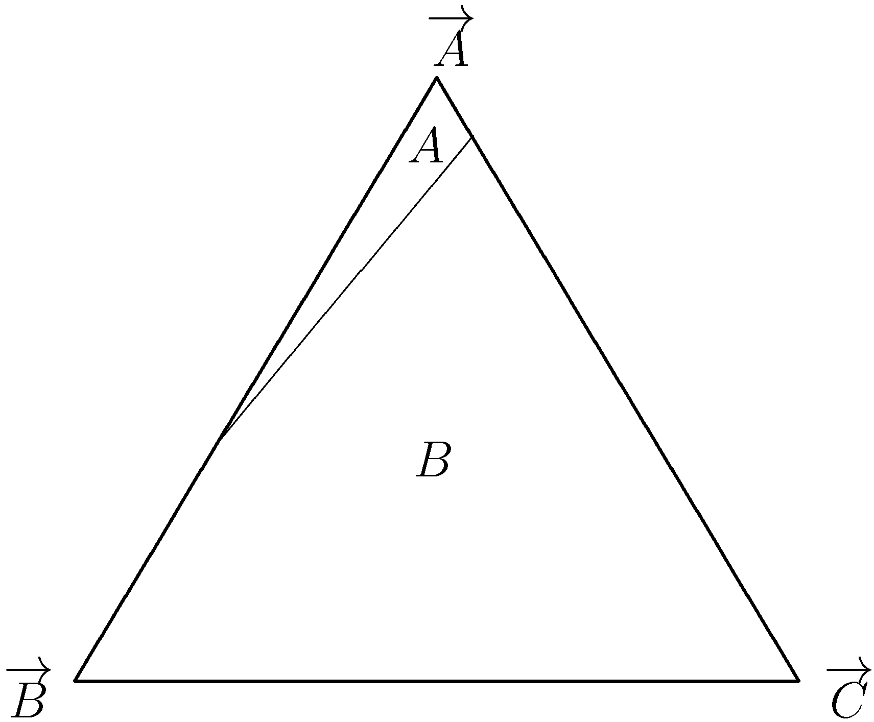
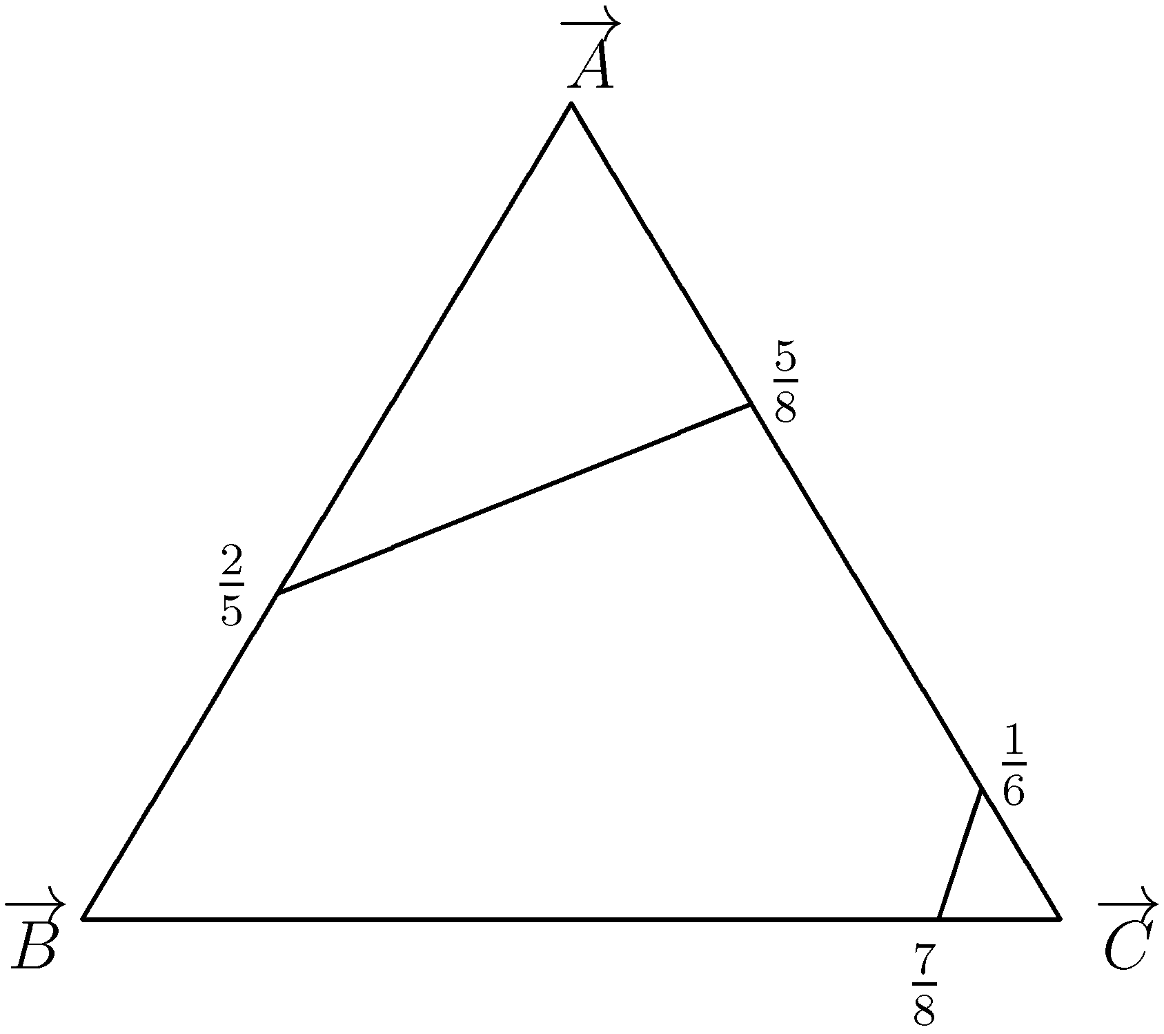
![Games 01 00551 i004]() Note that for strategy C is strictly dominated by both A and B. Furthermore, note that if W is chosen large enough we have that B is a best response whenever only one agent chooses C. Note that this implies that A is no longer -dominant. Figure 1 underscores this point by plotting the best response regions of the extended game. Hence, in the extended game we can move with one mutation from to , implying . For a large enough population, can however not be left with one mutation, establishing . Thus, the global interactions model is not robust to the addition and, hence, deletion, of strictly dominated strategies.
Note that for strategy C is strictly dominated by both A and B. Furthermore, note that if W is chosen large enough we have that B is a best response whenever only one agent chooses C. Note that this implies that A is no longer -dominant. Figure 1 underscores this point by plotting the best response regions of the extended game. Hence, in the extended game we can move with one mutation from to , implying . For a large enough population, can however not be left with one mutation, establishing . Thus, the global interactions model is not robust to the addition and, hence, deletion, of strictly dominated strategies.


Figure 1.
Best response regions of the extended game for large W.

3. Local Interactions
We will now study settings where players only interact with a small subset of the population, such as close friends, neighbors, or colleagues, rather than with the overall population.
3.1. The Circular City
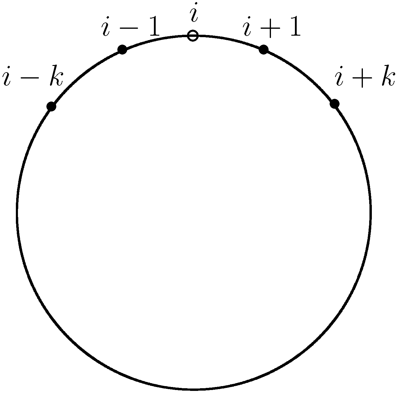
Ellison [9] sets up a local interactions system in the circular city: Imagine our population of N economic agents being arranged around a circle.13 See Figure 2 for an illustration. In this context, one can define as the minimal distance separating players i and j. The shortest way between player i and player j can either be to the left or to the right of player i. Hence, is defined as:
With this specification we can define the following matching rule which matches each player with his k closest neighbors on the left and with his k closest neighbors on the right with equal probability, i.e.,
We assume that , so that no agent is matched with himself and agents are not matched with each other twice. We refer to this setting as the -neighbors model. Of course, it is also possible in this context to think of more sophisticated matching rules such as (for N odd)
This matching rule assigns positive probability to any match. However, the matching probability is declining in the distance separating two players.
Figure 2.
The circular city model of local interaction.

Let us reconsider the -neighbor matching rule. If one given player adopts strategy s against another player who plays strategy , the payoff of the first player is denoted . If is the profile of strategies adopted by players at time t, the average payoff for player i under the -neighbor matching rule is
We assume that each period, every player given revision opportunity switches to a myopic best response, i.e., a player adopts a best response to the distribution of play in the previous period. More formally, at time player i chooses
given the state at t. If a player has several alternative best replies, we assume that he randomly adopts one of them, assigning positive probability to each.
First, let us now reconsider coordination games. Note that we have two natural candidates for LRE, and . Further, note that there might exist cycles where the system fluctuates between different states. For instance, for (and for N even) we have the following cycle
Note, however, that such cycles are never absorbing under our process with positive inertia. For, with positive probability some player will not adjust his strategy at some point in time and the circle will break down.14
Now, note that since strategy A is risk dominant a player will always have A as his best response whenever half of his neighbors play A. Consider k adjacent A-players.
With positive probability the boundary B-players may revise their strategies. As they have k A-neighbors they will switch to A and we reach the state.
Iterating this argument, it follows that A can spread out contagiously until we reach the state . Hence, we have that from any state with k adjacent A-players there is a positive probability path leading to . This implies that .
Second, note that in order to move out of we have to destabilize any A-cluster that is such that A will spread out with certainty. This is the case if we have a cluster of adjacent A-players. For, (i) each of the agents in the cluster has k neighbors choosing A and thus will never switch, and (ii) agents at the boundary of such a cluster will switch to A whenever given revision opportunity. Hence, in order to leave the basin of attraction of we at least need one mutation per each agents, establishing . Hence,
Proposition 4 Ellison [9]. The state where everybody plays the risk dominant strategy is unique LRE under best reply learning in the circular city model of local interactions for .
This is qualitatively the same result as the one obtained for global interaction by KMR. Note, however, that the nature of transition to the risk dominant convention is fundamentally different. In KMR a certain fraction of the population has to mutate to the risk dominant strategy so that all other agents will follow. On the contrary, in the circular city model only a small group mutating to the risk dominant strategy is enough to trigger a contagious spread to the risk dominant convention.
It is an easy exercise to reproduce the corresponding result for the circular city model of local interactions for general games in the presence of a -dominant strategy. Note that we have again, by the definition of -dominance, that a player will have the -dominant strategy as his best response whenever k of his neighbors choose it. Thus, in the presence of a -dominant strategy the insights of the case carry over to general games and we have that,
Proposition 5 Ellison [1]. The state where everybody plays a -dominant strategy is unique LRE under best reply learning in the circular city model of local interactions for .
3.2. On the Robustness of the Local Interactions Model
We will now reconsider the three aforementioned points of critique raised on the model of global interactions within the circular city model of local interactions. The fact that a risk dominant (or - dominant strategy) is contagious under local interactions will turn out to be key in challenging all three points of critique in large population.
First, let us consider the speed of convergence of the local interactions model. As argued already by KMR the low speed of convergence of the global model might render the model’s predictions irrelevant for large populations under global interactions. However, note that under local interactions the speed of convergence is independent of the population size as risk dominant strategies are able to spread out contagiously from a small cluster of the population adopting it. In particular, we have, by Ellison’s [1] Radius-Coradius theorem, that the expected waiting time until is first reached is of order as . This implies that the speed of convergence will be much faster under local interactions as compared to the global model. Therefore, one can expect to observe the limiting behavior of the system at an early stage of play.
Second, reconsider Bergin and Lipman’s [19] critique stating that the prediction of KMR’s model are not robust to the underlying specification of noise. Lee, Szeidl, and Valentinyi [25] argue that if a strategy is contagious the prediction in a local interactions model will be essentially independent of the underlying model of noise for a sufficiently large population. To illustrate their argument let us return to the example of Section 2.4 where agents make mistakes twice as often when they are in the risk dominant convention as in the payoff dominant convention. Note now that the number of mistakes needed to move into the risk dominant convention is still k and, thus, is independent of the population size. To upset the risk dominant convention it now takes mutations (again measured in the rate of the original mistakes). Note, however, that this number of mutations is growing in the population size. Thus, for a sufficiently large population the risk dominant convention is easier to reach than to leave by mistakes and consequently remains LRE.
Weidenholzer [26] shows that the contagious spread of the risk dominant strategy also implies that the local interaction model is robust to the addition and deletion of strictly dominated strategies in large populations. The main idea behind this result is that risk dominant strategies may still spread out contagiously from an initially small subset of the population. Thus, the number of mutations required to move into the basin of attraction of the risk dominant convention is independent of the population size. Conversely, even in the presence of dominated strategies the effect of mutations away from the risk dominant strategy is local and, hence, depends on the population size. To see this point reconsider the extended game from Section 2.4 and consider the circular city model with . Note that it still is true that it takes one mutation to move form to , establishing that . Consider now the extended game and the risk dominant convention . Assume that one agent mutates to C:
With positive probability the C-player does not adjust her strategy whereas the A-players switch to B and we reach the state
Unless, there is no or only one A-agent left, we will for sure move back to the risk dominant convention, establishing that , whenever . Thus, in the circular city model the selection of the risk dominant convention remains for a sufficiently large population.15
One might be tempted to think that the nice features of the local interactions model can be used to justify results of a global interactions model. Note that this is legitimate in the presence of a risk dominant or -dominant strategy which is selected in, both, the global and local framework. In particular, note that in symmetric games there is always a risk dominant strategy. Hence, in games the predictions of the local and the global model always have to be in line. However, once we move beyond the class games the results may differ. To see this point, consider the following example by Young [7].
![Games 01 00551 i005]() Figure 3 depicts the best-response regions for this game. First, note that in pairwise comparisons A risk dominates B and C. Kandori and Rob [11] define this property as global pairwise risk dominance, GPRD. Now, consider the mixed strategy . The best response against σ is B, and hence A is not -dominant. Thus, while -dominance implies GPRD the opposite implication is wrong. The fact that A is GPRD only reveals that A is a better reply than C against σ. Under global interactions, we have that and . Thus, is unique LRE under global interactions in a large enough population.
Figure 3 depicts the best-response regions for this game. First, note that in pairwise comparisons A risk dominates B and C. Kandori and Rob [11] define this property as global pairwise risk dominance, GPRD. Now, consider the mixed strategy . The best response against σ is B, and hence A is not -dominant. Thus, while -dominance implies GPRD the opposite implication is wrong. The fact that A is GPRD only reveals that A is a better reply than C against σ. Under global interactions, we have that and . Thus, is unique LRE under global interactions in a large enough population.

Figure 3.
The best response regions in Young’s example.
Let us now consider the two neighbor model. Consider the monomorphic state and assume that one agent mutates to B. With positive probability we reach the state .
Likewise, consider and assume that one agent mutates to A. With positive probability, we reach the state .
Hence, we have that . Now, consider . If one agent mutates to B he will not prompt any of his neighbors to switch and will switch back himself after some time.
Likewise, assume that one agent mutates to C. While the mutant will prompt other agents to switch to B, after some time there will only be A- and B-players left from which point on A can take over the entire population.
Thus, we can not leave the basin of attraction of with one mutation, implying that . Consequently, is LRE in the two neighbor model, as opposed to in the global interactions framework. Consequently, the nature of interaction influences the prediction.
Furthermore, note that while GPRD does not have any predictive value in the global interactions framework the previous example suggests that it might play a role in the local interactions framework. Indeed, Alós-Ferrer and Weidenholzer [27] show that GPRD strategies are always selected in the circular city model with in games. However, they also show that GPRD looses its predictive power in more general games. Further, they also exhibit an example where non-monomorphic states are selected. Hence, one can also observe the phenomena of coexistence of conventionsin the circular city model of local interactions.16
3.3. Interaction on the Lattice
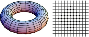
Following Ellison [1], we will now consider a different spatial structure where the players are situated on a grid, rather than a circle.17 Formally, assume that players are situated at the vertices of a lattice on the surface of a torus. Imagine a lattice with vertically and horizontally aligned points being folded to form a torus where the north end is joined with the south end and the west end is joined with the east end of the rectangle. Figure 4 provides an illustration of this interaction structure.
Following [1] one can define the distance separating two players and as
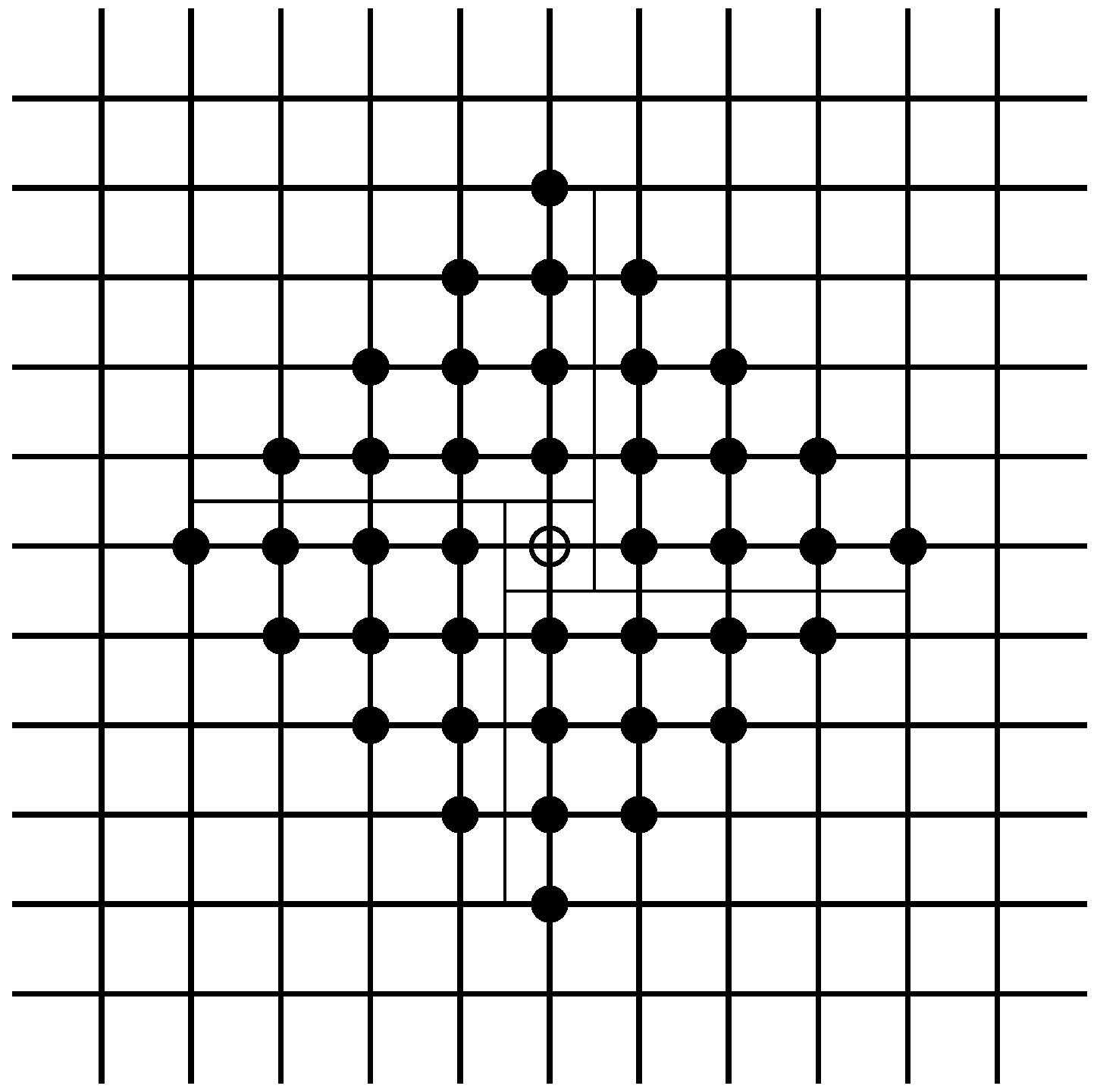
A player is assumed only to be matched with players at a distance of at most k with and , i.e., player is matched with player if and only if . Furthermore, note that (as can be seen from Figure 5) within this setup each player has neighbors. Thus, we define the neighborhood of a player , as the set of all of his neighbors. If ω is the profile of strategies adopted by players at time t, the total payoff for player is
where denotes the strategy of player .
Figure 4.
Interaction on a torus.
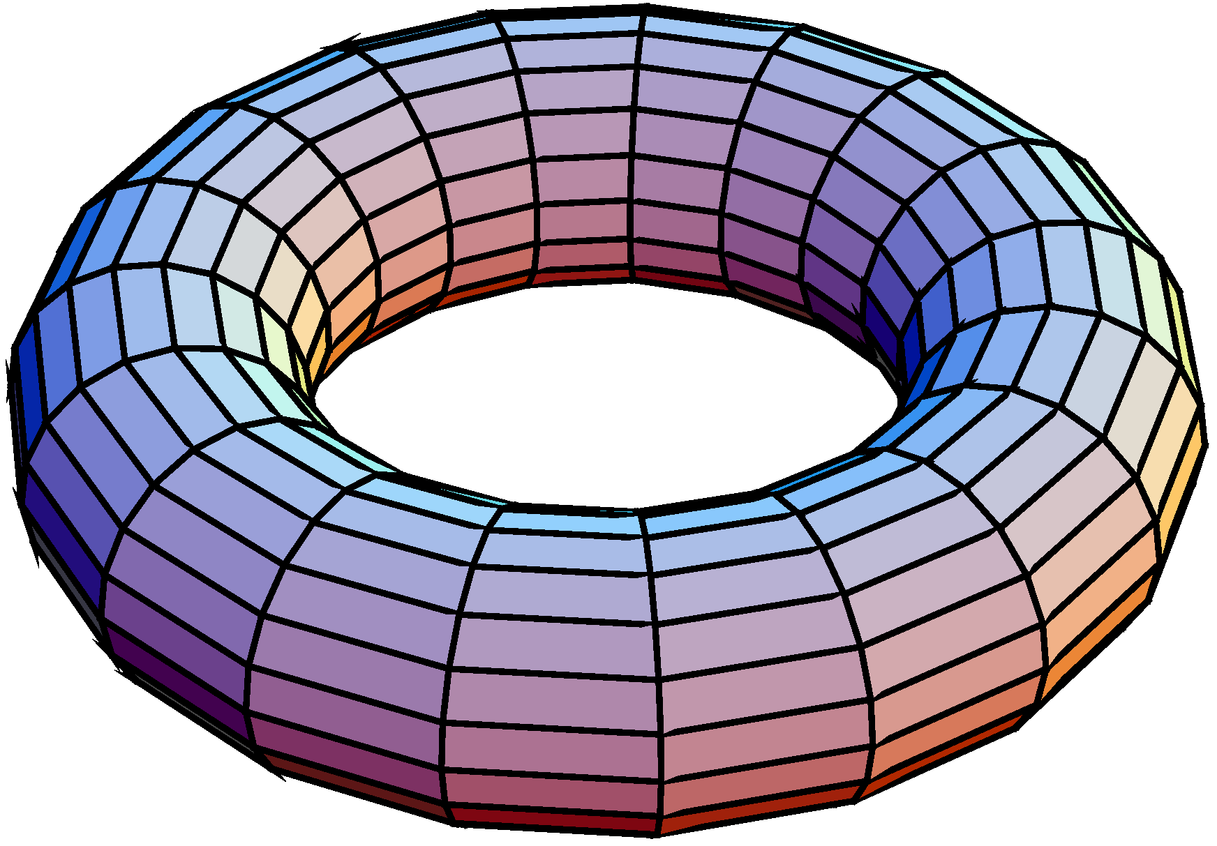
Figure 5.
Neighborhood of size on the lattice. It can be easily seen that a player has neighbors.

Each period, each player might receive the opportunity to revise strategy with positive probability. When presented with a revision opportunity a player switches to a myopic best response. More formally, player at time chooses
given the state at t. Eventual ties are assumed to be broken randomly.
A different kind of adjustment process is the asynchronous best reply process in continuous time used by Blume [21,22]. Each player has an i.i.d. Poisson alarm clock. At randomly chosen moments in time a given player’s alarm clock goes off and a player receives the opportunity to adjust his strategy. Blume [21] considers the following perturbed process. It is assumed that a player adopts a strategy according to the logit choice rule. Under the logit choice rule players choose their strategy according to a full support logit distribution that puts more weight on strategies with a higher myopic payoff. As the noise level decreases the logit choice distribution converges to the degenerate distribution with all mass on the best reply. Blume [21] shows that this process converges to the risk dominant convention in coordination games in the long run. Blume [22] considers an unperturbed adjustment process where whenever given possibility a player always adjusts to a best response to the current distribution of play. In varying the initial conditions he finds that the system converges to the risk dominant convention in coordination games most of the time.
Let us now study Ellison’s [1] model in detail. Assume that each player is only matched with his four closest neighbors with equal probability. Hence, the probability for players and to be matched is given by
Note that, in general there may be many absorbing states. For instance, consider the following game
![Games 01 00551 i006]() If four players in a square configuration play A while the rest of the players plays B the state is absorbing. Each A-player gets a payoff of four. Switching to B would only give him a payoff of two. Hence, the A-players in the square will retain their strategy. Similarly, the adjacent B-players have no incentives to change their strategies since this would decrease their payoff from three to two. One can construct a very large number of such non-monomorphic absorbing states by varying the size, shape, and locus of these blocks of A players.
If four players in a square configuration play A while the rest of the players plays B the state is absorbing. Each A-player gets a payoff of four. Switching to B would only give him a payoff of two. Hence, the A-players in the square will retain their strategy. Similarly, the adjacent B-players have no incentives to change their strategies since this would decrease their payoff from three to two. One can construct a very large number of such non-monomorphic absorbing states by varying the size, shape, and locus of these blocks of A players.

Note that in the two dimensional model a -dominant strategy is not able to spread contagiously as in the one dimensional model. Rather, what matters in the two dimensional model is that clusters of players playing the -dominant strategy grow as players mutating at the edge of these clusters cause new players to join them. Following Ellison [1] we can in fact show that a -dominant strategy (despite not being able to spread contagiously) is unique LRE in the model at hand.
To this end, assume now that strategy A is -dominant. If all players in a cross pattern (e.g., players and players ) play A all of them have at least two neighbors playing A and will retain their strategy. Furthermore, players playing A will expand from the center of the cross until the entire population plays A. So in order to leave we have to destabilize all possible crosses. So we need at least mutations. Hence we have .
Now, consider any state . With at most two mutations we can reach a state where players and play A. There is positive probability that players and retain their strategy and players and also switch to A. We then obtain a square of at least four A-players. Note that since all players in this square have two of their neighbors playing A they will not switch strategies. Furthermore, the dynamics can not destabilize this cluster of A-players. So assume the dynamics shifts us to a new state . If now player mutates to A player will follow. By adding successive single mutations we can shift two rows of players to strategy A. If we now work our way through two columns we obtain a cross configuration from which strategy A is able to spread contagiously. Hence, we can explicitly construct a path of modified cost at most two from to implying . Hence,
Proposition 6 Ellison [1]. A -dominant strategy is unique LRE under best reply learning in the lattice model whenever and .
Furthermore, note that, even though the -dominant strategy is not able to spread contagiously, the speed of convergence is independent of the population size. In particular, we have that the expected waiting time until the risk dominant convention is first reached is of order .
4. Multiple Locations and Network Formation
4.1. Multiple Locations
In the model of Ellison [9] the main reason for the persistence of the risk dominant strategy is its ability to spread contagiously. Whenever an agent has at least half of his neighbors playing the risk dominant strategy playing the payoff dominant strategy is no longer optimal. Ely [31] argues that if the players are free to decide where the game is played an agent playing the risk dominant strategy will prompt his neighbors to move away rather than to change their behavior. Hence, the contagious spread of the risk dominant strategy is no longer possible and societies might achieve efficient outcomes.
Let us now study the basic model of Ely [31] in detail: It is assumed that there are two locations or islands. A population of agents is repeatedly matched within their location to play a symmetric coordination game. Players only interact with players from their location. In particular, players are matched uniformly with the neighbors at their location. So, within a location the matching procedure is uniform whereas if society is considered as a whole matching is local.
Each agent is assumed to receive the average payoff from playing the game against his neighbors.18 Furthermore, it is assumed that a player who is the only player at a location obtains a reservation payoff smaller than either equilibrium payoff. This ensures that players will always prefer an occupied location to an unoccupied one. Each period each agent might receive the possibility to revise his strategy. Whenever this revision possibility arises a player chooses both his strategy in the base game and his location such that they maximize his per-period expected average payoff in the previous period. Ties are broken randomly.19 In addition with probability ϵ an agent makes a mistake and chooses an action and island at random.
Note that this adjustment process converges to a convention where either of the two strategies is played on one location. The reason for this is that as in KMR’s model, all players at one particular location will play the same strategy. In addition, if the payoff dominant strategy is played at some location all players will move to this location. As ties are assumed to be broken randomly the process will at some point settle down at a state where all players reside at the same location. Such a state can never be left without mistakes as no player wants to move to an empty island. So let and denote the set of states where only A, respectively only B, is played on either of the two islands.
Consider first the states where everybody plays the risk dominant strategy A on both locations. If one player mutates, thereby switching to the payoff dominant action B and moving to the empty island, all other players will follow and we reach a state in the set . Further, consider the set of states where all agents on one island play B. In order to move out of the basin of attraction of this set at least a fraction of players has to switch to A.20 Hence, we have that and , which in turn implies:21
Proposition 7 Ely [31]. The states where all players on one location play the payoff dominant strategy are LRE under best reply learning.
So, location and mobility provide players with a tool by which they can identify their preferred opponents and hence achieve efficient outcomes. Similar results have been obtained by Oechssler [29,30]. Oechssler [29] focusses on the initial conditions which favor efficiency in a coordination game. At the beginning of the dynamics each agent randomly chooses a strategy on each location. The initial condition gives rise to a binomial distribution over the distribution of strategies at the different locations. Whenever one location plays the payoff dominant strategy all players will end up playing the payoff dominant strategy. In analyzing these initial condition Oechssler [29] finds that the more locations there are and the less populated these are (i.e., the more decentralized the overall population is) the more likely it is that efficient outcomes will arise. Oechssler [30] builds on the assumption that each strategy of an coordination game is initially played on some location. Further, also interaction between the locations is considered. Bhaskar and Vega-Redondo [49] also exhibit a model where players can choose their preferred location. The focus is on pure coordination games and stag hunt games, though.
4.2. Restricted Mobility
Anwar [32] argues that there may however be constraints limiting the movement of players between locations. In the presence of constraints on mobility not all players can move wherever they want. Some players will be refused at their preferred location and others simply will not want to move. Hence, upsetting inefficient outcomes by just moving away may no longer be possible. Anwar [32] shows that if the constraints on mobility are not too tough the most likely scenario will be the coexistence of conventions.22
Following Anwar [32], let us now introduce constraints on mobility into Ely’s [31] basic model by assuming that the maximum number of agents on a location is with . This might either be due to some agents being immobile or to a constraint on the number of agents allowed on one island.
As in the previous sections, since non-monomorphic configurations at one location are not absorbing, all players at one particular location will play the same strategy. In contrast to Ely [31], it can now be the case that the risk dominant strategy is played on one and the payoff dominant strategy is played on the other location since no more players may be allowed at the efficient location. This implies that we have three classes of absorbing states, one where A is played on one location and B on the other, denoted by , one where both locations play A, denoted by , and one where B is played on both locations, denoted by . Note that in the class the payoff dominant island will always be full up to its capacity. In the classes where either of the two strategies is played at both locations the system will shift between states with a varying number of agents on each island.
To move from to one location has to be shifted to the payoff dominant strategy. As the system will move between states with a varying number of players at each location, the easiest way is by a proportion of mutating to the payoff dominant strategy when only agents are present at one location. To move from to the efficient location (which is full to capacity) has to be shifted to the risk dominant strategy. This requires simultaneous mutations. In order to directly23 move from to a proportion of of the total population has to mutate to the payoff dominant strategy. To move from to only players have to mutate. Now consider . We know that on one location players play A. So in order to move to a fraction of has to mutate to B on this location. To move from to a fraction of players has to mutate to A when .
Now, observe that moving out of (to or ) is possible with mutations, implying . Moving into the basin of attraction of (from or ) takes at most mutations, implying . Hence is LRE for a large enough population whenever
Second, note that if this inequality is reversed we find that states in are LRE for a large enough population since and . Summing up:
Proposition 8 Anwar [32]. Under best reply learning,
- a)
- if the states where the risk dominant strategy is played on both locations are unique LRE.
- b)
- if the states where the risk dominant strategy is played on one location and the payoff dominant strategy is played on the other location are unique LRE.
If the constraints on mobility are sufficiently tough the model approximates KMR’s model on two separate locations and the states where only the risk dominant strategy is played on both locations emerges as long run equilibrium. However, if capacity constraints are rather slack the payoff dominant strategy will be played on one of the two locations. The basic intuition behind this result is the following: Consider the state . First, note that all mobile agents who are allowed will move to location B. The larger the maximum number of agents allowed on an location gets the larger location B gets. However, an increased population on location B implies that more mutations are needed to upset the efficient outcome on this location. Hence, with capacity sufficiently high and/or sufficiently many mobile players the efficient outcome will arise on one of the two locations.
Similar models include Dieckmann [50] and Blume and Temzelides [51]. Dieckmann [50] uses an imitation model to analyze restricted mobility. Furthermore imperfect observability of play outside one’s location is assumed. So players only know with certainty what is going on at their location. In addition the role of friction is analyzed. In this sense players cannot always determine which location to move to. So players use expected payoffs in their reasoning. Dieckmann [50] finds that whereas imperfect observability of play and friction can not prevent efficient conventions, restricted mobility can. Blume and Temzelides [51] also consider a model with heterogeneity in mobility. In studying the payoff differences of mobile and immobile agents Blume and Temzelides [51] find that typically mobile agents obtain higher payoff than immobile ones.
4.3. Network Formation
Note that the assumption, that people move away—thereby breaking up all their relationships and forming new ones—to achieve efficient outcomes is very stringent and is very difficult to justify in real life situation. It might be more plausible to assume that players directly decide with whom to maintain relationships and with whom not.
A recent branch of the literature has studied how social networks evolve as players benefit from the formation of costly links (see e.g., Jackson and Wolinsky [52] or Bala and Goyal [53]). These paper do not consider the choice of actions in a coordination game but rather concentrate on the formation of links. Building on these model of network formation Jackson and Watts [33], Goyal and Vega-Redondo [34], and Hojman and Szeidl [35] present models where players not only choose actions but also choose with whom to establish a (costly) link for interaction.24
We will now present a modified version of Goyal and Vega-Redondo’s [34] model.25 Goyal and Vega-Redondo [34] assume that the interaction structure among a set of individuals is given by a directed graph g. The nodes of this graph are the agents and the links represent interactions between these agents. We denote by a link between players i and j. We write if the link is present in the network and if . Players may only be linked to other player, i.e., for all . We say a link between players i and j is active if and we say a link is passive if . We denote by the case when the network is complete, i.e., all possible links are present ( for all ) and we denote by and the state where everybody is fully connected and plays A and B, respectively.
Players are assumed to play the coordination game G against all players they are (actively and passively) linked with, i.e., against the set of players . We will however assume that players only derive payoff from active links.26 In addition, each player is assumed to pay a cost κ, with , for each active link. So, the payoff received by player i is given by
Note that now agents concentrate on the overall payoff obtained. So, the number of links each player has is crucial here. If one considers average payoff the number of neighbors would not have a strong influence on the behavior of players. In particular, players with the payoff dominant strategy would not have incentives to form links with players using the risk dominant strategy and similarly to Ely’s [31] model this would allow players to achieve efficient outcomes. In Goyal and Vega-Redondo [34] model a player with the payoff dominant action might increase his total payoff by linking to somebody using the risk dominant action.
As before, players are assumed to give a (myopic) best response (i.e., to optimally choose an action and decide on their active links) to the distribution of actions and the link structure present in the previous period. In addition, with small probability ϵ agents make mistakes, thereby choosing links and/or actions different to the one specified by the adjustment process.
In determining the LRE the magnitude of the linking cost will turn out to play an important role. First, consider the case of low linking costs, . In this case, players will always want to link up to all other players, as each link carries a positive payoff regardless of the distribution of actions. Hence the only absorbing states are the two fully connected monomorphic networks and . So, for we essentially obtain global interactions as in KMR and consequently the complete network where everybody plays the risk dominant action A is selected.
In the case of intermediate linking costs, , A-players want to link to all other players, whereas B-players only want to link up to other B-players. This observation will turn out to have a decisive effect when determining the LRE. Let n denote the number of A players present in the population. For given n, an A-player will obtain a payoff of and a B-player who does not link to A-players will obtain a payoff of . Under the myopic best response rule presented in section 2.1 an A-player will switch to B if and only if
Let
then an A-player will switch strategies if and only if . Note that since it always holds that , i.e., if B-players do not link to A-players, then it requires more A-players for A to be a best response as under global interactions. Likewise, one can show that a B-player will switch to A if and only if . Consequently, if an A-player prefers to keep his strategy a B-player will switch and vice-versa, establishing that only the complete monomorphic network architectures and are absorbing.
Now consider the payoff dominant complete network, . In order to move into the basin of attraction of the risk dominant complete network at least players have to mutate to A establishing that . Consider now the risk-dominant complete network, . In order to move into the basin of attraction of the payoff dominant complete network, at least players have to mutate to B. Hence, . For large enough N, the payoff dominant complete network is selected if whereas the risk dominant complete network is selected whenever . Reconsidering reveals that this conditions translate into and , respectively.
In the case of high linking costs, , both, A-players and B-players, only want to link to other players of their own kind. Similar arguments reveal that in this case the payoff dominant complete network is unique LRE. Summing up,
Proposition 9 Goyal and Vega-Redondo [34]. Under best reply learning in a large enough population
- a)
- if the risk dominant complete network is unique LRE,
- b)
- if the payoff dominant complete network is unique LRE.
The main reason behind this result is that if costs are low players obtain a positive payoff from linking to other players irrespective of their strategy. Hence, the complete network will always form and players have no incentive to erase any links. The link formation decision plays an irrelevant role and we are basically back in the framework of KMR where the risk dominant strategy is uniquely selected. If costs of forming links are high the players do not wish to form all links anymore, which gives the payoff dominant strategy a decisive advantage.
Similar models have been presented by Jackson and Watts [33] and Hojman and Szeidl [35]. The setup of Hojman and Szeidl [35] is very similar to the one of Goyal and Vega-Redondo [34]. The focus of this papers however extends to the case when players also benefit from neighbors of neighbors, i.e., from second level partners. The model of Jackson and Watts [33] is different to Goyal and Vega-Redondo [34] in three ways: i) Jackson and Watts [33] assume that the strategy decision and the link formation are independent of each other, ii) in Jackson and Watts [33] the process that governs the formation and deletion of links is based on the (cooperative) concept of pairwise stability in networks (see Jackson and Wolinsky [52]), whereas Goyal and Vega-Redondo [34] use a non–cooperative approach (see Bala and Goyal [53]), and iii) both players involved in a link have to pay its cost. Jackson and Watts [33] show that for low linking costs the risk dominant convention is selected whereas for high linking costs both the efficient convention and the risk dominant conventions are selected. Goyal and Vega-Redondo [34] demonstrate that the fact that Jackson and Watts’ model [33] does not uniquely select the payoff dominant strategy for high linking costs is inherent in the assumption that links and strategies are chosen independently. In particular, the nature of transition from one convention to another is different. In Jackson and Watts [33] this transition is stepwise: starting with a connected component of size two other players mutating will join one-by-one and we gradually reach the other convention, whereas in Goyal and Vega-Redondo’s [34] model, once a sufficiently large number of players plays one strategy all other players will immediately follow.
If, however, one is prepared to identify free mobility with low linking costs, this leaves a puzzle to explain: Ely [31] selects the efficient convention, while Goyal and Vega-Redondo [34] select the risk dominant one. It seems that the main reason for this discrepancy lies in the fact that Ely [31] considers average payoffs whereas Goyal and Vega-Redondo [34] consider additive payoffs. This implies that in Ely’s [31] model the number of potential opponents does not matter and players will always prefer to interact with a small number of players choosing the payoff dominant strategy than with a large number choosing the inefficient strategy. On the contrary, in the framework of Goyal and Vega-Redondo [34] the additive payoff function implies that all links will form, giving rise to the risk dominant convention.27
Staudigl and Weidenholzer [56] exploit a similar idea by considering a model where agents may only maintain a limited number of links, with the motivation being that in many situations the set of interaction partner of a given agent is small compared to the overall population. Under these premises agents will have to carefully decide on whom to establish one of their precious links to. Thus, under constrained interactions agents face a tradeoff between the links they have and those they would rather have, creating a fairly strong force allowing agents to reach efficient outcomes. Staudigl and Weidenholzer [56] provide a full characterization of the set of long run outcomes under constrained interactions. Whereas payoff dominant networks will be selected if the number of allowed links is low and/or linking cost are high, risk dominant network configurations are only selected if the number of allowed links is high and linking costs are low.
5. Imitation
Note that in many situations economic agents lack the computing capacity to give a best response. Further, information costs might constrain them in gathering or processing all the information necessary to play a best response. Within a different context, it has to be noted that games are simplified representations of reality: it might be the case that the players who play the game do not recognize that they are actually playing a game, are not aware of the exact payoff structure, or simply do not know what strategies are available. In addition to this, people usually tend to be able to have a good estimate of how much their neighbors earn or what social status or prestige they enjoy. Under these circumstances players might be prompted to just copy successful behavior and abandon strategies that are less successful, thereby giving rise to an adjustment rule based on imitation, rather than rules based on best response.28
As already mentioned beforehand, the classic model of KMR is of an imitative nature. Within their setting agents imitate the strategy that has earned the on average highest payoff in the previous period. The underlying assumption in their adaptive process is that in each round all possible pairs are formed and agents concentrate on the average payoffs of these pairs. As in the case of best reply learning KMR’s imitative process leads to the adoption of the risk dominant convention in the long run. Robson and Vega-Redondo [12] consider a modification of KMR’s framework where agents are randomly matched in each round to play the coordination game and imitate strategies that earn high payoffs. Surprisingly, this process leads to the adoption of the payoff dominant strategy in the long run. The main reason behind this result is that once there are two agents playing the payoff dominant strategy they will be matched with strictly positive probability and may achieve the highest possible payoff. Under imitation learning all player will from then onwards adopt the payoff dominant strategy.
In order to best convey the underlying idea behind Robson and Vega-Redondo’s [12] model, we will work with the Imitate the Best Max Rule, IBM, which prescribes players to imitate the strategy that has yielded the highest payoff to some player. In Robson and Vega-Redondo [12] original model players imitate strategies that have on average yielded the highest payoff, giving rise to the Imitate the Best Average Rule, IBA.29 The basic insights and the qualitative results are very similar under the two imitation rules, with the advantage of IBM being that it allows for a quicker and clearer exposition of those. Further, note that there is also a conceptual drawback of the IBA rule: If a strategy earns different payoffs to different players it can be the case that the player with the highest payoff switches strategies. To see this point, suppose there are three players. Further, suppose that players 1 and 2 use strategy s and earn a payoff of 1 and 0, respectively and player 3 uses strategy and earns a mediocre payoff of . In this case, player 1 would switch strategies, even though he earns the highest payoff. Obviously, under the IBM rule it can never be the case that a player abandons the most successful strategy.30
Let us now consider the model of Robson and Vega-Redondo [12] in more detail. Consider a population of N players, where N is assumed to be even. In each round the population is randomly matched into pairs to play our coordination game. Any way of pairing these players is assumed to be equally likely. Note that three different kinds of pairs can be formed: a pair of two A-players with a payoff of a to both of them, a pair of two B-players with a payoff of b to both of them, and a mixed pair with an A- and a B-player with a payoff of c to the former and a payoff of d to the latter player.
In each round, an agent presented with the opportunity to revise his strategy is assumed to copy the agent that has earned the highest payoff in the previous rounds. As above, with probability ϵ the agent ignores the prescription of the adjustment rule and chooses a strategy at random.
First, note that under the IBM rule only the two monomorphic states and are absorbing. To see this point, assume that some agent i earns the highest payoff in the overall population. With positive probability all agents may revise their strategy and will adopt the strategy of agent i. Thus, with positive probability we will reach either of the two monomorphic states. Now, consider the risk dominant convention and assume that two agents mutate to B. With positive probability, these two agents will be matched and will earn the highest possible payoff of b. With positive probability, all agents receive revision opportunity and will switch to B. Thus, there exists a positive probability path leading to the payoff dominant convention. It follows that we have, . Now, consider the payoff dominant convention . In order to move out of the basin of attraction of we need to reach a state that is such that no pair forms. For, otherwise all revising agents would adopt B. Thus, we need at least mutations to B, implying . It follows that,
Proposition 10 Robson and Vega-Redondo [12]. The state where everybody plays the risk dominant strategy is unique LRE under the IBM rule and under random matching for .
Thus, the combination of imitation and a random interaction framework yields selection of the payoff dominant convention. This is remarkable in the sense that KMR select the risk dominant convention if interaction takes the form of a round robin tournament and points into the direction that imitation together with an “appropriate” interaction structure might allow agents to coordinate on the efficient convention.
We will now explore this idea in more detail within the local interactions framework of Ellison [9]. It will turn out to be useful to normalize the payoff structure of the underlying game. Following Eshel, Samuelson, and Shaked [13], without loss of generality one can transform payoffs to obtain
![Games 01 00551 i007]() where and . Note that for coordination games we have and . Further, payoff dominance of translates into and risk dominance of now reads as .
where and . Note that for coordination games we have and . Further, payoff dominance of translates into and risk dominance of now reads as .

Alós-Ferrer and Weidenholzer [14] consider a setting where agents use the IBM rule to update their strategies. They find that whether a risk dominant or a payoff dominant convention will be established in the long run depends on the interaction radius of the individual agents. Formally, define the interaction neighborhood (modulo N) of a player i, as the set of all of his neighbors. Thus, if is the profile of strategies adopted by players at time t, the total payoff for player i is
Assume that each player observes the strategies played and the payoffs received by himself and all his neighbors. When given revision opportunity, an agent is assumed to adopt the strategy that has earned the highest payoff in his interaction neighborhood in the previous period.
Alós-Ferrer and Weidenholzer [14] find that when players only interact with their two closest neighbors the selection of the risk dominant strategy persists. The logic behind this result is the following: One can show that there is a large number of absorbing states, where clusters of A- and B-players alternate, and that these states can be connected to each other through chains of single mutations.
Let us consider this point in more detail. In order to shorten our exposition, we only consider the case where holds and remark that if similar results can be obtained. So, consider the efficient convention and assume that two players mutates to A.
The B-players next to the A players earn a payoff of 1, all B players further away earn a payoff of 2, and the inner A-players earn a payoff of . Thus, under the IBM rule none of these players will switch and, thus, this state is absorbing. Now, we can reach by a chain of single mutations. Hence, we have .
Conversely, consider the risk dominant convention and assume that two agents mutate to B.
Now the B-players earn a payoff of 1, whereas the inner and the outer A-players earn a payoff of and , respectively. Hence, none of the A-players will switch and the B-players will revert to A. Thus, two mutations are not enough to leave the risk dominant convention, establishing . It follows that,
Proposition 11 Alós-Ferrer and Weidenholzer [14]. In the two neighbor circular city model the risk dominant strategy is the unique LRE under the IBM rule.
However, for larger neighborhoods payoff dominant strategies might be LRE. To see this point, consider the -neighbors model and consider a state with adjacent A-players.
The two middle B-players earn a payoff of . The boundary A-players obtain a payoff of at most provided that . The boundary A-players observe the payoff of the middle B-players and hence will switch strategy if .
In the next period, at least four middle B-players earn . Iterating this argument, we reach the efficient convention .
This implies that for any state with adjacent B players lies in the basin of attraction of .31 Note that we can move into with mutations implying . To move out of the basin of attraction of , we need to eliminate all B-clusters of size . This requires at least one mutation per cluster, i.e., . holds for . Hence,
Proposition 12 Alós-Ferrer and Weidenholzer [14]. In the -neighbor circular city model a payoff dominant strategy is the unique LRE under the IBM rule for in a sufficiently large population.
This implies that efficient conventions are easier to establish in larger neighborhoods. Furthermore, for every coordination game there exists a threshold neighborhood size such that an efficient equilibrium is LRE.
Alós-Ferrer and Weidenholzer [15] consider a more generalized framework which applies to arbitrary networks. They show that if the information available (slightly) extends beyond the interaction neighborhood players coordinate on payoff dominant equilibria. The idea behind these “information spillovers” is that agents who interact with each other routinely also exchange information on what is going on in their respective interaction neighborhoods.32 We will now lay out the main ideas of Alós-Ferrer and Weidenholzer [15] model within the -neighbors model of Ellison [9].
Alós-Ferrer and Weidenholzer [15] make a clear distinction between the interaction neighborhood and the information neighborhood. Players play the game against players in their interaction neighborhood but receive information about the pattern of play from their information neighborhood. As above, the interaction neighborhood of player i is given by (modulo N). The information neighborhood of player i is assumed to consist of himself and his , with nearest neighbors. i.e., (modulo N). Players are assumed to always know what is going on in their interaction neighborhood, i.e., . When deciding about their future behavior players consider the pattern of play in their information neighborhood. According to the IBM rule, a player adopts a strategy that has earned the highest payoff in his information neighborhood in the previous period. So, when revising strategies players do not only consider what is happening within their interaction neighborhood but also take into account the relative success of players who are not direct opponents.
Assume now that players always receive information from beyond their interaction neighborhood. So and . The most important feature of this setup is that once payoff dominant outcomes are established somewhere they can spread contagiously. This is similar to the spread of risk-dominant strategies in Ellison’s [9] best-reply local interaction model.
The main reason for this result is that any state with adjacent B-players lies in the basin of attraction of . To see this, consider any state with adjacent B-players. In the worst case they are surrounded by A-players.
The inner B-player now earns a payoff of , which is the highest possible payoff. All B- players and the boundary A-players up to a distance of m from the inner B-player observe that A earns this maximum payoff. Hence, the B-players will retain their strategy and the boundary A-players will switch to B. In a next step the “new" boundary players will also change to A and so forth. In this manner B will extend to the whole population and we will eventually reach the state . Thus, three mutations to B are sufficient for a transition from to . Furthermore, from any hypothetical non-monomorphic state in an absorbing set, also mutations suffice for a transition to . Hence, we have .
By the observation above, in order to leave the basin of attraction of we at least have to destabilize every B-cluster of size three. Hence, we need at least mutations, implying that . For , holds and we have that,
Proposition 13 Alós-Ferrer and Weidenholzer [15]. In the -circular city model with information neighborhood the payoff dominant convention is the unique LRE under the IBM rule in a sufficiently large population.
In fact, Alós-Ferrer and Weidenholzer [15] provide an even more general result which also applies to non-regular networks:33 Whenever information extends beyond the interaction neighborhood,34 the payoff dominant convention is unique LRE, provided that the number of disjoint neighborhoods of a network exceeds the number of players in the smallest neighborhood. The intuition behind this result is that once the efficient convention is played at some neighborhood (the smallest included) it will spread to the entire population. On the contrary, to upset the efficient convention it has to be destabilized in every disjoint neighborhood.
6. Conclusions
Roughly speaking, one can summarize the main insights of this survey in the following way: If the interaction structure is fixed and players use myopic best rules risk dominant conventions will arise in the long run in a large variety of models. In addition, in the presence of a contagious strategy local interactions models seem to be robust to a number of critiques mentioned in the literature on global interactions. Further, we have seen that if agents may in addition to their strategy choice either move between multiple location or decide on whom to form a costly link to the message arising is not so clear. Depending on the exact specifications of the model, we might either observe efficient outcomes, risk dominant outcomes, or the coexistence of conventions. Furthermore, if agents learn by imitation we might observe efficient outcomes in the long run in “appropriate” interaction structures.
Although coordination games have been extensively studied in learning models the economic applications of these results have been somewhat neglected. A notable exception is, e.g., presented by Kandori and Rob [11] who briefly discuss the interplay between efficiency, compatibility, and equilibrium selection in a global interactions model. Another fruitful application is provided by Möbius [63] who uses an evolutionary local interactions model to study the rise and fall of local service competition in the US telephone market at the beginning of the 20th century.35 There seems, however, to be a much potential in studying the implications of boundedly rational agents choosing among different technology standards on competition between rational firms.36 For instance, consider the mobile telecommunication industry, where firms typically set higher prices for call terminating on a different network than for call terminating on the same network. This pricing policy clearly gives rise to coordination games. Further, the calling pattern of customers is typically of a local type: Customers are more likely to call somebody they know than calling anybody chosen randomly out of the telephone book.37 In this sense, one could set up a model where firms maximize their (long run expected) profits given the (long run) behavior of a set of boundedly rational agents. This setup would allow for an alternative discussion of the implications of issues such as regulation or access pricing in this industry. In this light there seems to be much potential for future research applying the theoretical findings to deliver new economic insights on topics such as competition policy or the survival of inefficient technology standards.
Acknowledgements
I thank Carlos Alós-Ferrer, Matthew O. Jackson, Manfred Nermuth, Nick Netzer, and an anonymous referee for helpful comments and suggestions. Financial support from the Austrian Science Fund (FWF) under project fund P18141-G09 and from the Vienna Science and Technology Fund (WWTF) under project fund MA 09-017 is gratefully acknowledged.
References
- Ellison, G. Basins of Attraction, Long-Run Stochastic Stability, and the Speed of Step-by-Step Evolution. Rev. Econ. Stud. 2000, 67, 17–45. [Google Scholar] [CrossRef]
- Jackson, M.O. The Economics of Social Networks. In Proceedings of the 9th World Congress of the Econometric Society, London, UK, 19–24 August 2010; Blundell, R., Newey, W., Perrson, T., Eds.; Cambridge University Press: Cambridge, UK, 2005; pp. 1–56. [Google Scholar]
- Goyal, S. Connections: An Introduction to the Economics of Networks; Princeton University Press: Princton, NJ, USA, 2007. [Google Scholar]
- Vega-Redondo, F. Complex Social Networks; Econometric Society Monograph Series; Cambridge University Press: Cambridge, UK, 2007. [Google Scholar]
- Foster, D.P.; Young, P. Stochastic Evolutionary Game Dynamics. Theor. Pop. Biol. 1990, 38, 219–232. [Google Scholar] [CrossRef]
- Kandori, M.; Mailath, G.J.; Rob, R. Learning, Mutation, and Long Run Equilibria in Games. Econometrica 1993, 61, 29–56. [Google Scholar] [CrossRef]
- Young, P. The Evolution of Conventions. Econometrica 1993, 61, 57–84. [Google Scholar] [CrossRef]
- Sobel, J. Economists’ Models of Learning. J. Econ. Theory 2000, 94, 241–261. [Google Scholar] [CrossRef]
- Ellison, G. Learning, Local Interaction, and Coordination. Econometrica 1993, 61, 1047–1071. [Google Scholar] [CrossRef]
- Kandori, M.; Rob, R. Evolution of Equilibria in the Long Run: A General Theory and Applications. J. Econ. Theory 1995, 65, 383–414. [Google Scholar] [CrossRef]
- Kandori, M.; Rob, R. Bandwagon Effects and Long Run Technology Choice. Game. Econ. Behav. 1998, 22, 30–60. [Google Scholar]
- Robson, A.J.; Vega-Redondo, F. Efficient Equilibrium Selection in Evolutionary Games with Random Matching. J. Econ. Theory 1996, 70, 65–92. [Google Scholar] [CrossRef]
- Eshel, I.; Samuelson, L.; Shaked, A. Altruists, Egoists, and Hooligans in a Local Interaction Model. Amer. Econ. Rev. 1998, 88, 157–179. [Google Scholar]
- Alós-Ferrer, C.; Weidenholzer, S. Imitation, Local Interactions, and Efficiency. Econ. Lett. 2006, 93, 163–168. [Google Scholar] [CrossRef]
- Alós-Ferrer, C.; Weidenholzer, S. Contagion and Efficiency. J. Econ. Theory 2008, 143, 251–274. [Google Scholar] [CrossRef]
- Freidlin, M.; Wentzell, A. Random Perturbations of Dynamical Systems, 2nd ed.; Springer Verlag: New York, NY, USA, 1988. [Google Scholar]
- Harsanyi, J.; Selten, R. A General Theory of Equilibrium Selection in Games; The MIT Press: Cambridge, MA, USA, 1988. [Google Scholar]
- Morris, S.; Rob, R.; Shin, H. p-dominance and Belief Potential. Econometrica 1995, 63, 145–157. [Google Scholar] [CrossRef]
- Bergin, J.; Lipman, B.L. Evolution with State-Dependent Mutations. Econometrica 1996, 64, 943–956. [Google Scholar] [CrossRef]
- Kim, C.; Wong, K. Long-run equilibria with dominated strategies. Game. Econ. Behav. 2010, 68, 242–254. [Google Scholar] [CrossRef]
- Blume, L. The Statistical Mechanics of Strategic Interaction. Game. Econ. Behav. 1993, 5, 387–424. [Google Scholar] [CrossRef]
- Blume, L. The Statistical Mechanics of Best-Response Strategy Revision. Game. Econ. Behav. 1995, 11, 111–145. [Google Scholar] [CrossRef]
- Alós-Ferrer, C.; Netzer, N. The logit-response dynamics. Game. Econ. Behav. 2010, 68, 413–427. [Google Scholar] [CrossRef]
- Myatt, D.P.; Wallace, C. A Multinomial Probit Model of Stochastic Evolution. J. Econ. Theory 2003, 113, 286–301. [Google Scholar] [CrossRef]
- Lee, I.H.; Szeidl, A.; Valentinyi, A. Contagion and State Dependent Mutations. B.E. J. Theor. Econ. 2003, advances.3. [Google Scholar]
- Weidenholzer, S. Long-Run Equilibria, Dominated Strategies, and Local Interactions; Mimeo; University of Vienna: Vienna, Austria, 2010. [Google Scholar]
- Alós-Ferrer, C.; Weidenholzer, S. Partial Bandwagon Effects and Local Interactions. Game. Econ. Behav. 2007, 61, 1–19. [Google Scholar] [CrossRef]
- Durieu, J.; Solal, P. Adaptive Play with Spatial Sampling. Game. Econ. Behav. 2003, 43, 189–195. [Google Scholar] [CrossRef]
- Oechssler, J. Decentralization and the Coordination Problem. J. Econ. Behav. Organ. 1997, 32, 119–135. [Google Scholar] [CrossRef]
- Oechssler, J. Competition among Conventions. Math. Comput. Organ. Theory 1999, 5, 31–44. [Google Scholar] [CrossRef]
- Ely, J.C. Local Conventions. Adv. Theor. Econ. 2002, 2, 1–30. [Google Scholar] [CrossRef]
- Anwar, A.W. On the Co-existence of Conventions. J. Econ. Theory 2002, 107, 145–155. [Google Scholar] [CrossRef]
- Jackson, M.O.; Watts, A. On the formation of Interaction Networks in Social Coordination Games. Game. Econ. Behav. 2002, 41, 265–291. [Google Scholar] [CrossRef]
- Goyal, S.; Vega-Redondo, F. Network Formation and Social Coordination. Game. Econ. Behav. 2005, 50, 178–207. [Google Scholar] [CrossRef]
- Hojman, D.; Szeidl, A. Endogenous Networks, Social Games, and Evolution. Game. Econ. Behav. 2006, 55, 112–130. [Google Scholar] [CrossRef]
- Alós-Ferrer, C.; Schlag, K. Imitation and learning. In The Handbook of Rational and Social Choice; Anand, P., Pattanaik, P., Puppe, C., Eds.; Oxford University Press: Oxford, UK, 2009. [Google Scholar]
- Sandholm, W.H. Simple and Clever Decision Rules for a Model of Evolution. Econ. Lett. 1998, 61, 165–170. [Google Scholar] [CrossRef]
- Vega-Redondo, F. Game Theory and Economic Applications; Cambridge University Press: Cambridge, UK, 2003. [Google Scholar]
- Karlin, S.; Taylor, H.M. A First Course in Stochastic Processes, 2nd ed.; Academic Press: San Diego, CA, USA, 1975. [Google Scholar]
- Kajii, A.; Morris, S. The Robustness of Equilibria to Incomplete Information. Econometrica 1997, 65, 1283–1309. [Google Scholar] [CrossRef]
- Maruta, T. On the Relationship between Risk-Dominance and Stochastic Stability. Game. Econ. Behav. 1997, 19, 221–234. [Google Scholar] [CrossRef]
- Fudenberg, D.; Levine, D. The Theory of Learning in Games; The MIT Press: Cambridge, MA, USA, 1998. [Google Scholar]
- Arthur, W.B. Competing Technologies and Economic Prediction. Options 1984, 2, 1–3. [Google Scholar]
- Schelling, T. Dynamic Models of Segregation. J. Math. Sociol. 1972, 1, 143–186. [Google Scholar] [CrossRef]
- Young, P. Individual Strategy and Social Structure; Princeton University Press: Princeton, NJ, USA, 1998. [Google Scholar]
- Möbius, M.M. The Formation of Ghettos as a Local Interaction Phenomenon. Mimeo; Harvard University: Cambridge, MA, USA, 2000. [Google Scholar]
- Anderlini, L.; Ianni, A. Path Dependence and Learning from Neighbors. Game. Econ. Behav. 1996, 13, 141–177. [Google Scholar] [CrossRef]
- Morris, S. Contagion. Rev. Econ. Stud. 2000, 67, 57–78. [Google Scholar] [CrossRef]
- Bhaskar, V.; Vega-Redondo, F. Migration and the Evolution of Conventions. J. Econ. Behav. Organ. 2004, 13, 397–418. [Google Scholar] [CrossRef]
- Dieckmann, T. The Evolution of Conventions with Mobile Players. J. Econ. Behav. Organ. 1999, 38, 93–111. [Google Scholar] [CrossRef]
- Blume, A.; Temzelides, T. On the Geography of Conventions. Econ. Theory 2003, 22, 863–873. [Google Scholar] [CrossRef]
- Jackson, M.O.; Wolinsky, A. A Strategic Model of Social and Economic Networks. J. Econ. Theory 1996, 71, 44–74. [Google Scholar] [CrossRef]
- Bala, V.; Goyal, S. A Noncooperative Model of Network Formation. Econometrica 2000, 68, 1181–1229. [Google Scholar] [CrossRef]
- Staudigl, M. Potential Games in Volatile Environments. Game. Econ. Behav. 2010. (Forthcoming. [Google Scholar]
- Tomassini, M.; Pestelacci, E. Coordination Games on Dynamical Networks. Games 2010, 1, 242–261. [Google Scholar] [CrossRef] [Green Version]
- Staudigl, M.; Weidenholzer, S. Constrained Interactions and Social Coordination; Mimeo; University of Vienna: Vienna, Austria, 2010. [Google Scholar]
- Apesteguía, J.; Huck, S.; Oechssler, J. Imitation—Theory and Experimental Evidence. J. Econ. Theory 2007, 136, 217–235. [Google Scholar] [CrossRef] [Green Version]
- Barron, G.; Erev, I. Small Feedback-Based Decisions and their Limited Correspondence to Description-Based Decisions. J. Behav. Decis. Making 2003, 16, 215–233. [Google Scholar] [CrossRef]
- Erev, I.; Barron, G. On Adaptation, Maximization, and Reinforcement Learning among Cognitive Strategies. Psychol. Rev. 2005, 112, 912–931. [Google Scholar] [CrossRef] [PubMed]
- Alós-Ferrer, C.; Weidenholzer, S. Imitation and the Role of Information in Overcoming Coordination Failures; Mimeo; University of Vienna: Vienna, Austria, 2010. [Google Scholar]
- Lieberman, E.; Novak, M.; Hauert, C. Evolutionary Dynamics on Graphs. Nature 2005, 433, 312–316. [Google Scholar] [CrossRef] [PubMed]
- Berninghaus, S.; Haller, H. Local Interaction on Random Graphs. Games 2010, 1, 262–285. [Google Scholar] [CrossRef] [Green Version]
- Möbius, M.M. Death through Success: The Rise and Fall of Local Service Competition at the Turn of the Century; Mimeo; Harvard University: Cambridge, MA, USA, 2001. [Google Scholar]
- Alós-Ferrer, C.; Kirchsteiger, G.; Walzl, M. On the Evolution of Market Institutions: The Platform Design Paradox. Econ. J. 2010, 120, 215–243. [Google Scholar] [CrossRef]
- Laffont, J.J.; Rey, P.; Tirole, J. Network Competition: II. Price Discrimination. RAND J. Econ. 1998, 29, 38–56. [Google Scholar] [CrossRef]
- 1.Of course, the articles presented in this survey just reflect a selection of the literature within this field.
- 2.See Sobel [8] for a review of various learning theories used in models of bounded rationality.
- 3.A notable exception are adjustment dynamics that give rise to a Birth-Death process.
- 4.See also Blume [21,22] for local interaction models where agents are arranged on grid structures. The dynamics in these models are based on the logit-response dynamics and, thus, do not allow for an application of the mutation counting techniques used in this paper. Note, however, that Alós-Ferrer and Netzer [23] provide an analogous of Ellison’s Radius-Coradius Theorem for the logit-response dynamics. Further, see Myatt and Wallace [24] for a global interactions model where payoffs, rather than actions, are subject to normally distributed idiosyncratic noise. It turns out that the resulting best response process is characterized by the logit form and that the long run equilibria can be found using the Freidlin and Wentzell approach. This suggest that a properly adopted version of Ellison’s Radius-Coradius Theorem might also be used in their model.
- 5.See Alós-Ferrer and Schlag [36] for a detailed survey on imitation learning.
- 7.i.e., we present a model with positive inertia and we will stick to this specification in the subsequent exposition. This modelling choice has the advantage of keeping most of the analysis as simple as possible, while at the same time not changing the results of the models discussed in this exposition.
- 8.We remark that the results are qualitatively the same, though.
- 9.Ellison [1] gives the nice example of the evolution from a mouse into a bat. Assume that this transition takes two mutations. After one mutation the mouse grows a flap of skin and after one further mutation evolves into a bat. If the creature with the flap may survive the transition between a mouse and a bat occurs much faster than if the creature with was not viable.
- 10.Where in the following we denote by the smallest integer larger than x and by the largest integer smaller than x.
- 11.More generally, for any , a strategy s is called p-dominant if s is the unique best response against any mixed strategy σ such that . Kajii and Morris [40] change this definition dropping the uniqueness requirement.
- 12.This process is closely related to the concept of fictitious play, see e.g., Fudenberg and Levine [42].
- 13.The basic framework is due to Schelling [44] who uses a circular city model to analyze the process of neighborhood segregation. An evolutionary analysis of this model is provided by Young [45]. See also Möbius [46] for an evolutionary model of neighborhood segregation allowing for a richer (local) interaction structure. This richer setup can explain some historical empirical regularities associated with neighborhood segregation.
- 14.In the absence of inertia these cycles would form absorbing sets. However, they can be destabilized very easily by only one mutation. Durieu and Solal [28] introduce spatial sampling in Ellison’s [9] model of local interactions. Under spatial sampling players observe a random fraction of the pattern of play in their neighborhood. The addition of this element of randomness also turns out to be sufficient to rule out cycles in the absence of inertia.
- 15.Note that the bound on the population size is larger in the extended game than in the original game. Weidenholzer [26] exploits this observation to show that for small population sizes one can reverse also the predictions of the -neighbors model.
- 16.See section 4.2 for a multiple locations model where coexistence of conventions can also occur.
- 18.Note that in the models discussed so far it was irrelevant whether one considers average payoffs or the sum of payoffs. However, if considering multiple locations with a varying number of inhabitants this difference is crucial.
- 19.Ely [31] assumes that agents who are indifferent agents stay put. For the sake of exposition, we choose to work with tie breaking. Without tie breaking all monomorphic states where there are no loners are absorbing. Tie breaking avoids those states. The prediction for LRE and the basic logic behind the result are the same, though.
- 20.Recall that is the set of states where all agents live at one location and play B. If we consider only one of these states one mutation is sufficient to move out of its basin of attraction, thereby moving into the state where B is played on the other location.
- 21.In fact, Ellison’s [1] Radius-Coradius Theorem here only tells us that the LRE is contained in . However, appealing to the fact that both states in this set can be reached from each other with one mutation shows that both of them have to be LRE.
- 22.Coexistence of conventions is actually a very widespread phenomenon. For example, in some areas of the world people have agreed to drive on the left hand side of the road whereas in other areas people chose to drive on the right side.
- 23.In fact, the indirect transition via would be cheaper.
- 25.We choose to present the model of Goyal and Vega-Redondo [34] in more detail as it best fits in the previously presented framework.
- 26.In the main model discussed by Goyal and Vega-Redondo [34] players also derive payoff from passive links. For the sake of exposition, we discuss a version of the model where passive links do not matter, remarking that our results are qualitatively similar. Goyal and Vega-Redondo [34] also briefly discuss the implications of such a model in their extensions section.
- 27.Ely [31] also considers a variation with an additive payoff structure. He shows that there exists a parameter region such that the risk dominant strategy is selected.
- 29.Eshel, Samuelson, and Shaked [13] study players located on a circle playing a prisoners’ dilemma game against their closest neighbors. They find that under the IBA rule agents will overcome the prisoners’ dilemma and achieve cooperative outcomes in the long run.
- 30.Further, Barron and Erev [58] and Erev and Barron [59] find in a large number of decision making experiments that highest recent payoffs are particulary attractive to decision makers, even if they are associated with a low expected return. This suggests that the IBM rule might be more realistic description of reality than the IBA rule.
- 31.Note that in the two neighbor model this inequality reads and, thus, can never hold in the presence of a risk dominant strategy.
- 32.See also Alós-Ferrer and Weidenholzer [60] for an analysis of efficiency in minimum-effort network games in the presence and in the absence of information spillovers.
- 33.See Morris [48] for model of general networks with an infinite population based on best reply, see Lieberman, Novak, and Hauert [61] for a network model of evolutionary game theory based on a Moran process, and see Berninghaus and Haller [62] for a model where the local interaction structure exogenously changes over time.
- 34.For instance, if players observe their neighbors’ neighbors.
- 35.The model argues that while local service competitors where initially successful over time consumers’ desire to communicate with customers from other (unconnected) networks increased which, in turn, led to the downfall of local competitors and the re-monopolization of the market by the initial monopolist AT&T.
- 36.See e.g., Alós-Ferrer, Kirchsteiger, and Walzl [64] studying competition between rational market designers when confronted with boundedly rational agents who learn which market platform to select.
- 37.A uniform calling pattern is predominantly assumed in the industrial organization literature on mobile telecommunication, see e.g., Laffont, Rey, and Tirole [65].
© 2010 by the author; licensee MDPI, Switzerland. This article is an open access article distributed under the terms and conditions of the Creative Commons Attribution license ( http://creativecommons.org/licenses/by/3.0/).
Share and Cite
MDPI and ACS Style
Weidenholzer, S. Coordination Games and Local Interactions: A Survey of the Game Theoretic Literature. Games 2010, 1, 551-585. https://doi.org/10.3390/g1040551
AMA Style
Weidenholzer S. Coordination Games and Local Interactions: A Survey of the Game Theoretic Literature. Games. 2010; 1(4):551-585. https://doi.org/10.3390/g1040551
Chicago/Turabian StyleWeidenholzer, Simon. 2010. "Coordination Games and Local Interactions: A Survey of the Game Theoretic Literature" Games 1, no. 4: 551-585. https://doi.org/10.3390/g1040551