Application of Machine Learning Models in Error and Variant Detection in High-Variation Genomics Datasets †


1
Faculty of Mathematics and Informatics, Sofia University, 5 James Bourchier Blvd., 1164 Sofia, Bulgaria
2
Institute of Mathematics and Informatics, Bulgarian Academy of Sciences, Acad. Georgi Bonchev Str., Bl. 8, 1113 Sofia, Bulgaria
*
Author to whom correspondence should be addressed.
†
This paper is an extended version of the paper “Machine learning models in error and variant detection in high-variation high-throughput sequencing datasets” presented at the International Conference on Computational Science ICCS 2017 (Zürich, Switzerland, 12–14 June 2017) and published in Procedia Computer Science, Vol. 108 (2017).
Computers 2017, 6(4), 29; https://doi.org/10.3390/computers6040029
Submission received: 7 October 2017
/
Revised: 5 November 2017
/
Accepted: 7 November 2017
/
Published: 10 November 2017
(This article belongs to the Special Issue Biomedical and Bioinformatics Challenges for Computer Science)
Abstract
:For metagenomics datasets, datasets of complex polyploid genomes, and other high-variation genomics datasets, there are difficulties with the analysis, error detection and variant calling, stemming from the challenges of discerning sequencing errors from biological variation. Confirming base candidates with high frequency of occurrence is no longer a reliable measure because of the natural variation and the presence of rare bases. The paper discusses an approach to the application of machine learning models to classify bases into erroneous and rare variations after preselecting potential error candidates with a weighted frequency measure, which aims to focus on unexpected variations by using the inter-sequence pairwise similarity. Different similarity measures are used to account for different types of datasets. Four machine learning models are implemented and tested.
1. Introduction
A lot of genomics research has to deal with high-variation datasets. This includes metagenomics [1], where it is common to work with the genomes of multiple organisms in the same sample, and polyploid species [2] that have more than one similar and hard-to-differentiate subgenomes.
Metagenomics studies microorganism communities in environmental samples. These range from soil samples in agriculture [3] to human microbiome in health research [4]. Whether these studies have a specific focus on the individual variations, or a general focus on the diversity and interspecies evolutionary relations, they all face difficulties because of the errors in the datasets [5], which has led to a common practice of discarding entire sequences suspected to contain errors [6]. For error correction to be applicable in those fields, errors in the experimental reading need to be correctly distinguished from the natural sources of variation, such as single-point polymorphisms (SNPs), which account for genuine differences between biological organisms, and are the target of research whose preservation is necessary.
With the development of relatively cheap and fast sequencing methods, this approach is becoming excessively prohibitive and unsuitable. New research efforts have focused on mapping the microbiome of urban environments across the world [7], requiring the sequencing and analysis of a vast amount of samples, collected in various urban environments. These are increasingly relying on nanopore sequencing, whose speed and price had come at the expense of quality—nanopore error rates average 5–8% [8], with some studies measuring errors of up to 40% [9]. This necessitates the use of precise error detection and correction approaches, as the assurance of quality has to be moved from the hardware platform to the software post-processing stage.
Problems of similar nature are encountered by the researchers who analyse polyploid genomes. An example in this regard is the hexaploid bread wheat, or common wheat. It has six sets of chromosomes inherited from three distinct species that diverged between ~5–6 and 7 million years ago, and merged again in two hybridisation events that happened between 2300–4300 and 5800–8200 years ago [2]. As a result, any computational research has to process and analyse three copies of the genome, which in divergent genes and loci may be easy to differentiate, but in conserved loci may be only identifiable by subtle differences, which are hard to discern from the occasional errors. In contrast to metagenomics samples, where there might be anywhere from hundreds to millions of individual biological organisms, each carrying their own individual variation, polyploid samples come from the same organism, possessing several multiple subgenomes, comprising the different sources of genetic code and variation.
The complex and unstudied nature of the discussed types of datasets makes them a suitable target for the application of machine learning (ML) approaches, which allows the creation of models that incorporate properties that are not yet explored, or difficult to formalise.
2. Methodology of Error Detection
This paper introduces a methodology aimed at discerning natural variations from errors of the sequencing procedure. This methodology is based on a combination of two types of methods for data analysis. The first method is used to select the suitable error candidates and may be characterized as an analytical one. It applies similarity weights between the pairs of sequences to find the bases which are rare among fuzzy groupings of close sequences. The selected candidates are then filtered with a classification model that is based on an appropriate ML method, and rests on frequency vectors.
For the analytical approach, a weighted frequency function is introduced, and it is used together with a pairwise similarity function. Given a particular base in a particular sequence read, this weighted frequency helps to answer the question: which bases are infrequent in the fuzzy set of sequences that are similar to the evaluated one? Two accompanying similarity functions are proposed and tested for metagenomics, and another one—for hexaploid wheat.
The similarity weights alone are not enough to precisely isolate the errors, which is why the candidates need to be filtered using a ML-based classification model. Artificial neural networks (ANN) [10] were initially chosen as the primary model, because they can be trained to produce a numerical value proportional to the error probability, instead of a simple binary classification, and that could allow one to use these results inside a more complex fuzzy error model.
In addition, a random forest (RF) [11], a Hoeffding tree (HT) [12], and Repeated Incremental Pruning to Produce Error Reduction (RIPPER) propositional rule learner [13] have been implemented and tested in two separate computational experiments.
Experimental Data and Preprocessing
Several input datasets were used to evaluate the presented methods. Each dataset contains sequences of genomic reads, which are sequences over a four-letter alphabet (A, C, G and T), called bases, and correspond to the four nucleotide bases of DNA. The sequences in each evaluated dataset contain the same region of the genome of a large number of different microorganisms. Because of the interspecies differences and the amount of sampled organisms, the reads in the dataset have a high degree of variation, and this is a major obstacle for performing error discovery.
Before preprocessing, the datasets contained between 30,000 and 50,000 sequences of up to 1000 bases. After the preprocessing, the datasets contained sequences with lengths between 300 and 500 bases, and were clustered in sets of up to 6000 sequences. The larger of those clusters were selected for testing, as the smallest ones did not provide high enough coverage for analysis.
3. Analytical Selection of Error Candidates
The essence of the proposed basic approach to picking error candidates is to select bases by their frequency, using their similarity as a weight. The following weighted frequency function was introduced in [14].
It computes the weighted frequency of the base rk at position k in read r, among all reads in the dataset R. It focuses on the reads similar to r using the similarity function sim(r,p,k). Error candidates—bases rare among those reads—are selected by comparing (1) to a threshold.
Using similarity weights when computing the frequencies, we would focus the evaluation of bases on the similar reads. Thus, the frequency of each evaluated base would be computed in an implicit fuzzy set of reads similar to its read in the region surrounding it. This would reduce the effect of variation by excluding locally dissimilar reads from the first stage of the base evaluation. In this manner, we do not flag bases solely based on large dissimilarity within a region. However, the fuzzy grouping alone would not be sufficient to identify errors without the ML-based model in the second stage of the evaluation.
3.1. Similarity Weights for Metagenomics
For the processing of metagenomics data, consisting of medium-long reads (300–500 bases) of the same region, it seemed prudent to compute the similarity on the bases close to the evaluated position k. This would minimise the effect of problems in other parts of the sequences and, in particular, the effect of the especially inaccurate tails present in the test datasets. During the empirical selection of the parameters for the ML-based models in Section 4.2, it was discovered that distant bases had little effect on the classification accuracy (see R3 in Section 5.1.5). For these reasons, a window with radius w around the evaluated position was selected.
window(r, k) = {i: ∃ri, i ∈ [k − w, k − 1] ∪ [k + 1, k + w]}
To reduce the effect of the sudden cutoff at the window edges, and to reduce the importance of w as a parameter, the similarity functions include a fading factor q, which decreases the importance of differences further from the evaluated base. The fading factor is an empirically evaluated parameter with different specifics in the different proposed weight functions, however as it only accounts for the initial error candidate selection, the effect of its fine tuning is diminished once the candidates are filtered with the ML-based models. Two similarity measures were tested.
The first similarity corresponds to the commonly used Hamming distance [15].
However, it results in an additive penalization of differences, meaning that each additional difference linearly reduces the similarity with the same fixed amount. In reality, differences occurring by chance (i.e., errors) are independent and unlikely, hence it makes sense to use a multiplicative penalization instead—that way, each difference would significantly increase the chance that the pair of sequences have different origins.
For this reason, the following “sharp” similarity was also tested, with the expectation that its interpretation of differences would be closer to their biological meaning.
It should be noted that while the sharp similarity indeed proved to be a better selector for error candidates, once the ML-based filter was applied afterwards, the difference was no longer visible in the final results. For this reason, little focus has been put on the choice of similarity function and its parameters. However, removing the similarity weight altogether leads to a measurably worse error selection even after the ML-based filter, demonstrating its importance.
Accounting for pairwise similarity alone would not give a large enough difference with the amount of variation in a dataset. To further improve the separation between the errors and the genuine variation, the expected error rates of the sequencing machines were taken into account. A dataset with known bases was repeatedly sequenced, and the amount of errors at given positions was measured. The resulting measurement was repeated, until an error rate could be computed. To reduce noise in the error rates in regions with fewer errors, a Gaussian blur filter was applied to the vector of error rates.
The threshold for errors was chosen to be a linear function of the error rate using an empirically chosen multiplier. This more precise threshold would sacrifice less of the genuine variations in regions with lower error rates, while still providing a good trade-off at regions with high variation.
3.2. Similarity Weights for Polyploid Genome Sequencing Data Analysis
For the processing of hexaploid wheat data, a significantly modified similarity function was needed. The sequence reads were much shorter, and would contain various fragments from different locations inside the wheat genome. Most significantly, pairs of sequences would have various degree of overlap, ranging from 1 to 50–60 bases. This means that limiting the evaluation inside a window would be less beneficial, while it would be necessary to take the sequence overlap into account. For these reasons, the following similarity measure was used instead.
In addition to the similarity formula, a different technique for the choice of the error candidate threshold was used. For metagenomics, a simple variable per-position threshold, proportional to the measured local error rate, was computed. In contrast, the position-agnostic threshold used in polyploid processing had to take into account the predicted distribution of the three subgenomes in the sample. It also had to be adjusted to match the type of base variant errors had to be distinguished from.
For that reason, a more complex model, published in [16], modelling the subgenome distribution and computing the threshold, was used during candidate selection.
3.3. Computing the Distribution and Threshold for Polyploid Genomes
To account for the nature of the data samples, a more complex model, published in [16], modelling the subgenome distribution and computing a sample- and read-tailored threshold, was used during candidate selection.
Samples from allohexaploid wheat contain similar but different reads from multiple subgenomes that, during its past evolution, diverged from a single genome. During error filtering, not only should the error score be focused on the similar reads from the same subgenome as with metagenomics, but the threshold itself can be selected in accordance to distribution of reads from the different subgenomes in the sample. In particular, proper threshold selection is required for solving the problem of finding heterozygous [17] SNP—single-base mutations that would naturally only be present in one of the two alleles, or in other words, in roughly half the reads of that subgenome. The thresholds for such SNPs, including the lower error threshold, need to be a function of the percentage of reads belonging to that subgenome.
This should be a straightforward choice. Unfortunately, not all reads can be computationally attached to a subgenome, creating a problem that is twofold: the actual subgenome distribution is not really known, and not all reads can be attached to a single—or any—subgenome. As a result, the subgenome distribution needs to be approximated, and a non-exact determination needs to be made for ambiguous reads.
In [16], we determined that there is more than one way to approximate the distribution, by making different assumptions about the distribution of the subgenomes among ambiguous reads, compared to their distribution among all reads. The direct results from these different approaches were not consistent. However, even without an expectation that bases from ambiguous reads can be classified with complete accuracy, extended testing demonstrated that the choice of approximation did not greatly affect the final result of either the SNP calling and error filtering. The difference additionally decreased when the additional ML filtering was applied later.
Using an estimate for subgenome distribution in a sample, together with a prediction for the subgenome which a read belongs to, the computation of lower and upper thresholds for a heterozygous SNP (a mutation present in half of the reads of a subgenome) is straightforward. If signifies the portion of reads predicted to belong to subgenome i, the upper thresholds for SNPs and errors in such reads were set as follows:
For reads ambiguously mapped to more than one subgenome, the average of the two or three values was used. In reads with no predicted subgenome affiliation, that meant that bases with frequency between 13.3% and 20% were predicted to be heterozygous SNPs, which would be the same as if all subgenomes comprised exactly a third of the sample.
Four different schemes for the subgenome proportions were used:
- “All even”. All subgenomes are assumed to occupy a third of a sample. That was used as a control.
- Simple proportions. All reads predicted to belong to a subgenome were counted for their predicted subgenome. The counts of reads predicted to belong to one of two subgenomes were distributed evenly among them—half for one of those subgenomes, and half for the other. Unknown reads that could not be mapped to any subgenomes were distributed evenly among all three:
- One-step proportions. Like in simple proportions, unambiguous reads were counted for their respective subgenome. Any reads with ambiguity were not evenly distributed among the counts, but were distributed in proportion to the counts of the unambiguous reads:
- Two-step proportions. The distribution of unambiguous reads was used to determine the distribution of counts of reads ambiguous between two subgenomes. Then, the predicted distribution of those two was used to distribute the counts of reads not associated with any subgenomes.
3.4. Applying the Rates and Thresholds for Error Detection and SNP Calling
The rates computed using (1) provided a good separation between errors and valid bases, or a good enough starting point before this separation was further refined using the ML-based filter. They are compatible with both the variable thresholds proportional to the error rate for metagenomics, and the complex per-read threshold computed for wheat. Errors occur randomly in the data, so their coincidence with other variation reduces the probability for an error, which was used to justify their use. This coincidence would be relevant in error detection regardless of the rationale and choice for threshold.
However, this makes the similarity-based frequency unsuitable for selection of SNP variants. On one hand, real variation does coincide with other instances of real variation, and the use of focusing on similar regions would only produce an unwanted bias. On the other hand, with a complex model for computing the subgenome ratios—thus the expected thresholds for SNPs—skewing the rates with any form of focusing can put them outside of the chosen range for SNPs. That is acceptable when one is trying to separate the potential SNPs from the errors, but not when bases are selected as a specific type of variation (SNP or otherwise) among a large set of conforming bases.
Thus, for error calling in metagenomics and polyploid genomes, the frequency (1) would be used. But for SNP selection in wheat, it would be replaced by a standard frequency, with sim(r, p, k) = 1.
4. Machine Learning Approach
The main task is to distinguish errors, which occur by chance, from natural variants, which have a complex unknown relationship with the remaining bases. Because variants would be reproduced in other sequences, the use of frequencies seems reasonable, but it is insufficient.
Machine learning provides the tool to create models of complex unknown relationships, which makes them very suitable for the final classification of the error candidates produced in Section 3. Using a single training scheme, we trained four different ML-based classification models. Unlike the selection of error candidates, the same machine learning models were used for both metagenomics and polyploid genomes. These models can either further reclassify the error candidates pre-selected using (1) in Section 3, or can be applied to all bases.
4.1. Machine Learning Models
The ML-based classification models were selected among those offered by the Weka machine learning suite [18]. Twenty different models were tested for raw accuracy on the training sets, without preselection of error candidates using the analytical approach from Section 3, and then four of them were picked for the full testing and tested in two separate experiments on metagenomics.
Artificial neural networks [10] are inspired by the biological neural network comprising the brain. They consist of several layers of “neurons”—numerical values computed using a non-linear parametric formula from the previous layer of neurons. The parameters are changed until the model produces a prediction with an optimal accuracy. They can model complex non-linear dependencies, and can produce non-discrete outputs.
Their application was motivated by the ANN features that make them particularly suitable for this work. This primarily includes their ability to be trained to recognise more complex relationships between the input and output values, as exist in genomic data. Additionally, the ANN models can make predictions in real number values, as opposed to classification into categories or finite integer values. This allows us to use the ANN predictions inside a previously developed Fuzzy Logic model for combining multiple predictions [19].
Random forests [11] rely on a set of decision trees trained by a random selection of features. The prediction uses the statistical mode of all the predictions from the individual trees. They are very fast predictors commonly used for a wide variety of tasks in bioinformatics.
The RF models were selected based on their initial raw performance in a three-way split of the training data, as well as two independent sets of training data [20]. In this test, among the 20 different models, random forests produced the highest accuracy, with only 0.05–0.08% correct bases misclassified as errors—the most critical factor in our choice, given the abundance of correct bases, compared to the small number of errors.
However, as is discussed in the results section, they ended up performing poorly with preselection.
Hoeffding trees [12] are built using a very fast decision tree (VFDT) model. It produces trees similar to the trees produced by the C4.5 algorithm, but it relies on a Hoeffding bound [21] limiting the amount of attributes for making a decision. It uses a smaller sample of the data to select the splitting attribute, applying a statistical measure that estimates the reduced number of observations which is required to compute the splitting attribute. For that reason, it can be trained faster, and can be further refined should new examples be provided.
While incremental learning is not of particular importance for the task of discovering errors, the ability to produce the models quickly may be highly useful because of the way custom models are constructed for each individual dataset. In addition, Hoeffding trees had a very high raw accuracy without preselection of error candidates alongside C4.5 trees, and they also had comparable performance to ANNs with preselection.
RIPPER [13] is a propositional rule learner. Its name stands for Repeated Incremental Pruning to Produce Error Reduction. It is based on the Incremental Reduced Error Pruning (IREP) algorithm, which uses a grow-and-simplify approach. The training data is split into two. Two-thirds of the training examples are used as a growing set, and a collection of propositional rule overfitting it is constructed. The remaining one third of the training examples is used to prune the rules overfitting the growing set, until the rules attain high accuracy on the pruning set. The resulting set of rules is used as a classification model.
RIPPER was one of the best performing models in the direct evaluation using the data from the training sets. It misidentified only 0.06% correct bases as errors in the test on an independent set of training data, and was second after RF among the tested models. It was outperformed by C4.5 decision trees in a three-way split of the same training set, but the performance on an independent set was considered more significant, and RIPPER was chosen. In the final evaluation, like RF, it performed poorly with preselection.
A naïve Bayes classifier [22] is a probabilistic classifier that attempts to estimate the probability of an outcome, given the incidence of a set of features whose absolute and conditional probabilities are known. Under the naïve assumption that these features are independent, the probability of the different outcomes can be computed using the product of the feature’s probabilities. If the logarithm of the product is used, the model becomes a linear model.
Support vector machines (SVM) [23] are non-probabilistic linear models that place training examples in a high-dimensional space, and compute the hyperplanes providing a separation of examples into categories with the largest possible margin. To account for non-linear relations that cannot be separated by a hyperplane, the lower dimensional space is mapped into a higher dimensional space using kernel functions chosen for simple computation. With a well-chosen mapping, in the higher dimensional space, the examples can now be linearly separable.
The last two linear models were tested during the error filtering on wheat.
4.2. Learning Input
The ML-based models would classify an input example for a given evaluated base rk—preselected by (1) or otherwise—producing a Boolean prediction (correct or incorrect) as its output. Each example in our models would be a vector of frequency statistics about the base rk. In particular, each number would be its frequency in a different subset of the reads.
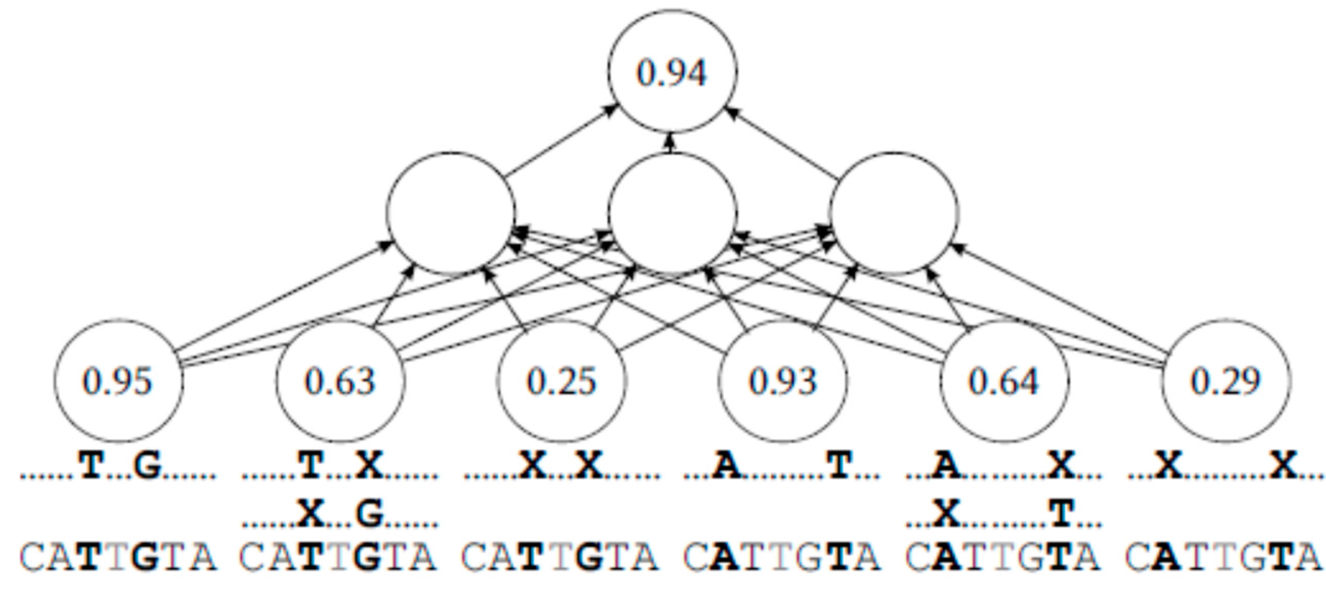
For several pairs of adjacent bases (at a given offset k ± i), the set of remaining reads R\{r} would be split into three subsets—the reads p that match in both of those positions (rk ± i = pk ± i), the reads p that match in only one of those positions (rk − i = pk − i or rk + i = pk + i), and the reads p that match in neither of the two (rk ± i ≠ pk ± i). For each of those subsets, a number would be added to the input vector signifying the frequency of base rk at position k among the chosen subset of R\{r}. This is illustrated on Figure 1.
With this scheme, the first input number would be the portion of reads that contain the evaluated middle base, and that also coincide in the two adjacent bases. The second input number would be the portion of reads containing the middle base that coincide only with the adjacent base on the right, or with the adjacent base on the left, but not both. The third input number would be the portion of reads containing the evaluated middle base that coincide in neither of the adjacent bases. This is repeated with reads split on more distant pairs of bases.
4.3. Training with Virtual Errors
Except in the nanopore datasets, the error rates are very low. This was true in both the metagenomics and polyploid sequencing datasets that were processed as part of our evaluation. The actual errors in the datasets would provide insufficient number of training examples for the ML-based models. Additionally, researchers might want to retrain the models for the kind of data and equipment that they use, in the absence of known errors. For these reasons, the ML-based models were trained using so-called virtual errors.
Because of the low error rate, an average base in the reads can be assumed with high probability to be correct, and can be used as a negative training example, classified as a correct base. Each such example can be supplanted by a second, positive example, classified as an error, in which that particular base has been replaced with one of the other three bases (a virtual error). There’s less than 1% chance that these training examples would be themselves incorrect [24], and they would only slightly affect the classification accuracy of the model.
Thus, for each base, two training examples are produced. The first example contains the vector from Section 4.2, classified as correct. For the second example, which is classified as an error, the same vector is computed after substituting the correct base with a random incorrect one. In this manner, the models are trained to recognise incorrectly substituted bases appearing in any position.
On high-quality sequencing technologies such as 454, the number of wrong training examples using this technique will be low. Using the whole sequences, the wrong training will be up to 1%—the mean error rate for the whole sequences. However, since the sequences have been trimmed to 500 bases, and their noisy ends [24] have been removed, the wrong training examples will be significantly less than 1%. When technologies with high error rate, such as Oxford Nanopore, are used, additional provisions would need to be made to reduce the effect of errors on the ML-based model classification accuracy and bias.
5. Experiments and Results
A comprehensive set of experiments were performed to validate the proposed error detection methods. This includes empirical evaluation of all the parameters of the ML-based model, the parameters of the ANN model in particular, the evaluation of different similarity measures in the analytical approach, and others. Only the important results are summarised in this section.
5.1. Experiments on Metagenomics Sequencing Data
The metagenomics test dataset includes two sets of data containing between 30,000 and 50,000 short reads of up to 1000 bases, produced by the 454 platform from environmental samples from copper mines. To reduce length biases, reads shorter than 300 bases were excluded from the test, and reads longer than 500 bases were trimmed. This is motivated by the sudden increase in errors seen after 500 bases, and in order to maintain sequences of consistent lengths for the experiment. The sets were clustered with CD-HIT-454 [25], generating sets of up to 6000 sequences, and the largest were used for the test.
In addition to the metagenomics dataset, a set of known sequences was available to measure the exact error rate produced by the sequencing machine, which was used in the validation procedure to simulate errors with the same distribution.
5.1.1. Validation
Like finding a good training set, it is difficult to obtain a good testing set. For this reason, the full test, with preselection of candidates, relies on a two-phase validation procedure previously published in [14]. In the first phase, the number of error predictions is measured on the original dataset, which is then corrected with bases picked using the analytical approach. In the second phase, simulated errors are introduced in the data, and the number of missed errors is measured.
The second phase directly measures the sensitivity on simulated errors, and the first phase indirectly indicates the specificity of the error classification algorithm through the overall number of error predictions. A probabilistic method was applied to measure the distribution of errors produced by the sequencing machine used in the metagenomics experiment, so the simulated errors follow the same pattern.
The aim is to get the highest projected specificity (or lowest number of predictions) in phase one, without affecting the sensitivity in phase two, or without affecting it a lot. This is of significant importance, because the errors represent a disproportionally small part of the data, and any over-sensitivity would produce a significant amount of false positives.
5.1.2. Using the Similarity-Based Analytical Approach
The first experimental comparison involved measuring the effect on specificity after introducing the weighted frequency (1). As shown in Table 1, by using the similarity weights alone, the selection of error candidates is reduced by 6–35% without any consistent decrease in the number of missed errors when the similarity measure is added to the frequency formula.
5.1.3. Using ML-Based Filtering
Initially, the training data from Section 4.3 was split into training and test set to measure the raw model accuracy, without preselection of error candidates. Most of the ML models had a raw accuracy over 99%. The ANN model had a sensitivity of 99.563%, and a specificity of 99.705%. The RF model had a sensitivity of 99.760%, and a specificity of 99.922%. The RIPPER model had a sensitivity of 99.714%, and a specificity of 99.748%.
It was not enough to compare the accuracy without preselection, as the achieved specificity was insufficient for the small observed error rates. Furthermore, an interaction may exist between the preselection and the filter. For that reason, the combination of the ML-based filter on candidates selected by the weighted frequency (1) was compared to the naïve predictions using regular frequencies, applying the procedure from Section 5.1.1. This is shown on Table 2.
As can be seen, both the ANN and RF algorithms, when combined with the similarity weights, lead to a major increase in the specificity, throwing out 47.3–61.4% of rare bases that are not errors. The ANN model does that without any drop in the sensitivity—in fact, because of the weights, there are more correctly identified simulated errors.
Unfortunately, here the RF model shows a significant increase in the number of missed errors. Even though it had a very high sensitivity when selecting among all bases, that sensitivity is significantly diminished when applied to only the bases preselected by the analytical approach. This is the kind of interaction between the preselection and filter that necessitates testing the two methods together, and not individually. For that reason, RF was excluded from further testing.
5.1.4. Filtering Accuracy of ANN, RIPPER and HT
The final comparison on metagenomics data aims to highlight only the effect of the ML-based model, when it is applied on the error candidates preselected by the analytical approach, thus measuring the ML-based contribution to the combination. This allows us to compare the ML-based models, and their performance with preselection, without having to think about the performance of the preselection itself.
As seen in Table 3, HT and ANN have a comparable specificity, each outperforming the other on a different test dataset. The ANN seems to show the more significant over-performance of the two, which seems to indicate it as the better method, pending further testing.
RIPPER outperforms both methods in specificity, but its sensitivity on missed errors among the preselected candidates, similarly to RF, is incredibly low. On one of the two datasets, RIPPER filtered only half of the simulated errors, which is insufficient.
HT shows the highest sensitivity, but more tests are needed to demonstrate this with statistical significance.
Both HT and ANN appear to be highly suitable in detecting errors among candidates selected using weighted frequencies, while RF, HT and RIPPER raw results show promise they may be suited to detect errors without initial candidate pre-selection. This discrepancy may be explained with lower result independence between the selection by the analytical approach with weighted frequencies, and the RIPPER and RF models. If ANN and HT use more complex features unused by the frequency formulas that may be the reason for the better results when requiring confirmation from both of those methods.
5.1.5. Results during Model Parameter Tuning
In addition to the main results above, several other test results need to be mentioned.
- R1.
- Before the ML-based filter, using a non-uniform threshold reduces the number of corrections with 5.59–151.91%, without a consistent increase in the number of missed simulated errors.
- R2.
- Before the ML-based filter, using the “sharp” similarity function (4) instead of (3) reduces the number of corrections with 3.765–11.916%, without a consistent increase in the number of missed simulated errors. When measured with a ML filter, the difference in the number of corrections is less than 1%, and the result is inconsistent.
- R3.
- Varying the ML input vector size on a test without error candidate preselection shows that there is no increase in the accuracy beyond an offset of six positions, with the 12 nearest bases being enough. Using only distant bases leads to significantly worse accuracy. Using 12 bases at an offset more than four gives worse accuracy than using only the four nearest bases.
- R4.
- Adding a ML input with the position in the read leads to no change in the accuracy.
5.2. Application during Variant Calling in Complex Polyploid Genomes
In polyploid sequencing datasets, the difficulty in detecting the errors is less significant, as there are only three subgenomes, versus potentially hundreds of different organism species and a larger number of individuals. This may make it easier for the proposed combination to identify the errors, which is why we performed a few computational experiments on polyploid wheat datasets. Unfortunately, due to the lack of a dataset to measure the error distribution with, we could only measure the raw training accuracy of the ML-based models on the data from Section 4.3, and we could not employ the same validation as in metagenomics. In addition, it was not possible to validate the results from either the analytical approach, or fully validate the final results of the ML-based hybrid approach, but only to compare them and draw more generic conclusions, prior to their eventual full validation.
Table 4 shows the results of the application of the analytical approach that was specially adapted to hexaploid genomes, and wheat in particular. It compares the number of predicted SNPs and errors with the three different approaches for computing the subgenome distribution. They are put alongside the “all even” control and a naïve approach that completely disregards the existence of subgenomes. It’s seen that the result is significantly affected by taking the subgenome ratios into account, while at the same time the difference between the different approaches to approximate the ratio is not that significant. In particular, the more complex one-step and two-step proportions yield almost no discernible difference.
The expectation is that the difference between the approaches to compute the subgenome ratio would mostly affect bases that are either in reads whose subgenome could not be determined, or are very close to the threshold. In either of those cases, the accuracy of the result could not be expected. Hence the bases that account for the difference in Table 4 are expected to be bases for which no definitive SNP determination can be made, and the result for which will be further refined with the ML-based filtering.
Table 5 shows the ANN raw accuracy, without preselection of candidates using the analytical approach. The above-99% accuracy seen in Section 5.1.3 seems to still hold in wheat. Another interesting feature is the complete lack of missed errors. It should be also noted that the misidentified correct bases are close to the suspected error rate of the sequencing equipment. Because of the nature of the procedure for generating the training and raw testing dataset in Section 4.3, the error rate may need to be subtracted from the rate of misclassified correct bases. The result is therefore consistent with a hypothesis that the ML-based model alone, without any preselection, offers a high-enough accuracy for error detection in wheat. This, however, cannot be confirmed without performing more rigorous validation, similar to the one in Section 5.1.1.
The good prediction accuracy is also preserved when different ML-based methods are used, as shown in Table 6. Random forest models had the highest possible accuracy, only slightly outperforming neural networks, and the use of SVM with a linear kernel had raw accuracy approaching that of ANNs. The Naïve Bayes classifier performed worse than all the other tested methods. It should be noted that all tested methods, with the exception of Naïve Bayes, retained almost all of the artificially introduced errors, as was already observed for ANN. This signals that these models are a good way to filter error predictions without discarding real errors, with the ANN and RF models being good candidates for standalone use.
To judge the effect of the error detection on variant calling results, the analytical approach from Section 3, using the similarity function (5), and the set of threshold formulas published in [13], was used to preselect errors, as well as select SNP variants using their frequency. Then the preselected errors were filtered using the ANN model. The ANN model confirmed 98.49–99.85% of the predicted SNPs, reclassifying the rest as errors, and confirmed only 12.1–23.26% of the predicted errors, reclassifying the rest as potential SNPs. This is shown in Table 7.
The validity of these choices would need to be confirmed by a more rigorous validation procedure, but as evidenced, the ML-based model significantly impacts the selection of variants.
6. Conclusions
This paper presents a combination of two approaches to identify errors in high-variation datasets, such as found in metagenomics and polyploid genome analysis. The first analytical approach relies on the introduction of weighted frequencies, while the second trains different machine learning models to perform the error reclassification.
On metagenomics, both the use of weights and the ML-based reclassification were shown to significantly reduce the set of potential errors, without missing simulated errors along the way. This was true for artificial neural networks and the Hoeffding tree classifier. However, the RIPPER rule learner and random forest classifier showed significantly diminished performance.
On hexaploid wheat, the ML-based models showed raw accuracy high enough to suggest that they might be used independently of the analytical approach for error discovery. It was also shown that the ML model significantly alters the results if it is used as an additional filter during variant calling. Further validation is required to confirm the results achieved on hexaploid wheat.
The results show that ML-based classification models are highly applicable on genomics data, and have a great potential to be used for error discovery, whether directly, or as an additional filter, and also as an aid during variant calling.
Acknowledgments
This work has been supported by the National Science Fund of Bulgaria within the “Methods for Data Analysis and Knowledge Discovery in Big Sequencing Datasets” Project, Contract I02/7/2014. Part of this study is based on the MSc theses of Kiril Kirov and Milena Sokolova, supervised by Maria Nisheva, Dimitar Vassilev and Milko Krachunov.
Author Contributions
Milko Krachunov made all modelling and wrote the text. Dimitar Vassilev supervised the modelling and writing the text. Maria Nisheva supervised the ML-based research, acted as a general consultant and presented the paper at ICCS 2017. All authors have read and approved the final manuscript.
Conflicts of Interest
The authors declare no conflict of interest.
References
- Valverde, J.R.; Mellado, R.P. Analysis of metagenomic data containing high biodiversity levels. PLoS ONE 2013, 8. [Google Scholar] [CrossRef] [PubMed]
- Marcussen, T.; Sandve, S.; Heier, L.; Spannagl, M.; Pfeifer, M. Ancient hybridizations among the ancestral genomes of bread wheat. Science 2014, 345. [Google Scholar] [CrossRef] [PubMed]
- Li, R.W. (Ed.) Metagenomics and Its Applications in Agriculture, Biomedicine and Environmental Studies; Nova Science Publishers: Hauppauge, NY, USA, 2010. [Google Scholar]
- Nelson, K.E.; White, B.A. Metagenomics and its applications to the study of the human microbiome. In Metagenomics: Theory, Methods and Applications; Caister Academic Press: Poole, UK, 2010; Chapter 10; pp. 171–182. [Google Scholar]
- Kunin, V.; Engelbrektson, A.; Ochman, H.; Hugenholtz, P. Wrinkles in the rare biosphere: Pyrosequencing errors can lead to artificial inflation of diversity estimates. Environ. Microbiol. 2010, 12, 118–123. [Google Scholar] [CrossRef] [PubMed]
- Huse, S.; Huber, J.; Morrison, H.; Sogin, M.; Welch, D. Accuracy and quality of massively parallel DNA pyrosequencing. Genome Biol. 2007, 8, R143. [Google Scholar] [CrossRef] [PubMed]
- The MetaSUB International Consortium. The metagenomics and metadesign of the subways and urban biomes (metasub) international consortium inaugural meeting report. Microbiome 2016, 4, 24. [Google Scholar]
- Reuter, J.A.; Spacek, D.V.; Snyder, M.P. High-throughput sequencing technologies. Mol. Cell 2016, 58, 586–597. [Google Scholar] [CrossRef] [PubMed]
- Laver, T.; Harrison, J.W.; O’Neill, P.A.; Moore, K.; Farbos, A.; Paszkiewicz, K.; Studholme, D. Assessing the performance of the Oxford Nanopore Technologies MinION. Biomol. Detect. Quantif. 2015, 3, 1–8. [Google Scholar] [CrossRef] [PubMed]
- Rojas, R. Neural Networks: A Systematic Introduction; Springer: New York, NY, USA, 1996. [Google Scholar]
- Breiman, L. Random forests. Mach. Learn. 2001, 45, 5–32. [Google Scholar] [CrossRef]
- Hulten, G.; Spencer, L.; Domingos, P. Mining time-changing data streams. In ACM SIGKDD International Conference on Knowledge Discovery and Data Mining; ACM Press: New York, NY, USA, 2001; pp. 97–106. [Google Scholar]
- Cohen, W.W. Fast effective rule induction. In Twelfth International Conference on Machine Learning; Morgan Kaufmann: Burlington, MA, USA, 1995; pp. 115–123. [Google Scholar]
- Krachunov, M.; Vassilev, D. An approach to a metagenomic data processing workflow. J. Comput. Sci. 2014, 5, 357–362. [Google Scholar] [CrossRef]
- Pinheiroa, H.P.; Pinheiroa, A.S.; Sen, P.K. Comparison of genomic sequences using the Hamming distance. J. Stat. Plan. Inference 2005, 130, 325–329. [Google Scholar] [CrossRef]
- Kirov, K.; Krachunov, M.; Kulev, O.; Nisheva, M.; Vassilev, D. Improving SNP differentiation in bread wheat: A computational approach. Comptes Rendus L’Acadmie Bulgare Sci. 2016, 69, 155–160. [Google Scholar]
- Craft, J. Genes and genetics: The language of scientific discovery. In Genes and Genetics; Oxford English Dictionary; Oxford University Press: Oxford, UK, 2013. [Google Scholar]
- Witten, I.H.; Frank, E.; Hal, M.A. Data Mining: Practical Machine Learning Tools and Techniques, 3rd ed.; Morgan Kaufmann Publishers: San Francisco, CA, USA, 2011. [Google Scholar]
- Krachunov, M.; Vassilev, D.; Nisheva, M.; Kulev, O.; Simeonova, V.; Dimitrov, V. Fuzzy Indication of Reliability in Metagenomics NGS Data Analysis. Procedia Comput. Sci. 2015, 51, 2859–2863. [Google Scholar] [CrossRef]
- Krachunov, M. Artificial Intelligence in Bioinformatics: Automated Analysis and Classification of Parallel Sequencing Data. Ph.D. Thesis, Sofia University, Palo Alto, CA, USA, 2015. [Google Scholar]
- Hoeffding, W. Probability inequalities for sums of bounded random variables. J. Am. Stat. Assoc. 1963, 58, 13–30. [Google Scholar] [CrossRef]
- Hand, D.J.; Yu, K. Idiot’s Bayes—Not so stupid after all? Int. Stat. Rev. 2001, 69, 385–399. [Google Scholar] [CrossRef]
- Cortes, C.; Vapnik, V. Support-vector networks. Mach. Learn. 1995, 20, 273–297. [Google Scholar] [CrossRef]
- Gilles, A.; Meglcz, E.; Pech, N.; Ferreira, S.; Malausa, T.; Martin, J. Accuracy and quality assessment of 454 gs-flx titanium pyrosequencing. BMC Genom. 2011, 12, 245. [Google Scholar] [CrossRef] [PubMed]
- Li, W.; Godzik, A. Cd-hit: A fast program for clustering and comparing large sets of protein or nucleotide sequences. Bioinformatics 2006, 22, 1658–1659. [Google Scholar] [CrossRef] [PubMed]
Figure 1.
Example learning input.


Table 1.
Comparison in corrections and missed errors.
| Corrections | Missed Simulated Errors | ||||||
|---|---|---|---|---|---|---|---|
| No Sim. | Similarity | Difference | No Sim. | Similarity | Difference | ||
| 1548 | 1451 | −97 | (−6%) | 392 | 391 | −1 | (−0.2%) |
| 813 | 698 | −115 | (−14%) | 386 | 391 | +5 | (+1.3%) |
| 699 | 613 | −86 | (−12%) | 415 | 412 | −3 | (−0.7%) |
| 391 | 250 | −141 | (−35%) | 445 | 448 | +3 | (+0.7%) |
| 610 | 518 | −92 | (−15%) | 70 | 69 | −1 | (−1.4%) |
| 287 | 232 | −55 | (−19%) | 73 | 74 | +1 | (+1.4%) |
| 280 | 204 | −76 | (−27%) | 81 | 82 | +1 | (+1.2%) |
Table 2.
Comparison between the naïve approach and two combined approaches. Artificial neural networks (ANN); random forest (RF).
Table 2.
Comparison between the naïve approach and two combined approaches. Artificial neural networks (ANN); random forest (RF).
| Corrections on Raw Data | Missed Simulated Errors | ||||||||
|---|---|---|---|---|---|---|---|---|---|
| No Sim. | Sim. + ANN | Sim. + RF | No Sim. | Sim. + ANN | Sim. + RF | ||||
| 1908 | 896 | −53.0% | 875 | −54.1% | 398 | 388 | −2.5% | 450 | +13.1% |
| 406 | 392 | −3.4% | 450 | +10.8% | |||||
| 723 | 372 | −48.5% | 385 | −46.7% | 70 | 69 | −1.4% | 67 | −4.3% |
| 56 | 54 | −3.5% | 54 | −3.5% | |||||
| 2374 | 1132 | −52.3% | 1093 | −53.9% | 419 | 400 | −4.5% | 462 | +10.3% |
| 353 | 336 | −4.8% | 378 | +7.0% | |||||
| 892 | 470 | −47.3% | 478 | −46.4% | 49 | 47 | −4.1% | 48 | −2.0% |
| 35 | 35 | = | 35 | = | |||||
| 4534 | 1827 | −59.7% | 1748 | −61.4% | 351 | 330 | −6.0% | 380 | +8.3% |
| 338 | 315 | −6.8% | 363 | +7.3% | |||||
| 1529 | 798 | −47.8% | 785 | −48.6% | 40 | 41 | +2.5% | 40 | = |
| 51 | 48 | −5.8% | 49 | −3.9% | |||||
Table 3.
Quantity of predictions on raw data and missed simulated errors.
| Model | Corrections on Raw Data | Missed Simulated Errors | ||||||
|---|---|---|---|---|---|---|---|---|
| Total | Conf. 1 | Rej. 2 | Confirm % | Errors | Found | Missed | Sensitivity | |
| RIPPER | 2107 | 986 | 1121 | 46.7964% | 213 | 120 | 93 | 56.3380% |
| 754 | 451 | 303 | 59.8143% | 44 | 43 | 1 | 97.7273% | |
| HT | 2107 | 1254 | 853 | 59.5159% | 213 | 212 | 1 | 99.5305% |
| 754 | 467 | 287 | 61.9363% | 44 | 44 | 0 | 100.0000% | |
| ANN | 2107 | 1132 | 975 | 53.7257% | 213 | 209 | 4 | 98.1221% |
| 754 | 470 | 284 | 62.3342% | 44 | 42 | 2 | 95.4545% | |
1 Confirmed error candidates; 2 Rejected error candidates.
Table 4.
Results with the analytical method. Single-point polymorphisms (SNPs).
| None | “All Even” | Simple | One-Step | Two-Step | |
|---|---|---|---|---|---|
| Cov: 20 | 2,091,335 | 160,127 | 1,593,960 | 1,561,478 | 1,561,468 |
| SNPs | 2.45% | 0.19% | 1.87% | 1.83% | 1.83% |
| 828,486 | 460,782 | 756,467 | 666,002 | 665,986 | |
| Errors | 0.97% | 0.54% | 0.89% | 0.78% | 0.78% |
| Cov: 30 | 1,893,669 | 143,527 | 1,445,651 | 1,416,863 | 1,416,857 |
| SNPs | 2.40% | 0.18% | 1.84% | 1.80% | 1.80% |
| 756,152 | 420,454 | 690,676 | 609,073 | 609,057 | |
| Errors | 0.96% | 0.53% | 0.88% | 0.77% | 0.77% |
Table 5.
Results with ANN.
| Model Correct | Misclassified | ||||
|---|---|---|---|---|---|
| Cross-validation | Non-error | 40,423 | 99.78% | 91 | 0.22% |
| Input size 15 | Error | 40,514 | 100.00% | 0 | 0.00% |
| Input size 45 | Non-error | 27,823 | 99.51% | 137 | 0.49% |
| Error | 27,960 | 100.00% | 0 | 0.00% | |
| Different gene | Non-error | 175,119 | 99.81% | 335 | 0.19% |
| Input size 15 | Error | 175,427 | 99.98% | 27 | 0.02% |
| Input size 45 | Non-error | 128,014 | 99.68% | 410 | 0.32% |
| Error | 128,424 | 100.00% | 0 | 0.00% | |
Table 6.
Error detection training with other machine learning (ML)-based models. Support vector machines (SVM).
Table 6.
Error detection training with other machine learning (ML)-based models. Support vector machines (SVM).
| Misclassified | |||
|---|---|---|---|
| Model | Accuracy | Non-Errors | Errors |
| Artificial neural network | 99.8877% | 91 | 0 |
| Random forests of 60 trees | 99.9124% | 70 | 1 |
| Random forests of 100 trees | 99.9124% | 70 | 1 |
| SVM with Gaussian kernel | 99.5689% | 325 | 0 |
| SVM with sigmoid kernel | 99.5792% | 341 | 0 |
| SVM with linear kernel | 99.7359% | 214 | 0 |
| Naïve Bayes classifier | 99.3657% | 125 | 389 |
Table 7.
Results of the hybrid approach, combining the analytical with an ML-based model.
| Input Size | SNPs | ANN Confirms | Errors | ANN Confirms | ||
|---|---|---|---|---|---|---|
| 15 | 960,960 | 959,532 | 99.85% | 523,159 | 76,859 | 14.69% |
| 45 | 724,033 | 717,987 | 99.16% | 342,981 | 79,773 | 23.26% |
| 15 | 1,334,998 | 1,331,937 | 99.77% | 541,470 | 65,537 | 12.10% |
| 45 | 1,012,793 | 997,462 | 98.49% | 359,802 | 56,696 | 15.76% |
© 2017 by the authors. Licensee MDPI, Basel, Switzerland. This article is an open access article distributed under the terms and conditions of the Creative Commons Attribution (CC BY) license (http://creativecommons.org/licenses/by/4.0/).
Share and Cite
MDPI and ACS Style
Krachunov, M.; Nisheva, M.; Vassilev, D. Application of Machine Learning Models in Error and Variant Detection in High-Variation Genomics Datasets. Computers 2017, 6, 29. https://doi.org/10.3390/computers6040029
AMA Style
Krachunov M, Nisheva M, Vassilev D. Application of Machine Learning Models in Error and Variant Detection in High-Variation Genomics Datasets. Computers. 2017; 6(4):29. https://doi.org/10.3390/computers6040029
Chicago/Turabian StyleKrachunov, Milko, Maria Nisheva, and Dimitar Vassilev. 2017. "Application of Machine Learning Models in Error and Variant Detection in High-Variation Genomics Datasets" Computers 6, no. 4: 29. https://doi.org/10.3390/computers6040029
Note that from the first issue of 2016, this journal uses article numbers instead of page numbers. See further details here.