Quantitative Analysis to the Impacts of IMU Quality in GPS/INS Deep Integration

Abstract

In the Global Positioning System (GPS)/Inertial Navigation System (INS) deep integration system, the pure negative effect of the INS aiding is mainly the INS navigation error that is independent with the motion dynamics, which determine whether the INS aiding is worthy. This paper quantitatively assesses the negative effects of the inertial aiding information from different grades of INS by modeling the phase-locked loops (PLLs) based on the scalar-based GPS/INS deep integration system under stationary conditions. Results show that the largest maneuver-independent velocity error caused by the error sources of micro-electro-mechanical System (MEMS) inertial measurement unit (IMU) is less than 0.1 m/s, and less than 0.05 m/s for the case of tactical IMU during the typical GPS update interval (i.e., 1 s). The consequent carrier phase tracking error in the typical tracking loop is below 1.2 degrees for MEMS IMU case and 0.8 degrees for the tactical IMU case, which are much less than the receiver inherent errors. Conclusions can be reached that even the low-end MEMS IMU has the ability of aiding the receiver signal tracking. The tactical grade IMU can provide higher quality aiding information and has potential for the open loop tracking of GPS.

1. Introduction

The motion of the vehicle can be measured by a global positioning system (GPS) or inertial navigation system (INS). The GPS and INS have complementary characteristics which lead to the fusion of the two systems. The GPS can aid and calibrate an inertial navigation system (e.g., loose integration and tight integration) and the inertial aiding information can also aid GPS receiver signal tracking and re-acquisition (e.g., deep integration), which is the most beneficial level of integration [1]. In a deeply coupled GPS/INS integrated system, the impact of the receiver motion dynamics to the tracking loops can be mitigated by the inertial aiding information. The GPS/INS deep integration has the advantage that only the errors in the INS solution need to be tracked, as opposed to the absolute dynamics [2].

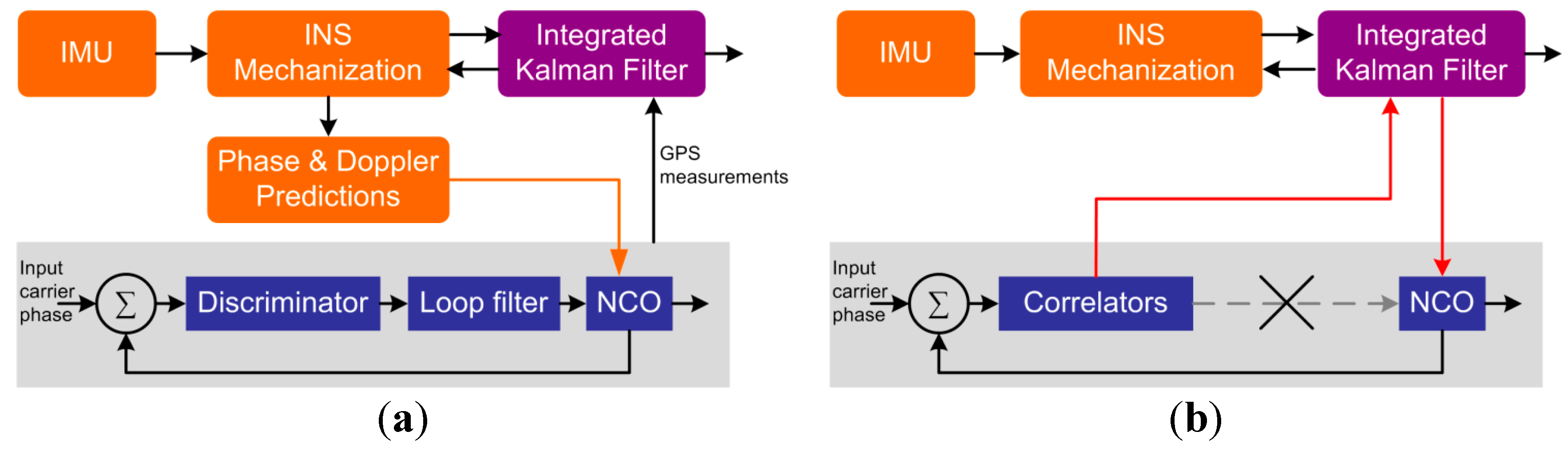
Based on the type of tracking loops used in receivers, the deeply coupled integration can be implemented in two different ways, which can be respectively named as scalar-based architecture and vector-based architecture [3], as shown in Figure 1. The scalar-based architecture refers to the individual tracking loops aided by INS [1]. Each individual tracking loop is comprised of a discriminator, a loop filter and a numerical controlled oscillator (NCO). The Kalman filter utilizes either raw measurement or processed positions and velocities from the receiver to update the INS periodically. The updated INS information is then given as feedback to correct the INS mechanization errors and inertial sensor errors. With the satellite ephemeris, the line-of-sight (LOS) Doppler from receiver to satellite can be predicted by the dynamic information from INS mechanization. When the estimated Doppler from INS is effective, both the Doppler aiding and the output of the loop filter are applied to adjust NCO.

By contrast, the vector-based architecture is considered as a vector-based receiver integrated with an inertial measurement unit (IMU), in which the traditional code and carrier tracking loops are eliminated. In vector-based architecture the traditional individual tracking loops are eliminated and it can make full use of the available information and get better signal sensitivity. However, individual carrier phase tracking loops are still used in vector-based architecture [4]. As a more simple approach, the scalar-based architecture, whose tracking loops are individual, is valuable for carrier phase tracking.

For the successful implementation of such systems, the inertial aiding information should have sufficient accuracy in short-term as the inertial aiding data can induce additional errors into the receiver tracking loops, especially for the low-end IMUs. Besides, the selection of IMU device should be seriously considered when designing a GPS/INS deep integration system. High grade of IMUs increase the costs while the low-end devices may lack the aiding ability. So it is important to evaluate the aiding information error and analyze the impacts of different grades of IMUs on the GPS receiver tracking loop.

Figure 1. Two architectures of GPS/INS deeply coupled integration. (a) Scalar-based architechture; (b) Vector-based architechture.

Figure 1. Two architectures of GPS/INS deeply coupled integration. (a) Scalar-based architechture; (b) Vector-based architechture.

1.1. Previous Work

Error propagation analysis is a combination of analysis and simulation techniques to evaluate navigation solution errors of different grades of INS [5]. The propagation of the errors can be represented in mathematical form as a set of differential equations which are derived from the system equations. Conventional error propagation analysis of the inertial navigation system mainly focus on the absolute accuracy which is dominated by the long-term and mid-term (e.g., several hours) position and attitude errors [5,6,7,8,9]. Even the ‘short-term’ analysis is still based on several hundred seconds scale [2]. Little work is made regarding the velocity accuracy in real short-term (e.g., typical GPS update interval, 1 s), which is specifically required in the deep integration system [10]. Besides, in a GPS/INS integrated system, the GPS updates can calibrate the inertial navigation system and limit the error drift. The conventional error propagation analysis is no longer a valid method to analyze the short-term accuracy of INS in deep integration system, especially for the case of low-end micro-electro-mechanical system (MEMS) INS.

Besides the theoretical error propagation analysis, different grades of IMU data (real or simulated) were also directly tested in the GPS/INS deep integration system to find out the real impact on receiver tracking loops. Gautier tested different grade of IMUs based on the GPS/INS Generalized evaluation tool (GIGET). Results showed that the navigation grade IMU enabled a lower tracking bandwidth and the automotive grade IMU only caused the tracking loop to become unstable [1]. Chiou [11] found that with continuous, high quality stand-alone GPS navigation measurements to blend with the inertial measurements, the quality of the IMU did not affect the accuracy of Doppler estimates; Yang [12] and Tsujii et al. [13] provided the similar conclusion that the system performance will be improved with the aiding of low-end IMUs. Petovello and O’Driscoll [4,14] have evaluated the channel filter performance of ultra-tight as a function of the IMU quality and the results showed that the IMU quality plays only a very small role in the expected tracking performance. Other simulation researches indicated that the low-end IMU was able to improve the performance of the receiver tracking loop [15,16,17,18,19]. The conclusions varied with different research platforms and test conditions.

Another way to analyze the impact of the inertial aiding information accuracy is to model the INS-aided tracking loops. Hemesath [20] proposed a mathematical structure of an inertially aided tracking loop in Laplace domain. The INS branch is simply modeled as the combination of scale factor (representing the accuracy of aiding information) and a first-order low-pass filter. In 2003, Alban [21] presented a simpler model of the INS aiding branch as just low-pass filter. Both of the models lack consideration of the IMU sensor errors and can not correctly reflect the error transformation of IMU in the tracking loop. Therefore, they can not be directly used for quantitative analysis of the impact of the IMU quality on the receiver tracking loop.

Generally speaking, the above methods lacked a comprehensive analysis on the relationship between the INS error sources and the receiver tracking error. They also did not make quantitative analysis of the impact of the different quality inertial aiding data in the short-term considering the GPS updates.

1.2. Objectives

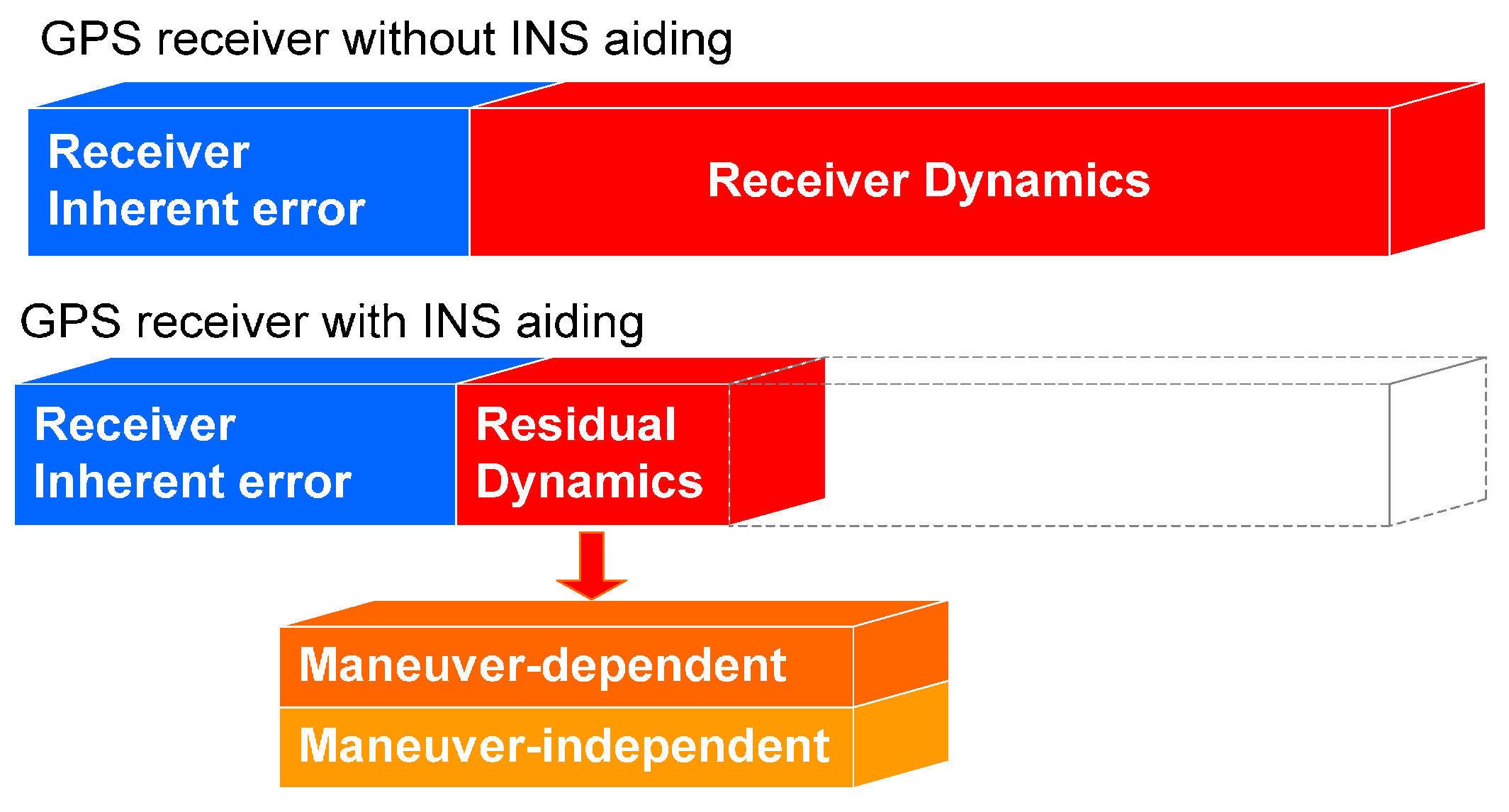
In practice, the INS aiding data is often in the form of velocity or Doppler estimation and the residual dynamics after the INS aiding are the velocity or Doppler estimation errors. With INS aiding, the residual dynamics which the tracking loops need to handle, can be divided into maneuver-dependent velocity error terms [5] and maneuver-independent velocity error terms (see Figure 2). The former refers to the INS solution errors caused by the receiver maneuvers, which can be regarded as the motion dynamic measurement leakage because of the INS dynamic errors. Considering the fact that the maneuver-dependent errors are much less than the maneuver itself, they are positive effects of the INS aiding. The maneuver-independent velocity error terms mean the velocity errors are irrelevant to the receiver dynamics (i.e., appears even when the vehicle stops), which can be regarded as the pure negative effect of the INS aiding to the receiver tracking loops [22].

Figure 2. The residual dynamics of the tracking loop with INS aiding.

Figure 2. The residual dynamics of the tracking loop with INS aiding.

In this paper, a quantitative analysis method is proposed to evaluate the impact of the maneuver-independent velocity errors of different grades of IMUs on the receiver PLLs in short-terms based on a scalar-based architecture. Compared with the previous works, the main novelty and advantage of the proposed method is to analyze the relationship between the error sources and the receiver tracking errors induced by different grades of IMUs in a quantitative way. The quantitative analysis can be a reference for the selection of inertial sensors when designing a GPS/INS deep integrated system.

The rest of this paper is organized as follows: firstly it presents detailed transfer relation of the IMU error sources and the INS maneuver-independent velocity errors in Laplace domain. The second section makes the time domain quantitative analysis of the maneuver-independent velocity errors caused by each individual IMU error source in short-term. In the third section, the impacts of the INS maneuver-independent velocity errors to the GPS PLLs are assessed. Finally, the conclusions of this study are given in the last section.

2. Methodology

This part starts with the INS error dynamic equations, which can be solved by the Laplace transform analysis. Then, the transfer relationship between the error sources and the velocity estimation errors can be achieved.

2.1. Error Dynamic Solutions of INS

Error dynamic equations are usually derived relating system performance to sources of error. The propagation of the errors can be represented as a set of difference equations which are derived from the system equations by taking partial derivatives [23].

$$\begin{array}{l}\delta {\dot{\mathit{r}}}^n=F_{rr}\delta {\mathit{r}}^n+F_{rv}\delta {\mathit{\nu }}^n\\ \delta {\dot{\mathit{v}}}^n\text{ = }{C}_b^n\cdot \delta {\mathit{f}}^b+C_b^n\cdot {\mathit{f}}^b\times {\mathbf{\varphi }}^n\\ -(2{\mathbf{\omega }}_{ie}^n+{\mathbf{\omega }}_{en}^n)\times \delta {\mathit{v}}^n+{\mathit{v}}^n\times (2\delta {\mathbf{\omega }}_{ie}^n+\delta {\mathbf{\omega }}_{en}^n)+\delta {\mathit{g}}^n\\ \dot{\mathbf{\varphi }}=F_{\text{ϕ}r}\cdot \delta {\mathit{r}}^n+F_{\text{ϕ}v}\cdot \delta {\mathit{v}}^n-[{\mathbf{\omega }}_{in}^n\times ]{\mathbf{\varphi }}^n-\delta {\mathbf{\omega }}_{ib}^n\end{array}$$

(1)

where

$$\begin{gathered} F_{rr}=\left(\begin{array}{ccc}0& 0& -\frac{v_N}{(R_M+h)}\\ \frac{v_E\sin L}{{(R_N+h)}^2{\cos }^{2}L}& 0& -\frac{v_E}{{(R_N+h)}^2\cos L}\\ 0& 0& 0\end{array}\right)F_{rv}=\left(\begin{array}{ccc}\frac{1}{R_M+h}& 0& 0\\ 0& \frac{1}{(R_N+h)\cos L}& 0\\ 0& 0& -1\end{array}\right) \\ {F}_{\text{ϕ}r}=\left(\begin{array}{ccc}-{\omega }_e\sin L& 0& -\frac{v_E}{{(R_N+h)}^2}\\ 0& 0& \frac{v_N}{{(R_M+h)}^2}\\ -{\omega }_e\cos L-\frac{v_E}{(R_N+h){\cos }^{2}L}& 0& \frac{v_E\tan L}{{(R_N+h)}^2}\end{array}\right)F_{\text{ϕ}v}=\left(\begin{array}{ccc}0& \frac{1}{R_N+h}& 0\\ -\frac{1}{R_M+h}& 0& 0\\ 0& -\frac{\tan L}{R_N+h}& 0\end{array}\right) \end{gathered}$$

All symbols in Equation (1) are defined as follows: operator δ means error of something, $\delta {\mathit{r}}^n$, $\delta {\mathit{v}}^n$ and ${\mathbf{\varphi }}^n$ are position, velocity and attitude error in the navigation frame respectively, $\delta {\mathit{f}}^b$ is the error for accelerometers and $\delta {\mathbf{\omega }}_{ib}^n$ is the error of gyros, ${\mathbf{\omega }}_e$ is the magnitude of the rotation rate of the Earth. $C_b^n$ is the rotation matrix from body frame (b-frame, Forward-Right-Down) to navigation frame (n-frame, North-East-Down), which represents the change of attitude. ${\mathit{f}}^b$ is the specific force in the b-frame (i.e., output of accelerometers), ${\mathbf{\omega }}_{ie}^n$ is the angular rate of e-frame relative to inertial frame (i-frame, nonrotating with respect to the Earth) in the n-frame, ${\mathbf{\omega }}_{en}^n$ is the angular rate of n-frame relative to e-frame in the n-frame, $\delta {\mathit{g}}^n$ is the normal gravity error in the local position in the n-frame, ${\mathbf{\omega }}_{ib}^b$ is the angular rate of b-frame relative to i-frame in b-the frame (i.e., output of gyros), ${\mathbf{\omega }}_{in}^b$ is the angular rate of n-frame relative to i-frame in b-frame, R_M, R_N are radii of curvature in the meridian and prime vertical, h is ellipsoidal height and L is geodetic latitude.

The complete forms of the error dynamic equations are complicated and it is hard to solve the equations directly. Some reasonable simplifications and assumptions can be achieved based on the peculiarity of the research objects:

(a)

It only needs to consider the stationary conditions (i.e., static and uniform rectilinear motion) as the main object of this paper is the maneuver-independent velocity error;

(b)

The minor terms (e.g., terms contain the reciprocal of the earth radius parameters) are ignored as they have little effect on the navigation errors;

(c)

The impact of position error can be ignored after simplification (as the left equations group in Equation (2)) because the position errors do not affect the velocity errors and attitude errors in the analysis;

(d)

Assume that the sensor selection of each axial is the same and it can be considered that the sensor errors characteristics in n-frame are the same with that in the b-frame, because the rotation matrix from b-frame to n-frame is an identity and orthogonal matrix.

Then the simplified error dynamic equations in n-frame can be expressed as:

$$\{\begin{array}{l}\delta \dot{L}=\delta {\nu }_N/\left(R_M+h\right)\\ \delta \dot{\lambda }=\delta {\nu }_E/(R_N+h)\cos L\\ \delta \dot{h}=-\delta {\nu }_D\\ \delta {\dot{v}}_N=-f_D^n{\text{ϕ}}_E+\delta f_N^n\\ \delta {\dot{v}}_E=f_D^n{\text{ϕ}}_N+\delta f_E^n\\ \delta {\dot{v}}_D=\delta f_D^n\\ {\dot{\text{ϕ}}}_N=-\delta {\omega }_N^n\\ {\dot{\text{ϕ}}}_E=-\delta {\omega }_E^n\\ {\dot{\text{ϕ}}}_D=-\delta {\omega }_D^n\end{array}\Rightarrow \{\begin{array}{l}\delta {\dot{v}}_N=-f_D^n{\text{ϕ}}_E+\delta f_N^n\\ \delta {\dot{v}}_E=f_D^n{\text{ϕ}}_N+\delta f_E^n\\ \delta {\dot{v}}_D=\delta f_D^n\\ {\dot{\text{ϕ}}}_N=-\delta {\omega }_N^n\\ {\dot{\text{ϕ}}}_E=-\delta {\omega }_E^n\\ {\dot{\text{ϕ}}}_D=-\delta {\omega }_D^n\end{array}$$

(2)

The simplified error dynamics can be expressed in matrix form as follows:

$$\left(\begin{array}{c}\delta {\dot{\nu }}_N\\ \delta {\dot{\nu }}_E\\ \delta {\dot{\nu }}_D\\ {\dot{\text{ϕ}}}_N\\ {\dot{\text{ϕ}}}_E\\ {\dot{\text{ϕ}}}_D\end{array}\right)=\mathit{F}\cdot \left(\begin{array}{c}\delta v_N\\ \delta v_E\\ \delta v_D\\ {\text{ϕ}}_N\\ {\text{ϕ}}_E\\ {\text{ϕ}}_D\end{array}\right)+\left(\begin{array}{c}\delta f_N^n\\ \delta f_E^n\\ \delta f_D^n\\ -\delta {\omega }_N^n\\ -\delta {\omega }_E^n\\ -\delta {\omega }_D^n\end{array}\right)\text{, }\mathit{F}=\left(\begin{array}{cccccc}0& 0& 0& 0& -f_D^n& 0\\ 0& 0& 0& f_D^n& 0& 0\\ 0& 0& 0& 0& 0& 0\\ 0& 0& 0& 0& 0& 0\\ 0& 0& 0& 0& 0& 0\\ 0& 0& 0& 0& 0& 0\end{array}\right)$$

(3)

Or simply expressed as vectors:

$$\dot{\mathit{x}}(t)=\mathit{F}(t)\mathit{x}(t)+\mathit{w}(t)$$

(4)

Here, the elements of F(t) are constant or changing slowly in short time, so the Laplace transform can be finished as [5,24]:

$$s\mathit{x}(s)=\mathit{F}\cdot \mathit{x}(s)+\mathit{x}(0)+\mathit{w}(s)\Rightarrow \mathit{x}(s)={(s\mathit{I}-\mathit{F})}^{-1}[\mathit{x}(0)+\mathit{w}(s)]$$

(5)

where I is identity matrix, x(0) is the initial value of x(t). Then the velocity error in Laplace domain can be derived from Equation (5).

$$\begin{array}{l}\delta v_N(s)=\frac{1}{s}\delta f_N^n(s)+\frac{f_D^n}{s^2}\delta {\omega }_E^n(s)+\frac{1}{s}\delta v_N(0)-\frac{f_D^n}{s^2}{\text{ϕ}}_E(0)\\ \delta v_E(s)=\frac{1}{s}\delta f_E^n(s)-\frac{f_D^n}{s^2}\delta {\omega }_N^n(s)+\frac{1}{s}\delta v_E(0)+\frac{f_D^n}{s^2}{\text{ϕ}}_N(0)\\ \delta v_D(s)=\frac{1}{s}\delta f_D^n(s)\text{+}\frac{1}{s}\delta v_D(0)\end{array}$$

(6)

where $\delta f_{*}^n(s)$ is the north accelerometer error, and $\delta {\omega }_{*}^n(s)$ is the gyro error; $\delta v_{*}(0)$ is the initial velocity error, ${\text{ϕ}}_{*}(0)$ is the initial attitude angle error. It should be noted that the initial errors in the GPS/INS integration system are the residual errors right after the GPS measurements update.

2.2. Detailed Modeling of the Error Sources in IMU

Equations (5) and (6) provide the solution of INS error dynamic equations; however, the sensor errors in Equation (6) are not specific enough for error propagation analysis. The sensor errors can be further modeled as bias and white-noise under stationary condition. The bias usually contains the constant part and random part. The random part of bias can be modeled as the first-order Gauss-Markov process [25].

$$\begin{array}{l}\delta \mathit{f}(t)={\mathit{b}}_a+{\mathit{w}}_a=\left[{\mathit{b}}_{a\_c}+G{M}_a(t)\right]+{\mathit{w}}_a(t)\\ \delta \mathbf{\omega }(t)={\mathit{b}}_g+{\mathit{w}}_g=\left[{\mathit{b}}_{g\_c}+G{M}_g(t)\right]+{\mathit{w}}_g(t)\end{array}$$

(7)

where

$$\stackrel{·}{GM}(t)=-\frac{1}{\mathit{T}}GM(t)+{\mathit{w}}_{GM}(t)$$

b_a, b_g are residual biases of the accelerometers and gyros, respectively, after the GPS update. w_a, w_g are the noise of the accelerometer and gyros, respectively, which are usually modeled by Gaussian white-noise. The bias generally consists of two parts, a constant part that can be modeled as random constant (i.e., b_{a_c} and b_{g_c} in Equation (7)) and a various part that can be modeled as first-order Gauss-Markov process (i.e., GM_a and GM_g in Equation (7)). T is the correlation time and w_GM is the driving noise of the Gauss-Markov process [26].

The Laplace transform of Equation (7) can be expressed as:

$$\begin{array}{l}\delta \mathit{f}(\text{s})=\left[\frac{{\mathit{b}}_{a\_c}}{s}+G{M}_a(s)\right]+{\mathit{w}}_a(s)=\left[\frac{{\mathit{b}}_{a\_c}}{s}+\frac{G{M}_a(0)+w_{GMa}(s)}{s+\frac{1}{T}}\right]+{\mathit{w}}_a(s)\\ \delta \mathbf{\omega }(s)=\left[\frac{{\mathit{b}}_{g\_c}}{s}+G{M}_g(s)\right]+{\mathit{w}}_g(s)=\left[\frac{{\mathit{b}}_{g\_c}}{s}+\frac{G{M}_g(0)+w_{GMg}(s)}{s+\frac{1}{T}}\right]+{\mathit{w}}_g(s)\end{array}$$

(8)

and GM(0) can be set as zero in numerical simulations.

Take the north direction as an example and, substituting the Laplace transform of Equation (8) into Equation (6), the relationship between the maneuver-independent velocity error of the north direction and every specific error sources can be established:

$$\delta v_N(s)=\frac{1}{s^2}{b}_{ax\_c}^n+\frac{1}{s}G{M}_{ax}^n(s)+\frac{1}{s}{w}_{ax}^n(s)+\frac{f_D^n}{s^3}{b}_{gy\_c}^n+\frac{f_D^n}{s^2}G{M}_{gy}^n(s)+\frac{f_D^n}{s^2}{w}_{gy}^n(s)+\frac{1}{s}\delta v_N(0)-\frac{f_D^n}{s^2}{\text{ϕ}}_E(0)$$

(9)

The maneuver-independent velocity errors of north direction caused by the various error sources can be expressed in the following equations. Equation (10) describes the relationship between the random constant error sources and the velocity errors directly; And the relationship between the noise error sources and the velocity errors are described as error transfer functions in Equation (11).

$$\{\begin{array}{l}\delta v_{N\_baxc}(s)=\frac{1}{s^2}{b}_{ax\_c}^n\\ \delta v_{N\_bgyc}(s)=\frac{f_D^n}{s^3}{b}_{gy\_c}^n\\ \delta v_{N\_\delta v_N(0)}(s)=\frac{1}{s}\delta v_N(0)\\ \delta v_{N\_{\text{ϕ}}_E(0)}(s)=-\frac{f_D^n}{s^2}{\text{ϕ}}_E(0)\end{array}$$

(10)

$$\{\begin{array}{l}{H}_{GMax}(s)=\frac{\delta v_{N\_GMax}(s)}{w_{GMax}^n(s)}=\frac{1}{s^2+\frac{1}{T}s}\\ H_{wax}(s)=\frac{\delta v_{N\_wax}(s)}{w_{ax}^n(s)}=\frac{1}{s}\\ H_{GMgy}(s)=\frac{\delta v_{N\_GMgy}(s)}{w_{GMgy}^n(s)}=\frac{f_D^n}{s^3+\frac{1}{T}{s}^2}\\ H_{wgy}(s)=\frac{\delta v_{N\_wgy}(s)}{w_{gy}^n(s)}=\frac{f_D^n}{s^2}\end{array}$$

(11)

Then, the maneuver-independent velocity errors caused by the constant errors sources (i.e., Equation (10)) can be achieved through inverse Laplace transform; and the maneuver-independent velocity errors caused by the white-noise driven errors (i.e., Equation (11)) will be achieved by Monte-Carlo [27] simulations as the expressions of the white-noise driven errors are not specific and it is hard to get the inverse Laplace transforms.

3. Quantitative Analysis of INS Velocity Errors

The equations above indicate that the error sources consist of the random constant driven errors (e.g., bias constant and initial navigation errors) in Equation (10) and the white-noise driven errors (e.g., sensor noise and Gauss-Markov processes) in Equation (11). The initial errors (i.e., $\delta v_N(0)$ and ${\text{ϕ}}_E(0)$) in the deep integration system should be the residual errors right after the GPS measurements update. In this section, the time domain response of the error sources of the maneuver-independent velocity errors will be presented, with some necessary real test data verification.

3.1. Quantitative Analysis Results in the Short Term

The time domain response of the random constant errors can be expressed by inverse Laplace transform of Equation (10) directly:

$$\{\begin{array}{l}\delta v_{N\_baxc}(t)=b_{ax\_c}^n\cdot t\\ \delta v_{N\_bgyc}(t)=\frac{1}{2}{f}_D^n{b}_{gy\_c}^n\cdot t^2\\ \delta v_{N\_\delta v_N(0)}(t)=\delta v_N(0)\\ \delta v_{N\_{\text{ϕ}}_E(0)}(t)=-f_D^n{\text{ϕ}}_E(0)\cdot t\end{array}$$

(12)

The error components driven by white-noise are too complicated to get their time domain expression by the inverse Laplace transform, and therefore Monte-Carlo simulations are used to analyze their time domain response based on the transfer function provided in Equation (11). Quantitative analysis of the maneuver-independent velocity errors, which represent the quality of aiding data, can be achieved based on the time domain response analysis.

Before the quantitative analysis, representative MEMS IMU (MTi-G, Xsens, Enschede, The Netherlands) [28] and tactical IMU (SPAN-FSAS, Novatel, Calgary, AB, Canada) [29] specifications of the error sources are listed in Table 1 and the sources of the parameters are described as below:

(a)

The parameters are obtained based on real GPS/INS data processing and the inertial sensors specifications; and the GPS measurements are single point positioning results;

(b)

The bias constants are the statistics of the standard deviation of the bias estimation right after the GPS update;

(c)

The initial errors are the statistics of the navigation errors right after the GPS update;

(d)

The other parameters are set according to the real data process parameters.

Table 1. Specifications of typical inertial measurement units (IMUS).

Characteristics		Inertial Measurement Unit IMU
		MTi-G	SPAN-FSAS
Grade		MEMS	Tactical Frade
Gyro	Mean squared value of bias drift (σ)	100 deg/h	0.1 deg/h
	Correlation time (T)	600 s	10,800 s
	Gyro white-noise (ARW)	3 deg/h	0.15 deg/h
Accel	Mean squared value of bias drift (σ)	2000 mGal	100 mGal
	Correlation time (T)	600 s	10,800 s
	Accel. white-noise (VRW)	0.12 m/s/h	0.03 m/s/h
Gyro bias Constant ( bg*_c) *		15 deg/h	0.1 deg/h
Accel. bias Constant ( ba*_c) *		800 mGal	50 mGal
Initial velocity error $\delta v_N(0)$ **		0.04 m/s	0.025 m/s
Initial attitude error ${\text{ϕ}}_E(0)$ **		0.3 deg	0.015 deg

Notes: * Residual bias errors after GPS update; ** Residual navigation errors after GPS update.

Table 1. Specifications of typical inertial measurement units (IMUS).

Characteristics		Inertial Measurement Unit IMU
		MTi-G	SPAN-FSAS
Grade		MEMS	Tactical Frade
Gyro	Mean squared value of bias drift (σ)	100 deg/h	0.1 deg/h
	Correlation time (T)	600 s	10,800 s
	Gyro white-noise (ARW)	3 deg/h	0.15 deg/h
Accel	Mean squared value of bias drift (σ)	2000 mGal	100 mGal
	Correlation time (T)	600 s	10,800 s
	Accel. white-noise (VRW)	0.12 m/s/h	0.03 m/s/h
Gyro bias Constant ( bg*_c) *		15 deg/h	0.1 deg/h
Accel. bias Constant ( ba*_c) *		800 mGal	50 mGal
Initial velocity error $\delta v_N(0)$ **		0.04 m/s	0.025 m/s
Initial attitude error ${\text{ϕ}}_E(0)$ **		0.3 deg	0.015 deg

Notes: * Residual bias errors after GPS update; ** Residual navigation errors after GPS update.

Substituting the parameters into the time response expressions and the Monte-Carlo simulations, the quantitative maneuver-independent velocity errors of all error sources can be achieved. In the Monte-Carlo simulations of the white-noise driven error sources, more than a thousand samples are simulated based on the parameters of the IMUs and the statistic results are presented in the flowing figures.

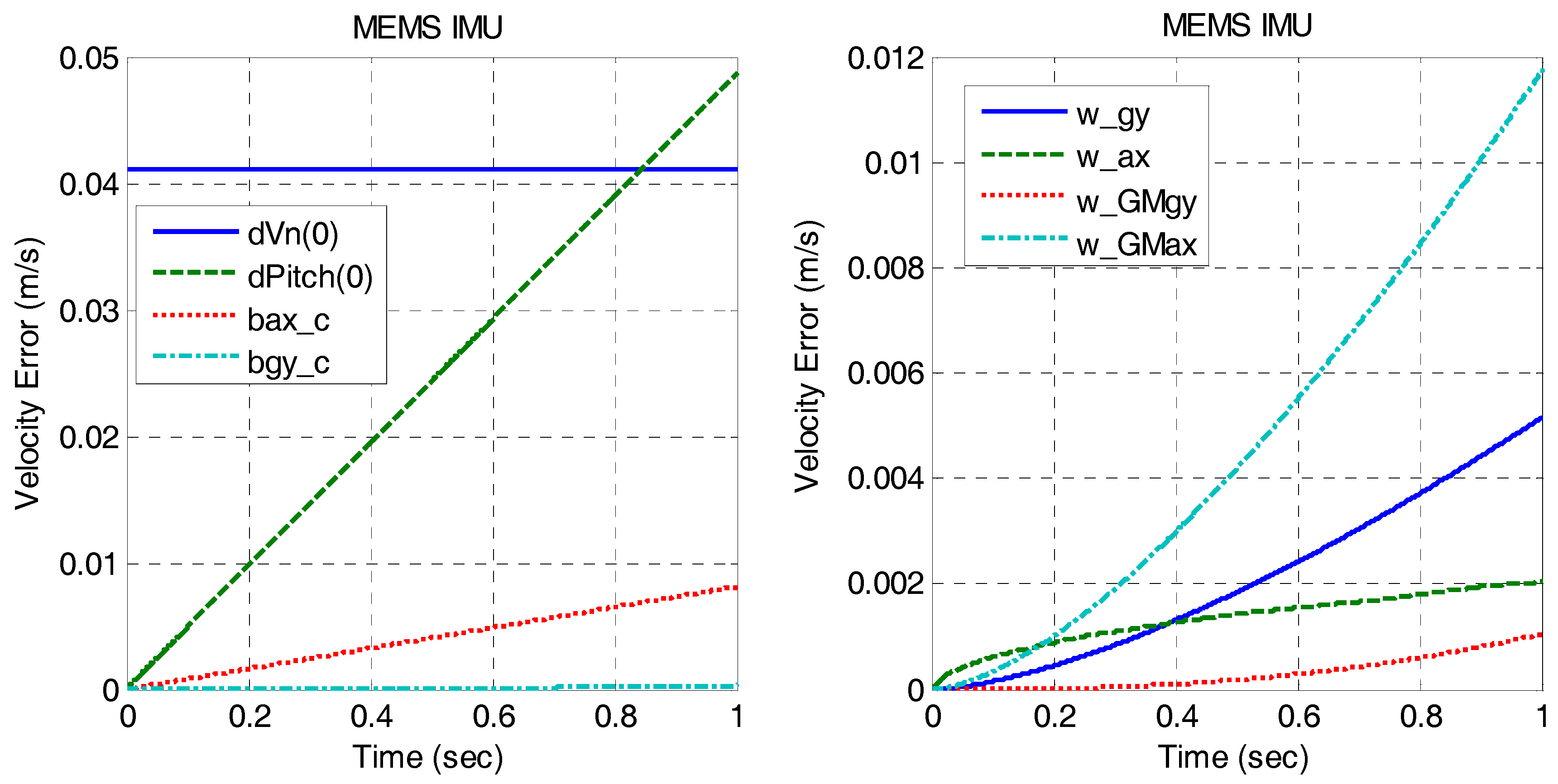
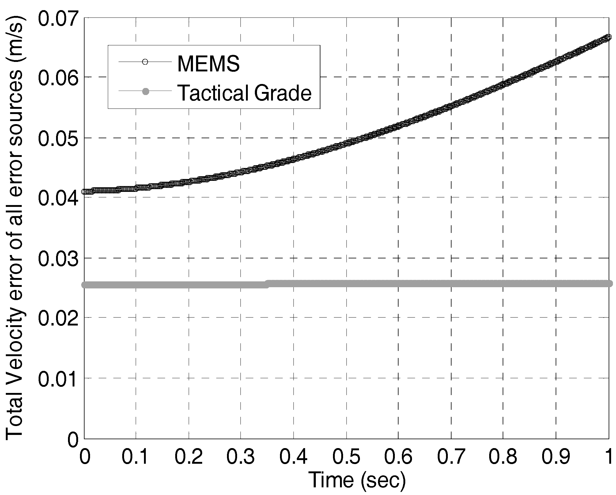
Figure 3 and Figure 4 show the time response of the INS velocity error caused by each random constant errors and white-noise driven errors of MEMS and tactical grade IMUs in short-term (i.e., 1 s) respectively. Figure 5 presents the total maneuver-independent velocity errors caused by all error sources of the MEMS and tactical IMUs. The figures show the positive errors as the time responses are statistic results.

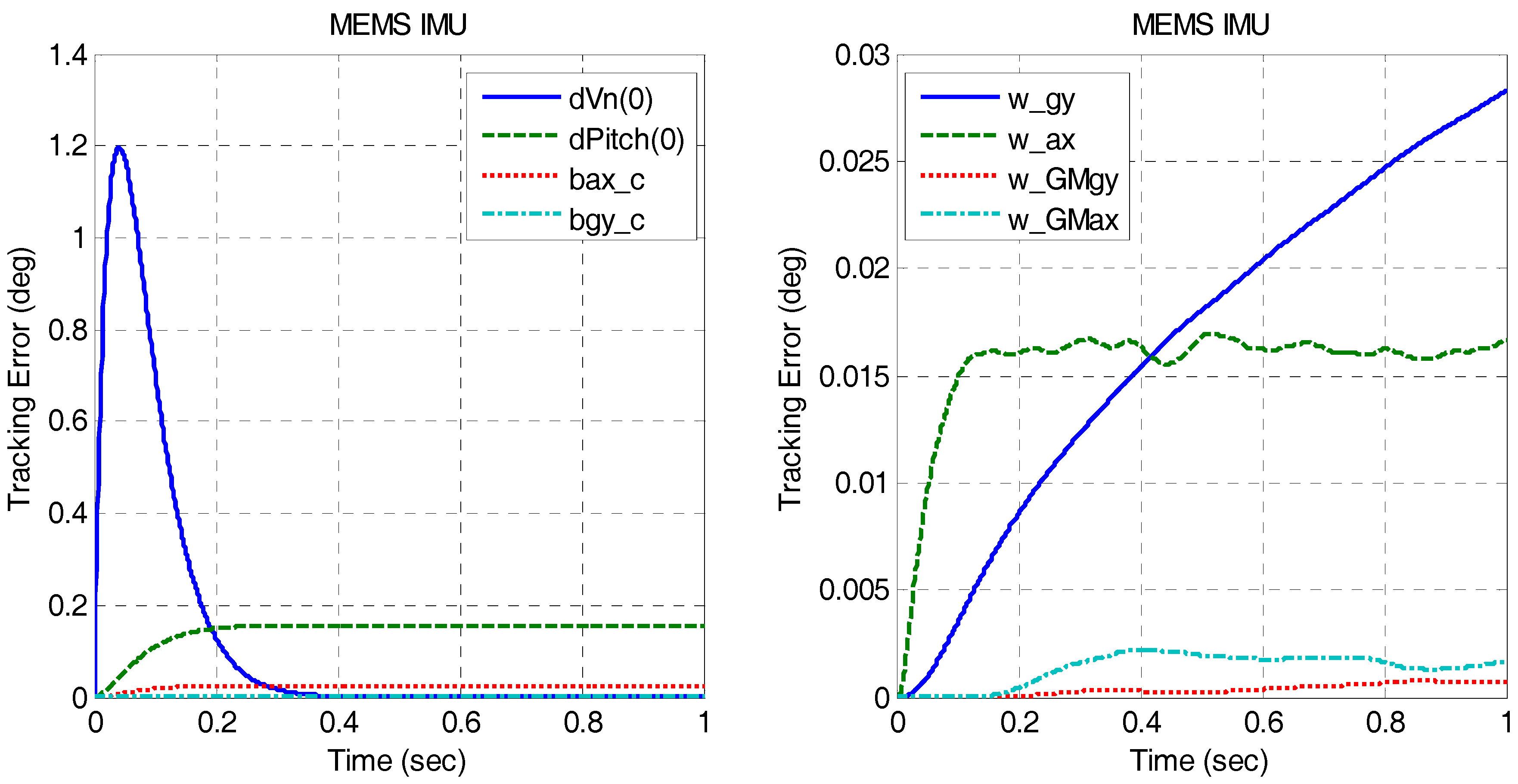
Figure 3. The quantitative velocity errors caused by micro-electro-mechanical system (MEMS) INS error sources.

Figure 3. The quantitative velocity errors caused by micro-electro-mechanical system (MEMS) INS error sources.

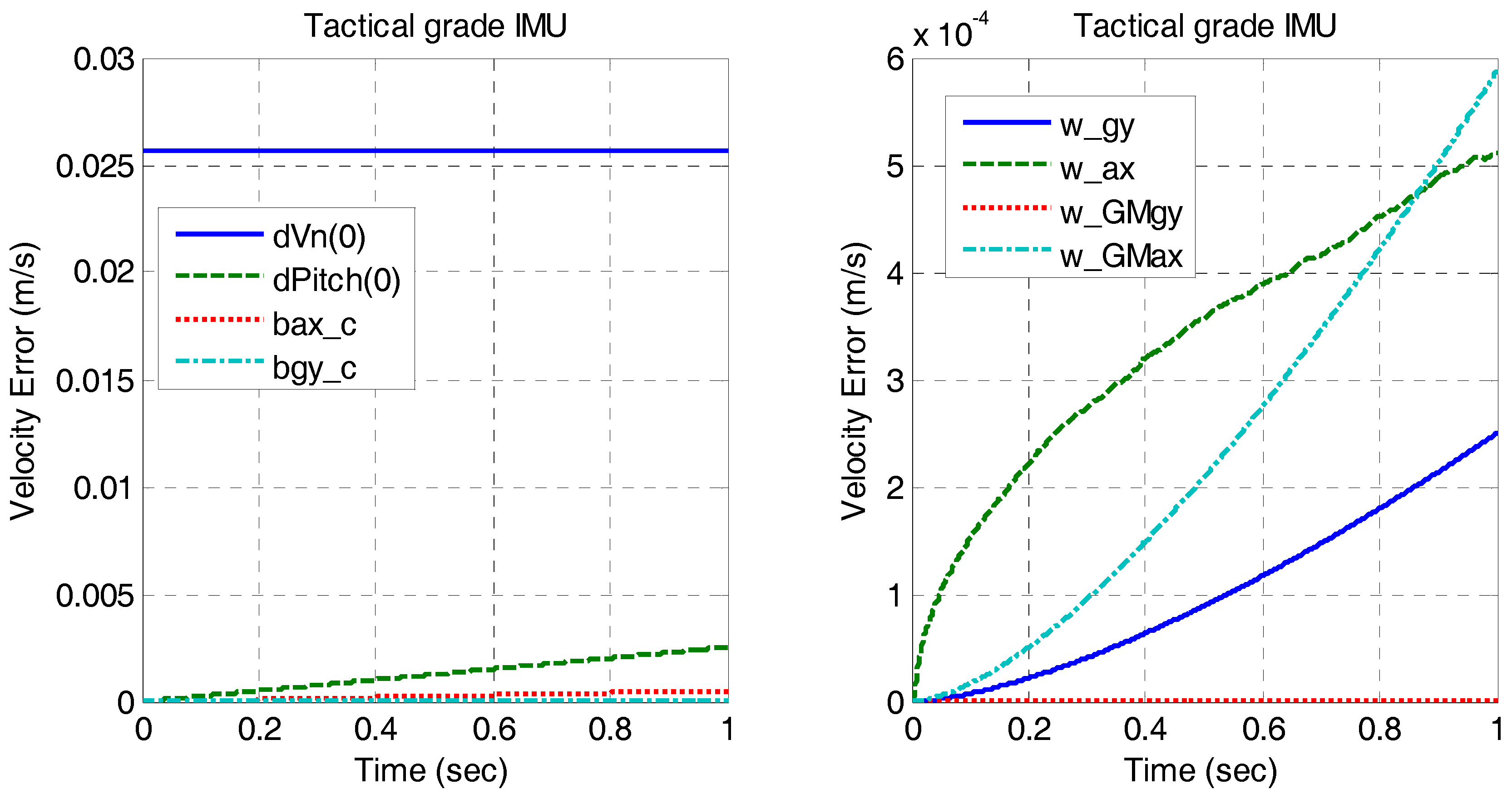
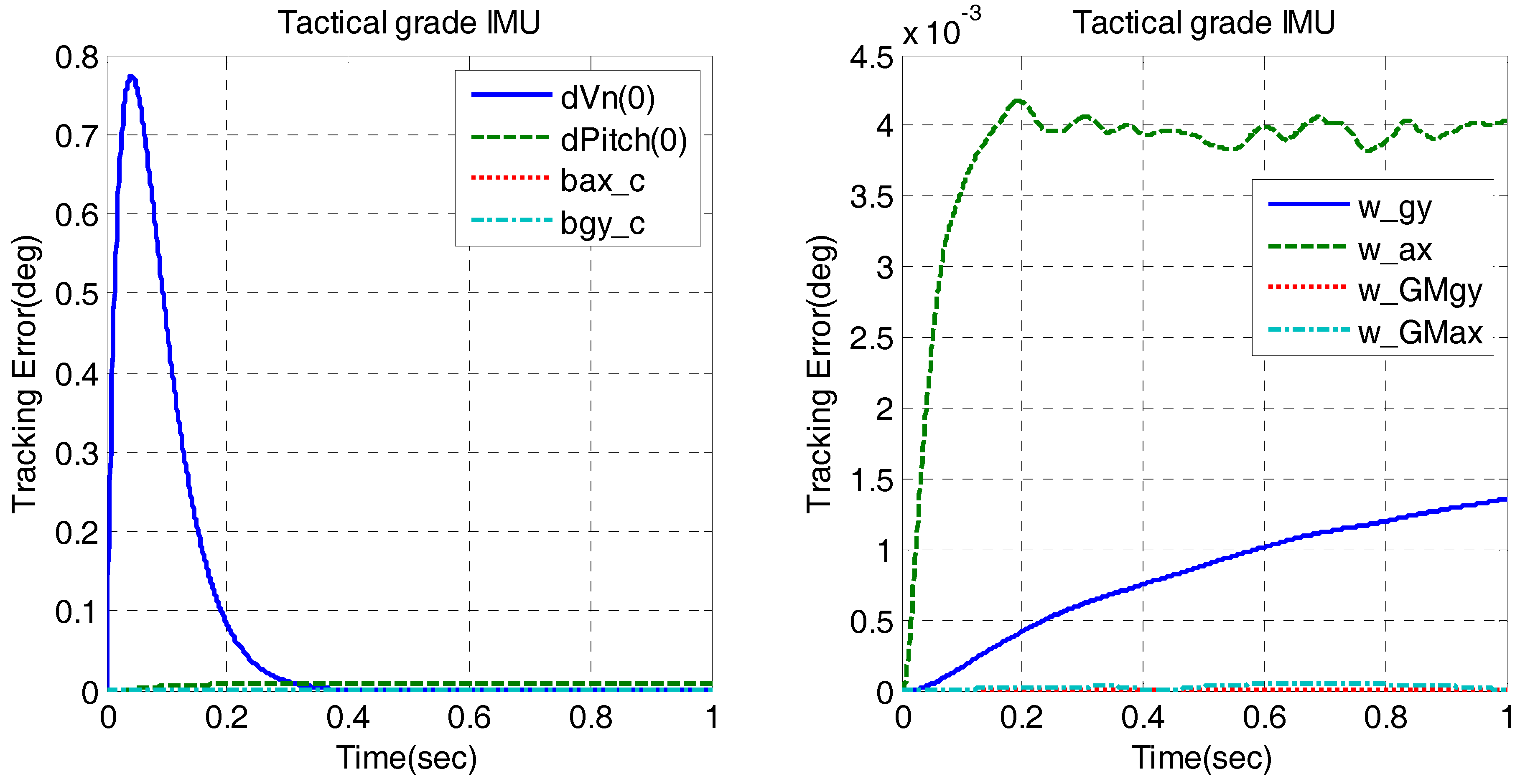
Figure 4. The quantitative velocity errors caused by tactical grade INS error sources.

Figure 4. The quantitative velocity errors caused by tactical grade INS error sources.

Figure 3 and Figure 4 indicate that the initial errors (i.e., initial velocity error and initial attitude error) are the main factors which affect the total maneuver-independent velocity error most. The initial velocity error basically determines the start of the velocity error drift and the initial attitude error (e.g., pitch error) and the accelerometer bias constant determine the trend of the velocity drift. The velocity error of tactical grade INS drifts much slower than that of the MEMS INS as it has better accuracy of the initial attitude and lower accelerometer bias constant.

Figure 5 also shows that the total maneuver-independent velocity errors of MEMS and tactical grade INS are less than 0.1 m/s and 0.03 m/s, respectively, within one second (the typical GPS update interval). Usually, the vehicle velocity can be dozens meters per second and the conventional receiver tracking loop needs to track all the dynamic stress. However, with the INS aiding, the tracking loop only needs to track the residual dynamics, such as the maneuver-independent velocity errors, which is far less than the dynamic itself.

Figure 5. The total maneuver-independent velocity errors caused by all error sources.

Figure 5. The total maneuver-independent velocity errors caused by all error sources.

3.2. Real Tests Validation of the INS Velocity Errors

In order to validate the quantitative results of the maneuver-independent velocity errors above, real tests data analysis has been performed.

Two sets of road tests were conducted in Wuhan in June 2013. The Xsens MTi-G module was chosen as representative low-end MEMS system and Novatel SPAN-FSAS was the typical tactical grade system. A navigation grade GPS/INS system was involved to provide the reference truth. The collected IMU data and GPS single point positioning (SPP) solutions were post-processed by integration algorithm and error analysis to determine the final solutions.

In order to get the maneuver-independent velocity errors of INS from the real test data, the velocity error of all the non-maneuver portions (e.g., static and uniform rectilinear motion) were picked and divided into segments of 1 s at the GPS update epochs. Then the velocity error drifts in these segments were summarized statistically, as shown in Figure 6, which reflected the drift level of the velocity errors of the INS during the GPS update interval. Here we use the north direction error as example.

Figure 6. The maneuver-independent velocity errors of the real tests data from different grades of IMUs comparing to theoretical analysis results.

Figure 6. The maneuver-independent velocity errors of the real tests data from different grades of IMUs comparing to theoretical analysis results.

The black curves in Figure 6 are the quantitative analysis results from subsection 3.1 and the color curves are the statistical results of velocity error of real test data. The figure shows that the statistic results of the real tests are generally consistent with the time domain response analysis results. And it validates the results of the quantitative analysis of the INS maneuver-independent velocity errors.

The analysis above has focused on the quality of the aiding data introduced by different grades of INS under stationary conditions. Although results have indicated that the maneuver-independent velocity errors were small (less than half Hertz in Doppler), analysis should be further performed to evaluate the exact impact of the aiding errors from different grades of INS to the carrier phase measurement in the GPS receiver tracking loop.

4. Quantitative Error Analysis in GPS Tracking Loop

The INS maneuver-independent velocity errors caused by different IMU error sources have been analyzed and verified in Section 2 and Section 3 in Laplace domain and time domain respectively. This section will feed the INS aiding velocity (i.e., Doppler aiding) into the GPS tracking loop and analyze the consequent carrier phase tracking performance.

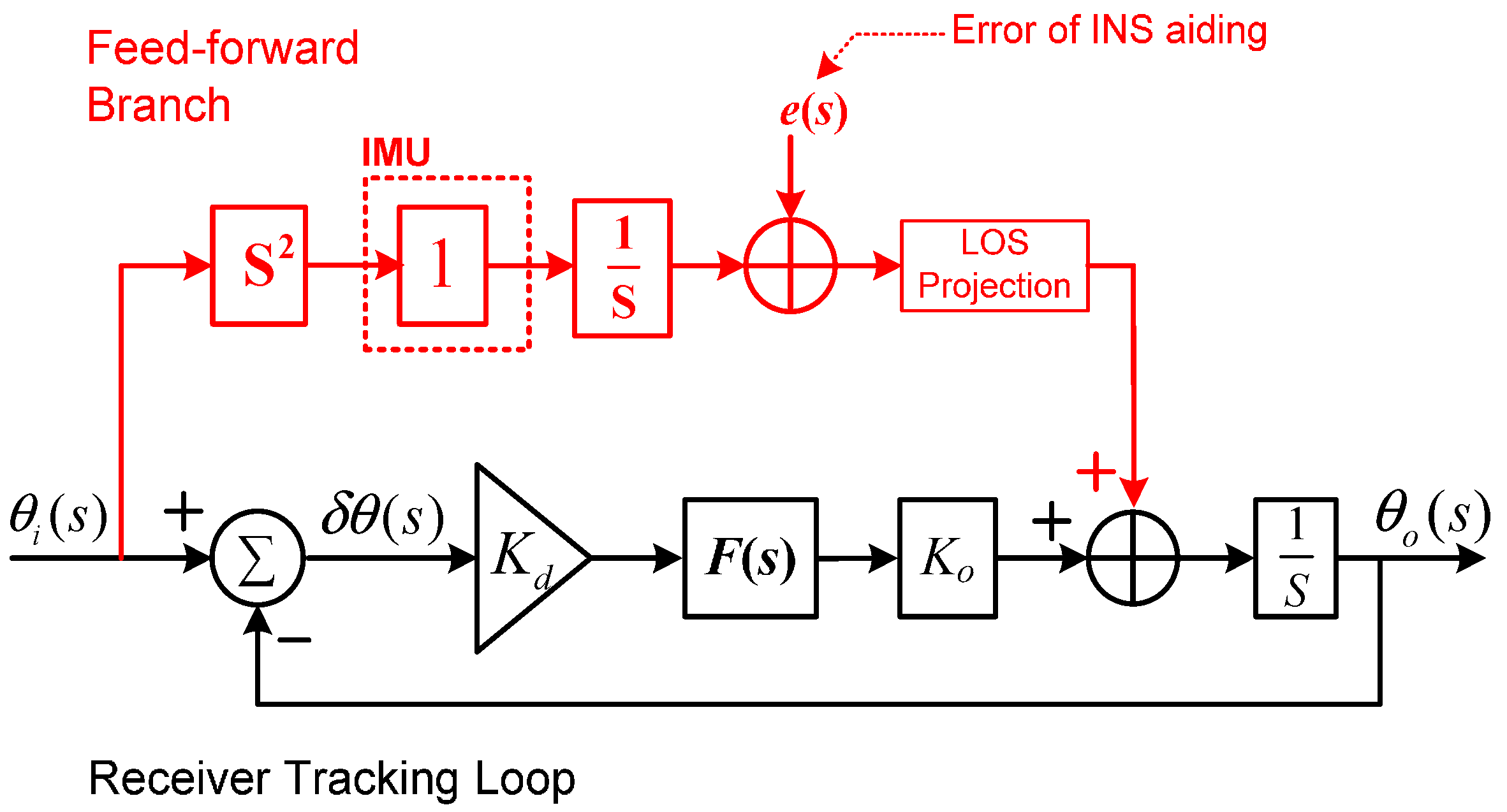
Figure 7 presents a mathematical model of GPS receiver tracking loop with INS aiding in Laplace domain [30]. The inertial aiding information can be induced into the tracking loop as a feed-forward branch. ${\theta }_i(s)$ is the phase of input signal, ${\theta }_o(s)$ is the output phase, $\delta \theta (s)$ is the phase tracking error, $K_d$ is gain of the discriminator, $\mathit{F}(s)$ is the transfer function of the loop filter, $K_o$ is the gain of NCO, and $\mathit{e}(s)$ here represents the maneuver-independent error vector of the aiding data.

Figure 7. Mathematical model of GPS receiver tracking loop with INS aiding.

Figure 7. Mathematical model of GPS receiver tracking loop with INS aiding.

The Doppler frequency of the carrier signal can be expressed simply as the velocity of the receiver relative to the satellite, projected onto the LOS direction. In order to analyze the worst influence of the maneuver-independent velocity errors on the receiver tracking loop, we assume that the satellite is right at the north direction of the receiver (i.e., the maximum projection of the error); and then evaluate the impact of the north velocity error on the satellite signal carrier phase errors estimated by GPS receiver.

Take the 2nd-order tracking loop as an example, the system transfer function in Laplace domain can be described as follows [31,32]:

$$H(s)=\frac{2\xi {\omega }_{n}s+{\omega }_n^2}{s^2+2\xi {\omega }_{n}s+{\omega }_n^2}$$

(13)

where, ${\omega }_n$ is the natural radian frequency of the loop filter, ξ is the damping factor.

The Doppler aiding error caused by the INS maneuver-independent velocity error can be presented as:

$$\begin{array}{l}\delta A(s)=\frac{2\pi }{\lambda }\cdot e(s)\\ =\frac{2\pi }{\lambda }\cdot [\frac{1}{s^2}{b}_{ax\_c}^n+\frac{1}{s}G{M}_{ax}^n(s)+\frac{1}{s}{w}_{ax}^n(s)+\frac{f_D^n}{s^3}{b}_{gy\_c}^n\\ +\frac{f_D^n}{s^2}G{M}_{gy}^n(s)+\frac{f_D^n}{s^2}{w}_{gy}^n(s)+\frac{1}{s}\delta v_N(0)-\frac{f_D^n}{s^2}{\text{ϕ}}_E(0)]\end{array}$$

(14)

where, λ is the wavelength of GPS carrier. Then the tracking error of the GPS receiver loop caused by INS maneuver-independent velocity error will be:

$$\delta \theta (s)=-\frac{1}{s}\delta A(s)\left[1-H(s)\right]$$

(15)

Substituting the INS Doppler aiding errors in Laplace domain (i.e., Equation (14)) into Equation (15), then the relation between the maneuver-independent velocity errors sources and the tracking errors can be expressed as follows:

$$\{\begin{array}{l}\delta {\theta }_{b_{ax\_c}}(s)=-\frac{2\pi }{\lambda }\cdot \frac{\frac{b_{ax\_c}^n}{s}}{s^2+2\xi {\omega }_{n}s+{\omega }_n^2}\\ \delta {\theta }_{b_{gy\_c}}(s)=-\frac{2\pi }{\lambda }\cdot \frac{f_D^n}{s}\cdot \frac{\frac{b_{gy\_c}^n}{s}}{s^2+2\xi {\omega }_{n}s+{\omega }_n^2}\\ \delta {\theta }_{\delta v_N(0)}(s)=-\frac{2\pi }{\lambda }\cdot \frac{\delta v_N(0)}{s^2+2\xi {\omega }_{n}s+{\omega }_n^2}\\ \delta {\theta }_{{\text{ϕ}}_E(0)}(s)=\frac{2\pi }{\lambda }\cdot f_D^n\cdot \frac{\frac{{\text{ϕ}}_E(0)}{s}}{s^2+2\xi {\omega }_{n}s+{\omega }_n^2}\end{array}$$

(16)

$$\{\begin{array}{l}{H}_{\delta \theta \_GMax}(s)=\frac{\delta {\theta }_{GMax}(s)}{w_{GMax}(s)}=-\frac{2\pi }{\lambda }\cdot \frac{1}{s^2+2\xi {\omega }_{n}s+{\omega }_n^2}\cdot \frac{1}{s+\frac{1}{T}}\\ H_{\delta \theta \_w_{ax}}(s)=\frac{\delta {\theta }_{w_{ax}}(s)}{w_{ax}(s)}=-\frac{2\pi }{\lambda }\cdot \frac{1}{s^2+2\xi {\omega }_{n}s+{\omega }_n^2}\\ H_{\delta \theta \_GMgy}(s)=\frac{\delta {\theta }_{GMgy}(s)}{w_{GMgy}(s)}=-\frac{2\pi }{\lambda }\cdot \frac{1}{s}\cdot \frac{f_D^n}{s^2+2\xi {\omega }_{n}s+{\omega }_n^2}\cdot \frac{1}{s+\frac{1}{T}}\\ H_{\delta \theta \_w_{gy}}(s)=\frac{\delta {\theta }_{w_{gy}}(s)}{w_{gy}(s)}=-\frac{2\pi }{\lambda }\cdot \frac{1}{s}\cdot \frac{f_D^n}{s^2+2\xi {\omega }_{n}s+{\omega }_n^2}\end{array}$$

(17)

For analysis convenience, the damping factor ξ is set to a typical value (e.g., ξ = 1), the bandwidth of the tracking loop is set 15 Hz and take GPS L1 (i.e., wavelength λ = 0.19 m) as example. Using the same analysis strategies as in the previous section, quantitative analysis to the impact of different grades of INS to the carrier phase measurement can be achieved by the inverse Laplace transform and Monte Carlo simulations, which are presented in Figure 8 and Figure 9.

Figure 8. Carrier phase tracking errors caused by the maneuver-independent velocity error sources of MEMS IMU.

Figure 8. Carrier phase tracking errors caused by the maneuver-independent velocity error sources of MEMS IMU.

Figure 9. Carrier phase tracking errors caused by the maneuver-independent velocity error sources of tactical grade IMU.

Figure 9. Carrier phase tracking errors caused by the maneuver-independent velocity error sources of tactical grade IMU.

Results show that the initial errors (i.e., initial velocity error and the initial attitude error right after the GPS update) are still the main factors which affect the tracking errors. The initial attitude error of the tactical grade IMU has less impact to the carrier phase measurement compared with the MEMS IMU.

Figure 10 presents the total tracking errors caused by the maneuver-independent velocity errors of different grade of IMUs. The carrier phase tracking error caused by the maneuver-independent velocity errors of MEMS INS is less than 1.2 degrees in total, while the tracking error caused by the maneuver-independent velocity errors of tactical grade IMU is less than 0.8 degrees. Compared with the carrier phase error caused by the receiver inherent error sources (e.g., the oscillator error and thermal noise), which will be several degrees [32], this negative effect is small enough to be tolerated by the receiver tracking loop. Even the MEMS INS is qualified for GPS/INS deep integration.

Figure 10. Total carrier phase tracking errors caused by the maneuver-independent velocity errors of different grades of IMUs.

Figure 10. Total carrier phase tracking errors caused by the maneuver-independent velocity errors of different grades of IMUs.

To keep our conclusion more universal, it is worth noting the following explanations:

(1)

The quantitative analysis given in this paper is based on a set of assumptions such as the IMU parameters, design parameters of the INS aiding loop, etc., which are essential to make the analysis feasible. We have chosen the most typical cases.

(2)

The 2nd order tracking loop was used as example. However the 3rd order loop won’t perform much different since the initial velocity error, which can be regarded as Doppler step input to the loop, is the dominant factor.

5. Conclusions

This paper presented a quantitative analysis on the impacts of the aiding information from different grades of IMUs in GPS/INS deep integration. Based on the fact that even low-end MEMS INS can sense the major part of the vehicle motion variations and block most of the dynamic stress for the GPS tracking loop, the positive effect of the INS aiding has been well recognized. Therefore, this paper focused on the negative effect of the inertial aiding, i.e., the tracking error caused by the maneuver-independent velocity error of INS. The analysis used the Laplace transform to solve the simplified error dynamic equations of INS to evaluate the maneuver-independent velocity error of the INS aiding; then, the time domain responses of the consequent carrier phase tracking errors were derived quantitatively by the inverse Laplace transform and Monte-Carlo simulations.

Results showed that the maneuver-independent velocity errors induced by the INS are relatively small (below 0.1 m/s for MEMS case and 0.08 m/s for tactical grade IMU case) in the typical GPS update interval (i.e., 1 s), which was confirmed by the real test results in the paper. After inducing the INS aiding data into the GPS tracking loop, the consequent carrier phase tracking error in the short-term was below 1.2 degrees for the case of MEMS IMU and 0.8 degrees for the case of tactical grade IMU, which is much less then that caused by the receiver inherent errors (including the oscillator error and the thermal noise).

The analysis results indicate that even the low-end MEMS IMU has the ability to provide the aiding information with sufficient quality for the GNSS signal tracking purpose. There is no significant difference for different grades of IMUs when GNSS signals are continuous and stable, because the low-end MEMS IMU has provided good enough Doppler aiding to the GNSS tracking loop. However, the higher grade (e.g., tactical grade) IMUs have smaller drift errors and may have potential for the open loop tracking and re-acquisition of GPS receiver when suffering signal attenuation and blockage. The quantitative analysis results can guide the selection of the inertial sensors for GPS/INS deep integration system.

It should be noted that the analysis in this paper focused on the short-term (i.e., 1 s) performance of the INS aiding for the GPS signal tracking with continuous GPS update. It does not apply to the long-term cases, such as GPS outages and INS aided re-acquisition.