Mori-Tanaka Based Estimates of Effective Thermal Conductivity of Various Engineering Materials

Abstract

The purpose of this paper is to present a simple micromechanics-based model to estimate the effective thermal conductivity of macroscopically isotropic materials of matrix-inclusion type. The methodology is based on the well-established Mori-Tanaka method for composite media reinforced with ellipsoidal inclusions, extended to account for imperfect thermal contact at the matrix-inclusion interface, random orientation of particles and particle size distribution. Using simple ensemble averaging arguments, we show that the Mori-Tanaka relations are still applicable for these complex systems, provided that the inclusion conductivity is appropriately modified. Such conclusion is supported by the verification of the model against a detailed finite-element study as well as its validation against experimental data for a wide range of engineering material systems.

1. Introduction

There has been a clear trend over the last decade to exploit ever greater detail of the material structure to better predict material response from simulations. Hierarchical modeling strategy, either coupled or uncoupled and mostly of the bottom-up type, has served to provide estimates of the macroscopic response. In this process, geometric details decisive for a given scale are first quantified by employing various statistical descriptors [1] but eventually smeared via homogenization to render larger scale property. Greater precision is expected when introducing the results of microstructure evaluation into the homogenization step. However, the actual gain when compared to the cost of this analysis is still in question. Obviously, description of evolving microstructures or rigorous representation of deformation mechanisms would require to account for almost every detail of the microstructure on a given scale. But how deep do we have to go if only the effective macroscopic response (i.e., linear macroscopic properties) is of the primary interest? Such a goal is addressed in this contribution.

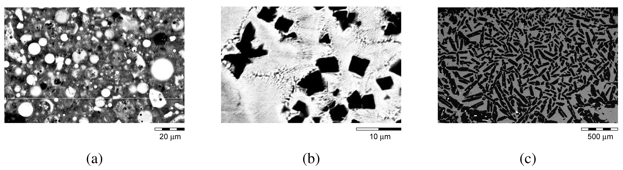
Here, the modeling effort concentrates on the evaluation of effective thermal conductivities of various engineering materials with a significant degree of heterogeneity focusing on imperfect thermal contact along constituents interfaces. We shall argue, shielded by available experimental data, that reasonably accurate predictions of macroscopic response can be obtained with very limited information about actual microstructure such as volume fractions and local properties of material phases. Consequently, we lump the entire analysis on the assumption of representing true material structures by statistically isotropic distribution of spheres. Figure 1 shows micro-images of selected material representatives which seem to admit this classification. Note that whatever material phase embedded into the matrix (the basic material) is henceforth termed the heterogeneity in real material systems while it is termed inclusion in approximations adopted for calculations.

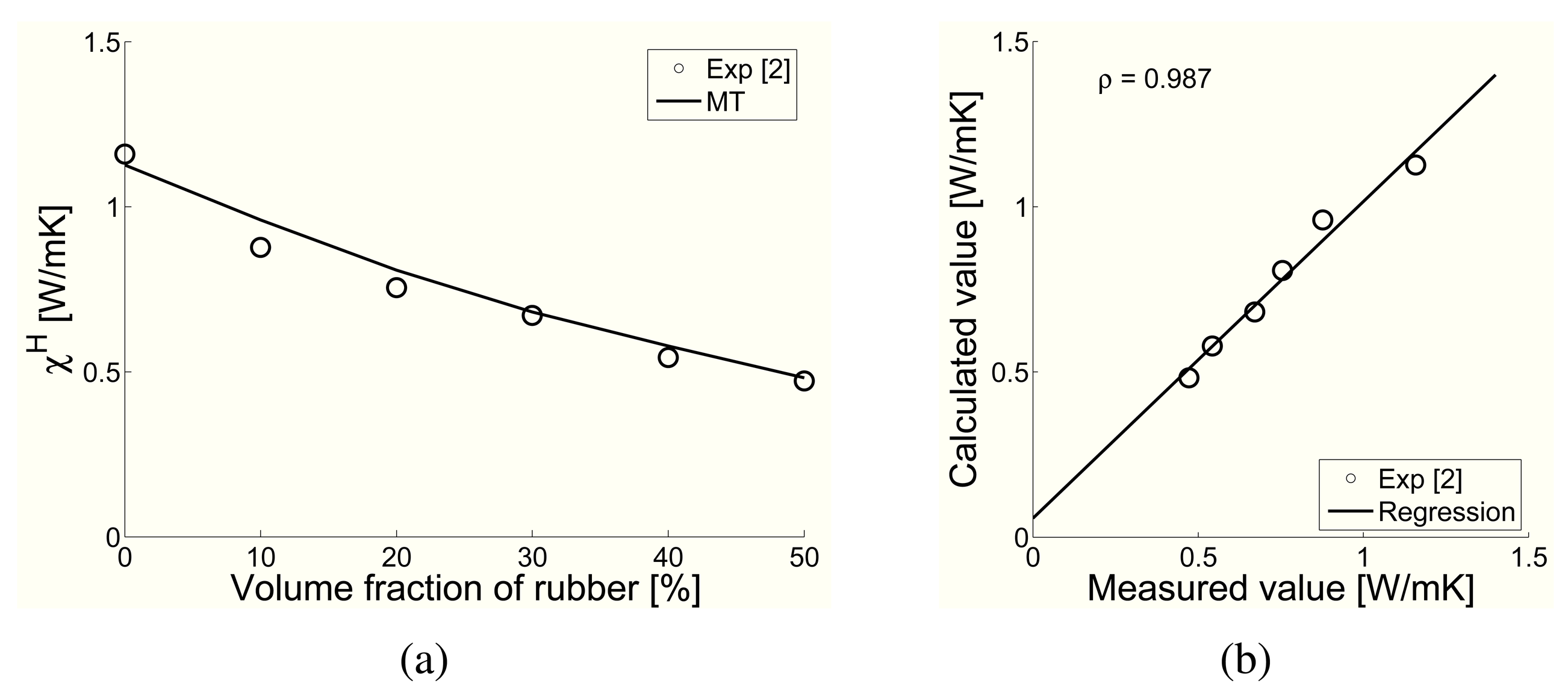
Strong motivation for this seemingly swingeing simplification is supported by experimental measurements presented in [2] for cement matrix based mixture of rubber particles and air voids. Comparison between experimental data and predictions provided by the Mori-Tanaka averaging scheme under the premise of random distribution of spherical inclusions appears in Figure 2. The match is almost remarkable.

Going back to Figure 1 one may object that while admissible for Figure 1(a) the spherical approximation of particle phase in Figure 1(c) will yield rather erroneous predictions. Note, however, that this attempt is not hopeless providing the microstructure can still be considered as macroscopically isotropic, which ensures the statistically isotropic distribution of heterogeneities having isotropic material symmetry. In that case, it can be shown that the previously mentioned Mori-Tanaka method written out for spherical inclusions is adequate provided that the material properties of the inclusions are suitably modified. Although this step requires information beyond that of volume fractions of phases, the benefit of gathering additional data will become particularly appreciable once we turn our attention to material systems with imperfect interfaces, which is the principal objective of this study.

The problem of quantifying the influence of imperfect thermal contact on the overall thermal conductivity has been under intense study in the past. Hasselman and Johnson [3] provided estimates for dilute concentration of mono-disperse spherical and cylindrical heterogeneities. Successful application of this simple model to Al/SiC porous composites is presented in [4]. The Hasselman-Johnson results were then extended by Benveniste and Miloh [5] to spheroidal particle shapes with imperfect interfaces and subsequently applied in the framework of the Mori-Tanaka method [6]. These early developments were later generalized by Nogales and Böhm, who proposed in [7] a simple method for dealing with polydisperse systems of spherical particles. In addition, rigorous third-order bounds for effective conductivity of macroscopically isotropic distribution of particles with imperfect interfaces were derived by Torquato and Rintoul [8]. Alternatively, as demonstrated by Hashin [9], the material systems with imperfect interfaces can be accurately approximated by the coated inclusion model developed by Dunn and Taya [10], which also accounts for different orientation of the inclusions. When attention is limited to spherical inclusions, the results presented in [7] can be obtained in a very elegant way by simple extension of one-dimensional analysis. This is demonstrated in Appendix B.

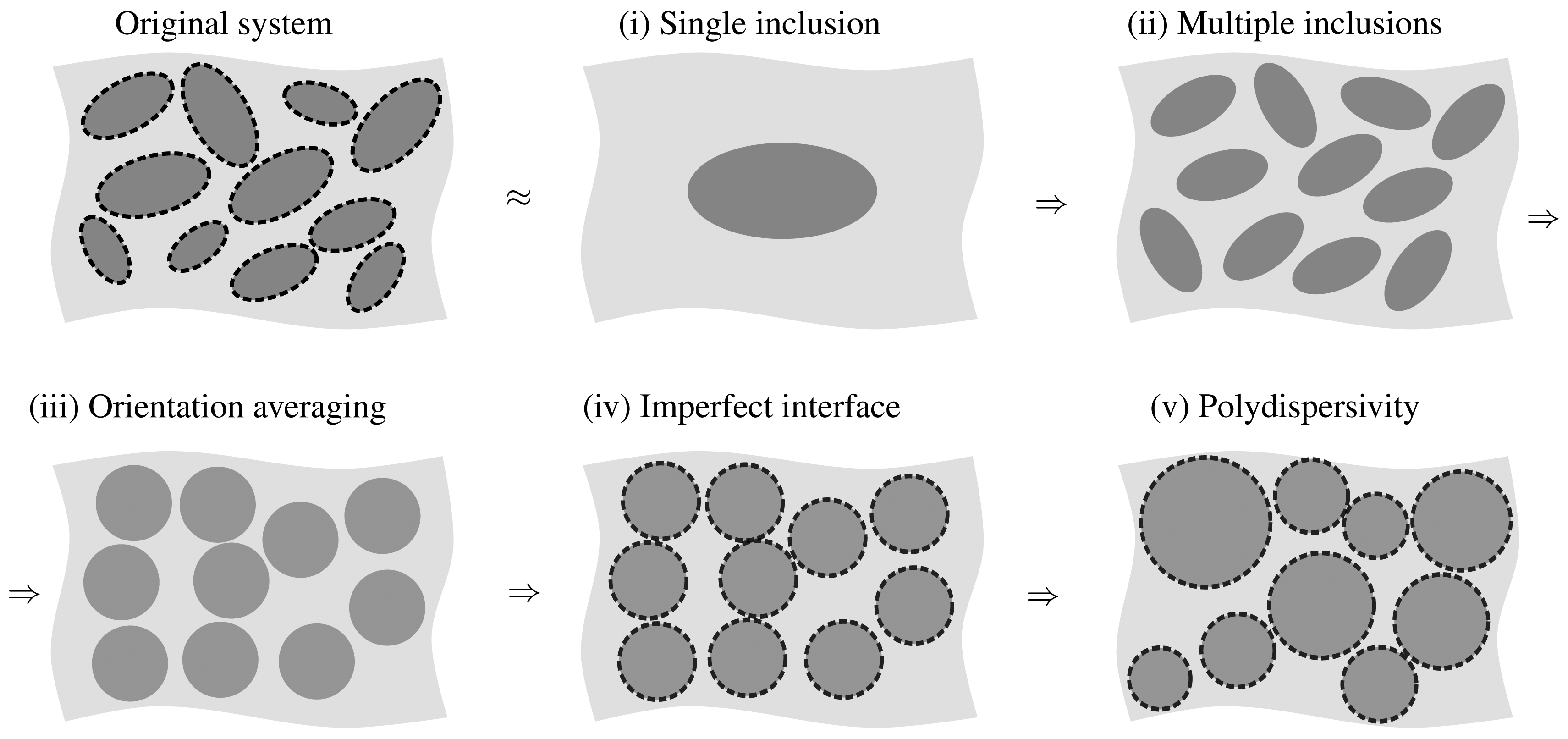
To exploit this result in practical applications of the Mori-Tanaka method to a heat conduction problem, prediction of effective thermal conductivity in particular, we adopt the analysis scheme graphically presented in Figure 3. We start from the assumption of multidisperse system of randomly oriented spheroidal inclusions with possibly imperfect thermal contact (non-zero temperature jump along the interface). We proceed in five consecutive steps to arrive at the desired approximation of multidisperse system of spherical inclusions with perfect interfaces (temperature continuity along the interface).

These steps are mathematically described in Section 2. Section 3 is devoted to both validation and verification of the proposed scheme against available experimental data and finite element simulations performed for several representative statistically isotropic random microstructures. The crucial results and principal recommendations are finally summarized in Section 4.

2. Theoretical Background of the Mori-Tanaka Method

In this section attention is accorded to the essential theoretical details of the Mori-Tanaka method in view of the five steps in Figure 3. In the first step, we consider a single inclusion with perfect interface subject to far-field loading. This step is theoretically elaborated in Section 2.1. Solution of this problem is then employed in Section 2.2 to estimate the overall conductivity of a composite consisting of multiple ellipsoidal inclusions bonded to a matrix phase. The third step addressed in Section 2.3 is reserved for systems with randomly oriented inclusions with a uniform distribution over the hemisphere. Here, a simple orientation averaging argument is shown to demonstrate that the effective conductivity of the system coincides with the conductivity of a system reinforced by spherical inclusions, thermal conductivity of which is appropriately modified. Following [7], an analogous argument is employed in the next step outlined in Section 2.4 to account for imperfect thermal contact along the matrix-inclusion interface. It is shown that in this case the modified conductivity becomes size-dependent. This eventually allows us to extend the scheme to polydisperse systems in Section 2.5.

2.1. Single Inclusion with Perfect Interface

Let us consider an ellipsoidal inclusion Ωⁱ, with semi-axes a₁ ≤ a₂ ≤ a₃ embedded in the matrix domain Ω^m. We attach to the inclusion a Cartesian coordinate system with the origin at the inclusion center and axes aligned with the semi-axes. The distribution of local fields follows from the problem

$$\begin{array}{ccc}\mathit{\text{q}}(\mathit{\text{x}})=-\mathit{\chi }(\mathit{\text{x}})\mathit{\text{h}}(\mathit{\text{x}}),& {\mathbf{\nabla }}^{\mathbf{⊺}}\mathit{\text{q}}(\mathit{\text{x}})=0& \text{for}\mathit{\text{x}}\in {ℝ}^3\end{array}$$

(1)

where q ∈ ℝ³ denotes the heat flux, h ∈ ℝ³ denotes gradient of the temperature θ (i.e., h(x) = ∇θ(x)) and χ designates the 3 × 3 symmetric positive-definite matrix of thermal conductivity given by

$$\mathit{\chi }(\mathit{\text{x}})=\{\begin{array}{cc}{\mathit{\chi }}^{\text{i}}& \text{for}\mathit{\text{x}}\in {\Omega }^i\\ {\mathit{\chi }}^{\text{m}}& \text{otherwise}\end{array}$$

(2)

Equation (1) is completed by the far-field boundary conditions, cf. [5, Equation (14)],

$$\begin{array}{ccc}\theta (\mathit{\text{x}})={\mathit{\text{H}}}^{\mathbf{⊺}}\mathit{\text{x}}& \text{for}& \Vert \mathit{\text{x}}\Vert \to \infty \end{array}$$

(3)

with H ∈ ℝ³ denoting the overall (macroscopic) temperature gradient. Due to linearity of the problem, we can introduce the temperature gradient concentration factor A ∈ ℝ^3×3 in the form

$$\begin{array}{ccc}\mathit{\text{h}}(\mathit{\text{x}})=\mathit{\text{A}}(\mathit{\text{x}})\mathit{\text{H}}& \text{for}& \mathit{\text{x}}\in {ℝ}^3\end{array}$$

(4)

As shown first by Hatta and Taya [11], the concentration factor is constant inside the inclusion and admits the expression

$$\begin{array}{ccc}{\mathit{\text{A}}}^{-1}(\mathit{\text{x}})={({\mathit{\text{A}}}^{\text{i}})}^{-1}=\mathit{\text{I}}-\mathit{\text{S}}{({\mathit{\chi }}^{\text{m}})}^{-1}({\mathit{\chi }}^{\text{m}}-{\mathit{\chi }}^{\text{i}})& \text{for}& \mathit{\text{x}}\in {\Omega }^{\text{i}}\end{array}$$

(5)

where I denotes the unit matrix and S ∈ ℝ^3×3 is the Eshelby-like matrix which depends only on the matrix conductivity χ^m and the ratios of semi-axes lengths β₂ = a₂ : a₁ and β₃ = a₃: a₁, see also Appendix A for additional details. For the spherical inclusion with isotropic conductivity χⁱ = χⁱI embedded in the isotropic matrix with χ^m = χ^mI, Equation (5) simplifies as

$$\begin{array}{ccc}{\mathit{\text{A}}}^{\text{i}}=A_{\text{sph}}^{\text{i}}\mathit{\text{I}}& \text{with}& A_{\text{sph}}^{\text{i}}=\frac{3{\chi }^{\text{m}}}{2{\chi }^{\text{m}}+{\chi }^{\text{i}}}\end{array}$$

(6)

2.2. Multiple Inclusions with Perfect Interface

In the next step, we adopt the results of the previous section to estimate the overall behavior of a composite material consisting of distinct phases r = 0, 1,…, N. The value r = 0 is reserved for the matrix phase Ω^m and the r-th phase (r > 0) corresponds to the ellipsoidal inclusion Ω^(r), characterized by its semi-axes $a_1^{(r)}$, $a_2^{(r)}$ and $a_3^{(r)}$, volume fraction c^(r) and conductivity χ^(r). Following Benveniste's reformulation [12] of the original Mori-Tanaka scheme [13], the interaction among phases is approximated by subjecting each inclusion separately to the mean temperature gradient in the matrix phase H^m in Equation (3). As a result, the temperature gradient inside the r-th phase remains constant and reads

$$\begin{array}{ccc}{\mathit{\text{H}}}^{(r)}={\mathit{\text{T}}}^{(r)}{\mathit{\text{H}}}^{\text{m}}& \text{for}& r=0,1\dots ,N\end{array}$$

(7)

Here,

$${\mathit{\text{H}}}^{(r)}=\frac{1}{\left|{\Omega }^{(r)}\right|}{\mathit{\int }}_{{\Omega }^{(r)}}\mathit{\text{h}}(\mathit{\text{x}})\mathrm{d}\mathit{x}$$

(8)

and T^(r) is the 3 × 3 partial temperature gradient concentration factor of the r-th phase, given by

$${\mathit{\text{T}}}^{(r)}=\{\begin{array}{cc}\mathit{\text{I}}& \text{for}r=0,\hfill \\ {\mathit{\text{R}}}^{(r)}{\mathit{\text{T}}}_{\ell }^{(r)}{({\mathit{\text{R}}}^{(r)})}^{⊺}\hfill & \text{for}r=1,2,\dots ,N\end{array}$$

(9)

where the 3 × 3 rotation matrix R^(r) accounts for the difference in the global and local coordinate systems, see Section 2.3 for additional details, and ${\mathit{\text{T}}}_{\ell }^{(r)}$ equals to Aⁱ in Equation (5) with χⁱ = χ^(r) and S determined from values $a_1^{(r)}$, $a_2^{(r)}$ and $a_3^{(r)}$.

The volume consistency of the overall temperature gradient H and local averages H^(r) requires

$$\mathit{\text{H}}=\sum _{r=0}^N{c}^{(r)}{\mathit{\text{H}}}^{(r)}=\left(\sum _{r=0}^N{c}^{(r)}{\mathit{\text{T}}}^{(r)}\right){\mathit{\text{H}}}^{\text{m}}$$

(10)

Inverting the above equation gives the average temperature gradient in the matrix as

$${\mathit{\text{H}}}^{\text{m}}={\left(\sum _{r=0}^N{c}^{(r)}{\mathit{\text{T}}}^{(r)}\right)}^{-1}\mathit{\text{H}}={\mathit{\text{A}}}^{\text{m}}\mathit{\text{H}}$$

(11)

which, when substituted into Equation (7), yields the explicit expression for the phase temperature gradients in the form

$${\mathit{\text{H}}}^{(r)}={\mathit{\text{T}}}^{(r)}{\left(\sum _{r=0}^N{c}^{(r)}{\mathit{\text{T}}}^{(r)}\right)}^{-1}\mathit{\text{H}}={\mathit{\text{A}}}^{(r)}\mathit{\text{H}}$$

(12)

where A^m, A^(r) are the matrix and inclusion temperature gradient concentration factors, respectively.

As each phase is assumed to be homogeneous, the average heat flux in the r-th phase

$$\begin{array}{cc}{\mathit{\text{Q}}}^{(r)}=\frac{1}{\left|{\Omega }^{(r)}\right|}{\int }_{{\Omega }^{(r)}}\mathit{\text{q}}(\mathit{\text{x}})\mathrm{d}\mathit{x}& \text{for}r=0,1,\dots ,N\end{array}$$

(13)

equals to

$$\begin{array}{cc}{\mathit{\text{Q}}}^{(r)}=-{\mathit{\chi }}^{(r)}{\mathit{\text{H}}}^{(r)}& \text{for}r=0,1,\dots ,N\end{array}$$

(14)

This allows us to express the macroscopic heat flux in the form

$$\mathit{\text{Q}}=\sum _{r=0}^N{c}^{(r)}{\mathit{\text{Q}}}^{(r)}=-\left(\sum _{r=0}^N{c}^{(r)}{\mathit{\chi }}^{(r)}{\mathit{\text{T}}}^{(r)}\right){\left(\sum _{r=0}^N{c}^{(r)}{\mathit{\text{T}}}^{(r)}\right)}^{-1}\mathit{\text{H}}$$

(15)

from which we obtain the effective conductivity Q = −χ^HH in its final form

$${\mathit{\chi }}^{\text{H}}=\left(c^{\text{m}}{\mathit{\chi }}^{\text{m}}+\sum _{r=1}^N{c}^{(r)}{\mathit{\chi }}^{(r)}{\mathit{\text{T}}}^{(r)}\right){\left(c^{\text{m}}\mathit{\text{I}}+\sum _{r=1}^N{c}^{(r)}{\mathit{\text{T}}}^{(r)}\right)}^{-1}$$

(16)

Finally, assuming that the composite consists of isotropic matrix with conductivity χ^m and spherical isotropic inclusions with conductivities χ^(r), Equation (16) becomes χ^H = χ^HI, with

$$\begin{array}{ccc}{\chi }^{\text{H}}=\frac{c^{\text{m}}{\chi }^{\text{m}}+\text{∑}_{r=1}^N{c}^{(r)}{\chi }^{(r)}{T}_{\text{sph}}^{(r)}}{c^{\text{m}}+\text{∑}_{r=1}^N{c}^{(r)}{T}_{\text{sph}}^{(r)}}& \text{and}& T_{\text{sph}}^{(r)}=\frac{3{\chi }^{\text{m}}}{2{\chi }^{\text{m}}+{\chi }^{(r)}}\end{array}$$

(17)

2.3. Orientation Averaging

We are now in a position to provide estimates of the effective thermal conductivity for composites with M (with M ≪ N) inclusion classes indexed by s = 1, 2,…, M. Each class is characterized by a single Eshelby-like matrix S in Equation (5) and represents the reference ellipsoidal inclusion randomly oriented over the unit hemisphere with an independent uniform distribution of orientation angles.

To this goal, consider a quantity X_ℓ ∈ ℝ^3×3, expressed in a local coordinate system aligned with a certain reference inclusion. Its form in the global coordinate system follows from

$$\mathit{\text{X}}(\phi ,\varphi ,\psi )=\mathit{\text{R}}(\phi ,\varphi ,\psi ){\mathit{\text{X}}}_{\ell }{\mathit{\text{R}}}^{⊺}(\phi ,\varphi ,\psi )$$

(18)

where φ, ϕ and ψ denote the Euler angles(Note that so-called “x₂ convention” is used, in which a conversion into a new coordinates system follows three consecutive steps. First, the rotation of angle φ around the original X₃ axis is done. Then, the rotation of angle ϕ around the new x₂ axis is followed by the rotation of angle ψ around the new x₃ axis to finish the conversion.) and the transformation matrix R is provided by

$$\mathit{\text{R}}(\phi ,\varphi ,\psi )=\left[\begin{array}{rrr}\hfill cos\psi & \hfill -sin\psi & \hfill 0\\ \hfill sin\psi & \hfill cos\psi & \hfill 0\\ \hfill 0& \hfill 0& \hfill 1\end{array}\right]\left[\begin{array}{rrr}\hfill cos\varphi & \hfill 0& \hfill -sin\varphi \\ \hfill 0& \hfill 1& \hfill 0\\ \hfill sin\varphi & \hfill 0& \hfill cos\varphi \end{array}\right]\left[\begin{array}{rrr}\hfill cos\phi & \hfill -sin\phi & \hfill 0\\ \hfill sin\phi & \hfill cos\phi & \hfill 0\\ \hfill 0& \hfill 0& \hfill 1\end{array}\right]$$

(19)

The orientation average of X is denoted by double angular brackets

$$\langle \langle \mathit{\text{X}}\rangle \rangle =\frac{1}{8{\pi }^2}{\mathit{\int }}_0^{2\pi }{\mathit{\int }}_0^{\pi }{\mathit{\int }}_0^{2\pi }\mathit{\text{X}}(\phi ,\varphi ,\psi )sin\varphi \text{d}\phi \text{d}\varphi \text{d}\psi$$

Straightforward calculation, presented in [14, Appendix A.2.3], reveals that the orientation averaging of an arbitrary X_ℓ ∈ ℝ^3×3 yields

$$\begin{array}{ccc}\langle \langle \mathit{\text{X}}\rangle \rangle =\langle \langle X\rangle \rangle \text{I}& \text{with}& \langle \langle X\rangle \rangle =\frac{1}{3}\sum _{i=1}^3{(X_{\ell })}_{ii}\end{array}$$

(21)

Repeating the steps of the previous section with partial temperature gradient concentration factors replaced with their orientation averages, we obtain, after some manipulations presented in [15, Section B], the scalar homogenized conductivity in the form

$${\chi }^{\text{H}}=\frac{c^{\text{m}}{\chi }^{\text{m}}+\text{∑}_{s=1}^M{c}^{(s)}\langle \langle {\chi }^{(s)}{T}^{(s)}\rangle \rangle }{c^{\text{m}}+\text{∑}_{s=1}^M{c}^{(s)}\langle \langle T^{(s)}\rangle \rangle }$$

(22)

Therefore, it follows from the comparison of Equation (22) with Equation (17) that the system of randomly oriented inclusions embedded in an isotropic matrix is indistinguishable, from the point of view of homogenized conductivity, from the system of spherical inclusions with an apparent conductivity

$${\tilde{\chi }}^{(s)}=\frac{3{\chi }^{\text{m}}}{\langle \langle T^{(s)}\rangle \rangle }-2{\chi }^{\text{m}}$$

(23)

which yields

$$\begin{array}{ccc}{\chi }^{\text{H}}=\frac{c^{\text{m}}{\chi }^{\text{m}}+\text{∑}_{s=1}^M{c}^{(s)}{\tilde{\chi }}^{(s)}{\tilde{T}}_{\text{sph}}^{(s)}}{c^{\text{m}}+\text{∑}_{s=1}^M{c}^{(s)}{\tilde{T}}_{\text{sph}}^{(s)}}& \text{with}& {\tilde{T}}_{\text{sph}}^{(s)}=\frac{3{\chi }^{\text{m}}}{2{\chi }^{\text{m}}+{\tilde{\chi }}^{(s)}}\end{array}$$

(24)

2.4. Imperfect Interface

The presence of imperfect thermal contact at the matrix-inclusion interface ∂Ωⁱ results in temperature jump 〚θ〛, the magnitude of which is provided by Newton's law, e.g., [16, Section 1.3]

$$\begin{array}{cc}{\mathit{\text{n}}}^{⊺}(\mathit{\text{x}})\mathit{\text{q}}(\mathit{\text{x}})=k(\mathit{\text{x}})〚\theta (\text{x})〛& \text{for}\mathit{\text{x}}\in \partial {\Omega }^{\text{i}}\end{array}$$

(25)

where k denotes the interfacial conductance (with k → ∞ corresponding to perfect interface and k = 0 to ideal insulation) and n denotes the normal vector at the interface oriented outside the inclusion. This relation, together with Equations (1)–(3), defines the single inclusion problem accounting for the presence of imperfect interface. Its solution is, however, substantially more involved as the temperature gradient inside an ellipsoidal inclusion becomes position-dependent; the concentration factor is then available only in the form of complicated infinite series expansion for spheroidal inclusions [5] or ellipsoidal coated inclusions [10]. Nevertheless, when restricting the attention to spherical inclusion of radius a, it can be shown that the temperature gradient within inclusion recovers the constant value and the concentration factor becomes [5]

$$\begin{array}{ccc}{\widehat{A}}_{\text{sph}}({\chi }^{\text{i}},k,a)=\frac{3{\chi }^{\text{m}}}{2{\chi }^{\text{m}}+{\widehat{\chi }}^{\text{i}}({\chi }^{\text{i}},k,a)}& \text{where}& {\widehat{\chi }}^{\text{i}}({\chi }^{\text{i}},k,a)\end{array}={\chi }^{\text{i}}\frac{ak}{ak+{\chi }^{\text{i}}}$$

(26)

see also Appendix B for simple derivation of this result. Hence, analogously to the previous section, the interfacial effect can be modeled by replacing the “true” conductivity χⁱ by the size-dependent apparent value ${\widehat{\chi }}^{\text{i}}$ provided by Equation (26). Assuming in addition that each class of inclusions is characterized by identical semi-axes lengths $a_1^{(s)}$, $a_2^{(s)}$ and $a_3^{(s)}$ and interfacial conductance k^(s), we propose to extend the relation (24) into the form, cf. [7, Section 2]

$$\begin{array}{ccc}{\chi }^{\text{H}}=\frac{c^{\text{m}}{\chi }^{\text{m}}+\text{∑}_{s=1}^M{c}^{(s)}{\widehat{\chi }}^{(s)}{\widehat{T}}_{\text{sph}}^{(s)}}{c^{\text{m}}+\text{∑}_{s=1}^M{c}^{(s)}{\widehat{T}}_{\text{sph}}^{(s)}},& {\tilde{T}}_{\text{sph}}^{(s)}=\frac{3{\chi }^{\text{m}}}{2{\chi }^{\text{m}}+{\widehat{\chi }}^{(s)}},& {\widehat{\chi }}^{(s)}={\widehat{\chi }}^{(s)}\frac{a^{(s)}{k}^{(s)}}{a^{(s)}{k}^{(s)}+{\widehat{\chi }}^{(s)}}\end{array}$$

(27)

with $a^{(s)}=\sqrt[3]{a_1^{(s)}{a}_2^{(s)}{a}_3^{(s)}}$and the apparent conductivity ${\tilde{\chi }}^{(s)}$ given by Equation (23).

2.5. Polydisperse Systems

Even though Equation (27) is applicable to very general material systems, in practice we typically assume single inclusion family, with the particle size distribution characterized by a probability density function p(a) satisfying

$$\begin{array}{cc}p(a)\ge 0\text{for}-\infty <a<\infty ,& {\mathit{\int }}_{-\infty }^{\infty }p(a)\text{d}a=1\end{array}$$

(28)

In this context, the effective conductivity finally becomes

$${\chi }^{\text{H}}=\frac{c^{\text{m}}{\chi }^{\text{m}}+c^{(1)}\left\{{\widehat{\chi }}^{(1)}{\widehat{T}}_{\text{sph}}^{(1)}\right\}}{c^{\text{m}}+c^{(1)}\left\{{\widehat{T}}_{\text{sph}}^{(1)}\right\}}$$

(29)

where, for an arbitrary function g(a), {g} denotes its expected value given by

$$\{g\}={\int }_{-\infty }^{\infty }g(a)p(a)\text{d}a$$

(30)

Following [7,17], the log-normal distribution with the probability density function

$$\begin{array}{cc}p(a)=\frac{1}{\sqrt{2\pi }a\sigma }exp\left(-{\left[\frac{\text{In}(a)-\mu }{\sqrt{2}\sigma }\right]}^2\right),& a>0\end{array}$$

(31)

will be employed to characterize the materials' polydispersity. The parameters μ and σ are provided by [7, Equation (17)]

$$\begin{array}{ccc}\mu =\text{In}(a_{50}),& \sigma =\frac{1}{1.2816}\text{In}\left(\frac{S+\sqrt{S^2+4}}{4}\right),& S=\frac{a_{90}-a_{10}}{a_{50}}\end{array}$$

(32)

where a_x denotes the x-th percentile of the particle radii and S is the span of the size distribution.

3. Mori-Tanaka Estimates: Example Results

3.1. Validation Against Available Experimental Data

Two particular examples of real engineering materials are examined in this section to show applicability of Equation (27) and its extension for polydisperse distribution of heterogeneities, Equation (29), even when disregarding their actual shape and simply accepting a spherical representation of the inclusions in the Mori-Tanaka predictions. The results provided by these two equations are corroborated by available experimental data.

3.1.1. Random Dispersion of Copper Particles in the Epoxy Matrix

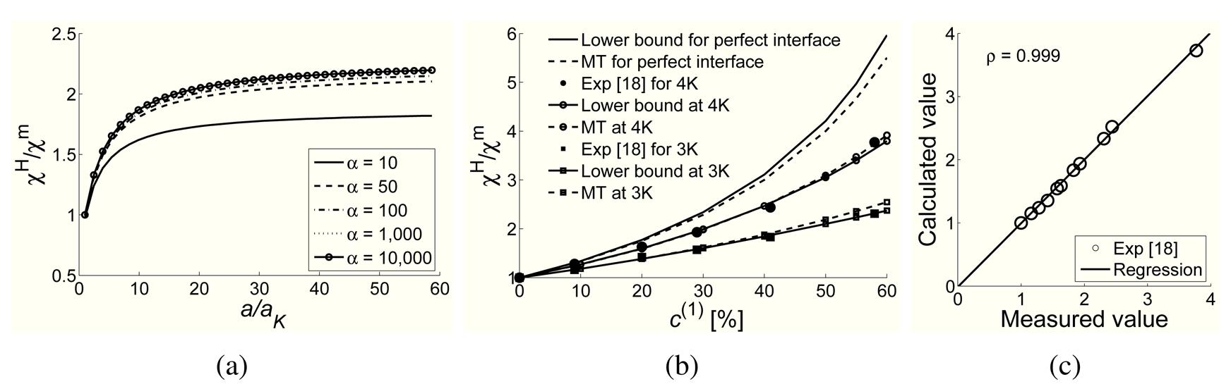
In this first example we compare the single-phase Mori-Tanaka predictions with the experimental results of de Araujo and Rosenberg [18], who measured the effective thermal conductivities of systems consisting of randomly dispersed metal particles in the epoxy matrix, and obtained several values of the interfacial resistance due to acoustic mismatch at the particle-matrix interface, particularly for low temperatures below 20 K. To enhance the credibility of the Mori-Tanaka predictions we focus on one particular system made from epoxy resin filled with copper particles also examined in [8] in view of the three-point lower bound assuming a random array of superconducting hard spheres (i.e., χ⁽¹⁾ → ∞). It has been shown, see [18,19], that for metal-filled composites with ratio α = χ⁽¹⁾/χ^m > 10² the macroscopic conductivity does not depend on the thermal conductivity of the metallic filler, but only on its volume fraction together with the properties of matrix and matrix-particle interface. This becomes evident when rewriting Equation (27) in terms of α

$$\frac{{\chi }^{\text{H}}}{{\chi }^{\text{m}}}=1+\frac{3c^{(1)}[\alpha -(1+R)]}{c^{\text{m}}[\alpha +2(1+R)]+3c^{(1)}(1+R)}$$

(33)

where we introduced the dimensionless quantity R adopted in [8]

$$R=\frac{{\chi }^{(1)}}{ka}=\frac{\alpha {\chi }^{\text{m}}}{ka}$$

(34)

where a is the sphere radius. It follows from Equation (33) that for the inclusion size equal to the Kapitza radius [20]

$$a_{\text{K}}=\frac{\alpha }{\alpha -1}\frac{{\chi }^{\text{m}}}{k}\approx \frac{{\chi }^{\text{m}}}{k}$$

(35)

the effective conductivity equals to that of the matrix, thus the effect of inclusions becomes completely shielded by the interface. For a < a_K, the overall properties are dominated by interfaces and the effective conductivity decreases with increasing c⁽¹⁾ even when α > 1. For a > a_K, the bulk properties of phases become dominant; see also [20] for further discussion.

In addition to experimental measurements, we also present a comparison with the Torquato-Rintoul three-point lower bound in resistance case derived in [8, Equation (8)], evaluated for the statistical parameter ζ(c⁽¹⁾) given for the model of impenetrable spheres in [21, Table II (simulations)]. Note that the interfacial properties can be estimated by measuring the ratio of temperature jump to the applied heat flux across a thin bi-material layer, by acoustic mismatch model [4] or, indirectly, from an inverse approach as discussed below. The results are presented for two different temperatures θ = 4 K (a = 14.8 a_K) and θ = 3 K (a = 4.93 a_K).

The influence of parameter α together with expected particle size dependence, now hidden in parameter R through Equation (34), is evident from Figure 4(a) plotted for θ = 4K (a_K = 3.38 μm). Clearly, the Mori-Tanaka predictions confirm negligible influence of χ⁽¹⁾ observed for particulate composites with χ⁽¹⁾ ≫ χ^m (α > 10²) as well as decreasing trend for χ^H with decreasing particle size caused by imperfect thermal contact. Figure 4(b) then displays evolution of normalized effective thermal conductivity as a function of volume fraction of copper particles. Predictive capability of the Mori-Tanaka method is supported here by a very good agreement with both experimental measurements and the Torquato-Rintoul bounds [8]. Finally, Figure 4(c) shows correlation between theoretical (MT predictions) and experimental results. The solid line was derived by linear regression of measured and calculated effective conductivities using the least square method. Another indication of the quality of numerical predictions can be presented in the form of Pearson's correlation coefficient written as

$$\rho =\frac{n\langle xy\rangle -\langle x\rangle \langle y\rangle }{\sqrt{n\langle x^2\rangle -{\langle x\rangle }^2}\sqrt{n\langle y^2\rangle -{\langle y\rangle }^2}},$$

(36)

where $\langle a\rangle ={\sum }_{i=1}^n{a}_i$, n is the number of measurements, x stands for the experimental and y for the corresponding theoretical values. Note that for ρ = 1 the correspondence is exact. In this case the correlation coefficient equals to 0.999, suggesting almost perfect match between measured and predicted values, also evident from graphical presentation.

3.1.2. Al/SiC Composite

In [4] the authors studied the effect of imperfect thermal contact on the macroscopic response of Al/SiC porous composites. The paper presents the results of a thorough experimental investigation and the traces of an inverse approach in material mechanics for inferring material properties of unknown components of the composite by matching numerical and experimental results. This approach was first exploited to derive the matrix thermal conductivity from known electrical conductivity of the composite. Next, the Hasselman and Johnson model [3] was employed under the premise of random distribution of spherical particles of identical size to estimate the particle thermal conductivity and interfacial thermal conductance for pore-free specimens and subsequently utilized in the two-step application of the Hasselman-Johnson model to address the influence of pores. Note that the material data used in these predictions can be thought as optimal with respect to the adopted Hasselman-Johnson model.

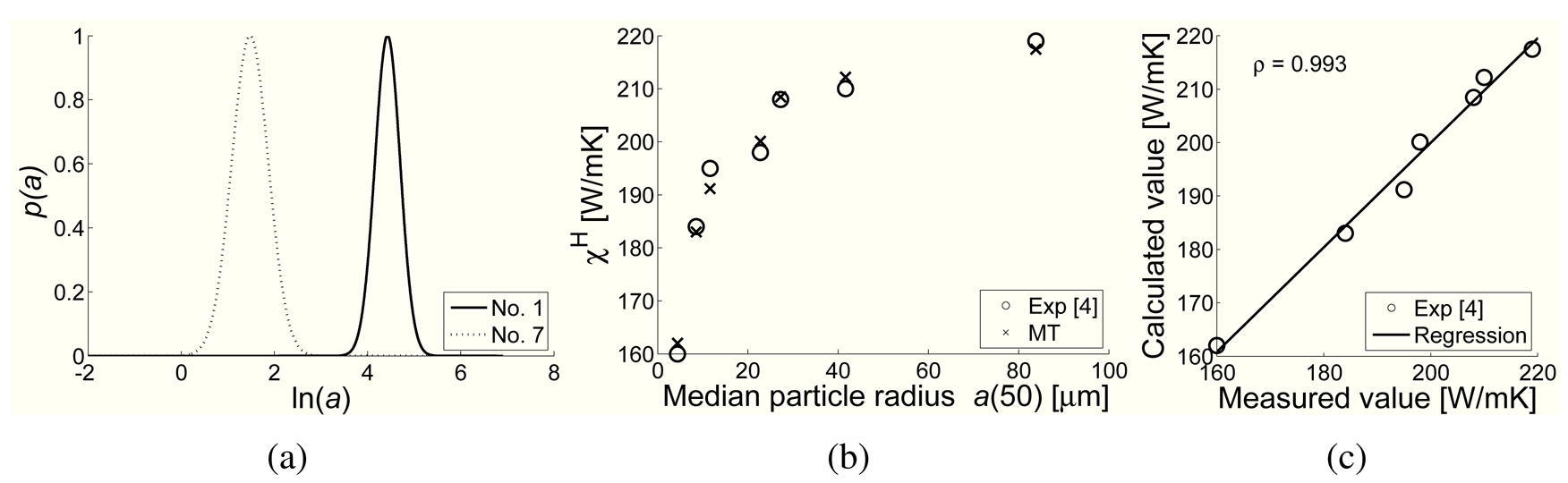
Hereinafter, we compare the results presented in [4] for seven specimens with pore-free matrix. In addition, we take advantage of available characteristics of the SiC particles, the span S and the 50th percentile a₅₀, to extend the analysis to polydisperse systems as presented in Section 2.5. The input material data are listed in

Table 1. Material properties [4].

Al matrix	SiC particles	Interface
[Wm−1K−1]		[Wm−2K−1]
187	252.5	72.5 × 106

.

The Mori-Tanaka predictions stored in

Table 2. Characteristics of SiC particles (cf. [4, Table 1]), and comparison of effective thermal conductivity χ^H [Wm⁻¹K⁻¹] between experimental measurements [4] and MT predictions (29).

Sample No.	Radius [μm]			SiC vol.	Results
	a10	a90	S		Exp.	MT
1	55	114.5	0.71	0.58	219	217.8
2	23	65.5	1.02	0.58	210	212.3
3	19.5	37.5	0.66	0.60	208	208.5
4	11.5	25	0.79	0.59	198	199.9
5	7	17	0.86	0.58	195	190.8
6	5	12	0.82	0.55	184	182.5
7	2.4	7	1.05	0.53	160	161.3

were provided by Equation (29). The integral (30) was evaluated such that the entire interval was split into 1,000 segments, thus considering 1,000 different particle sizes of spherical shape. Within each segment s the probability function p(a) was approximated by a straight line and the volume fraction c⁽¹⁾ of a given set of particles, given by the segment area, was then associated in a logarithmic way with the mean radius a⁽¹⁾of this set of particles. Standard trapezoidal integration rule was then used to sum over all 1,000 segments. Examples of probability distribution functions for specimens No. 1 and 7 are plotted in Figure 5.

Graphical representation of the results is further seen in Figure 5(b,c) confirming the sensitivity of the effective thermal conductivity to the mean particle size distribution. Note that individual points in Figure 5(b) correspond to slightly different volume fraction, see Table 2.

Almost negligible deviation from experimental results measured as

$$E=\sqrt{\frac{\text{∑}_i{({\chi }^{exp}-{\chi }^{\text{MT}})}^2}{\text{∑}_i{({\chi }^{\text{MT}})}^2}}=1.1\%$$

is, however, not surprising owing to the used material parameters, which were not measured but rather fitted to a micromechanical model. Even when comparing the Pearson correlation coefficients, 0.98 for the Hasselman-Johnson model and 0.993 for polydisperse MT model, the improvement when accounting for more accurate representation of particle size distribution is marginal. This can be explained by a very small variance associated with adopted distributions, recall Figure 5(a). Nevertheless, it is fair to point out that unlike the Hasselman-Johnson model the Mori-Tanaka approach is not limited to spherical particles providing the transformations given by Equations (24) and (27) are admissible. The influence of shape of particles on the macroscopic response has been put forward, e.g., by Jäckel in [19], and is numerically investigated in the next section suggesting increasing thermal conductivity of the composite with transition from spherical to needle-like particles. The trend is also observed experimentally [18,19].

3.2. Verification Against Finite Element Simulations

It has been argued in the previous sections that even very limited information about microstructure amounted to phase properties and corresponding volume fractions might be sufficient to provide a reasonable estimate of macroscopic response of various engineering material systems generally classified as being macroscopically isotropic. This naturally invites the assumption of spherical representation of otherwise irregular heterogeneities. Although supported by several practical examples discussed in the previous section, we should expect and even identify, at least qualitatively, limitations to such perception. In doing so, this section presents numerical investigation of some specific issues such as the influence of shape and size of inclusions or mismatch of phase material properties on the predicted macroscopic response.

All numerical results reported bellow are obtained in the two-dimensional setting, hence the arguments presented in Section 2 need to be translated to the planar case. In particular, inclusions are modeled as elliptic cylinders of aspect ratio β₂ = a₂/a₁ with a₃ → ∞. The corresponding Eshelby-like tensor is given by Equation (43), which leads to the two-dimensional thermal concentration factor for circular inclusion in the form

$$\begin{array}{ccc}{\mathit{\text{A}}}^{\text{i}}=A_{\text{cir}}^{\text{i}}{\mathit{\text{I}}}_{(2\times 2)}& \text{with}& A_{\text{cir}}^{\text{i}}=\frac{2{\chi }^{\text{m}}}{{\chi }^{\text{m}}+{\chi }^{\text{i}}}\end{array}$$

(37)

The apparent conductivity due to random orientation is provided by

$${\tilde{\chi }}^{(s)}=\frac{2{\chi }^{\text{m}}}{{\langle \langle T^{(s)}\rangle \rangle }_{2\text{D}}}-{\chi }^{\text{m}}$$

(39)

where 《●》_2D stands for the orientation averaging for the uniform distribution of the Euler angle ϕ. Finally note that the apparent conductivity due to imperfect interface is provided by the same relation as in the three-dimensional setting, compare Equation (26) with Equation (51).

Three particular representatives, generated such as to approximately resemble the real microstructures in Figure 1, appear in Figure 6. To comply with general assumptions put forward in the previous sections, we consider locally isotropic phases with variable contrast of material properties. Additionally, we assume the above microstructures being periodic and adopt the classical first-order homogenization strategy, see e.g., [22,23], to provide estimates of the macroscopic response. The results are plotted in Figure 7.

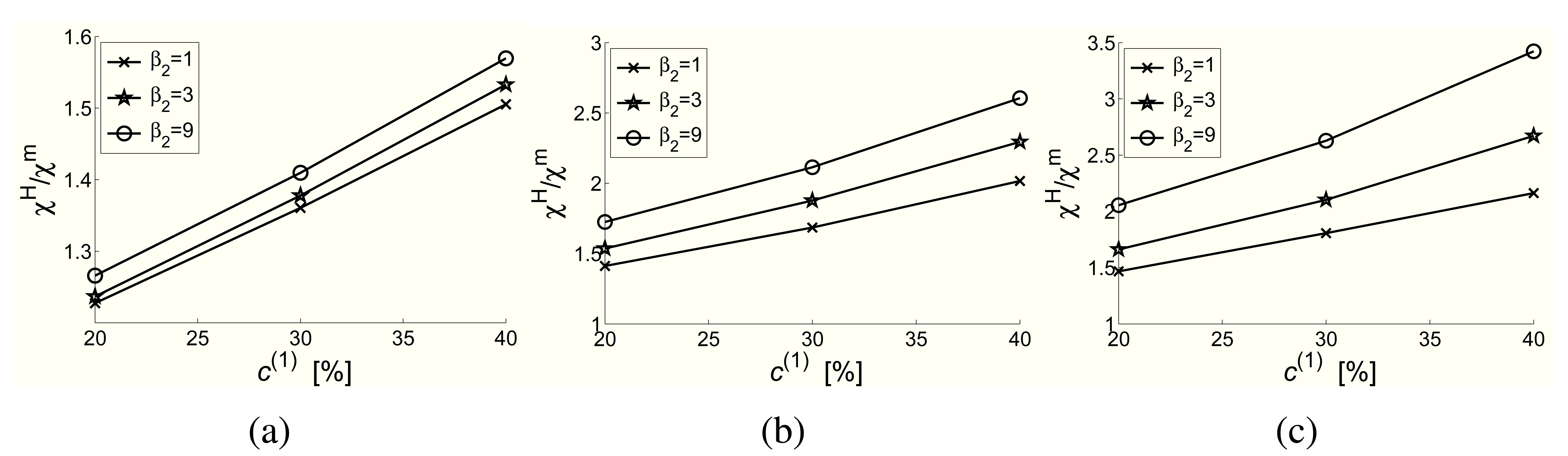
These results clearly indicate not only the influence of the shape of inclusions on the macroscopic response but also a strong dependence of these predictions on the contrast of material properties of individual phases. Thus drawing from the plots presented in Figure 7(a) one may suggest that the proposed circular representation of generally non-circular heterogeneities is still acceptable when their shapes only moderately deviate from a circle and when the mismatch of phase properties is not too severe, which certainly is the case of a number of real materials as demonstrated in the previous section. This expectation is quite important particularly when dealing with imperfect thermal contact in which case only spherical and circular inclusions can be easily handled analytically.

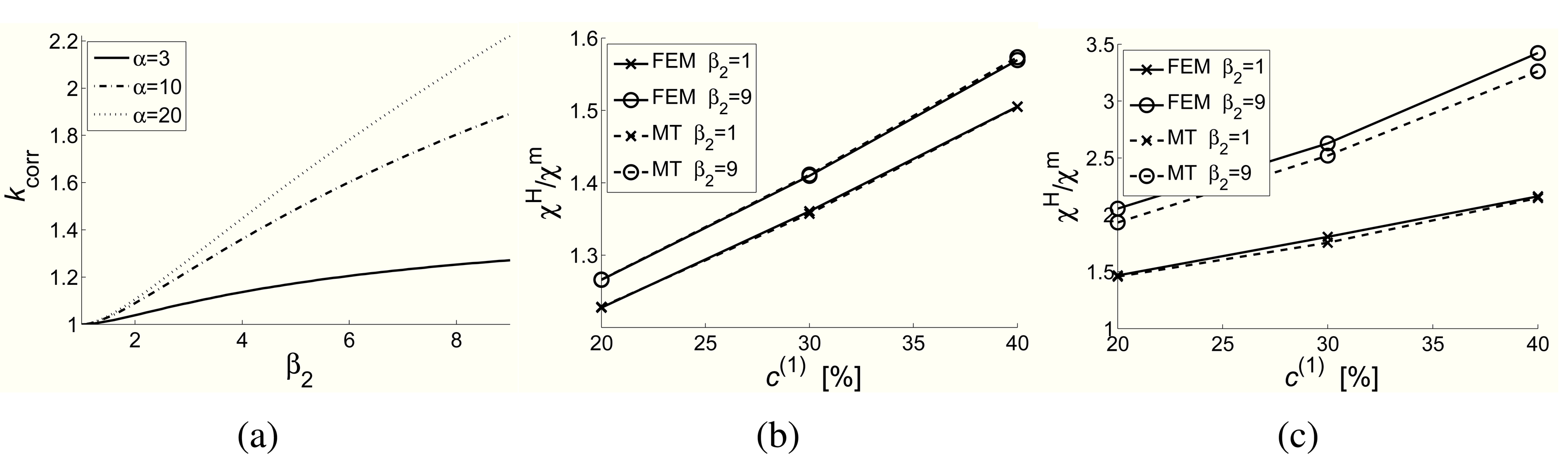
If the circular approximation of heterogeneities is no longer acceptable or the contrast of phase properties is excessive, one needs to look for more details about microstructure. In such a case, even two-dimensional images of real systems, at present almost standard input for any material based analysis, may play an important role in assessing better approximations of shapes, say elliptical, of these heterogeneities, see e.g., [24]. Then, being given the elliptical shape of the inclusion allows us to appropriately modify its material data, recall Equation (38), and define a certain indicator of the real microstructure k_corr, e.g., as a ratio of the modified and original conductivity of the inclusion

$$k_{\text{corr}}=\frac{{\tilde{\chi }}^{(1)}}{{\chi }^{(1)}}$$

(39)

Variation of this parameter as a function of the shape of inclusion is seen in Figure 8(a), further confirming quite strong influence of the phase properties' mismatch (Note that the parameter k_corr is determined for two dimensional systems and thus is not applicable to ellipsoidal inclusions of the same aspect ratio.). The modified conductivity when introduced successively into Equations (37) and (24) then renders the estimate of effective conductivity almost identical to actual microstructure with non-circular inclusions as evident from plots in Figure 8(b,c). Note that only the first and the third microstructure in Figure 6 were examined to first confirm that the Mori-Tanaka method is indeed well suited for statistically isotropic random microstructures and second to promote applicability of this simple transformation from elliptical to circular representations even for shapes markedly distinct from circles. Small but evident deviation of the results observed in Figure 6 for the third needle-like microstructure and large mismatch of conductivities of the inclusion and matrix equal to 20 can be attributed to the finite size, although infinite in the sense of periodicity, of the representative model not large enough to yield statistically isotropic microstructure.

The second set of numerical simulations addresses the theoretically derived dependence of macroscopic predictions on the size of inclusions in cases with imperfect interfaces generating jumps in the local temperature field. For simplicity, we limit our attention to statistically isotropic distributions of circular cylinders with a radius varying from sample to sample. Three such microstructures are shown in Figure 9. Note that the same volume fraction and the same number of inclusions was maintained in all simulations. Zero thickness interface elements were introduced to account for imperfect thermal contact.

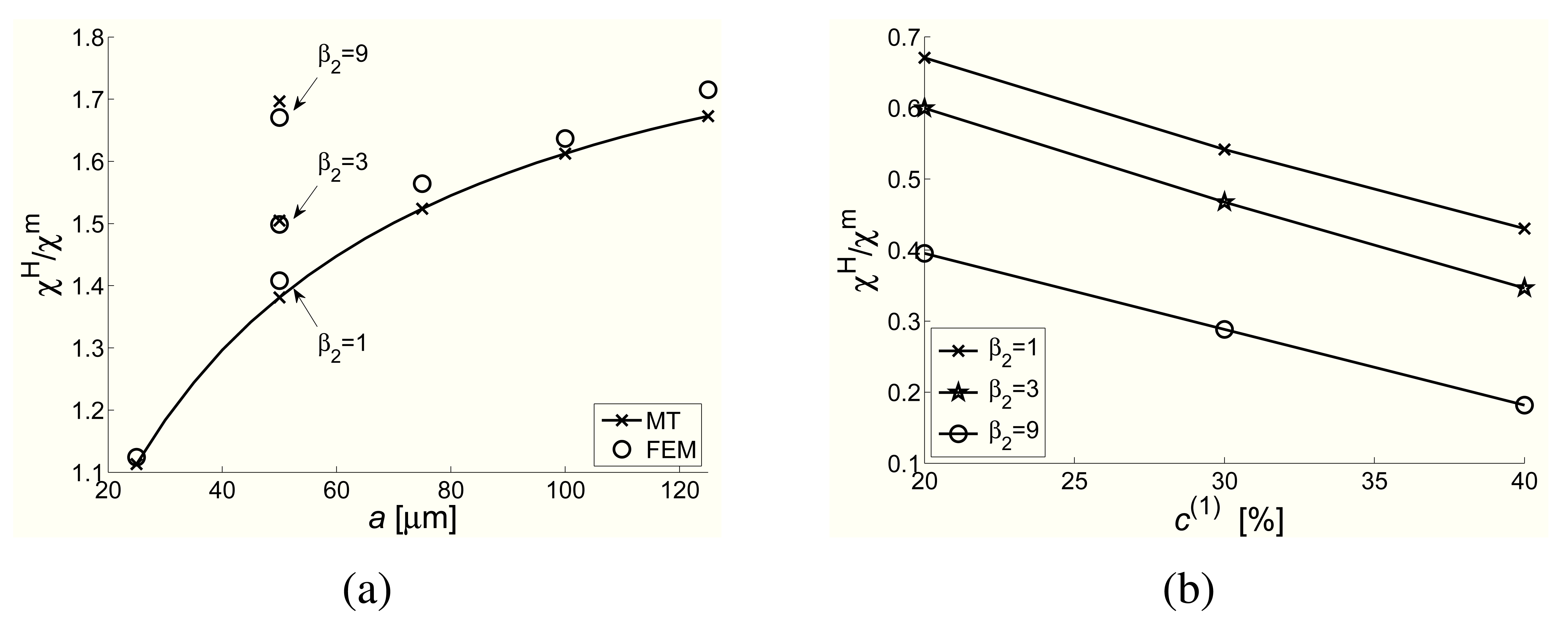
The relevant results appear in Figure 10(a). Both the results found from finite element simulations and corresponding Mori-Tanaka predictions are displayed to clearly identify the mentioned size dependence. Proper modifications in the sense of Equation (38) now become even more important as indicated by the results generated for elliptical microstructures from Figure 6 with cross-sectional area equal to the area of the circle. These are indicated by x-symbol and the ratio of semi-axes of the corresponding elliptical cylinder. The Mori-Tanaka estimates found from the application of Equations (26) and (38) and reasonably close, further supporting the proposed approach for the modeling of real materials with an imperfect thermal contact. Intuitively, it can be expected that the value of interfacial conductance k may also show some effect as to the estimates of effective conductivities for non-circular inclusions. This notion is supported by the results presented in Figure 10(b) showing variation of effective conductivity of an isotropic matrix weakened by voids with a very low conductivity. Clearly, the influence of shape of the inclusions is quite pronounced.

4. Conclusions

The Mori-Tanaka micromechanical model has been often the primary choice among engineers to provide quick estimates of the macroscopic response of generally random composites. Motivated by early theoretical as well as experimental works on this subject, the Mori-Tanaka method was examined here in the light of the solution of a linear steady state heat conduction problem allowing us to estimate the effective thermal conductivity of a variety of real engineering materials experiencing an imperfect thermal contact along the constituents interfaces.

Adhering to the only limitation, an assumption of macroscopically isotropic composite, it was shown that the method originally proposed by Böhm and Nogales [7] for a spherical representation of particles still applies even to non-spherical particles, provided their shape can be suitably quantified, e.g., by an ellipsoidal inclusion. In this particular case the Mori-Tanaka predictions were partially corroborated by two-dimensional numerical simulations confirming experimentally observed considerable sensitivity of macroscopic conductivities to the shape of particles.

The fact that for composites with imperfect thermal contact the macroscopic predictions depend on particle size can be effectively handled by introducing the particle size probability density function directly into the Mori-Tanaka estimates. Although not confirmed for material systems studied in the paper, this may considerably improve final predictions especially for grading curves showing significant standard deviation of particle sizes from its mean value. This is particularly appealing, since grading curves are one of the few information supplied by the manufacturer.

To conclude, it is interesting to point out that there exist many material systems that can be handled very effectively with simple micromechanical models with no need for laborious finite element simulations of certain representative volumes of real microstructures.

A. Eshelby-Like Tensor

The Eshelby-like tensor for the solution of thermal conductivity problem was introduced by Hatta and Taya in [11]. For an ellipsoidal inclusion with semi-axes a₁, a₂, a₃ found in an isotropic matrix it receives the form

$$S_{ij}=\frac{a_1{a}_2{a}_3}{4}\frac{\partial }{\partial x_i\partial x_j}{\mathit{\int }}_0^{\infty }\left(\frac{x_1^2}{a_1^2+s}+\frac{x_2^2}{a_2^2+s}+\frac{x_3^2}{a_3^2+s}\right)\frac{1}{\Delta s}\text{d}s$$

(40)

$$\Delta s=\sqrt{(a_1^2+s)(a_2^2+s)(a_3^2+s)}$$

(41)

Closed form solutions of integral (40) for some special cases of ellipsoidal shapes of the inclusion can be found in [11]. For a general ellipsoid the solution was introduced by Chen and Yang in [25]. For circular and spherical shapes needed in the present study the S tensor reads

• Sphere (a₁ = a₂ = a₃)

  $$\begin{array}{rrrrr}\hfill S_{11}=S_{22}=S_{33}=\frac{1}{3}& \hfill \text{and}& \hfill S_{ij}=0& \hfill \text{for}& \hfill i\ne j\end{array}$$

  (42)

• Elliptic cylinder (a₃ → ∞)

  $$\begin{array}{rrrrrrr}\hfill S_{11}=\frac{a_2}{a_1+a_2},& \hfill S_{22}=\frac{a_1}{a_1+a_2},& \hfill S_{33}=0& \hfill \text{and}& \hfill S_{ij}=0& \hfill \text{for}& \hfill i\ne j\end{array}$$

  (43)

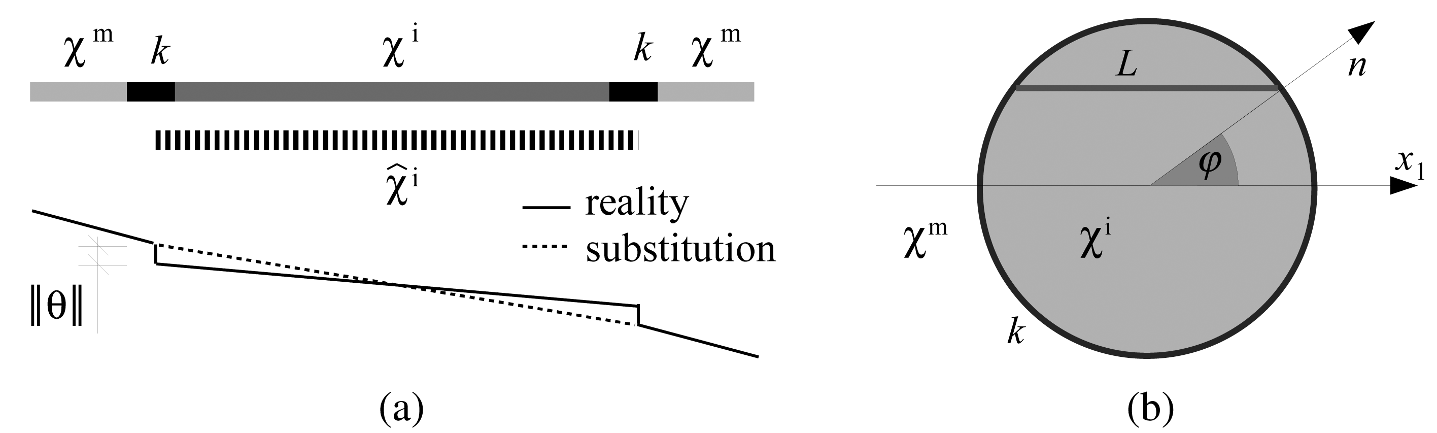
B. Single Spherical Homogeneity with Imperfect Interface

This section outlines derivation of the replacement conductivity ${\widehat{\chi }}^{\text{i}}$ and the concentration factor ${\widehat{A}}_{\text{sph}}$ introduced in Equation (26). Its two dimensional format is used in numerical calculations and presented in Section 3.2 as well. It is shown that both 2D and 3D concentration factors can be recovered from the solution of a 1D problem using a simple geometrical argument.

To that end, consider one-dimensional heat conduction problem depicted in Figure 11(a). Assuming imperfect thermal contact, the temperature drop across an infinitely thin interface layer is given by Equation (25). The local temperature gradient for perfect interface between a solitary inclusion embedded into an infinite matrix follows from Equation (4)

$$H^{\text{i}}={\mathit{\text{A}}}^{\text{i}}H=\frac{{\chi }^{\text{m}}}{{\chi }^{\text{i}}}H$$

(44)

To arrive at similar format of Equation (44) for imperfect contact, we imagine the interface temperature jump being smeared over the inclusion. Since the heat flux Q associated with the macroscopic temperature gradient H is constant throughout the composite, we obtain the total temperature change in the substitute inclusion in the form

$$\Delta \widehat{{\theta }^{\text{i}}}+\Delta {\theta }^{\text{i}}+2〚\theta 〛=-Q\left(\frac{L}{{\chi }^{\text{i}}}+\frac{2}{k}\right)$$

(45)

where L stands for the inclusion length. Next, defining the local temperature gradient in the substitute inclusion as $H^{\text{i}}=\Delta \widehat{{\theta }^{\text{i}}}/L$ yields the local constitutive law in terms of the replacement conductivity ${\widehat{\chi }}^{\text{i}}$

$$Q=-{\widehat{\chi }}^{\text{i}}{H}^{\text{i}}=-{\widehat{\chi }}^{\text{i}}\frac{\Delta \widehat{{\theta }^{\text{i}}}}{L}=-\frac{{\widehat{\chi }}^{\text{i}}}{L}\left[-Q\left(\frac{L}{{\chi }^{\text{i}}}+\frac{2}{k}\right)\right]$$

(46)

so that

$${\widehat{\chi }}^{\text{i}}={\chi }^{\text{i}}\frac{Lk}{Lk+2{\chi }^{\text{i}}}$$

(47)

and in analogy with Equation (44) we finally get

$$H^{\text{i}}=\widehat{A^{\text{i}}}H=\frac{{\chi }^{\text{m}}}{{\widehat{\chi }}^{(i)}}H.$$

(48)

The two-dimensional problem of a solitary circular inclusion is treated similarly. We build up on the assumption that the temperature gradient in the inclusion is constant and collinear with the prescribed far field gradient parallel to the local x1-axis, see Figure 11(b). To draw similarity with 1D case we divide the inclusion into parallel filaments with the length L = 2a cos φ. Next, define a unit vector normal to the inclusion surface n = (cos φ, sin φ)^┬, and in analogy to Equation (45) write the total temperature change in each filament for the constant heat flux qⁱ = (qⁱ, 0)^┬ as

$$\Delta \widehat{{\theta }^{\text{i}}}=\Delta {\theta }^{\text{i}}+2〚\theta 〛=-q^{\text{i}}\left(\frac{dcos\phi }{{\chi }^{\text{i}}}+\frac{2cos\phi }{k}\right)$$

(49)

where d is the inclusion diameter. The equivalent conductivity has to fulfill the condition

$$q^{\text{i}}=-{\widehat{\chi }}^{\text{i}}\frac{\Delta \widehat{{\theta }^{\text{i}}}}{dcos\phi }=-\frac{{\widehat{\chi }}^{\text{i}}}{dcos\phi }\left[-q^{\text{i}}\left(\frac{2acos\phi }{{\chi }^{\text{i}}}+\frac{2cos\phi }{k}\right)\right]$$

(50)

which yields

$${\widehat{\chi }}^i={\chi }^{\text{i}}\frac{ak}{ak+{\chi }^{\text{i}}}$$

(51)

Consequently, the concentration factor of the substitute inclusion attains the form

$${\widehat{A}}^{\text{i}}=\frac{2{\chi }^{\text{m}}}{{\chi }^{\text{m}}+{\widehat{\chi }}^{\text{i}}}$$

(52)

The analysis of a spherical inclusion follows identical steps. The replacement thermal conductivity for constant heat flux qⁱ = (qⁱ, 0, 0)^┬ thus receives the same form as in Equation (51), rendering the searched concentration factor as, recall Equation (27),

$${\widehat{A}}^{\text{i}}=\frac{3{\chi }^{\text{m}}}{3{\chi }^{\text{m}}+{\widehat{\chi }}^{\text{i}}}$$

(53)

References

- Torquato, S. Random Heterogeneous Materials: Microstructure and Macroscopic Properties; Springer-Verlag: New York, NY, USA, 2002. [Google Scholar]
- Benazzouk, A.; Douzane, O.; Mezreb, K.; Laidoudi, B.; Quneudek, M. Thermal conductivity of cement composites containing rubber waste particles: Experimental study and modelling. Construct. Build. Mater. 2008, 22, 573–579. [Google Scholar]
- Hasselman, D.P.H.; Johnson, L.F. Effective thermal conductivity of composites with interfacial thermal barrier resistance. J. Compos. Mater. 1987, 21, 508–515. [Google Scholar]
- Molina, J.M.; Prieto, R.; Narciso, J.; Louis, E. The effect of porosity on the thermal conductivity of Al-12 wt.% Si/SiC composites. Scripta Mater. 2008, 60, 582–585. [Google Scholar]
- Benveniste, Y.; Miloh, T. The effective conductivity of composites with imperfect thermal contact at constituents interfaces. Int. J. Eng. Sci. 1986, 24, 1537–1552. [Google Scholar]
- Benveniste, Y. On the effective thermal conductivity of multiphase composites. J. Appl. Math. Phys. 1986, 37, 696–713. [Google Scholar]
- Böhm, H.J.; Nogales, S. Mori-tanaka models for the thermal conductivity of composites with interfacial resistance and particle size distribution. Compos. Sci. Tech. 2008, 68, 1181–1187. [Google Scholar]
- Torquato, S.; Rintoul, M.D. Effect of the interface on the properties of composite media. Phys. Rev. Lett. 1995, 75, 4067–4070. [Google Scholar]
- Hashin, Z. Thin interphase/imperfect interface in conduction. J. Appl. Phys. 2001, 89, 2261–2267. [Google Scholar]
- Dunn, M.L.; Taya, M. The effective thermal conductivity of composites with coated reinforcement and the application to imperfect interfaces. J. Appl. Phys. 1993, 73, 1711–1722. [Google Scholar]
- Hatta, H.; Taya, M. Equivalent inclusion method for steady state heat conduction in composites. Int. J. Eng. Sci. 1986, 24, 1159–1170. [Google Scholar]
- Benveniste, Y. A new approach to the application of Mori-Tanaka theory in composite materials. Mech. Mater. 1987, 6, 147–157. [Google Scholar]
- Mori, T.; Tanaka, K. Average stress in matrix and average elastic energy of materials with misfitting inclusions. Acta Metall. 1973, 21, 571–574. [Google Scholar]
- Stránský, J. Micromechnical Models for Thermal Conductivity of Composite Materials with Imperfect Interface. Bachelor Thesis; Faculty of Civil Engineering, Czech Technical University in Prague: Czech, 2009. Available online: http://mech.fsv.cvut.cz/zemanj/teaching/theses/09stransky.pdf (accessed on 8 April 2011). [Google Scholar]
- Benveniste, Y.; Chen, T.; Dvorak, G.J. The effective thermal conductivity of composites reinforced by coated cylindrically orthotropic fibers. J. Appl. Phys. 1990, 67, 2878–2884. [Google Scholar]
- Lienhard IV, J.H.; Lienhard V, J.H. A Heat Transfer Textbook, 3rd ed; Phlogiston Press: Cambridge, MA, USA, 2008. [Google Scholar]
- Molina, J.; Pinero, E.; Narciso, J.; Garciacordovilla, C.; Louis, E. Liquid metal infiltration into ceramic particle preforms with bimodal size distributions. Curr. Opin. Solid State Mater. Sci. 2005, 9, 202–210. [Google Scholar]
- de Araujo, F.; Rosenberg, H. The thermal conductivity of epoxy-resin/metal-powder composite materials from 1.7 to 300 K. J. Phys. D: Appl. Phys. 1976, 9, 665–675. [Google Scholar]
- Jäckel, M. Thermal properties of polymer/particle composites at low temperatures. Cryogenics 1995, 35, 713–716. [Google Scholar]
- Every, A.G.; Tzou, Y.; Hasselman, D.; Raj, R. The effect of particle size on the thermal conductivity of ZnS/diamond composites. Acta Metall. Mater. 1992, 40, 123–129. [Google Scholar]
- Miller, C.A.; Torquato, T.S. Effective conductivity of hard-sphere dispersions. J. Appl. Phys. 1990, 68, 5486–5493. [Google Scholar]
- Michel, J.C.; Moulinec, H.; Suquet, P. Effective properties of composite materials with periodic microstructure: A computational approach. Comput. Meth. Appl. Mech. Eng. 1999, 172, 109–143. [Google Scholar]
- Zeman, J.; Šejnoha, M. Numerical evaluation of effective properties of graphite fiber tow impregnated by polymer matrix. J. Mech. Phys. Solid. 2001, 49, 69–90. [Google Scholar]
- Tsukrov, I.; Piat, R.; Novak, J.; Schnack, E. Micromechanical modeling of porous carbon/carbon composites. Mech. Adv. Mater. Struct. 2005, 12, 43–54. [Google Scholar]
- Chen, T.; Yang, S.H. The problem of thermal conduction for two ellipsoidal inhomogeneities in an anisotropic medium and its relevance to composite materials. Acta Mech. 1995, 111, 41–58. [Google Scholar]
© 2011 by the authors; licensee MDPI, Basel, Switzerland. This article is an open access article distributed under the terms and conditions of the Creative Commons Attribution license (http://creativecommons.org/licenses/by/3.0/.)
Share and Cite
Stránský, J.; Vorel, J.; Zeman, J.; Šejnoha, M. Mori-Tanaka Based Estimates of Effective Thermal Conductivity of Various Engineering Materials. Micromachines 2011, 2, 129-149. https://doi.org/10.3390/mi2020129
Stránský J, Vorel J, Zeman J, Šejnoha M. Mori-Tanaka Based Estimates of Effective Thermal Conductivity of Various Engineering Materials. Micromachines. 2011; 2(2):129-149. https://doi.org/10.3390/mi2020129
Chicago/Turabian StyleStránský, Jan, Jan Vorel, Jan Zeman, and Michal Šejnoha. 2011. "Mori-Tanaka Based Estimates of Effective Thermal Conductivity of Various Engineering Materials" Micromachines 2, no. 2: 129-149. https://doi.org/10.3390/mi2020129