Feature Selection Solution with High Dimensionality and Low-Sample Size for Land Cover Classification in Object-Based Image Analysis


 ,
,
Abstract
:
1. Introduction
2. Materials and Methods
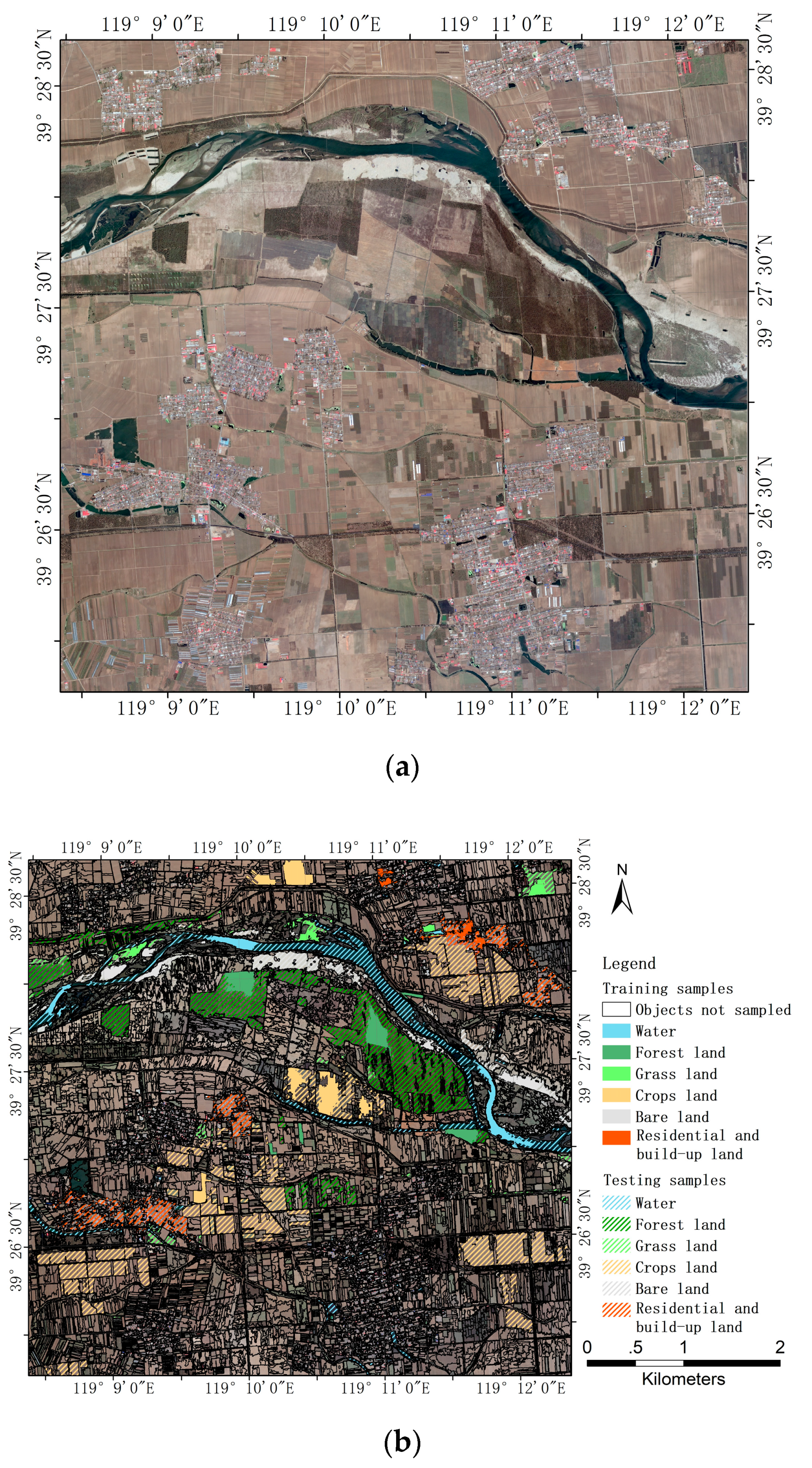
2.1. Data and Study Area
2.2. Segmentation and Sampling
2.3. Group Features
2.4. Feature Ranking
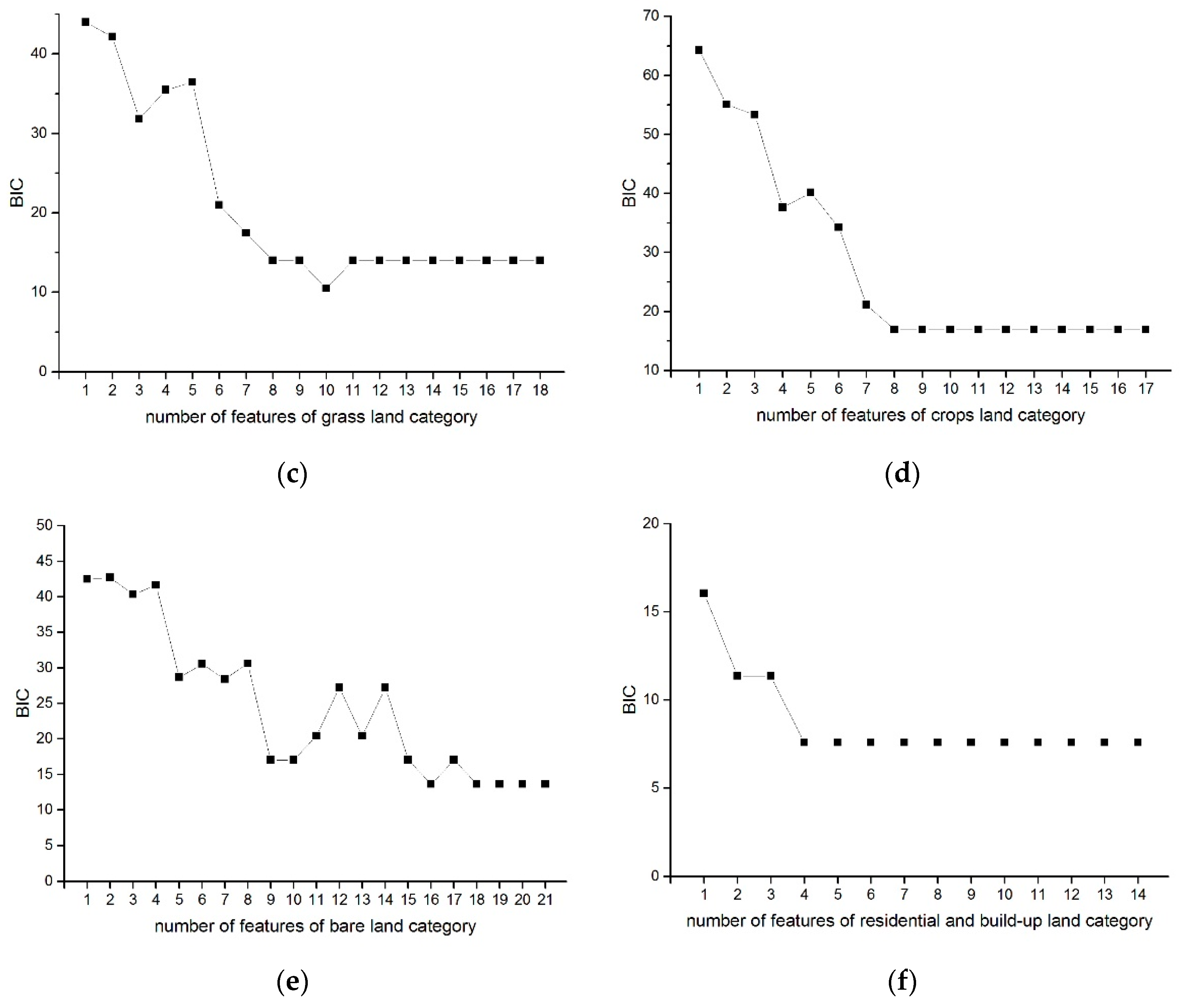
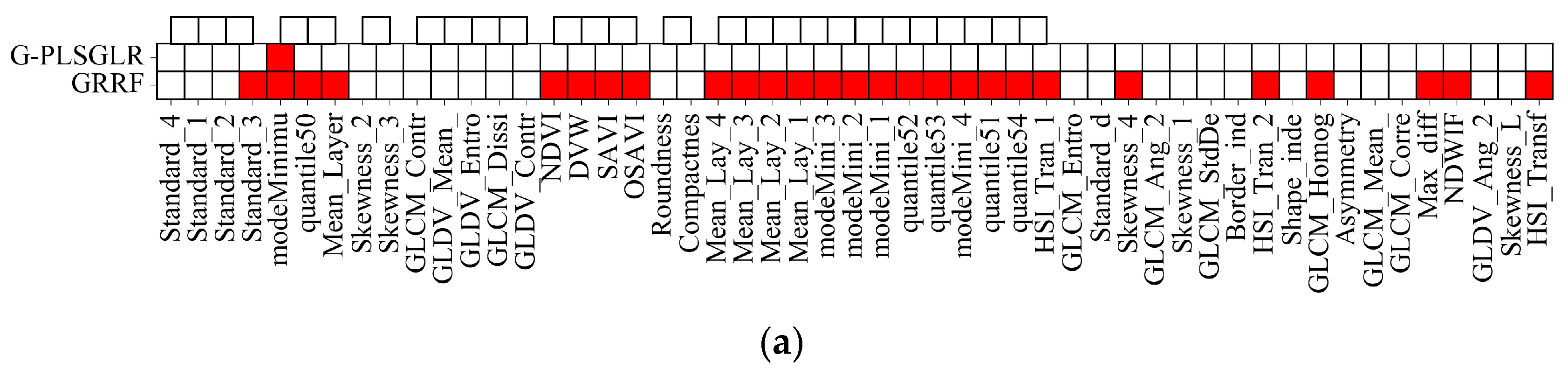
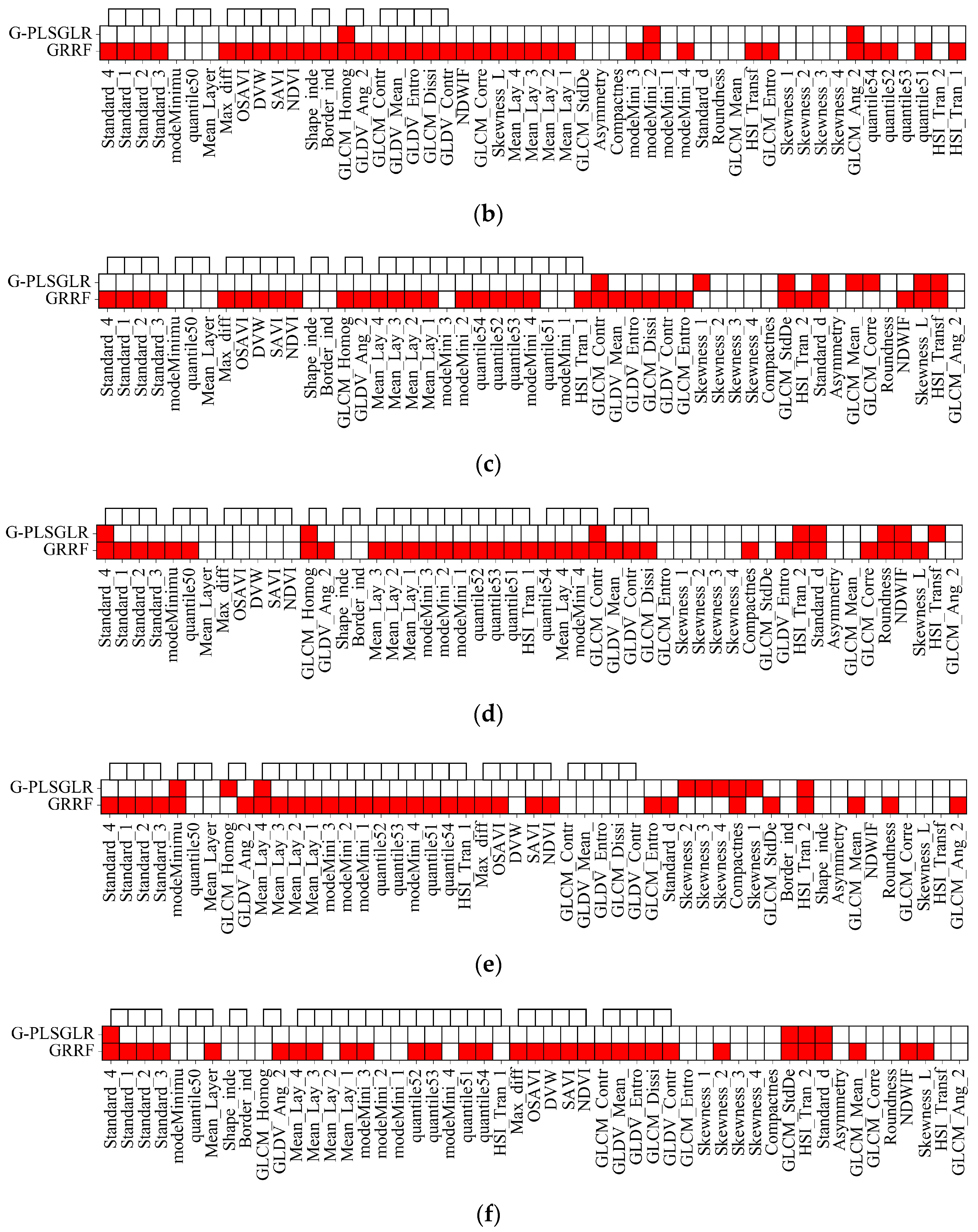
2.5. Feature Selection
3. Results
4. Discussion
4.1. Validation
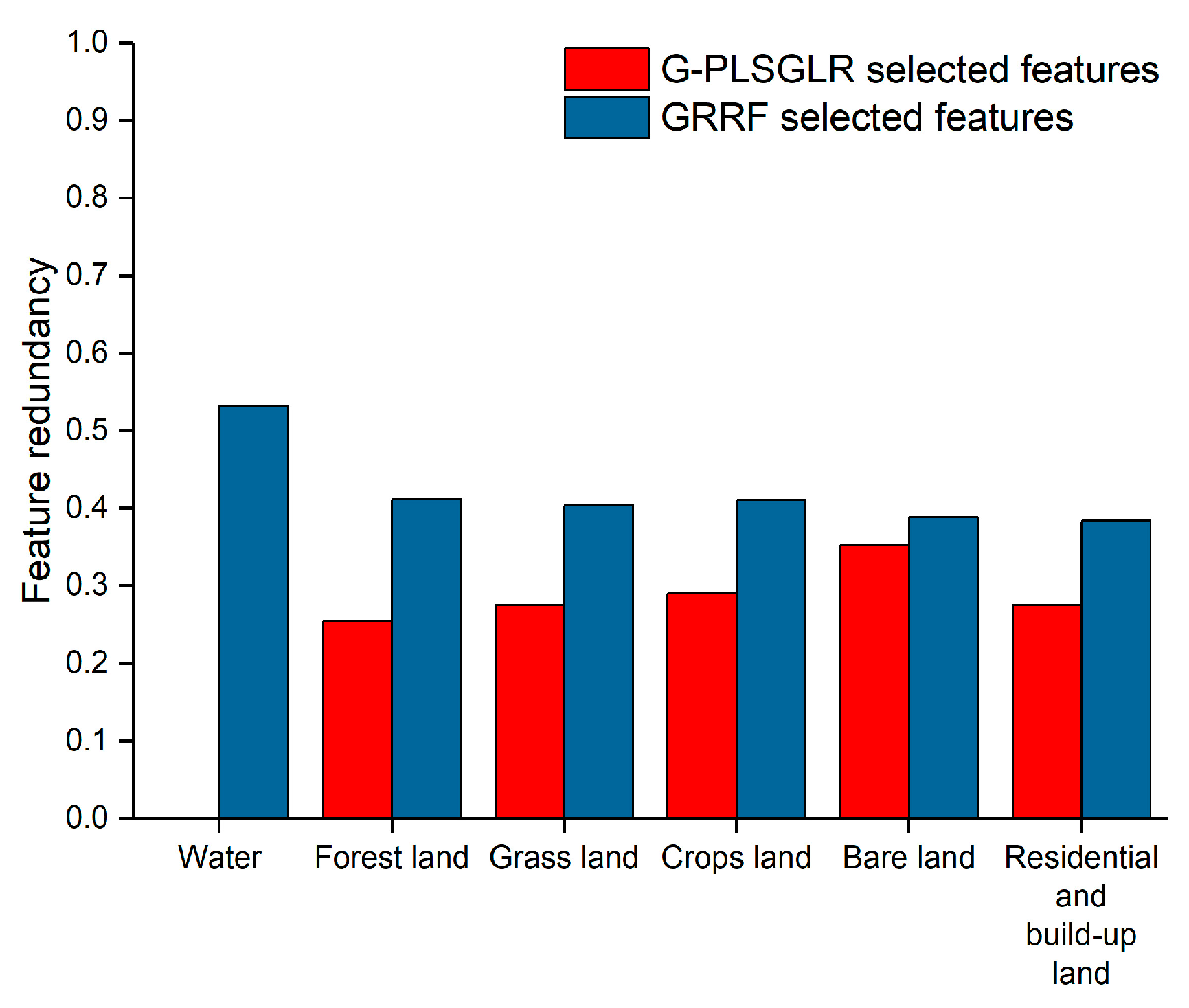
4.1.1. Evaluation of Feature Redundancy
4.1.2. Accuracy Assessment on Selected Features
4.2. Comparison with Other Low Sample Size Studies
4.3. Potential Extensions for Producing Multi-Class Land Use and Land Cover Maps
5. Conclusions
Acknowledgments
Author Contributions
Conflicts of Interest
References
- Ochoa, P.; Fries, A.; Mejía, D.; Burneo, J.; Ruíz-Sinoga, J.; Cerdà, A. Effects of climate, land cover and topography on soil erosion risk in a semiarid basin of the Andes. Catena 2016, 140, 31–42. [Google Scholar] [CrossRef]
- Godinho, S.; Guiomar, N.; Machado, R.; Santos, P.; Sá-Sousa, P.; Fernandes, J.P.; Neves, N.; Pinto-Correia, T. Assessment of environment, land management, and spatial variables on recent changes in montado land cover in southern Portugal. Agrofor. Syst. 2016, 90, 177–192. [Google Scholar] [CrossRef]
- Zhou, G.; Wei, X.; Chen, X.; Zhou, P.; Liu, X.; Xiao, Y.; Sun, G.; Scott, D.F.; Zhou, S.; Han, L. Global pattern for the effect of climate and land cover on water yield. Nat. Commun. 2015, 6, 1–8. [Google Scholar] [CrossRef] [PubMed]
- Tuanmu, M.N.; Jetz, W. A global 1-km consensus land-cover product for biodiversity and ecosystem modelling. Glob. Ecol. Biogeogr. 2014, 23, 1031–1045. [Google Scholar] [CrossRef]
- Mahmood, R.; Pielke, R.A.; Hubbard, K.G.; Niyogi, D.; Dirmeyer, P.A.; McAlpine, C.; Carleton, A.M.; Hale, R.; Gameda, S.; Beltrán-Przekurat, A.; et al. Land cover changes and their biogeophysical effects on climate. Int. J. Climatol. 2014, 34, 929–953. [Google Scholar] [CrossRef]
- Verburg, P.H.; Mertz, O.; Erb, K.-H.; Haberl, H.; Wu, W. Land system change and food security: Towards multi-scale land system solutions. Curr. Opin. Environ. Sustain. 2013, 5, 494–502. [Google Scholar] [CrossRef] [PubMed]
- Lu, X.; Zhuang, Q. Evaluating climate impacts on carbon balance of the terrestrial ecosystems in the Midwest of the United States with a process-based ecosystem model. Mitig. Adapt. Strateg. Glob. Chang. 2010, 15, 467–487. [Google Scholar] [CrossRef]
- Ban, Y.; Gong, P.; Giri, C. Global land cover mapping using earth observation satellite data: Recent progresses and challenges. ISPRS J. Photogramm. Remote Sens. 2015, 103, 1–6. [Google Scholar] [CrossRef]
- Jiang, D.; Huang, Y.; Zhuang, D.; Zhu, Y.; Xu, X.; Ren, H. A Simple Semi-Automatic Approach for Land Cover Classification from Multispectral Remote Sensing Imagery. Available online: http://journals.plos.org/plosone/article?id=10.1371/journal.pone.0045889 (accessed on 8 September 2017).
- Gong, P. Remote sensing of environmental change over China: A review. Chin. Sci. Bull. 2012, 57, 2793–2801. [Google Scholar] [CrossRef]
- Blaschke, T.; Hay, G.J.; Kelly, M.; Lang, S.; Hofmann, P.; Addink, E.; Feitosa, R.Q.; van der Meer, F.; van der Werff, H.; van Coillie, F.; et al. Geographic object-based image analysis–towards a new paradigm. ISPRS J. Photogramm. Remote Sens. 2014, 87, 180–191. [Google Scholar] [CrossRef] [PubMed]
- Hay, G.; Niemann, K.; McLean, G. An object-specific image-texture analysis of H-resolution forest imagery. Remote Sens. Environ. 1996, 55, 108–122. [Google Scholar] [CrossRef]
- Stumpf, A.; Kerle, N. Object-oriented mapping of landslides using random forests. Remote Sens. Environ. 2011, 115, 2564–2577. [Google Scholar] [CrossRef]
- Dronova, I.; Gong, P.; Wang, L. Object-based analysis and change detection of major wetland cover types and their classification uncertainty during the low water period at Poyang Lake, China. Remote Sens. Environ. 2011, 115, 3220–3236. [Google Scholar] [CrossRef]
- Blaschke, T. Object based image analysis for remote sensing. ISPRS J. Photogramm. Remote Sens. 2010, 65, 2–16. [Google Scholar] [CrossRef]
- Formaggio, A.R.; Vieira, M.A.; Rennó, C.D. Object Based Image Analysis (OBIA) and Data Mining (DM) in Landsat time series for mapping soybean in intensive agricultural regions. In Proceedings of the Geoscience and Remote Sensing Symposium (IGARSS), Munich, Germany, 22–27 July 2012. [Google Scholar]
- Huang, X.; Lu, Q.; Zhang, L. A multi-index learning approach for classification of high-resolution remotely sensed images over urban areas. ISPRS J. Photogramm. Remote Sens. 2014, 90, 36–48. [Google Scholar] [CrossRef]
- Powell, W.B. Approximate Dynamic Programming: Solving the Curses of Dimensionality; John Wiley & Sons: Hoboken, NJ, USA, 2007; Volume 703. [Google Scholar]
- Jensen, J.R. Remote Sensing of the Environment: An Earth Resource Perspective 2/E. 2009. Available online: https://s3.amazonaws.com/academia.edu.documents/31163537/08_rs_vegetation.pdf?AWSAccessKeyId=AKIAIWOWYYGZ2Y53UL3A&Expires=1505103677&Signature=L37TIijB8tcuCXSiqYYFP%2BJ8fB0%3D&response-content-disposition=inline%3B%20filename%3DRemote_Sensing_of_the_Environment_An_Ear.pdf (accessecd on 11 September 2017).
- Tang, J.; Alelyani, S.; Liu, H. Feature Selection for Classification: A Review. 2014. Available online: http://eprints.kku.edu.sa/170/1/feature_selection_for_classification.pdf (accessed on 8 September 2017).
- Wu, B.; Xiong, Z.-G.; Chen, Y.-Z. Classification of quickbird image with maximal mutual information feature selection and support vector machine. Procedia Earth Planet. Sci. 2009, 1, 1165–1172. [Google Scholar] [CrossRef]
- Ma, L.; Cheng, L.; Li, M.; Liu, Y.; Ma, X. Training set size, scale, and features in geographic object-based image analysis of very high resolution unmanned aerial vehicle imagery. ISPRS J. Photogramm. Remote Sens. 2015, 102, 14–27. [Google Scholar] [CrossRef]
- Hall, M.A.; Smith, L.A. Feature selection for machine learning: Comparing a correlation-based filter approach to the wrapper. In Proceedings of the Twelfth International Florida Artificial Intelligence Research Society Conference, Orlando, FL, USA, 1–5 May 1999. [Google Scholar]
- Van Coillie, F.M.; Verbeke, L.P.; De Wulf, R.R. Feature selection by genetic algorithms in object-based classification of IKONOS imagery for forest mapping in Flanders, Belgium. Remote Sens. Environ. 2007, 110, 476–487. [Google Scholar] [CrossRef]
- Chen, Q.; Chen, Y.; Jiang, W. Genetic particle swarm optimization–based feature selection for very-high-resolution remotely sensed imagery object change detection. Sensors 2016, 16, 1204. [Google Scholar] [CrossRef] [PubMed]
- Takayama, T.; Iwasaki, A. Optimal wavelength selection on hyperspectral data with fused lasso for biomass estimation of tropical rain forest. ISPRS Ann. Photogramm. Remote Sens. Spat. Inf. Sci. 2016, Ш-8, 101–108. [Google Scholar] [CrossRef]
- Mureriwa, N.; Adam, E.; Sahu, A.; Tesfamichael, S. Examining the spectral separability of Prosopis glandulosa from co-existent species using field spectral measurement and guided regularized random forest. Remote Sens. 2016, 8, 144. [Google Scholar] [CrossRef]
- Fauvel, M.; Tarabalka, Y.; Benediktsson, J.A.; Chanussot, J.; Tilton, J.C. Advances in spectral-spatial classification of hyperspectral images. Proc. IEEE 2013, 101, 652–675. [Google Scholar] [CrossRef]
- Plaza, A.; Benediktsson, J.A.; Boardman, J.W.; Brazile, J.; Bruzzone, L.; Camps-Valls, G.; Chanussot, J.; Fauvel, M.; Gamba, P.; Gualtieri, A. Recent advances in techniques for hyperspectral image processing. Remote Sens. Environ. 2009, 113, S110–S122. [Google Scholar] [CrossRef]
- Ghamisi, P.; Couceiro, M.S.; Benediktsson, J.A. A novel feature selection approach based on FODPSO and SVM. IEEE Trans. Geosci. Remote Sens. 2015, 53, 2935–2947. [Google Scholar] [CrossRef]
- Li, C.; Wang, J.; Wang, L.; Hu, L.; Gong, P. Comparison of classification algorithms and training sample sizes in urban land classification with Landsat thematic mapper imagery. Remote Sens. 2014, 6, 964–983. [Google Scholar] [CrossRef]
- Kavzoglu, T.; Colkesen, I. The effects of training set size for performance of support vector machines and decision trees. In Proceedings of the 10th International Symposium on Spatial Accuracy Assessment in Natural Resources and Environmental Sciences, Florianopolis-SC, Brazil, 10–13 July 2012. [Google Scholar]
- Otto, M. Chemometrics: Statistics and Computer Application in Analytical Chemistry; John Wiley & Sons: Hoboken, NJ, USA, 1998. [Google Scholar]
- Boulesteix, A.L.; Lambert-Lacroix, S.; Peyre, J.; Strimmer, K. Plsgenomics: PLS Analyses for Genomics. R Package Version. 2011. Available online: https://rdrr.io/cran/plsgenomics (accessed on 11 September 2017).
- Brown, D.J.; Shepherd, K.D.; Walsh, M.G.; Mays, M.D.; Reinsch, T.G. Global soil characterization with vnir diffuse reflectance spectroscopy. Geoderma 2006, 132, 273–290. [Google Scholar] [CrossRef]
- Felde, G.; Anderson, G.; Cooley, T.; Matthew, M.; Berk, A.; Lee, J. Analysis of Hyperion data with the FLAASH atmospheric correction algorithm. In Proceedings of the Geoscience and Remote Sensing Symposium, Toulouse, France, 21–25 July 2003. [Google Scholar]
- Drăguţ, L.; Csillik, O.; Eisank, C.; Tiede, D. Automated parameterisation for multi-scale image segmentation on multiple layers. ISPRS J. Photogramm. Remote Sens. 2014, 88, 119–127. [Google Scholar] [CrossRef] [PubMed]
- Yen, S.-J.; Lee, Y.-S. Cluster-based under-sampling approaches for imbalanced data distributions. Expert Syst. Appl. 2009, 36, 5718–5727. [Google Scholar] [CrossRef]
- He, H.; Garcia, E.A. Learning from imbalanced data. IEEE Trans. Knowl. Data Eng. 2009, 21, 1263–1284. [Google Scholar]
- Friedman, J.; Hastie, T.; Tibshirani, R. A Note on the Group Lasso and a Sparse Group Lasso. 2010. Available online: https://arxiv.org/pdf/1001.0736.pdf (accessed on 8 September 2017).
- Haindl, M.; Somol, P.; Ververidis, D.; Kotropoulos, C. Feature selection based on mutual correlation. In Proceedings of the 11th Iberoamerican Congress in Pattern Recognition, Cancun, Mexico, 14–17 November 2006. [Google Scholar]
- Bertrand, F.; Maumy-Bertrand, M.; Meyer, N. Plsrglm, PLS generalized linear models for the R language. In Proceedings of the 12th International Conference on Chemometrics in Analytical Chemistry, Anvers, Belgium, 19 October 2010. [Google Scholar]
- Bertrand, F.; Magnanensi, J.; Meyer, N.; Maumy-Bertrand, M. Plsrglm: Algorithmic Insights and Applications. 2014. Available online: ftp://alvarestech.com/pub/plan/R/web/packages/plsRglm/vignettes/plsRglm.pdf (accessed on 8 September 2017).
- Boulesteix, A.-L.; Strimmer, K. Partial least squares: A versatile tool for the analysis of high-dimensional genomic data. Brief. Bioinform. 2007, 8, 32–44. [Google Scholar] [CrossRef] [PubMed] [Green Version]
- Bastien, P.; Vinzi, V.E.; Tenenhaus, M. PLS generalised linear regression. Comput. Stat. Data Anal. 2005, 48, 17–46. [Google Scholar] [CrossRef]
- Chun, H.; Keleş, S. Sparse Partial Least Squares Regression for Simultaneous Dimension Reduction and Variable Selection. 2010. Available online: http://onlinelibrary.wiley.com/doi/10.1111/j.1467-9868.2009.00723.x/full (accessed on 8 September 2017).
- Akaike, H. A new look at the statistical model identification. IEEE Trans. Autom. Control. 1974, 19, 716–723. [Google Scholar] [CrossRef]
- Deng, H. Guided Random Forest in the RRF Package. 2013. Available online: https://arxiv.org/pdf/1306.0237.pdf (accessed on 8 September 2017).
- Khalid, S.; Khalil, T.; Nasreen, S. A survey of feature selection and feature extraction techniques in machine learning. In Proceedings of the Science and Information Conference (SAI), London, UK, 27–29 August 2014. [Google Scholar]
- Congalton, R.G. A review of assessing the accuracy of classifications of remotely sensed data. Remote Sens. Environ. 1991, 37, 35–46. [Google Scholar] [CrossRef]
- Graves, S.J.; Asner, G.P.; Martin, R.E.; Anderson, C.B.; Colgan, M.S.; Kalantari, L.; Bohlman, S.A. Tree species abundance predictions in a tropical agricultural landscape with a supervised classification model and imbalanced data. Remote Sens. 2016, 8, 161. [Google Scholar] [CrossRef]
- Millard, K.; Richardson, M. On the importance of training data sample selection in random forest image classification: A case study in peatland ecosystem mapping. Remote Sens. 2015, 7, 8489–8515. [Google Scholar] [CrossRef]
- Millard, K.; Richardson, M. Wetland mapping with LIDAR derivatives, SAR polarimetric decompositions, and LIDAR–SAR fusion using a random forest classifier. Can. J. Remote Sens. 2013, 39, 290–307. [Google Scholar] [CrossRef]
- Fassnacht, F.E.; Neumann, C.; Förster, M.; Buddenbaum, H.; Ghosh, A.; Clasen, A.; Joshi, P.K.; Koch, B. Comparison of feature reduction algorithms for classifying tree species with hyperspectral data on three central european test sites. IEEE J. Sel. Top. Appl. Earth Obs. Remote Sens. 2014, 7, 2547–2561. [Google Scholar] [CrossRef]
- Song, K.; Li, L.; Li, S.; Tedesco, L.; Hall, B.; Li, Z. Hyperspectral retrieval of phycocyanin in potable water sources using genetic algorithm–partial least squares (ga–pls) modeling. Int. J. Appl. Earth Obs. Geoinf. 2012, 18, 368–385. [Google Scholar] [CrossRef]
- Wilson, M.; Ustin, S.L.; Rocke, D. Comparison of Support Vector Machine Classification to Partial Least Squares Dimension Reduction with Logistic Descrimination of Hyperspectral Data. 2003. Available online: https://www.spiedigitallibrary.org/conference-proceedings-of-spie/4886/1/Comparison-of-support-vector-machine-classification-to-partial-least-squares/10.1117/12.463169.short?SSO=1 (accessed on 8 September 2017).
- Sánchez-Maroño, N.; Alonso-Betanzos, A.; García-González, P.; Bolón-Canedo, V. Multiclass classifiers vs multiple binary classifiers using filters for feature selection. In Proceedings of the 2010 international joint conference on Neural networks (IJCNN), Barcelona, Spain, 18–23 July 2010. [Google Scholar]
- Tax, D.M.; Duin, R.P. Using two-class classifiers for multiclass classification. In Proceedings of the 16th International Conference on Pattern Recognition, Quebec City, QC, Canada, 11–15 August 2002. [Google Scholar]
- Begum, S.; Aygun, R.S. Greedy hierarchical binary classifiers for multi-class classification of biological data. Netw. Model. Anal. Health Inform. Bioinform. 2014, 3, 53. [Google Scholar] [CrossRef]
- Tibshirani, R.; Hastie, T. Margin trees for high-dimensional classification. J. Mach. Learn. Res. 2007, 8, 637–652. [Google Scholar]


| Features Category | Object Features | Number of Features |
|---|---|---|
| Spectral | Mean (5), Mode (5), Median (5), Standard deviation (5), Skewness (5), Hue, Saturation, Intensity, Max. Diff. | 29 |
| Geometry | Asymmetry, Border index, Compactness, Shape index, Roundness | 5 |
| Texture | GLCM Homogeneity (all direction), GLCM Contrast (all direction), GLCM Dissimilarity (all direction), GLCM Entropy (all direction), GLCM Ang. 2nd moment (all direction), GLCM Mean (all direction), GLCM Standard Deviation (all direction), GLCM Correlation (all direction), GLDV Mean (all direction), GLDV Contrast (all direction), GLDV Entropy (all direction), GLDV Ang. 2nd moment (all direction) | 12 |
| Customized | NDVI, NDWIF, SAVI, OSAVI, DVW | 5 |
| Total | 51 | |
| Land Cover | Number of Samples | |
|---|---|---|
| Training Objects | Testing Objects | |
| Water | 15 | 113 |
| Forest land | 36 | 258 |
| Grass land | 20 | 67 |
| Crops land | 38 | 212 |
| Bare land | 15 | 85 |
| Residential and build-up land | 27 | 172 |
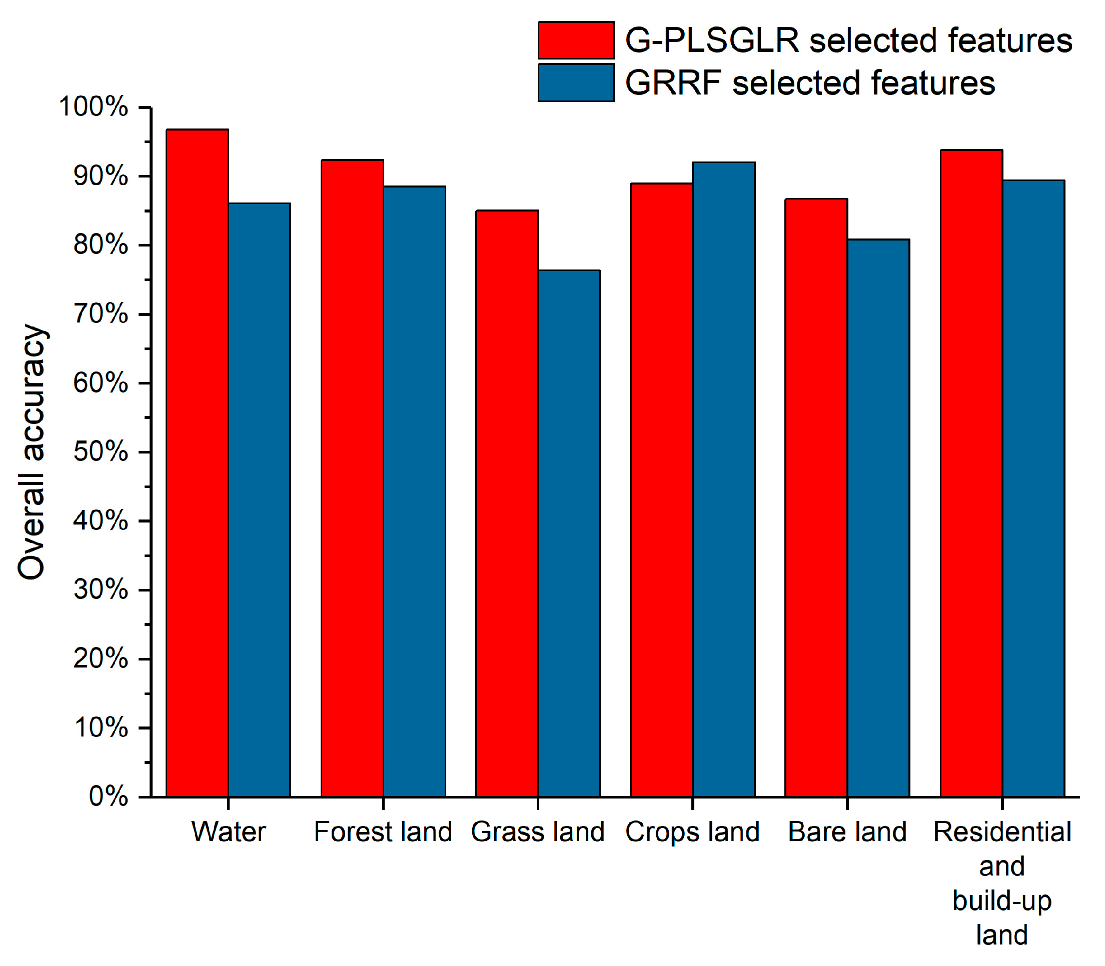
| OA | UA | PA | ||||
|---|---|---|---|---|---|---|
| G-PLSGLR | GRRF | G-PLSGLR | GRRF | G-PLSGLR | GRRF | |
| Water | 96.80% | 86.11% | 80.43% | 47.19% | 98.23% | 96.46% |
| Forest land | 92.39% | 88.53% | 79.44% | 72.38% | 98.84% | 96.51% |
| Grass land | 85.01% | 76.41% | 32.49% | 20.72% | 95.52% | 77.61% |
| Crops land | 88.97% | 92.06% | 68.42% | 75.93% | 98.11% | 96.70% |
| Bare land | 86.77% | 80.82% | 41.03% | 30.90% | 94.12% | 84.71% |
| Residential and build-up land | 93.83% | 89.42% | 76.85% | 64.96% | 96.51% | 95.93% |
© 2017 by the authors. Licensee MDPI, Basel, Switzerland. This article is an open access article distributed under the terms and conditions of the Creative Commons Attribution (CC BY) license (http://creativecommons.org/licenses/by/4.0/).
Share and Cite
Huang, Y.; Zhao, C.; Yang, H.; Song, X.; Chen, J.; Li, Z. Feature Selection Solution with High Dimensionality and Low-Sample Size for Land Cover Classification in Object-Based Image Analysis. Remote Sens. 2017, 9, 939. https://doi.org/10.3390/rs9090939
Huang Y, Zhao C, Yang H, Song X, Chen J, Li Z. Feature Selection Solution with High Dimensionality and Low-Sample Size for Land Cover Classification in Object-Based Image Analysis. Remote Sensing. 2017; 9(9):939. https://doi.org/10.3390/rs9090939
Chicago/Turabian StyleHuang, Yaohuan, Chuanpeng Zhao, Haijun Yang, Xiaoyang Song, Jie Chen, and Zhonghua Li. 2017. "Feature Selection Solution with High Dimensionality and Low-Sample Size for Land Cover Classification in Object-Based Image Analysis" Remote Sensing 9, no. 9: 939. https://doi.org/10.3390/rs9090939