A Feasibility Study of Sea Ice Motion and Deformation Measurements Using Multi-Sensor High-Resolution Optical Satellite Images


Unit of Arctic Sea-Ice Prediction, Korea Polar Research Institute, KIOST, Incheon 21990, Korea
*
Author to whom correspondence should be addressed.
Remote Sens. 2017, 9(9), 930; https://doi.org/10.3390/rs9090930
Submission received: 31 July 2017
/
Revised: 31 August 2017
/
Accepted: 6 September 2017
/
Published: 8 September 2017
(This article belongs to the Section Ocean Remote Sensing)
Abstract
:Sea ice motion and deformation have generally been measured using low-resolution passive microwave or mid-resolution radar remote sensing datasets of daily (or few days) intervals to monitor long-term trends over a wide polar area. This feasibility study presents an application of high-resolution optical images from operational satellites, which have become more available in polar regions, for sea ice motion and deformation measurements. The sea ice motion, i.e., Lagrangian vector, is measured by using a maximum cross-correlation (MCC) technique and multi-temporal high-resolution images acquired on 14–15 August 2014 from multiple spaceborne sensors on board Korea Multi-Purpose Satellites (KOMPSATs) with short acquisition time intervals. The sea ice motion extracted from the six image pairs of the spatial resolutions were resampled to 4 m and 15 m yields with vector length measurements of 57.7 m root mean square error (RMSE) and −11.4 m bias and 60.7 m RMSE and −13.5 m bias, respectively, compared with buoy location records. The errors from both resolutions indicate more accurate measurements than from conventional sea ice motion datasets from passive microwave and radar data in ice and water mixed surface conditions. In the results of sea ice deformation caused by interaction of individual ice floes, while free drift patterns of ice floes were delineated from the 4 m spatial resolution images, the deformation was less revealing in the 15 m spatial resolution image pairs due to emphasized discretization uncertainty from coarser pixel sizes. The results demonstrate that using multi-temporal high-resolution optical satellite images enabled precise image block matching in the melting season, thus this approach could be used for expanding sea ice motion and deformation dataset, with an advantage of frequent image acquisition capability in multiple areas by means of many operational satellites.
1. Introduction
Sea ice motion and deformation measured from satellite remote sensing have played a significant role in understanding the dynamic polar climate system and to predict its ongoing and further long-term changes. Sea ice motion has been measured using low-resolution (e.g., a spatial resolution of 1 km or larger pixel size) satellite remote sensing datasets such as passive microwave data (e.g., Scanning Multichannel Microwave Radiometer (SMMR) [1], Special Sensor Microwave/Imager (SSM/I) [1,2,3,4,5] and Advanced Microwave Scanning Radiometer for the Earth Observing System (EOS) (AMSR-E) [4,6,7]) and optical image data (e.g., Advanced Very High Resolution Radiometer (AVHRR) [8,9]) from a regional-scale (e.g., polynya or basin) to the entire Arctic or Southern Ocean.
Relatively higher spatial resolution satellite radar remote sensing with a spatial resolution from several tens of meters to around a hundred meters) has rarely been applied to the measurement of sea ice motion (e.g., RADARSAT Geophysical processor system (RGPS) [10], GlobICE using Advanced Synthetic Aperture Radar (ASAR) on Envisat, with a spatial resolution of 150 m [11], Envisat ASAR with a spatial resolution of 75 m [12], and RADARSAT-2 ScanSAR of a spatial resolution of 100 m resampled from 50 m [13]). These mid-resolution SAR successfully provided the products from polynya [14] or basin-scale to the entire arctic coverage by systematic data acquisition plan. Radar remote sensing has been recognized as an optimum tool for sea ice motion retrieval because of its all-weather capability and day/night operation; however, operational sensors that can acquire data with proper revisit intervals are limited.
The representative and universal technique to measure sea ice motion by satellite remote sensing is by matching a block of prior images to a corresponding block of posterior images by choosing a maximum cross-correlation (MCC) coefficient, with consideration of the image acquisition time interval [2,4,15]. The image blocks are usually matched in the areas where prominent and contrast features such as the boundary between ice and ocean are dominant. The drawback of the MCC approach is quantization noise, a degree of discreteness of the motion vector field, related to image pixel size [4,10].
Sea ice motion can be directly linked to sea ice deformation because the deformation is calculated from spatial gradients of motion [16]. Therefore, satellite radar remote sensing with sub-daily to few days data acquisition intervals has been widely applied to measure the deformation [16,17]. Few sub-daily deformation measurements were reported in Reference [18]; however, further studies regarding longer periods with short and continuous observation for more detailed understanding of the deformation as a mixture of inertial motion, tidal effect, and wind forcing are necessary [19]. As low-contrast backscatter conditions on the sea ice surface during the melting season or sea ice edge area increases uncertainties in block matching between sequential images, the deformation data were commonly limited to the spring, fall and winter seasons [7], or restricted on inner pack ice areas except ice margins [16].
The possible utility of high-resolution optical satellite images for sea ice motion retrieval was suggested via visual inspection [20]. High-resolution optical airborne observation was applied to measure high temporal and spatial resolution sea ice motion in near real-time [21], but limited to coastal areas because of the coverage restriction of aerial survey. Small-scale kinematics (i.e., deformation) including opening and closing along the fractures in ice cover that can be connected to cracks exposing ocean and altering surface heat balance, and forcing ice into pressure ridges increasing drags between ice-ocean were detected from literal image derived product (LIDP), 1-m resolution panchromatic optical images [22]. This application of high-resolution optical satellite images to sea ice deformation measurement provided smaller scale deformation than the mid-resolution radar remote sensing with spatial resolutions from several tens of meters to around a hundred meters [10,11,12,13,14].
Measuring sea ice motion from the low-resolution satellite datasets have been validated using buoy location records [23]. However, it is difficult to obtain the reference data for the validation because location records from buoy or ice drift station are sparse. To overcome deficiency of reference dataset, alternative validation approaches have been devised, e.g., assessing suitability of image blocks for matching [24].
Nowadays, high-resolution optical imaging satellites have become more available. Moreover, earth observing near-polar orbit satellites have an advantage on more frequent visiting in high-latitude regions as trajectories converge around polar regions [25]. Although optical satellite remote sensing is limited to cloud free conditions, combinations of sequential high-resolution optical images acquired from operational multiple sensors in high latitude regions can contribute to measuring long-term trends in ice motion, and can also be a reliable tool for monitoring sea ice in shipping lanes or in the vicinity of oil and gas platforms.
This study aimed to evaluate the feasibility of multi-sensor high-resolution optical satellite remote sensing for precise sea ice motion measuring using an MCC approach. To validate the measured sea ice motion, a comparison of the high- and resampled mid-resolution satellite image-derived sea ice motion with buoy trajectory was demonstrated, and causes of measurement errors (considering the effects from degraded spatial resolution) were investigated. Additionally, from the sea ice motion data, the sea ice deformation was estimated, and the applicability of the multi-sensor high-resolution optical satellite images for measuring kinematic characteristics of sea ice discussed.
2. Materials
2.1. Description of Study Area
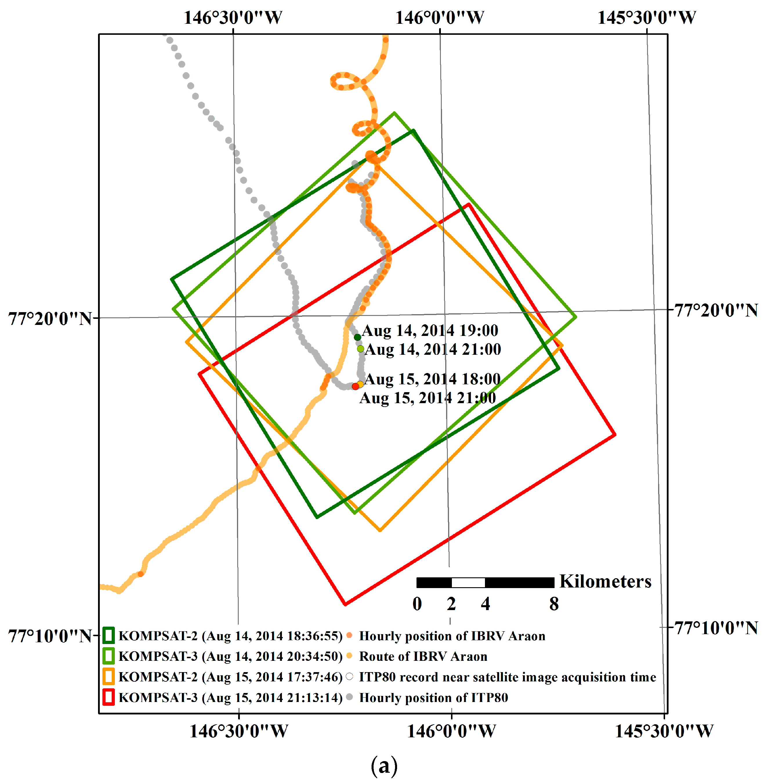
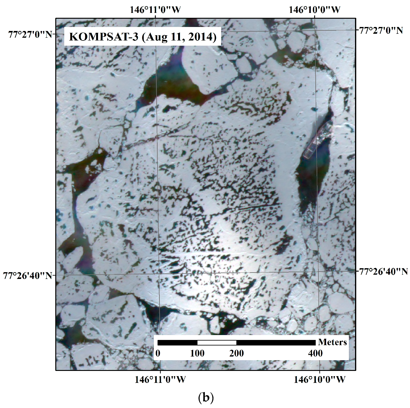
The study area was located around 77°20′N/146°10′W in the Beaufort Sea, where a field investigation on sea ice was conducted in August 2014 (Figure 1a). During the sea ice field investigation, an Ice-Tethered Profiler 80 (ITP80) buoy was deployed on an ice floe where the Korean Icebreaker Research Vessel (IBRV) Araon was anchored (Figure 1b). After deployment of the ITP80, high-resolution optical satellite images were sequentially acquired from the Korea Multi-Purpose Satelllite-2 (KOMPSAT-2) and Korea Multi-Purpose Satelllite-3 (KOMPSAT-3), so that the ITP80 deployed ice floe was captured within the images in the study areas.
2.2. Acquisition of Dataset
2.2.1. High-Resolution Satellite Image
The KOMPSAT-2 and KOMPSAT-3 satellites, with payloads of optical imaging sensors, were employed to acquire high-resolution images. The sensors equipped on the satellites enabled the acquisition of one panchromatic (PAN) and four multispectral (MS) bands (Table 1). The KOMPSAT-2 Multispectral Camera’s (MSC’s) spatial resolutions were 1.0 m for the PAN and 4.0 m for the MS bands, and the KOMPSAT-3 Advanced Earth Imaging Sensor System’s (AEISS’s) spatial resolutions were 0.7 m for the PAN and 2.8 m for the MS bands, respectively.
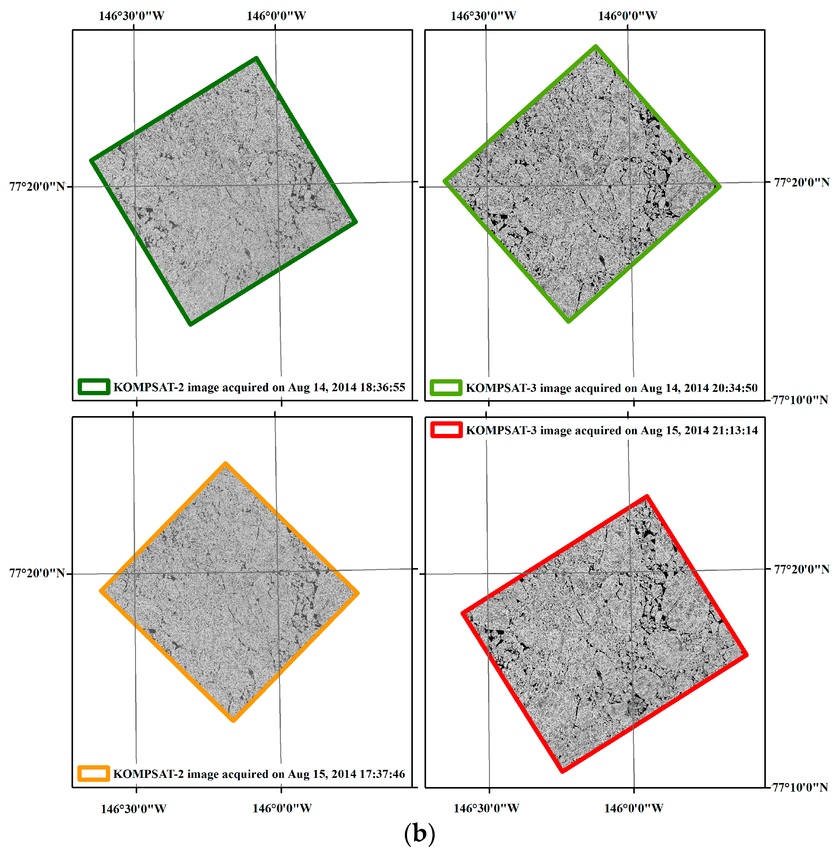
Four images were successively acquired during 14–15 August 2014 (Table 2). From the time gap between the local mean time on ascending nodes of the satellites, the image acquisition times within a day were not identical, so the images acquired in a day from different satellites enabled them to be compared with each other.
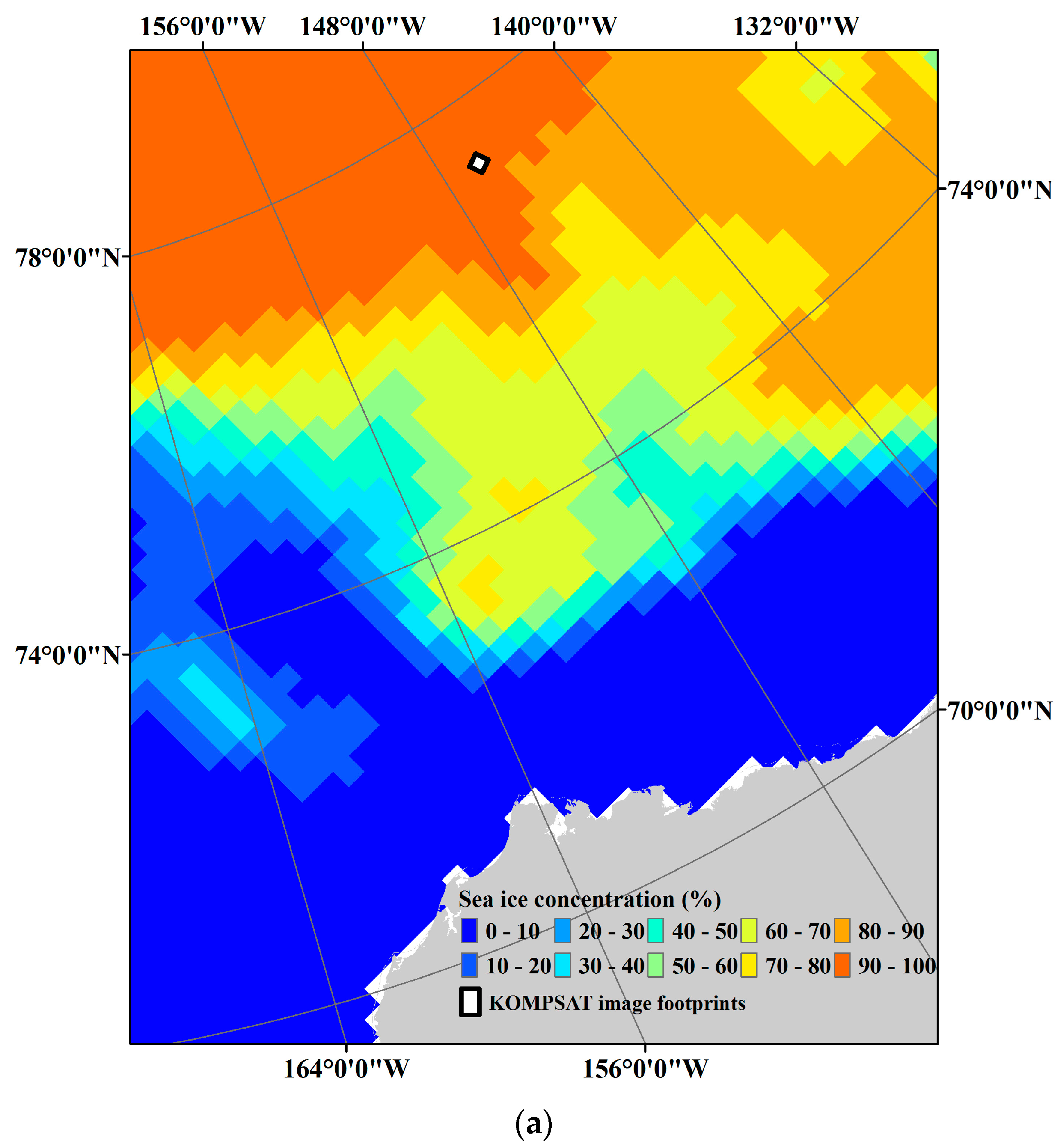
Sea ice conditions on 14 August 2014 around the study area were estimated in the range of 90–100% sea ice concentration (SIC) from the National Snow and Ice Data Center (NSIDC) (Figure 2). From visual inspection of the satellite images, most of the study area was identified as covered with multi-year ice floes. Between the ice floes, small parts of open oceans were exposed, and many melt ponds occupied the surface of the ice floes.
2.2.2. Ice-Tethered Profiler 80 (ITP80) Buoy Location Record
The Ice-Tethered Profilers (ITPs) were contrived and deployed to repeatedly record various properties, e.g., temperature, salinity and measuring location, of the ice-covered Arctic Ocean, with telemetry and underwater instruments, and the data was transferred by Iridium data telemetry [30]. As part of the Office of Naval Research (ONR) Marginal Ice Zone program, the ITP80 buoy was deployed on a 2.6 m thick ice floe in the Beaufort Sea from the IBRV Araon during the field investigation in August 2014 (Table 3).
The ITP80 data (including its hourly locations) were collected and made available by the Ice-Tethered Profiler Program [31,32] based at the Woods Hole Oceanographic Institution [30]. The GPS (Global Positioning System) position in the level 3 archive data of the ITP80 was designated as a reference dataset for validating the sea ice motion from the satellite images.
3. Methods
3.1. Measuring Sea Ice Motion and Deformation
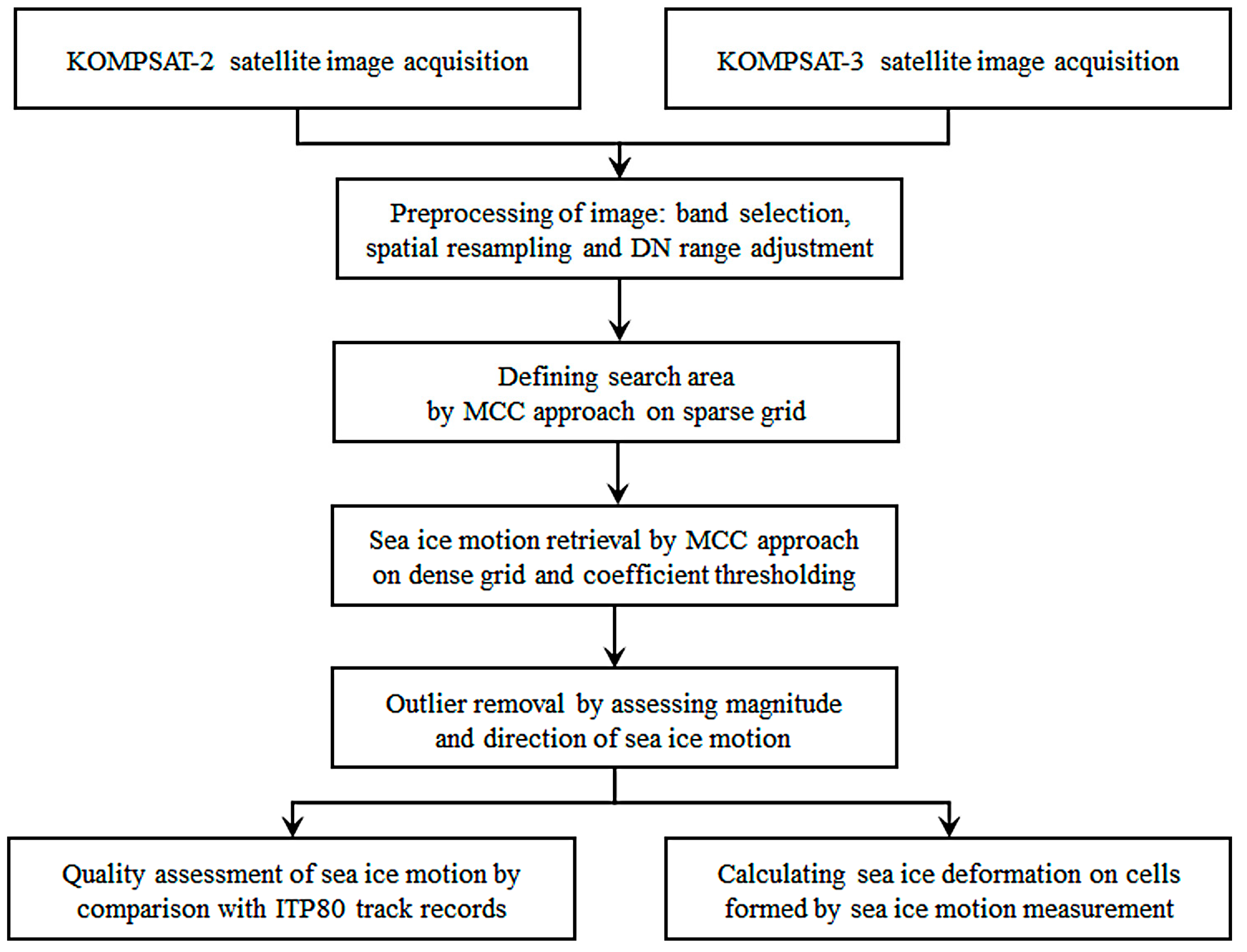
To measure sea ice motion and deformation, a processing chain including preprocessing of the satellite images after the appropriate band selection, measuring the sea ice motion using the MCC technique with hierarchical fashion, conducting a quality assessment on the sea ice motion measurement results, and an investigation on sea ice deformation were implemented (Figure 3).
3.1.1. Preprocessing of Satellite Image
Band saturation in optical remote sensing images (caused by snow and ice covers and showing very high reflectance properties) has been reported in high-latitude regions [33]. To prevent omitting sea ice surface texture details from slight brightness differences among snow, exposed ice from ablation of snow and snow covered or frozen melt pond, pixel value distribution in every MS band was examined, before a common band showing none or a small number of saturated pixels in the images from both satellites was selected for further analyses.
The images obtained from two satellite sensors were basically quantized to 10 bit and 14 bit, respectively (Table 1). To compare pixel value between them (i.e., digital number, DN), ranges for the selected band were equalized by simply multiplying 24 by the 10 bit KOMPSAT-2 image.
Two datasets of high- and mid-resolution were prepared to investigate the feasibility of satellite images of different resolutions for measuring sea ice motion and deformation. In the case of the high-resolution, the KOMPSAT-3 MS bands were resampled to the coarser resolution of 4 m to be identical to the pixel size of the MS bands of the KOMPSAT-2 so a direct comparison between them could be made. For the mid-resolution dataset, the spatial resolutions of the MS bands from both satellites were resampled to 15 m, similar to the images from major mid-resolution optical satellite sensors such as Landsat-7 ETM+ (Enhanced Thematic Mapper Plus), Landsat-8 OLI (Operational Land Imager) and Sentinel-2 MS bands, to investigate the applicability of these mid-resolution satellite images covering wider areas to sea ice motion and deformation measurements. The resampling was conducted by weighted averaging of the input pixel values within the extent of output pixel boundary.
3.1.2. Maximum Cross-Correlation Approach for Measuring Sea Ice Motion
Six image pairs composed of four sequential images were considered for measuring sea ice motion (Table 4). Intervals between the image acquisition times of each image pair varied from about 2 h to about 27 h. Among the image pairs, four pairs consisted of images from different sensors, i.e., the KOMPSAT-2 and KOMPSAT-3, and two pairs consisted of single sensor images.
In the MCC approach, cross-correlation coefficients were calculated between the template window of the prior image and the search area of the posterior image by sliding a search window of identical size of the template window within the search area, before the window pairs revealing maximum cross-correlation coefficient were designated as matching pairs.
To speed up the computation of the cross-correlation coefficients and to avoid false matching occurring in the not overlapped region (without the necessity of prior knowledge about practical moving distance of ice floes), hierarchical fashion was applied. First, the template window size and the sliding distance were set as 75 pixels (300 m) and 300 pixels (1200 m) for the 4 m spatial resolution images, and 75 pixels (1125 m) and 80 pixels (1200 m) for the 15 m spatial resolution images, respectively, to initialize coarse grid points; next, the sea ice motion was delineated from this coarse grid. The search area was formed with the edges apart from the center coordinates of the template window in the posterior image for every template window sliding. The edge lengths of the square-shaped search area varied from three to six times that of the median magnitude of the motion vectors extracted from the coarse grid to form the search area of enough size including common trackable ice floes in sequential images, with consideration of the template window size.
After determining the search area, a finer grid was established as the sliding distance of 30 pixels (120 m) for the 4 m spatial resolution images, and 8 pixels (120 m) for the 15 m spatial resolution images, respectively, and the motion was delineated with the revised sliding distance. This fine grid used to extract the sea ice motion also composed cells for calculating sea ice deformation.
To prevent errors possibly occurring at image borders as a false matching [24], the template windows consisting only of non-zero pixels were considered in the matching procedure, and then the threshold applied to the cross-correlation coefficients for sea ice motion retrieval was set to 0.6. Moreover, remaining outlier motion vectors from the false matching (that could also occur in the regions not exactly overlapped position) between sequential images were filtered and removed where vectors were outside three times the inter-quartile range, if necessary, as the magnitude and direction of the outliers showed large variance compared with the gentle gradient of magnitude and direction in the highly correlated fine grid motion vector field.
Sea ice coverage, a ratio of ice pixels to template window area, in the template window was calculated to understand the effects of complexity of image texture reflecting sea ice conditions on the cross-correlation coefficient. Among various approaches for identifying sea ice concentration from optical images, simple and automated Otsu’s thresholding [34], maximizing inter-class variance, and minimizing intra-class variation of two cluster representing bi-modal histogram [35] were applied.
Additionally, to consider the effect of image complexity in the template window, reflecting randomness of shape features of sea ice such as ice floe size, pressure ridge and melt pond distributions, during the sea ice motion measurement, image entropy was adopted to statistically measure the texture of the image block, as in Equation (1):
where p is the histogram counts for the image in each template window [36].
Entropy = −Σ p × log2(p)
3.1.3. Validating Satellite Image-Derived Sea Ice Motion
A comparison with a Lagrangian buoy track has been generally applied to the validation of satellite image-derived sea ice motion [4,37,38,39,40,41]. For validation of the sea ice motion, first, the locations of the ITP80 buoy (recorded in the closest time of satellite image acquisition times) were linearly interpolated at the prior and posterior image acquisition times. The motion vector of which the center was closest from the center of two time-interpolated locations was retrieved, and the validation performed by comparing the selected satellite image-derived motion vector with the vector connecting the time-interpolated buoy locations [17,42]. The validations for moving distance, direction and velocity were performed for both cases of 4 m and 15 m spatial resolutions. Differences between the GPS based ITP80 motion and satellite image based motion were considered in statistical analyses to estimate bias and root mean square error (RMSE). During the validation, other error sources such as GPS positioning uncertainty and image geolocation errors were also considered.
3.1.4. Measuring Sea Ice Deformation
Sea ice deformation provides information on individual floe size as a separated area by high shear, especially in the application of high-resolution remote sensing, and sea ice kinematics composed of opening from brittle failure and closing forcing ice into pressure ridges [22]. The combination of the opening connected to new ice production from the freezing of the exposed ocean and the closing causing sea ice thickness changes is known to adjust the overall area and volume of sea ice in polar regions.
Strain rate of each cell defined from the sea ice motion grid varies in velocity components, u and v. Invariants of the spatial gradient of the velocity component are calculated using strain rate components with approximations of the line integral around the boundary of each cell [17] using Equations (2) and (3).
To evaluate the applicability of the multi-sensor high-resolution optical satellite images for measuring kinematic characteristics and to examine the effects from different spatial resolution, the divergence and shear were delineated from the image pairs of both spatial resolutions, and spatial patterns and distribution of values were investigated for comparison between the datasets.
4. Results
4.1. Sea Ice Motions from Maximum Cross-Correlation Approach
Among the MS bands of the KOMPSAT images, a common band of least saturated, preserving surface texture details of sea ice, was selected. Few saturated pixels in the red band exist only in the KOMPSAT-2 image acquired on 14 August 2014; therefore, the red band was used for further analyses. Hereafter, images denote the red band image.
The cross-correlation coefficient was measured in whole image pairs of both spatial resolutions using the MCC approach. The histograms of the cross-correlation coefficient showed typical bimodal distribution for both resolutions, discriminating precise sea ice motion from errors that generally originate from matched blocks in a not overlapped image area (Figure 4). Around the predefined threshold value (i.e., cross-correlation coefficient = 0.6), a low amplitude of the histogram indicated that a possible few motion vectors with a higher cross-correlation coefficient than the threshold value existed in the dataset of the spatial resolution of 4 m (Figure 4a), while a more distinct bimodal distribution of the histograms was revealed in the dataset of the spatial resolution of 15 m. After applying outlier removal to remove the few remaining outlier motion vectors in the pairs of the dataset of the spatial resolution of 4 m, well-aligned continuous dense motion vectors without erroneous magnitudes or directions in overlapped areas were retrieved.
The dense distributions of the moving distance and direction (i.e., the magnitude and direction of the motion vectors) from the image pairs of the 4 m spatial resolution revealed spatial patterns reflecting characteristics of sea ice motion (Figure 5).
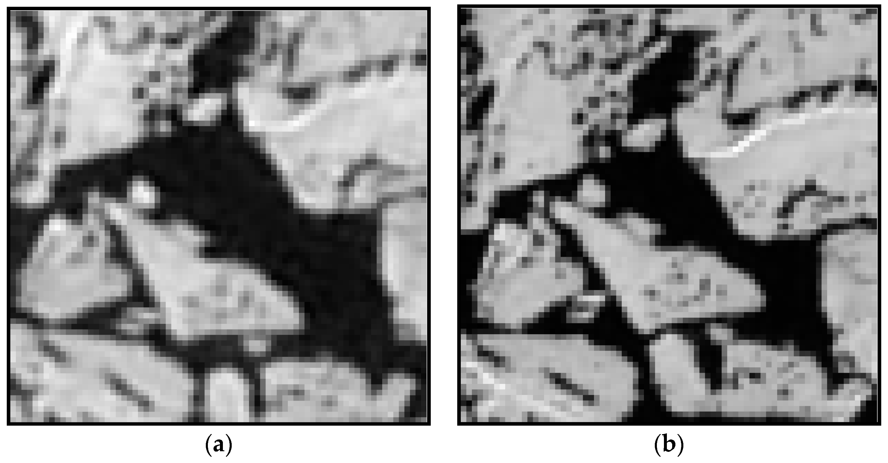
Small vacant spaces in the motion vector fields appeared during the cross-correlation coefficient thresholding caused by free drifted isolated floes, which are seasonal characteristics of sea ice that especially appear in summer that decrease the cross-correlation between sequential images (Figure 6).
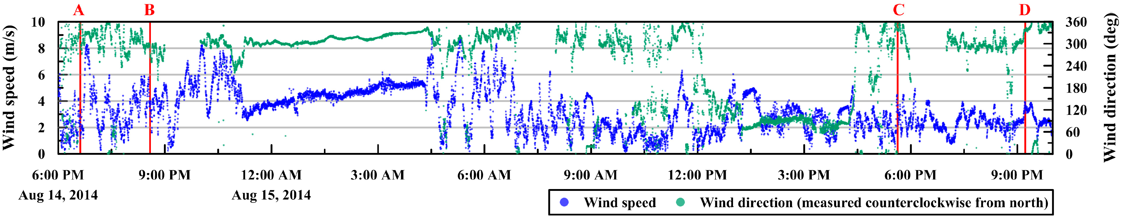
Wind is one of the main factors that controls sea ice motion [43]; therefore, wind direction and speed were measured in the IBRV Araon every second during the image acquisition period (Figure 7). Although the distance between the IBRV Araon and the ITP80 increased from 57.7 km at the acquisition time of image A to 258.7 km at the acquisition time of image D as time passed, the direction of sea ice motion generally corresponds to the wind records of a mainly southward direction.
For the dataset spatially resampled to 15 m, the motion vectors with cross-correlation coefficients higher than the threshold value showed a well-aligned motion field without additional removal of erroneous magnitudes or directions of the motion vectors (Figure 8). Increased sea ice coverage and decreased entropy compared with the same image pair of the spatial resolution of 4 m were observable, and these trends were the same with the other image pairs. Slightly more discrete colors of the motion vectors were revealed in Figure 8a when compared with Figure 5a.
4.2. Quality Assessment of the Sea Ice Motion Measurement
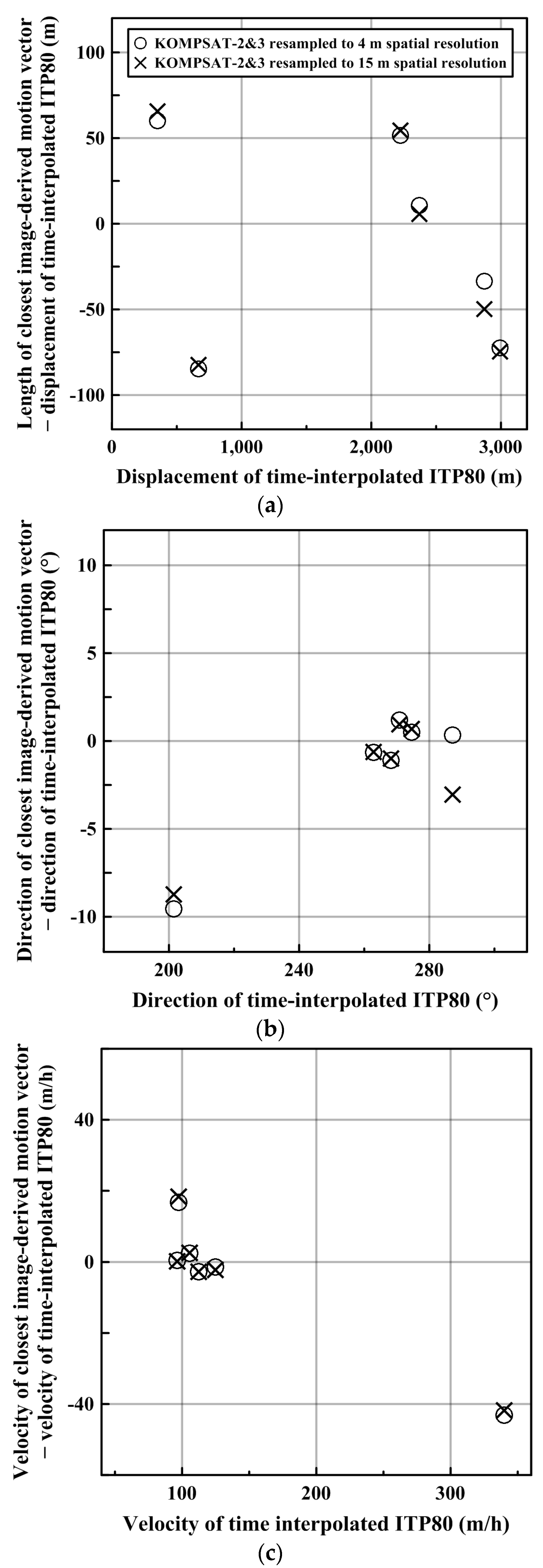
The consistency between the sea ice drifts measured from sequential image pairs and the time-interpolated ITP80 track records indicated the quality of the satellite image-derived sea ice motion measurement. Three parameters including distances, directions and velocities were investigated for both high- and mid-resolution datasets (Figure 9). The image-derived motion vectors of which the center as closest to the center of two time-interpolated locations in each image pair were selected to compare with the motions connecting the time-interpolated buoy locations.
Differences of the displacements, directions and velocities exist between both datasets. The displacements of the spatial resolution of 4 m varied from 409.6–2839.5 m, while the distances of the spatial resolution resampled to 15 m varied from 415.0–2823.4 m (Figure 9a). The velocities of the spatial resolution of 4 m, calculated from the distance divided by the time gap between images within a pair, varied 96.7–296.7 m·h−1, equivalent to 2.7–8.2 cm·s−1, while the velocities of the spatial resolution resampled to 15 m varied 96.5–298.0 m·h−1, equivalent to 2.7–8.3 cm·s−1 (Figure 9b). The directions of the spatial resolution of 4 m varied 192.0–287.5°, while the directions of the spatial resolution resampled to 15 m varied 192.8–284.1° (Figure 9c). Root mean square errors (RMSEs) and biases were calculated from the parameters (Table 5).
4.3. Relationships Between Cross-Correlation Coefficient and Sea Ice Image Properties
In the MCC approach, a high cross-correlation coefficient consolidates more accurate motion measurement without outliers that demand additional removal processes such as filtering or averaging nearby vectors. Links between the cross-correlation coefficient and image properties representing sea ice conditions such as sea ice coverage and entropy of image blocks (i.e., template window images) were assessed to identify the relationships.
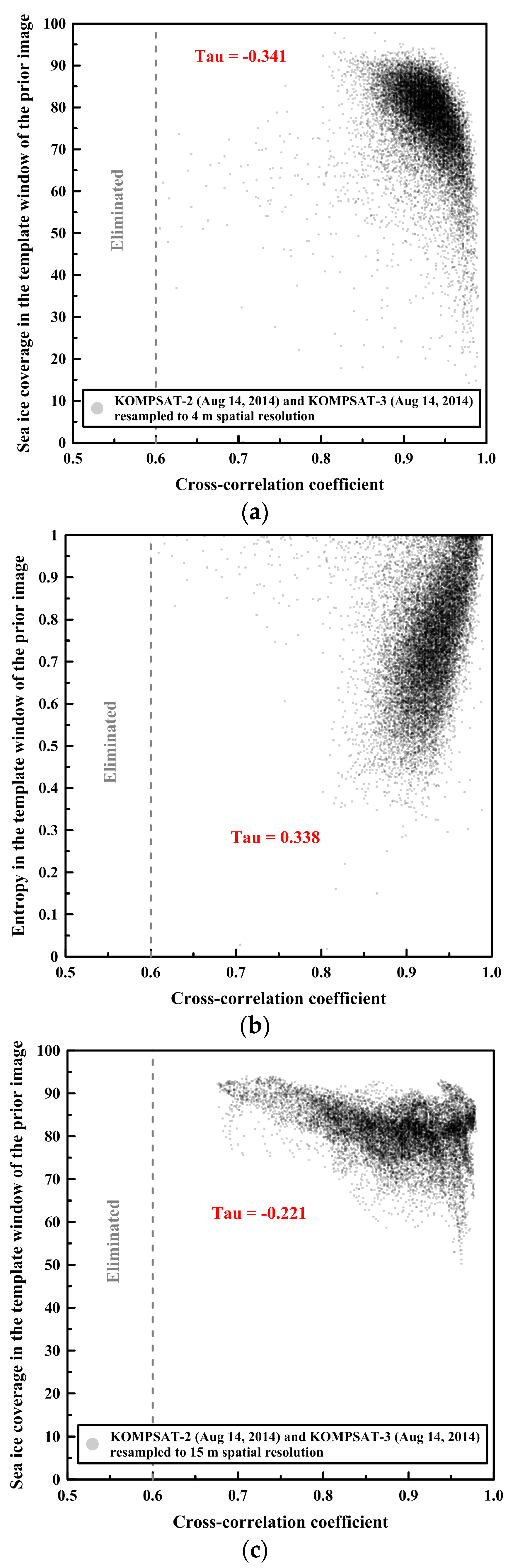
The cross-correlation coefficient and the sea ice coverage of the image blocks from the prior image showed negative correlations as negative Kendall’s tau coefficients, implying ordinal association considering non-parametric variables with ties, in the image pairs of both spatial resolutions [44] (Figure 10a,c).
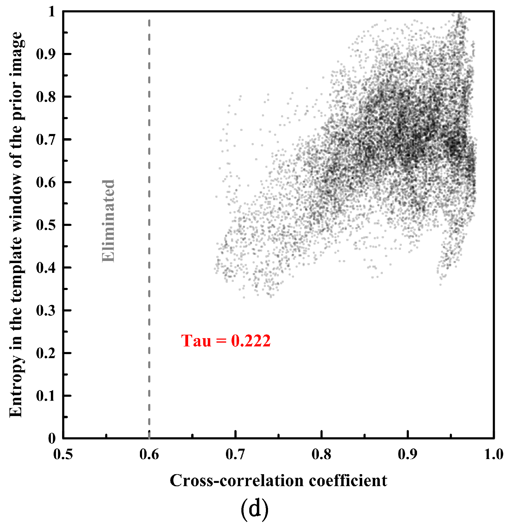
On the other hand, the cross-correlation coefficient and the entropy of the image blocks from the prior image showed positive correlations as positive Kendall’s tau coefficients in the image pairs of both spatial resolutions (Figure 10b,d). The trends of the correlation coefficients (tau) of the other image pairs were similar to Figure 10 (Table 6). The correlation coefficients (tau) between the cross-correlation coefficient and sea ice coverage were negative, and the correlation coefficients (tau) between the cross-correlation coefficient and entropy were positive.
Among the sea ice coverage and the entropy of the matched image block from the pair of the KOMPSAT-2 image acquired on 14 August 2014 (i.e., prior image) and the KOMPSAT-3 image acquired on 14 August 2014 (i.e., posterior image) resampled to the spatial resolution of 4 m (Figure 11), the image block of the prior image showing the maximum sea ice coverage parameter yielded very low entropy, and the image block showing the sea ice coverage parameter of about 50% yielded the maximum entropy. In the case of the sea ice coverage and entropy of the matched block from the same image pair resampled to the spatial resolution of 15 m (Figure 12), an identical trend was observed. Although Figure 11 and Figure 12 are not image blocks in identical locations and areas, it can be inferred that resampling to coarser spatial resolution resulted in a smoothed texture, increased sea ice coverage from the effects of mixing adjacent open water and sea ice pixels, and decreased entropy from more homogenized texture when the image blocks were selected as an identical area.
4.4. Sea Ice Deformation
Openings and closings along the narrow ice fractures bring cracks to expose ocean, which varies surface heat balance, and changes ice into pressure ridges which raise drags between ice and ocean, and ice and atmosphere, and modify ice thickness, respectively [45]. Small-scale kinematics caused by interaction of individual ice floes can be observed from the measurement of the relative motion of ice floes with enough detailed resolution.
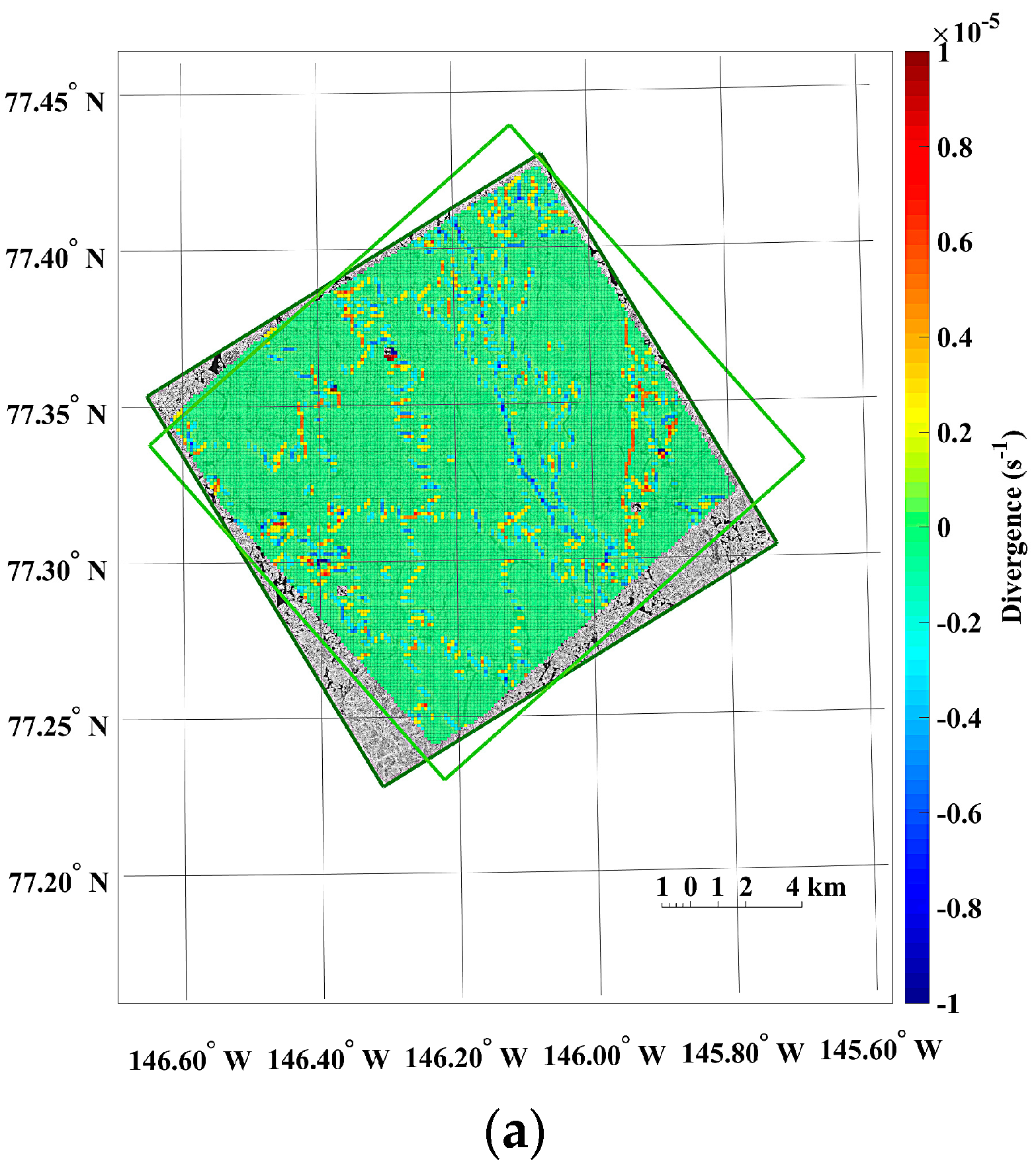
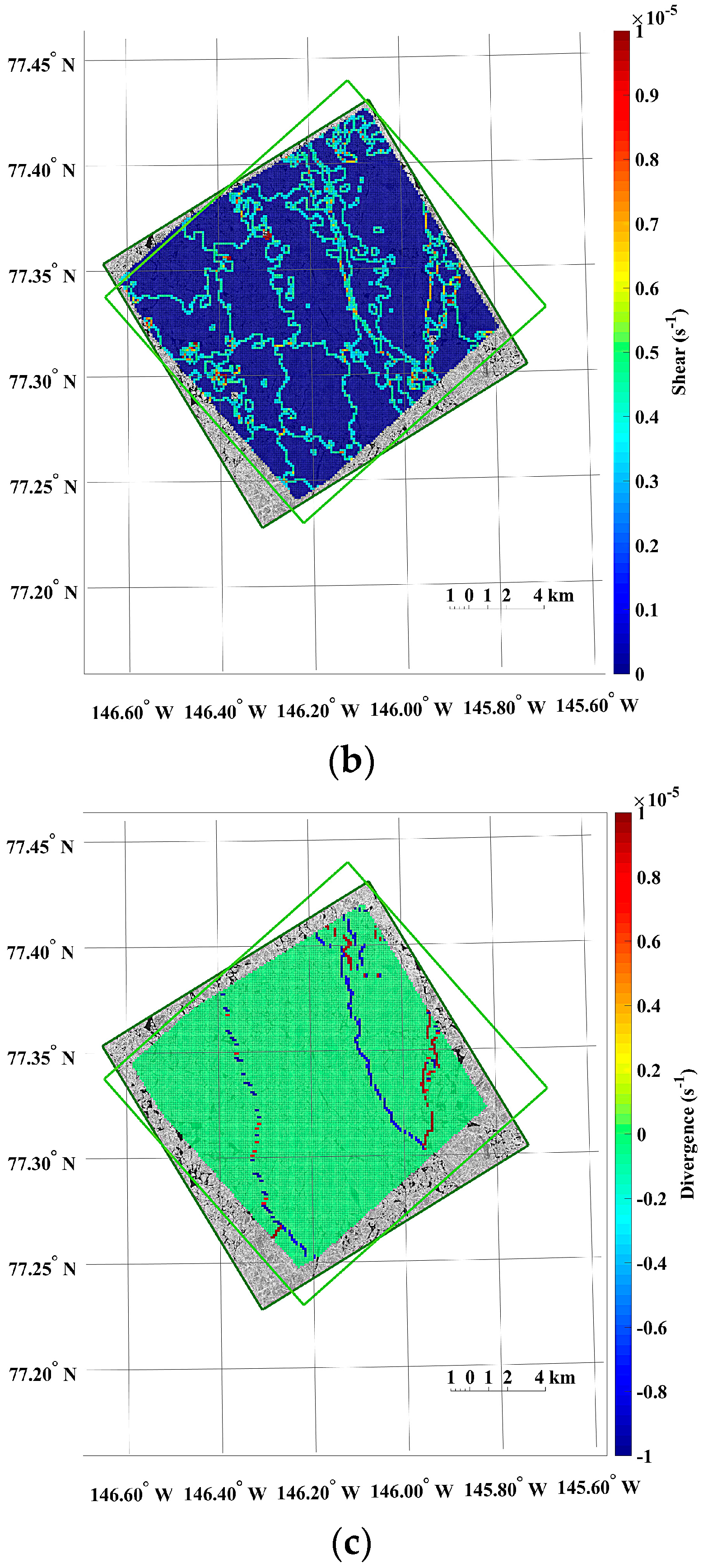
The small-scale kinematics was observable from the sea ice motion field extracted from the KOMPSAT-2 image acquired on 14 August 2014 (i.e., prior image) and the KOMPSAT-3 image acquired on 14 August 2014 (i.e., posterior image), resampled to the spatial resolutions of 4 m (Figure 13). Prominent differences of the sea ice displacement lengths were revealed as discrete colors in the divergence (Figure 13a), as openings in reddish color and closings in bluish color. In the shear image, individual floes as unit moving plates were clearly separated by high shear (Figure 13b). In the case of the same image pair resampled to the spatial resolution of 15 m, both divergence and shear were simplified and major deformations remained (Figure 13c,d).
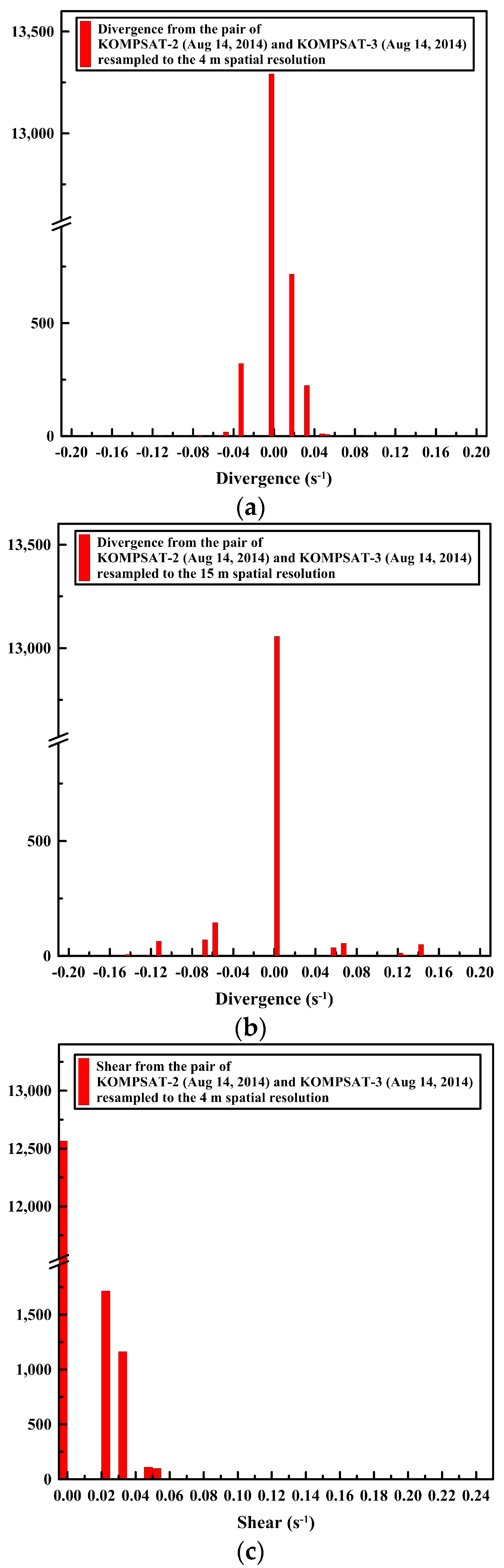
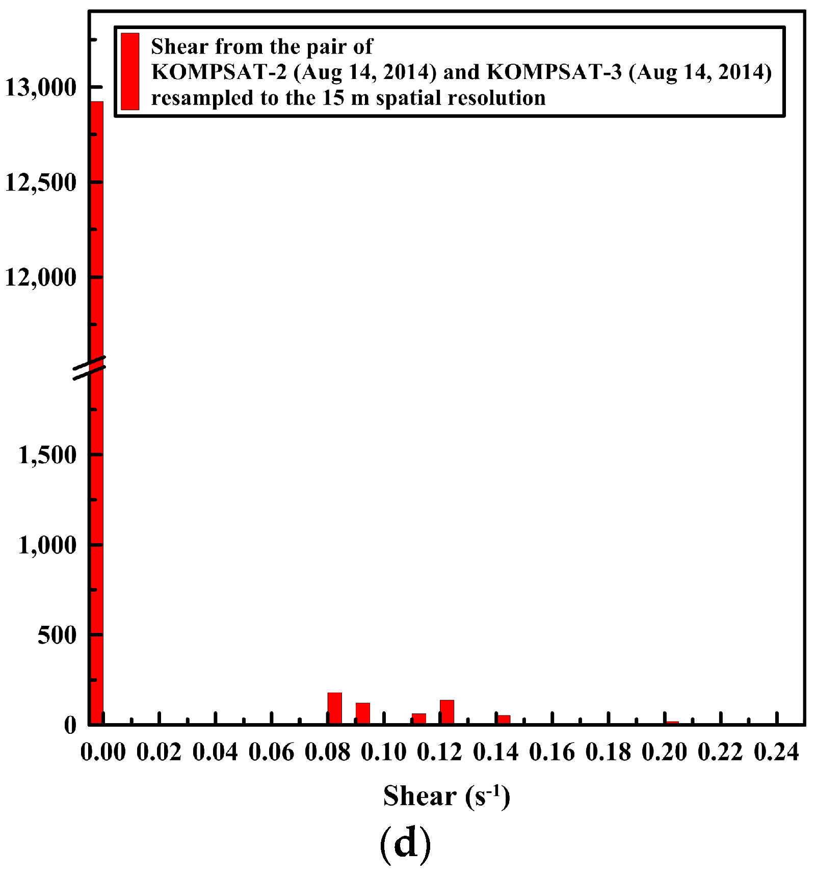
The openings and closings, and shear between the ice floes were less detectable from the image pairs resampled to the spatial resolution of 15 m compared with the image pairs of the spatial resolution of 4 m (Figure 13). The spiky peaks in the histograms of the divergence and shear from the image pairs resampled to the spatial resolution of 15 m (Figure 14b,d) became wider distributions than the histograms of the divergence and shear from the image pairs of the spatial resolution of 4 m.
5. Discussion
The results of the sea ice motion measurements illustrate that the dense distributions of the moving distance and direction from the image pairs of the 4 m spatial resolution revealed spatial patterns reflecting characteristics of sea ice motion (Figure 5). Thus, from the high-resolution satellite image-derived spatial gradient pattern of the moving distance and direction, small-scale discontinuities in motion could be visualized. For the dataset spatially resampled to 15 m, the pixel aggregation during spatial resampling smoothed the surface texture of sea ice, so that effects from small scale irregular motions, e.g., isolated drifting floe, appeared to be decreased. Increased sea ice coverage, decreased entropy and slightly more discrete colors of the motion vectors in Figure 8 when compared with Figure 5, were from a relatively increased displacement unit caused by enlarged pixel size.
The displacements of the sea ice motion varied between 409.6 and 2921.4 m for the image pairs of the spatial resolution of 4 m and between 415.0 and 2919.1 m for the image pairs of the spatial resolution of 15 m, respectively. This means that the measured sea ice motions were larger than twice of the geolocation errors of the images, i.e., minimum detectable displacement between images, approximately 100 m. Thus, the sea ice motion can be considered to be partly affected by the geolocation errors of the images. When the images partly including land area over arctic coastal region are used for coastal and land fast sea ice motion measurement, geolocation errors of satellite sensors can be decreased by assigning ground control points to accurate geographic coordinates on land area. If other high-resolution spaceborne optical sensors of higher geolocation accuracy with few meters error are applied, more accurate sea ice motion and deformation measurements can be accomplished by decreasing minimum detectable displacement.
The RMSEs and biases of the sea ice motion parameters such as displacements, directions and velocities were known to be increased in coarser resolution datasets associated with extended unit distance of the images given the errors’ dependency on the spatial resolution [17,46], and changed image texture to less sensitive conditions for precise measurement from an enlarged spatial resolution. However, results regarding the sea ice motion showed similar RMSEs and biases for both resolution datasets.
The distances between the center of the selected motion vectors from the image pair of the spatial resolution of 4 m and the center of the corresponding time-interpolated ITP80 locations varied from 17.3–69.0 m, similarly, the distances extracted from the image pairs of the spatial resolution of 15 m varied from 10.3–70.8 m. From these distance ranges varying tens of meters, the selected image-derived motion vectors of both spatial resolutions were considered to be located on the same rigid plate where ITP80 located. Thus, the differences in the RMSEs and biases between the datasets was assumed to be affected by the compound of discretization uncertainty from different pixel sizes, GPS positioning uncertainty and errors from time-interpolated ITP80. Although the pixel size was enlarged from 4 to 15 m by pixel aggregation, the RMSEs and biases of displacements, directions and velocities did not degrade distinctly.
In addition to the discretization uncertainty, possible causes of errors inducing the RMSEs and biases were GPS positioning errors in the ITP80 location records and geolocation errors of the satellite images [17]. The horizontal positioning error of GPS, e.g., the Navman Jupiter 21 GPS receiver used for some ITPs [32], is known to be 5.2 m (2d RMS) [47], and other kinds of receivers equipped in the ITPs may cause a similar number of positioning errors. The geolocation accuracy of the KOMPSAT-2 and KOMPSAT-3 satellite images assessed in December 2014 were reported as 62.8 m and 40.6 m CE90 (circular error at 90%), respectively [48]. Although the errors in the sea ice motion were combined with the GPS positioning error of the ITP80, the geolocation error of the satellite images, and measurement unit (e.g., the sliding distance of template window or pixel size) of the MCC approach, the RMSEs of the sea ice motion measurement in this study were lower than previous studies using low-resolution remote sensing datasets (e.g., about 323 m for the RGPS using 100 m spatial resolution SAR data [17] and about 3–12 km for low-resolution passive microwave data [40]).
The cross-correlation coefficient and the sea ice coverage of the image blocks from the prior image showed negative correlations as negative Kendall’s tau coefficients in the image pairs of both spatial resolutions, indicating that lower sea ice concentration was more favorable as a condition to measure precise sea ice motion in the high sea ice concentration generally in the range of 90–100% SIC from NSIDC’s passive microwave remote sensing based data as in this study (Table 6).
On the other hand, the cross-correlation coefficient and the entropy of the image blocks from the prior image showed positive correlations as positive Kendall’s tau coefficients in the image pairs of both spatial resolutions, indicating that higher complexity, i.e., combinations of smaller ice floe size, complicated boundary of ice floe, dense pressure edge and numerous melt pond, was a more favorable condition to measure precise sea ice motion (Table 6). The use of a less saturated band image also prevented the hampering of precise matching in the high sea ice concentration conditions from dimming and flattening small-scale morphological features such as the pressure edge and its shadow on the sea ice surface.
In Figure 10, Figure 11 and Figure 12, a higher entropy of the image blocks, which was a more favorable condition to measure sea ice motion using the MCC approach, was from sea ice coverages around 50%. This could be linked to the capability that enabled precise image block matching in sea ice melting season or sea ice edge area occupying a complex mixture of sea ice and open ocean using the multi-sensor high-resolution optical satellite images.
The results of the sea ice deformation measurements illustrate that prominent differences of the sea ice displacement lengths were revealed in the divergence (Figure 13a), and individual floes as unit moving plates were clearly separated by high shear (Figure 13b) from the image pairs of the 4 m spatial resolution. Thus, this small-scale deformation from high-resolution images can support understanding the interaction among individual ice floes, the aggregation of ice floes with over time, and the formation of leads or ridges [49]. Conversely, the openings and closings, and shear between the ice floes were less detectable from the image pairs resampled to the spatial resolution of 15 m (Figure 13) as the detailed ice floe moving was more homogenized from quantization to larger pixel size as quantization noise. The wider distributions of spiky peaks in the histograms of the divergence and shear in the image pairs resampled to the spatial resolution of 15 m (Figure 14) also reflect less sensitivity of deformation measurement for the enlarged pixel size, indicating discretization uncertainty [17]. Increased detection limits of deformations were also identifiable from the wider distribution of peaks in the histograms.
6. Conclusions
The feasibility of the sea ice motion measurement using the MCC technique and multi-temporal high-resolution optical satellite images from multi-sensors (which have become more available in polar regions with short acquisition time intervals) was tested. Although decreased complexity of image texture caused less favorable conditions for the MCC approach as it had overall lower cross-correlation coefficients, the sea ice motion extracted from the image pairs of the spatial resolution of 15 m yielded similar RMSEs and biases of the measurements to the image pairs resampled to the spatial resolution of 4 m as the dense motion vector field allowed the extraction of motion vectors for validations to be placed in the same rigid sea ice plate. The errors in the motion vector measurements were mainly affected by the geolocation error of the satellite images, and were improved compared with previous studies using low-resolution passive microwave or radar remote sensing datasets.
The small-scale kinematics observable from the dense sea ice motion field were affected by enlarged pixel size as the discretization uncertainty. The openings and closings between ice floes, and shear were less detectable from the image pairs resampled to the spatial resolution of 15 m, when compared with the image pairs resampled to the spatial resolution of 4 m.
Using multi-temporal high-resolution optical satellite images enabling precise image block matching (as shown in the results of this study) can be linked to the capability of specific or individual ice floe tracking that is applicable to validate wide-range sea ice motion modeling studies as a supplementary or alternative dataset to buoy based reference datasets. It has the further advantage of frequent image acquisition capability in multiple areas by means of multiple operational satellites, for example, the satellites of similar sensor characteristics such as Landsat-8 OLI and Sentinel-2; the satellites managed by same operator such as KOMPSATs; the satellites phased on the same orbit such as SPOT 6, SPOT 7, Pléiades 1A and Pléiades 1B; and identical satellites forming constellation in orbits such as RapidEye and PlanetScope. In further study, the sea ice motion and deformation measurements using high-resolution optical satellite images extending to a wider range of sea ice concentration conditions in a longer time period could expand the applicability of this approach to wider polar regions over a longer melting period.
Acknowledgments
This study was supported by the Korea Polar Research Institute (KOPRI) grant PE17120 (Research on analytical technique for satellite observation of arctic sea ice). Partial support was provided by the grant from the project titled K-AOOS (KOPRI, PM17040), funded by the Ministry of Oceans and Fisheries, Korea. The authors also gratefully acknowledge the KOMPSAT satellite images provided from the Korea Aerospace Research Institute. The ITP80 data were collected and made available by the Ice-Tethered Profiler Program based at the Woods Hole Oceanographic Institution (http://www.whoi.edu/itp).
Author Contributions
Chang-Uk Hyun conceived, designed, and performed the experiments; analyzed the results; and wrote the manuscript. Hyun-cheol Kim contributed major materials and analysis tools, and provided constructive comments on the whole manuscript.
Conflicts of Interest
The authors declare no conflict of interest.
References
- Heil, P.; Fowler, C.; Maslanik, J.; Emery, W.; Allison, I. A comparison of East Antarctic sea-ice motion derived using drifting buoys and remote sensing. Ann. Glaciol. 2001, 33, 139–144. [Google Scholar] [CrossRef]
- Emery, W.; Fowler, C.W.; Maslanik, J. Satellite-derived maps of Arctic and Antarctic sea ice motion: 1988 to 1994. Geophys. Res. Lett. 1997, 24, 897–900. [Google Scholar] [CrossRef]
- Martin, T.; Augstein, E. Large-scale drift of arctic sea ice retrieved from passive microwave satellite data. J. Geophys. Res. Oceans 2000, 105, 8775–8788. [Google Scholar] [CrossRef]
- Lavergne, T.; Eastwood, S.; Teffah, Z.; Schyberg, H.; Breivik, L.A. Sea ice motion from low-resolution satellite sensors: An alternative method and its validation in the arctic. J. Geophys. Res. Oceans 2010, 115. [Google Scholar] [CrossRef]
- Holland, P.R.; Kwok, R. Wind-driven trends in Antarctic sea-ice drift. Nat. Geosci. 2012, 5, 872–875. [Google Scholar] [CrossRef]
- Kimura, N.; Nishimura, A.; Tanaka, Y.; Yamaguchi, H. Influence of winter sea-ice motion on summer ice cover in the arctic. Polar Res. 2013, 32. [Google Scholar] [CrossRef]
- Yu, J.; Liu, A.; Yang, Y.; Zhao, Y. Analysis of sea ice motion and deformation using AMSR-E data from 2005 to 2007. Int. J. Remote Sens. 2013, 34, 4127–4141. [Google Scholar] [CrossRef]
- Emery, W.J.; Fowler, C.W.; Hawkins, J.; Preller, R.H. Fram strait satellite image-derived ice motions. J. Geophys. Res. Oceans 1991, 96, 4751–4768. [Google Scholar] [CrossRef]
- Vincent, R.; Marsden, R.; McDonald, A. Short time-span ice tracking using sequential AVHRR imagery. Atmos.-Ocean 2001, 39, 279–288. [Google Scholar] [CrossRef]
- Kwok, R. The RADARSAT geophysical processor system. In Analysis of SAR Data of the Polar Oceans; Springer: New York, NY, USA, 1998; pp. 235–257. [Google Scholar]
- Flocco, D.; Laxon, S.; Feltham, D.; Haas, C. Validation and interpretation of a new sea ice GlobIce dataset using buoys and the CICE sea ice model. In Proceedings of the EGU General Assembly, Vienna, Austria, 22–27 April 2012; p. 3174. [Google Scholar]
- Giles, A.; Massom, R.; Heil, P.; Hyland, G. Semi-automated feature-tracking of East Antarctic sea ice from Envisat ASAR imagery. Remote Sens. Environ. 2011, 115, 2267–2276. [Google Scholar] [CrossRef]
- Komarov, A.S.; Barber, D.G. Sea ice motion tracking from sequential dual-polarization RADARSAT-2 images. IEEE Trans. Geosci. Remote Sens. 2014, 52, 121–136. [Google Scholar] [CrossRef]
- Hollands, T.; Haid, V.; Dierking, W.; Timmermann, R.; Ebner, L. Sea ice motion and open water area at the Ronne Polynia, Antarctica: Synthetic aperture radar observations versus model results. J. Geophys. Res. Oceans 2013, 118, 1940–1954. [Google Scholar] [CrossRef]
- Ninnis, R.; Emery, W.; Collins, M. Automated extraction of pack ice motion from advanced very high resolution radiometer imagery. J. Geophys. Res. Oceans 1986, 91, 10725–10734. [Google Scholar] [CrossRef]
- Kwok, R.; Cunningham, G. Deformation of the arctic ocean ice cover after the 2007 record minimum in summer ice extent. Cold Reg. Sci. Technol. 2012, 76, 17–23. [Google Scholar] [CrossRef]
- Lindsay, R.; Stern, H. The RADARSAT geophysical processor system: Quality of sea ice trajectory and deformation estimates. J. Atmos. Oceanic Technol. 2003, 20, 1333–1347. [Google Scholar] [CrossRef]
- Kwok, R.; Cunningham, G.F.; Hibler, W.D. Sub-daily sea ice motion and deformation from RADARSAT observations. Geophys. Res. Lett. 2003, 30. [Google Scholar] [CrossRef]
- Hutchings, J.; Hibler, W. Small-scale sea ice deformation in the Beauport sea seasonal ice zone. J. Geophys. Res. Oceans 2008, 113. [Google Scholar] [CrossRef]
- Liu, C.-C.; Chang, Y.-C.; Huang, S.; Yan, S.-Y.; Wu, F.; Wu, A.-M.; Kato, S.; Yamaguchi, Y. Monitoring the dynamics of ice shelf margins in polar regions with high-spatial-and high-temporal-resolution space-borne optical imagery. Cold Reg. Sci. Technol. 2009, 55, 14–22. [Google Scholar] [CrossRef]
- Hagen, R.A.; Peters, M.F.; Liang, R.T.; Ball, D.G.; Brozena, J.M. Measuring arctic sea ice motion in real time with photogrammetry. IEEE Geosci. Remote Sens. Lett. 2014, 11, 1956–1960. [Google Scholar] [CrossRef]
- Kwok, R. Declassified high-resolution visible imagery for Arctic sea ice investigations: An overview. Remote Sens. Environ. 2014, 142, 44–56. [Google Scholar] [CrossRef]
- Kwok, R.; Curlander, J.C.; McConnell, R.; Pang, S.S. An ice-motion tracking system at the Alaska SAR facility. IEEE J. Ocean. Eng. 1990, 15, 44–54. [Google Scholar] [CrossRef]
- Hollands, T.; Linow, S.; Dierking, W. Reliability measures for sea ice motion retrieval from synthetic aperture radar images. IEEE J. Sel. Top. Appl. Earth Obs. Remote Sens. 2015, 8, 67–75. [Google Scholar] [CrossRef]
- Hodgson, M.E.; Kar, B. Modeling the potential swath coverage of nadir and off-nadir pointable remote sensing satellite-sensor systems. Cartogr. Geogr. Inf. Sci. 2008, 35, 147–156. [Google Scholar] [CrossRef]
- Seo, D.C.; Yang, J.Y.; Lee, D.H.; Song, J.H.; Lim, H. KOMPSAT-2 direct sensor modeling and geometric calibration/validation. In Proceedings of the International Society for Photogrammetry and Remote Sensing Congress, Beijing, China, 3–11 July 2008. [Google Scholar]
- Choi, J.; Jung, H.-S.; Yun, S.-H. An efficient mosaic algorithm considering seasonal variation: Application to KOMPSAT-2 satellite images. Sensors 2015, 15, 5649–5665. [Google Scholar] [CrossRef] [PubMed]
- Yeom, J.-M.; Hwang, J.; Jin, C.-G.; Lee, D.-H.; Han, K.-S. Radiometric characteristics of kompsat-3 multispectral images using the spectra of well-known surface tarps. IEEE Trans. Geosci. Remote Sens. 2016, 54, 5914–5924. [Google Scholar] [CrossRef]
- Cavalieri, D.; Parkinson, C.; Gloersen, P.; Zwally, H.J. Sea Ice Concentrations from Nimbus-7 SMMR and DMSP SSM/I-SSMIS Passive Microwave Data; Version 1; NASA DAAC at the National Snow and Ice Data Center: Boulder, CO, USA, 1996; Available online: http://dx.doi.org/10.5067/8GQ8LZQVL0VL (accessed on 28 March 2017).
- Overview: Ice-Tethered Profiler. Available online: http://www.whoi.edu/website/itp/ (accessed on 8 October 2016).
- Toole, J.; Krishfield, R.; Proshutinsky, A.; Ashjian, C.; Doherty, K.; Frye, D.; Hammar, T.; Kemp, J.; Peters, D.; Timmermans, M.L. Ice-tethered profilers sample the upper arctic ocean. Eos Trans. Am. Geophys. Union 2006, 87, 434–438. [Google Scholar] [CrossRef]
- Krishfield, R.; Toole, J.; Proshutinsky, A.; Timmermans, M.-L. Automated ice-tethered profilers for seawater observations under pack ice in all seasons. J. Atmos. Ocean. Technol. 2008, 25, 2091–2105. [Google Scholar] [CrossRef]
- Rösel, A.; Kaleschke, L. Comparison of different retrieval techniques for melt ponds on Arctic sea ice from Landsat and MODIS satellite data. Ann. Glaciol. 2011, 52, 185–191. [Google Scholar] [CrossRef]
- Zhang, Q.; Skjetne, R. Image techniques for identifying sea-ice parameters. Model. Identif. Control 2014, 35, 293–301. [Google Scholar] [CrossRef] [Green Version]
- Otsu, N. A threshold selection method from gray-level histograms. IEEE Trans. Syst. Man Cybern. 1979, 9, 62–66. [Google Scholar] [CrossRef]
- Gonzalez, R.C.; Woods, R.E.; Eddins, S.L. Digital Image Processing Using MATLAB; Prentice Hall: Upper Saddle River, NJ, USA, 2003; pp. 287–288. [Google Scholar]
- Kwok, R.; Schweiger, A.; Rothrock, D.; Pang, S.; Kottmeier, C. Sea ice motion from satellite passive microwave imagery assessed with ERS SAR and buoy motions. J. Geophys. Res. Oceans 1998, 103, 8191–8214. [Google Scholar] [CrossRef]
- Kwok, R. Ross sea ice motion, area flux, and deformation. J. Clim. 2005, 18, 3759–3776. [Google Scholar] [CrossRef]
- Schwegmann, S.; Haas, C.; Fowler, C.; Gerdes, R. A comparison of satellite-derived sea-ice motion with drifting-buoy data in the Weddell Sea, Antarctica. Ann. Glaciol. 2011, 52, 103–110. [Google Scholar] [CrossRef]
- Hwang, B. Inter-comparison of satellite sea ice motion with drifting buoy data. Int. J. Remote Sens. 2013, 34, 8741–8763. [Google Scholar] [CrossRef]
- Sumata, H.; Kwok, R.; Gerdes, R.; Kauker, F.; Karcher, M. Uncertainty of Arctic summer ice drift assessed by high-resolution SAR data. J. Geophys. Res. Oceans 2015, 120, 5285–5301. [Google Scholar] [CrossRef]
- Notarstefano, G.; Poulain, P.-M.; Mauri, E. Estimation of surface currents in the Adriatic sea from sequential infrared satellite images. J. Atmos. Ocean. Technol. 2008, 25, 271–285. [Google Scholar] [CrossRef]
- Stern, H.L.; Moritz, R.E. Sea ice kinematics and surface properties from RADARSAT synthetic aperture radar during the SHEBA drift. J. Geophys. Res. Oceans 2002, 107. [Google Scholar] [CrossRef]
- Yau, C. R Tutorial with Bayesian Statistics Using OpenBUGS. 2012. Available online: http://www.r-tutor.com/content/r-tutorial-ebook (accessed on 16 March 2017).
- Kwok, R. Satellite remote sensing of sea-ice thickness and kinematics: A review. J. Glaciol. 2010, 56, 1129–1140. [Google Scholar] [CrossRef]
- Tschudi, M.; Fowler, C.; Maslanik, J.; Stroeve, J. Tracking the movement and changing surface characteristics of Arctic sea ice. IEEE J. Sel. Top. Appl. Earth Obs. Remote Sens. 2010, 3, 536–540. [Google Scholar] [CrossRef]
- Centurioni, L. Observations of large-amplitude nonlinear internal waves from a drifting array: Instruments and methods. J. Atmos. Ocean. Technol. 2010, 27, 1711–1731. [Google Scholar] [CrossRef]
- SIIS (SI Imaging Services). Location Accuracy of KOMPSAT Products: DEC. 2014. Available online: http://www.si-imaging.com/lfile/Geolocation (accessed on 3 August 2016).
- Kwok, R.; Sulsky, D. Arctic Ocean sea ice thickness and kinematics: Satellite retrievals and modeling. Oceanography 2010, 23, 134–143. [Google Scholar] [CrossRef]
Figure 1.
Overview of satellite image acquisition and ITP80 buoy deployment: (a) schematic placements of satellite images used to measure sea ice motion and deformation, and synoptic trajectory of the ITP80; and (b) a view of the ice floe where the ITP80 was deployed from the Korean icebreaker research vessel (IBRV) Araon, captured by the KOMPSAT-3 satellite on 11 August 2014.


Figure 2.
Sea ice condition in the study area: (a) the sea ice concentration (SIC) around the study area retrieved from the daily SIC data of the National Snow and Ice Data Center (NSIDC) from Nimbus-7 SMMR and DMSP SSM/I-SSMIS Passive Microwave Data [29] on 14 August 2014; and (b) an overview of sea ice coverage captured in each satellite image.


Figure 3.
Working processes for sea ice motion and deformation measurements.

Figure 4.
The histogram of the cross-correlation coefficient: (a) the image pairs of the spatial resolution of 4 m; and (b) the image pairs of the spatial resolution of 15 m.
Figure 4.
The histogram of the cross-correlation coefficient: (a) the image pairs of the spatial resolution of 4 m; and (b) the image pairs of the spatial resolution of 15 m.
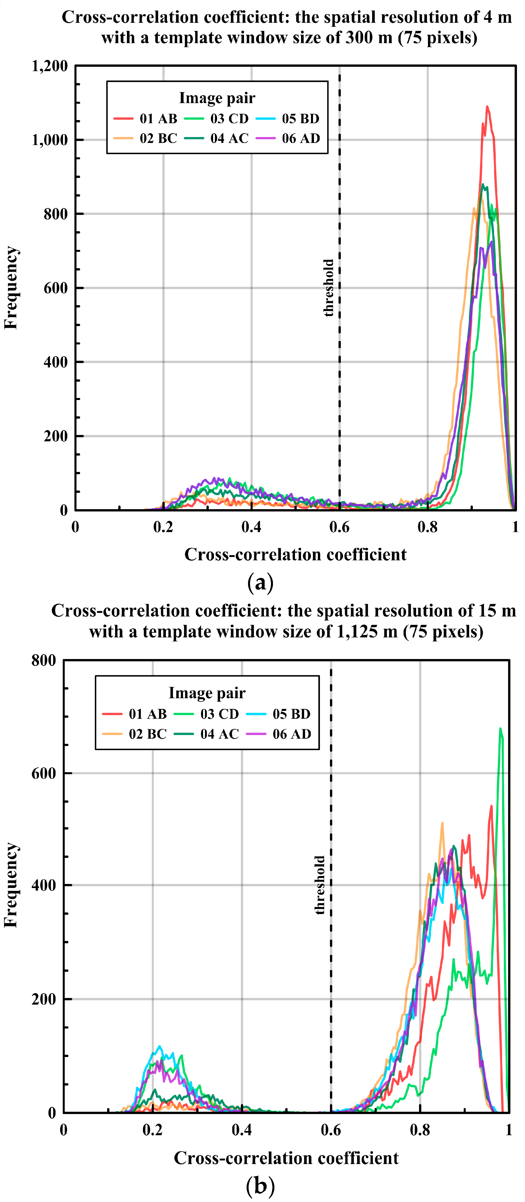
Figure 5.
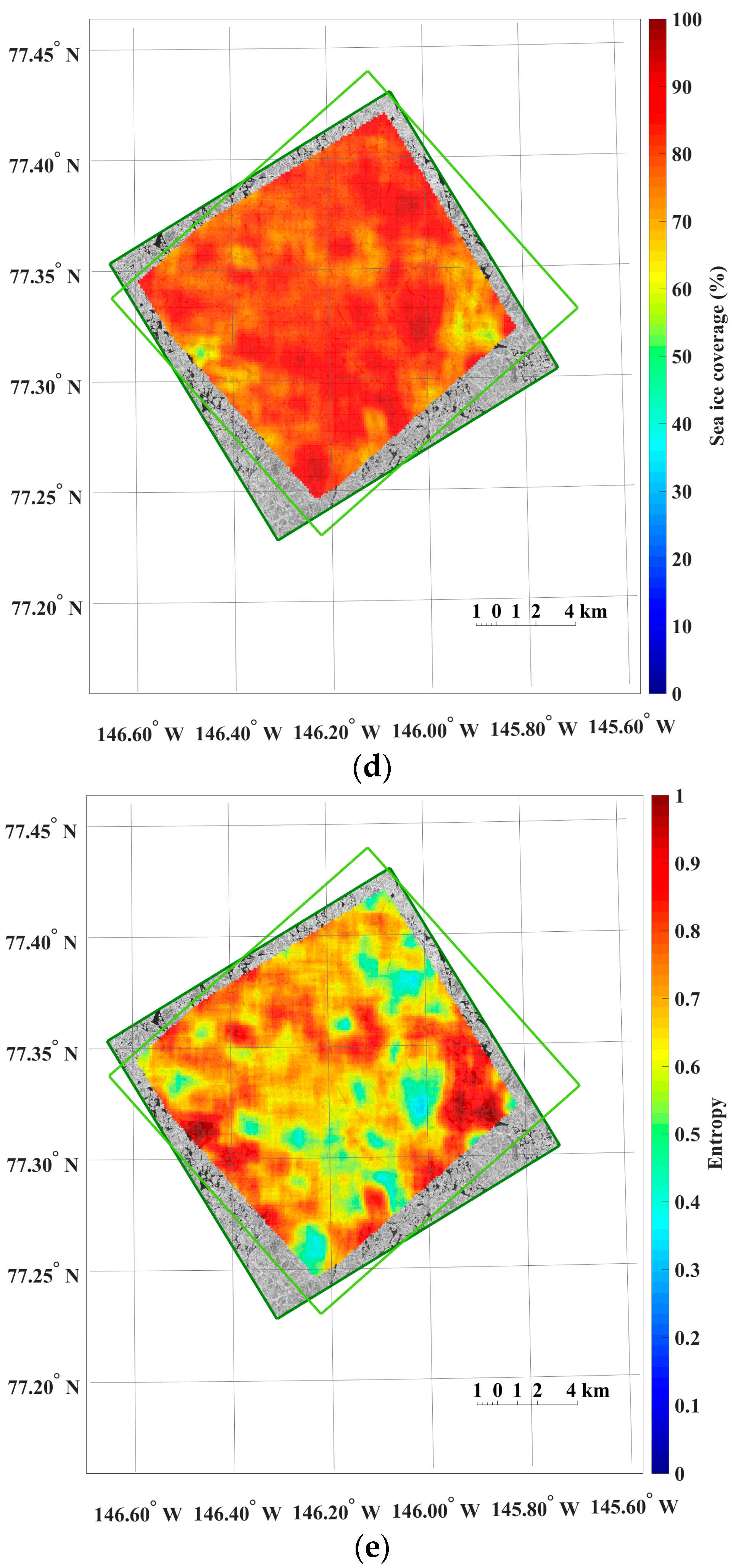
An example of the results from sea ice motion measurement using the KOMPSAT-2 image acquired on 14 August 2014 (i.e., prior image) and the KOMPSAT-3 image acquired on 14 August 2014 (i.e., posterior image), resampled to the spatial resolutions of 4 m: (a) magnitudes of the sea ice motion vectors; (b) directions (headings) of the sea ice motion vectors, measured counterclockwise from east; (c) cross-correlation coefficient of each image block; (d) sea ice coverage of each image block in the prior image; and (e) entropy of each image block in the prior image, plotted only for the image blocks after applying the cross-correlation coefficient threshold and outlier removal.
Figure 5.
An example of the results from sea ice motion measurement using the KOMPSAT-2 image acquired on 14 August 2014 (i.e., prior image) and the KOMPSAT-3 image acquired on 14 August 2014 (i.e., posterior image), resampled to the spatial resolutions of 4 m: (a) magnitudes of the sea ice motion vectors; (b) directions (headings) of the sea ice motion vectors, measured counterclockwise from east; (c) cross-correlation coefficient of each image block; (d) sea ice coverage of each image block in the prior image; and (e) entropy of each image block in the prior image, plotted only for the image blocks after applying the cross-correlation coefficient threshold and outlier removal.
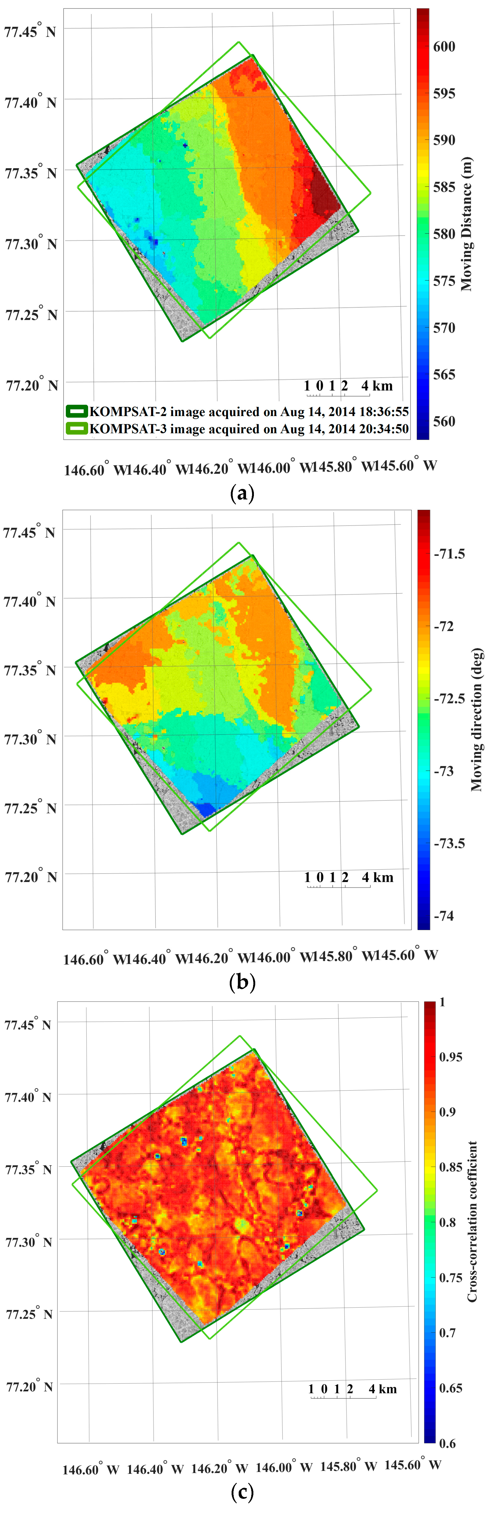

Figure 6.
An example of the matched image block with the cross-correlation coefficient of 0.539, lower than the threshold value (i.e., the cross-correlation coefficient = 0.6), retrieved from: (a) the KOMPSAT-2 image acquired on 14 August 2014 (i.e., prior image); and (b) the KOMPSAT-3 image acquired on 14 August 2014 (i.e., posterior image), resampled to the spatial resolutions of 4 m.

Figure 7.
Wind speed and direction, of which the wind originates, measured in the IBRV Araon during the image acquisition period, refined by 10 s moving average. The A, B, C and D denote the image acquisition times.
Figure 7.
Wind speed and direction, of which the wind originates, measured in the IBRV Araon during the image acquisition period, refined by 10 s moving average. The A, B, C and D denote the image acquisition times.

Figure 8.
The results from sea ice motion measurement using the same image pair as Figure 5, resampled to the spatial resolutions of 15 m: (a) magnitudes of the sea ice motion vectors; (b) directions (headings) of the sea ice motion vectors, measured counterclockwise from east; (c) cross-correlation coefficient of each image block; (d) sea ice coverage of each image block in the prior image; and (e) entropy of each image block in the prior image, plotted only for the image blocks after applying the cross-correlation coefficient threshold without additional outlier removal.
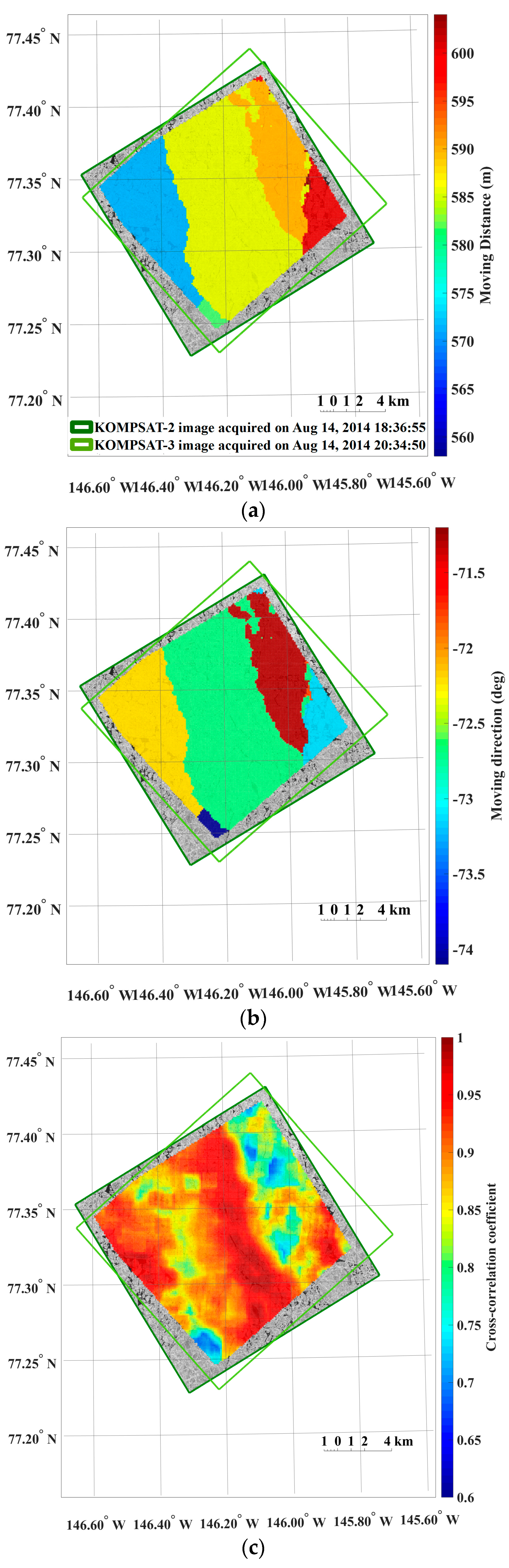

Figure 9.
Comparison between sea ice drifts measured from sequential satellite image pairs and ITP80 track records: (a) displacements; (b) directions; and (c) velocities.
Figure 9.
Comparison between sea ice drifts measured from sequential satellite image pairs and ITP80 track records: (a) displacements; (b) directions; and (c) velocities.

Figure 10.
The relationships (Kendall’s tau coefficient) between the cross-correlation coefficient and sea ice image properties using the same image pairs as Figure 5 and Figure 8: (a) cross-correlation coefficient vs. sea ice coverage of the image blocks from the prior image of the spatial resolutions of 4 m; (b) cross-correlation coefficient vs. entropy of the image blocks from the prior image of the spatial resolutions of 4 m; (c) cross-correlation coefficient vs. sea ice coverage of the image blocks from the prior image of the spatial resolutions of 15 m; and (d) cross-correlation coefficient vs. entropy of the image blocks from the prior image of the spatial resolutions of 15 m.


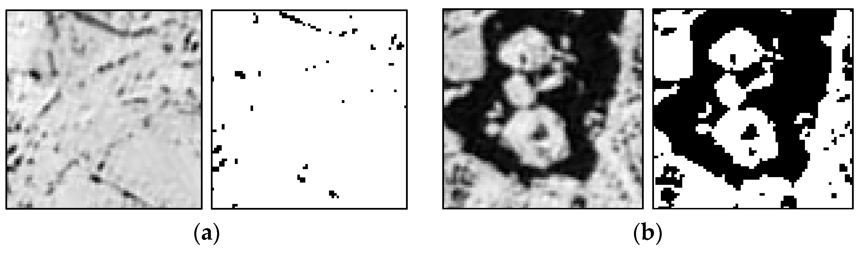
Figure 11.
Examples of the sea ice coverage and entropy of the matched block (75 × 75 pixels equivalent to 300 × 300 m) from the KOMPSAT-2 image acquired on 14 August 2014 (i.e., prior image) and the KOMPSAT-3 image acquired on 14 August 2014 (i.e., posterior image), resampled to the spatial resolution of 4 m: (a) 14 bit grey scale image block and binarized sea ice image block showing the maximum sea ice coverage parameter (97.849) and 3rd lowest entropy (0.150) of the prior image; and (b) 14 bit grey scale image block and binarized sea ice image block showing the maximum entropy (1.000) and the sea ice coverage parameter around 50% (50.08) of the prior image. The image blocks were chosen from the blocks designated as the cross-correlation coefficients higher than 0.6, and after additional outlier removal.

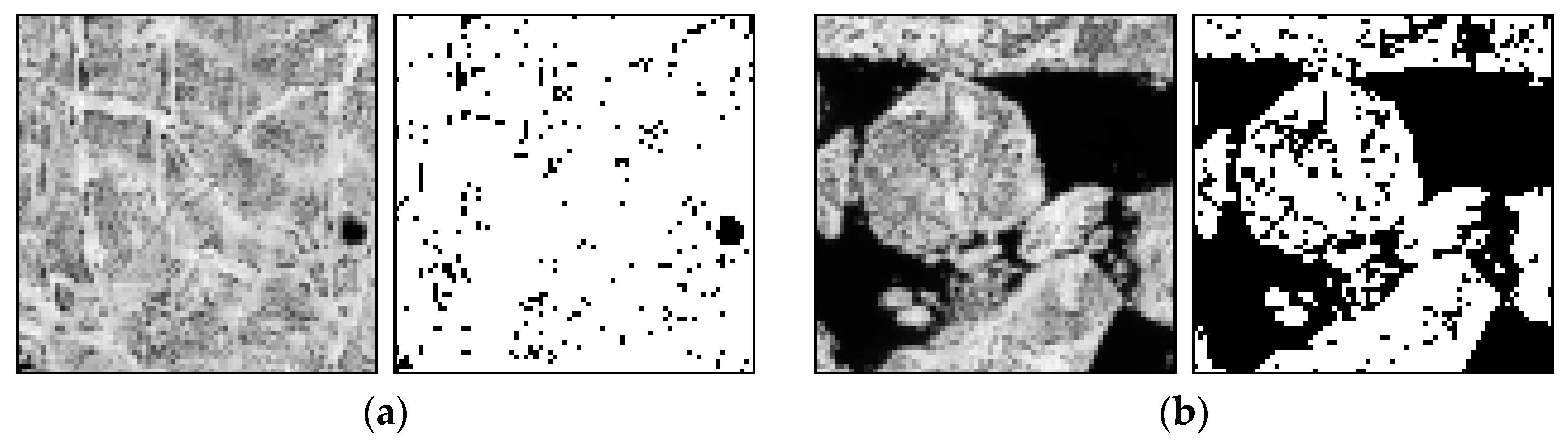
Figure 12.
The sea ice coverage and entropy of the matched block (75 × 75 pixels equivalent to 1125 × 1125 m) from the same image pair of Figure 11, resampled to the spatial resolution of 15 m: (a) 14 bit grey scale image block and binarized sea ice image block showing the maximum sea ice coverage parameter (93.938) and minimum entropy (0.330) of the prior image; and (b) 14 bit grey scale image block and binarized sea ice image block showing the minimum sea ice coverage parameter around 50% (51.236) and maximum entropy (1.000) of the prior image. The image blocks were chosen from the blocks designated as the cross-correlation coefficients higher than 0.6.

Figure 13.
An example of the sea ice deformation using the KOMPSAT-2 image acquired on 14 August 2014 (i.e., prior image) and the KOMPSAT-3 image acquired on 14 August 2014 (i.e., posterior image: (a) divergence and (b) shear from the image pair resampled to the spatial resolutions of 4 m; and (c) divergence and (d) shear from the image pair resampled to the spatial resolutions of 15 m.


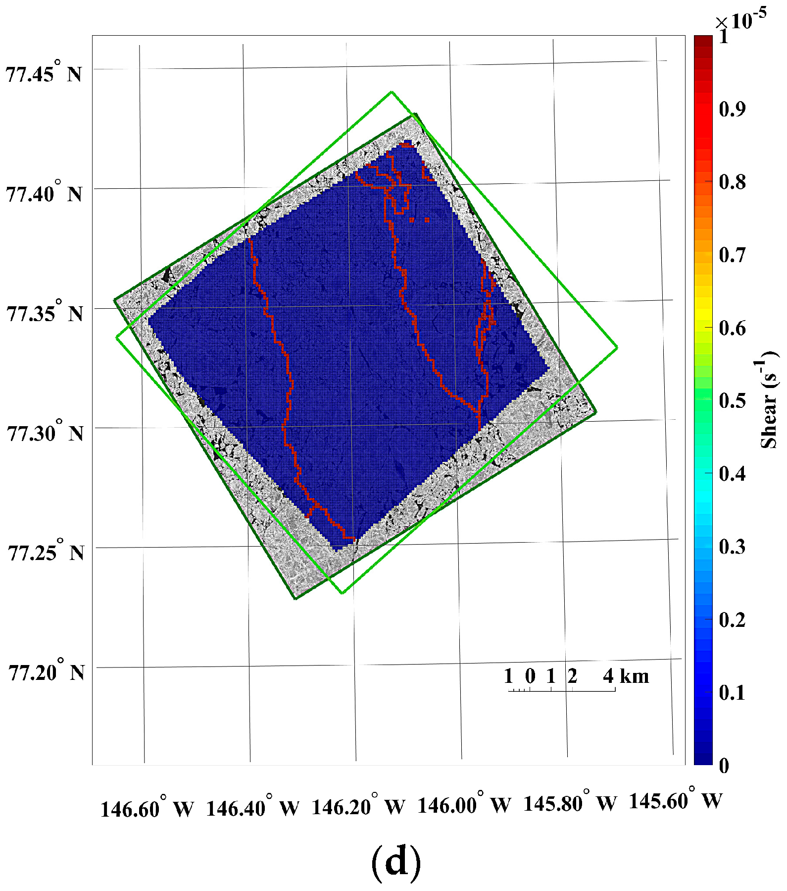
Figure 14.
The histogram of the sea ice deformation using the same image pair with Figure 13: the histograms of divergence from (a) the image pair resampled to the spatial resolutions of 4 m; and (b) the same image pair resampled to the spatial resolutions of 15 m, and the histograms of shear from (c) the image pair resampled to the spatial resolutions of 4 m; and (d) the same image pair resampled to the spatial resolutions of 15 m.


Table 1.
Specifications of the Korea Multi-Purpose Satelllite-2 (KOMPSAT-2) and Korea Multi-Purpose Satelllite-3 (KOMPSAT-3) satellites and imaging sensors [26,27,28].
| KOMPSAT-2 | KOMPSAT-3 | |
|---|---|---|
| Date of launch | 28 July 2006 | 17 May 2012 |
| Main payload | MSC (Multispectral Camera) | AEISS (Advanced Earth Imaging Sensor System) |
| Orbit height | 685 km | 685 km |
| Spatial resolution | 1.0 m Pan and 4.0 m MS | 0.7 m Pan and 2.8 m MS |
| Spectral bands | 500–900 nm PAN | 450–900 nm PAN |
| 450–520 nm MS1 (blue) | 450–520 nm MS1 (blue) | |
| 520–600 nm MS2 (green) | 520–600 nm MS2 (green) | |
| 630–690 nm MS3 (red) | 630–690 nm MS3 (red) | |
| 760–900 nm MS4 (NIR) | 760–900 nm MS4 (NIR) | |
| Mean local time on ascending node | 10:50 h | 13:30 h |
| Data quantization | 10 bit | 14 bit |
| Swath width | 15 km | 16 km |
Table 2.
Details for satellite image acquisition.
| ID | Satellite Image | Acquisition Date and Time (UTC) |
|---|---|---|
| A | KOMPSAT-2 MSC | 14 August 2014 18:36:55 |
| B | KOMPSAT-3 AEISS | 14 August 2014 20:34:50 |
| C | KOMPSAT-2 MSC | 15 August 2014 17:37:46 |
| D | KOMPSAT-3 AEISS | 15 August 2014 21:13:14 |
Table 3.
Details for the ITP80 deployment and location record.
| ITP80 | Specifications |
|---|---|
| Deployed date | 12 August 2014 |
| Deployed location | 77°24.2′N, 146°10.3′W |
| Localization method | GPS positioning |
| Location measurement | Hourly |
| Data processing level | Level 3 |
Table 4.
Combinations of image pair for measuring and validating sea ice motion.
| Image Pair | Time Interval (hh:mm:ss) | |
|---|---|---|
| 1 | KOMPSAT-2 (14 August 2014)–KOMPSAT-3 (14 August 2014) | 01:57:55 |
| 2 | KOMPSAT-3 (14 August 2014)–KOMPSAT-2 (15 August 2014) | 21:02:56 |
| 3 | KOMPSAT-2 (15 August 2014)–KOMPSAT-3 (15 August 2014) | 03:35:28 |
| 4 | KOMPSAT-2 (14 August 2014)–KOMPSAT-2 (15 August 2014) | 23:00:51 |
| 5 | KOMPSAT-3 (14 August 2014)–KOMPSAT-3 (15 August 2014) | 24:38:24 |
| 6 | KOMPSAT-2 (14 August 2014)–KOMPSAT-3 (15 August 2014) | 26:36:19 |
Table 5.
Quality assessment of the sea ice motion measurement by comparing the image-derived motion vectors with the motions connecting the time-interpolated buoy locations.
Table 5.
Quality assessment of the sea ice motion measurement by comparing the image-derived motion vectors with the motions connecting the time-interpolated buoy locations.
| Dataset | Parameter | RMSE | Bias |
|---|---|---|---|
| Spatial resolution of 4 m | Displacement | 57.7 m | –11.4 m |
| Velocity | 19.0 m·h−1 | –4.6 m·h−1 | |
| Direction | 4.0° | –1.5° | |
| Spatial resolution of 15 m | Displacement | 60.7 m | –13.5 m |
| Velocity | 18.7 m·h−1 | –4.3 m·h−1 | |
| Direction | 3.8° | –2.0° |
Table 6.
The relationships between cross-correlation coefficient and sea ice image properties.
| Image Pair | Correlation Coefficient (Tau) | |||
|---|---|---|---|---|
| Spatial Resolution of 4 m | Spatial Resolution of 15 m | |||
| Cross-Correlation Coefficient vs. Sea Ice Coverage | Cross-Correlation Coefficient vs. Entropy | Cross-Correlation Coefficient vs. Sea Ice Coverage | Cross-Correlation Coefficient vs. Entropy | |
| 1 | −0.341 | 0.338 | −0.221 | 0.222 |
| 2 | −0.200 | 0.195 | −0.166 | 0.166 |
| 3 | −0.287 | 0.277 | −0.026 | 0.026 |
| 4 | −0.233 | 0.230 | −0.193 | 0.193 |
| 5 | −0.121 | 0.116 | −0.236 | 0.237 |
| 6 | −0.235 | 0.231 | −0.258 | 0.258 |
© 2017 by the authors. Licensee MDPI, Basel, Switzerland. This article is an open access article distributed under the terms and conditions of the Creative Commons Attribution (CC BY) license (http://creativecommons.org/licenses/by/4.0/).
Share and Cite
MDPI and ACS Style
Hyun, C.-U.; Kim, H.-c. A Feasibility Study of Sea Ice Motion and Deformation Measurements Using Multi-Sensor High-Resolution Optical Satellite Images. Remote Sens. 2017, 9, 930. https://doi.org/10.3390/rs9090930
AMA Style
Hyun C-U, Kim H-c. A Feasibility Study of Sea Ice Motion and Deformation Measurements Using Multi-Sensor High-Resolution Optical Satellite Images. Remote Sensing. 2017; 9(9):930. https://doi.org/10.3390/rs9090930
Chicago/Turabian StyleHyun, Chang-Uk, and Hyun-cheol Kim. 2017. "A Feasibility Study of Sea Ice Motion and Deformation Measurements Using Multi-Sensor High-Resolution Optical Satellite Images" Remote Sensing 9, no. 9: 930. https://doi.org/10.3390/rs9090930
Note that from the first issue of 2016, this journal uses article numbers instead of page numbers. See further details here.