Environmental Variability and Oceanographic Dynamics of the Central and Southern Coastal Zone of Sonora in the Gulf of California

Abstract

This study analyzed monthly and inter-annual variability of mesoscale phenomena, including the El Niño Southern Oscillation (ENSO), the Pacific Decadal Oscillation (PDO) climate indexes and wind intensity considering their influence on sea surface temperature (SST) and chlorophyll a (Chl-a). These analyses were performed to determine the effects, if any, of climate indexes and oceanographic and environmental variability on the central and southern coastal ecosystem of Sonora in the Gulf of California (GC). Monthly satellite images of SST (°C) and Chl-a concentration were used with a 1-km resolution for oceanographic and environmental description, as well as monthly data of the climate indexes and wind intensity from 2002–2015. Significant differences (p > 0.05) were observed while analyzing the monthly variability results of mesoscale phenomena, SST and Chl-a, where the greatest percentage of anti-cyclonic gyres and filaments was correlated with a greater Chl-a concentration in the area of study, low temperatures and, thus, greater productivity. Moreover, the greatest percentage of intrusion was correlated with the increase in temperature and cyclonic gyres and a strong decrease of Chl-a concentration values, causing oligotrophic conditions in the ecosystem and a decrease in upwelling and filament occurrence. As for the analysis of the interannual variability of mesoscales phenomena, SST, Chl-a and winds, the variability between years was not significant (p > 0.05), so no correlation was observed between variabilities or phenomena. The results of the monthly analyses of climate indexes, environmental variables and wind intensity did not show significant differences for the ENSO and PDO indexes (p > 0.05). Nonetheless, an important correlation could be observed between the months of negative anomalies of the ENSO with high Chl-a concentration values and intense winds, as well as with low SST values. The months with positive ENSO anomalies were correlated with high SST values, low Chl-a concentration and moderate winds. Significant inter-annual differences were observed for climate indexes where the years with high SST values were related to the greatest positive anomaly of ENSO, of which 2002 and 2009 stood out, characterized as moderate Niño years, and 2015 as a strong El Niño year. The years with the negative ENSO anomaly were related to the years of lower SST values, of which 2007–2008 and 2010–2011 stood out, characterized as moderate Niñas. Thus, variability associated with mesoscale oceanographic phenomena and seasonal and inter-annual variations of climate indexes had a great influence on the environmental conditions of the coastal ecosystem of Sonora in the Gulf of California.

1. Introduction

The Gulf of California (GC), one of the 24 marginal seas, one of the five largest gulfs of the Pacific Ocean [1] and considered one of the most productive seas of the planet [2,3], shows two periods separated by two short transition phases, a cold one with high biological productivity and a warm one with low productivity, attributed to mesoscale processes, such as thermocline, surface circulation induced by the wind, gyres, filaments and upwelling [4,5]. These mesoscale processes are the result of atmospheric forcing (wind) interaction in the eastern border of the Pacific, inducing a significant (barotropic) variability of eddy kinetic energy, which is associated with current forcing fluctuations in most regions [6,7].

The central region of the GC has intense seasonal upwelling, which takes place from January–April and from November–December [8,9]. The surface circulation pattern is influenced by seasonal winds with a flux toward the south in winter and toward the north in summer with important differences in temperature between both periods [10,11,12,13,14]. High temperatures and oligotrophic characteristics are generated during the summer with the arrival of the Mexican Coastal Current (MCC) intrusion to the area of study, generating a cyclonic circulation in this zone [13,15], while wind forcing in the winter generates filaments of cold water associated with high chlorophyll a (Chl-a) concentrations; likewise, cyclonic gyres (with counterclockwise circulation in the Northern Hemisphere) are responsible for the dispersion of high Chl-a concentration [16,17].

These oceanographic conditions of the GC vary in a wide interval of spatial scales (from a few to hundreds of km) and of temporal scales (monthly, seasonal, annual and inter-annual to decadal), exerting an influence on marine ecosystems and providing biologically-rich and productive habitats for a great diversity of ecologically- and commercially-important species [18,19,20,21,22]. These enriching processes of nutrient upwelling and mixing affect the trophic network, while the processes of particle concentration (gyres and currents) generate favorable conditions for spawning, survival and larval dispersion of phytoplankton organisms [14,23,24,25,26].

Many large-scale phenomena that act on varied time scales from the El Niño-Southern Oscillation (ENSO) occur in the Pacific Ocean with month-year cycles from decadal to multi-decadal frequency events, such as the Pacific Decadal Oscillation (PDO). Their effects are detectable from global to local ecosystems, and their aggregate contributions establish climate shifts that have shown fluctuations in atmospheric and oceanic conditions, such as sea temperature [27], wind fields associated with atmospheric pressure variations [28], ocean currents [29], coastal upwelling [30] and mixed layer depths [31]. Many of these climate variations occur via atmospheric-oceanic teleconnections [32], which extend from the troposphere to the ocean surface, including fluctuations in sea level pressure that are closely linked to changes in surface winds, sea surface temperature (SST), heat content, mixed layer and thermocline depth. Climate variability receives considerable attention because of large-scale influences in the North Pacific due to their impact on tropical and extra-tropical climate [33] and weather over North America [34].

The El Niño Southern Oscillation, perhaps the most studied large-scale phenomenon, comprises two phases. The warm El Niño phase, which has been studied extensively in the Pacific Ocean [12,32], is characterized by the weakening of trade winds, warming the sea surface layer in the tropical-subtropical eastern Pacific, a switch from low to high atmospheric pressure near Darwin, Australia, and the opposite effect near the Tahiti Islands, where it is termed the Southern Oscillation. The La Niña cold phase of ENSO is much less studied in the Pacific. It is characterized by an intensification of trade winds, cooling the sea surface layer in the tropical-sub-tropical Eastern Pacific, very low atmospheric pressure near Darwin, Australia, and very high pressure near the Tahiti Islands [35,36].

The Pacific Decadal Oscillation, another large-scale phenomenon, is a pattern of ocean variability over the entire Pacific, similar to ENSO in some respects, but with a much longer cycle [37,38]. It is also defined by two phases; the positive phase in the North Pacific occurs when SST anomalies are cold in the central North Pacific and warm along the Pacific coast and when sea level pressure is below average in the North Pacific [39], while the converse occurs during the negative phase. Both phases are calculated by the standardized difference between SSTs in the north-central Pacific and Gulf of Alaska. The PDO phases may be important in enhancing or dampening ENSO impacts [40].

The Pacific Ocean exerts a strong influence over the oceanographic conditions of the Gulf of California because of its connection to the eastern tropical Pacific [4]. The dynamic forcing from the Pacific over the gulf is one of the most important oceanographic features because it integrates relevant phenomena, such as salt and heat, global balances, thermohaline circulation and barotropic ocean circulation [12,41].

Studies have demonstrated the effects of these large-scale phenomena on the Gulf of California region, and satellite analyses have shown the influence of ENSO over SST variability. Based on satellite records of SST anomalies [11,42], it has been shown that temperature in the gulf registered up to 3 °C above normal during El Niño, while it was up to 3 °C below normal during La Niña.

Similarly, studies on the PDO have shown its influence on pressure, wind, temperature and precipitation patterns of the North Pacific [37,43,44]. Its temporal modulations are linked to several important biological and ecosystem variables in the ocean [45,46]. Nevertheless, other parameters, such as decadal fluctuations in salinity, nutrients and Chl-a in the eastern North Pacific, are often poorly correlated with the PDO [47].

The GC is complex in terms of climate variability in different time scales (ENSO), decadal to interdecadal and long-term trend besides the influence of climate change (CC) in the long-term trend [48] affecting marine communities [49,50]. It is located in the transition zone between the tropical and subtropical climate regimes and exposed to natural variability modes at a large scale, as ENSO, PDO and their spatial-temporal interactions [51]; in addition to the previous effects, this environmental variability causes changes in the limits of species distribution; mismatches between predators and prey; massive mortality events; and the increase of diseases, which are some of the biological effects attributed to CC [50,52]. Moreover, impacts in the GC ecosystem are caused by harmful algal blooms, deterioration in the mangrove area and morphology besides changes in hydrographic conditions in the coastal zone affecting aquaculture, mortality and changes in the distribution of benthic communities and important species for fisheries [53].

Because the GC remains free of clouds most of the year, this region is ideal for using high-resolution satellite-derived data to study surface variability and climate effects on some variables, such as SST and Chl-a. These effects have been well documented in the GC with more than three decades of satellite measurements (1980–2015). Soto-Mardones et al. [11], Lavín et al. [42] and Herrera-Cervantes et al. [13] examined high-resolution satellite-derived SST and chlorophyll data and their relationships to ENSO spatial signatures for different periods (1984–2004 and 1997–2006 respectively); they found that ENSO is the most important inter-annual variability signal. Kahru et al. [54], based on satellite data from the Ocean Color Temperature Scanner (OCTS), Sea-viewing Wide Field-of-view Sensor (SeaWiFS), the Moderate Resolution Imaging Spectroradiometer (MODIS-Aqua and MODIS-Terra), the Advanced Very-High-Resolution Radiometer (AVHRR) and the Vertically Generalized Production Model (VGPM) primary productivity model, found that the semiannual cycle of surface Chl-a concentration was higher during the spring and fall transition periods when the GC surface circulation was switching between cyclonic gyres in the summer and anti-cyclonic gyres in the winter. Satellite images, jointly with hydrographic surveys, suggest that the mesoscale variability in the GC is characterized by a complex pattern of filaments, meanders and semi-permanent eddy structures. These events carry organisms and properties from the entrance to the whole length of the GC [14], which cause important seasonal variability in the mean field of variables, such as SST and Chl-a, impacting the GC ecosystem, one of the most diverse marine biological communities in the world and a strategic region for marine fisheries in Mexico, ideal for the use of SST and Chl-a satellite images for its environmental characterization.

Therefore, the objective of this work was to perform a temporal-spatial characterization of the mesoscale processes and their relationships with the variations of SST and Chl-a concentration using high-resolution satellite-derived MODIS data. The influence of ENSO and PDO signals on SST, Chl-a and wind variations, as well as their influence on the coastal ecosystem of Sonora in the GC are included in the analysis.

2. Materials and Methods

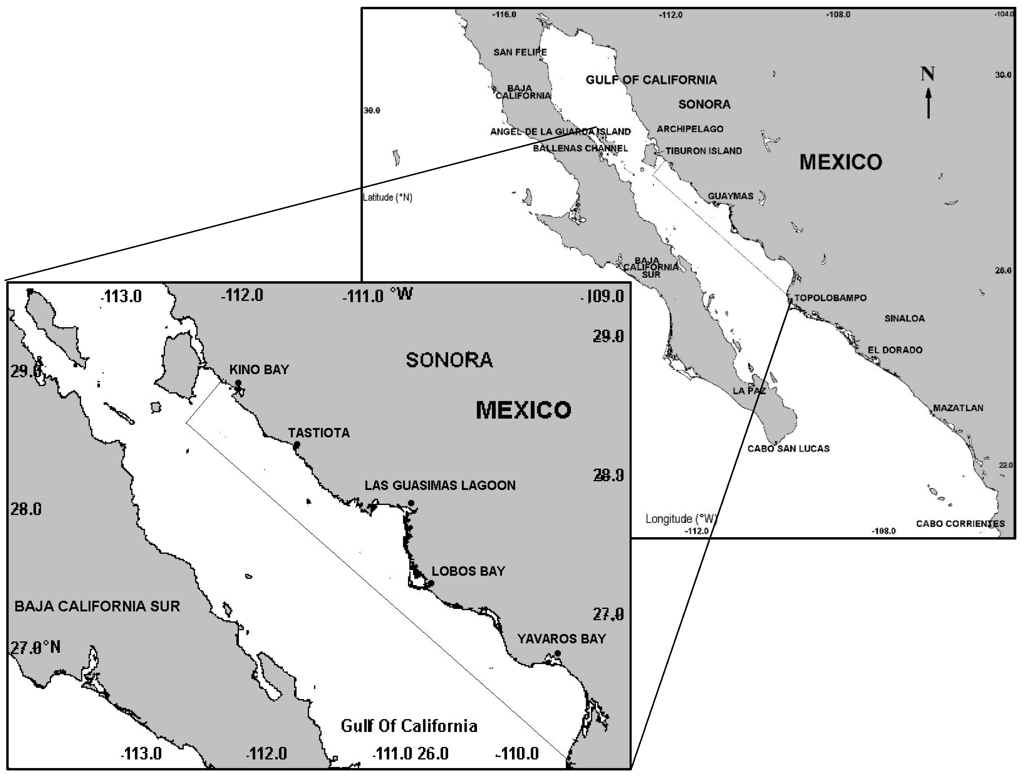
2.1. Study Area

This study comprised the central and southern coastal regions of Sonora, Mexico, in the GC (from Bahía Kino to Yavaros, Sonora (Figure 1)), with several sub-basins, low tide amplitude, high productivity in winter due to coastal upwelling processes associated with winter wind patterns [8,9] and low productivity during the summer causing oligotrophic conditions [2,55]. Important differences in SST have been reported in the zone from winter to summer [11], as well as an important generation of cyclonic and anti-cyclonic gyres occupying the entire width of the GC [2,56].

2.2. Environmental Characterization and Oceanographic Dynamics

For spatial-temporal environmental characterization and oceanographic dynamics analyses, monthly averaged composite images of SST (°C) and Chl-a (mg/m³) were used with a spatial resolution of 1 km, produced by Dr. Mati Kahru (Scripps Institution of Oceanography, http://www.wimsoft.com/CAL/). To produce monthly composite images, Kahru et al. (2012) processed and averaged daily images of SST and Chl-a Level-2 and unmapped datasets from multiple sensors: SeaWiFS, MODIS-Terra and MODIS-Aqua, MERIS (Medium Spectral Resolution Imaging Spectrometer) and VIIRS (Visible and Infrared Imager/Radiometer Suite) downloaded from the NASA’s Ocean Color website (https://oceancolor.gsfc.nasa.gov/). Individual swaths were mapped to a common projection using an Albers Conic Equal Area projection to make each one comparable; because of the Earth’s curvature, the viewing geometry is different for each pixel, and the ground projection of each satellite swath is also different. Cloud-free pixels from many satellite passes were merged to create composite images. As clouds move around during the day, it is possible to use holes in the clouds and composite data from multiple sensors and multiple overpasses during the day to get maximum coverage. Merging data from multiple sensors has improved spatial and temporal coverage compared to a single sensor and correspondence to in situ data because of regional optimization [57]. Sub-images of 1438 × 1397 pixels were cut for the gulf from the supplied images, and mean Chl-a and SST for each month were calculated using routines included in the Windows Image Manager Automation Module software (WIM/WAM) [58].

Satellite data were processed by Mati Karhu (www.wimsoft.com/Satellite_Projects.htm), who grouped them for the region of the California Current and at the same time included the region of the Gulf of California by using two types of measurements: sea surface temperature (SST) and superficial chlorophyll a concentration (Chl-a). In case they are required, other variables can be added, such as the diffuse attenuation of downwelling light at 490 nm (Kd490) and the remote sensing reflectances at various wavelengths (e.g., Rrs443, Rrs490, Rrs555, and so on).

For each year, these data are composed of different time intervals: day, 5 days, 15 days, month (www.wimsoft.com/CAL/). Likewise, if possible, similar data of different sensors are merged to increase coverage and reduce lost data due to clouds.

The set of high-resolution data (1 km) of SST and Chl-a with numerical values are in HDF4 and PNG format, which can be read by different image-processing programs where the attributes within the HDF files provide information on the same data. The complete resulting image is 3840 pixels wide and 3405 pixels high. Image annotations are reduced four times and include longitude/latitude grid, etc., so special care should be taken while interpreting pixel value. The corresponding latitudes and longitudes of each pixel can be obtained from the HDF4 file (spg.ucsd.edu/Satellite_Data/California_Current/cal_aco_3840_Latitude_Longitude.hdf).

The SST and Chl-a products are simple averages of all valid data of all of the sensors available: MODIST and MODISA for SST; sensors such as MODIST, MODISA, MERIS and VIIRS for Chl-a. Not all sensors are always available. The most advanced data merging is described in Kahru et al. (2012, 2015, 2016). Both SST and Chl-a values in the HDF files use 1 byte per pixel with specific scaling.

Linear scaling is used for SST and logarithmic scaling for Chl-a. The scaling equations using the pixel value (PV) as the unsigned byte (from 0–255) are: SST (deg C) = 0.15 × PV − 3.0 and to Chl (mg m⁻³) = 10^(0.015 × PV − 2.0), i.e., 10 to the power of 0.015 × PV − 2.0. Pixel values of 0 and 255 (and the corresponding scaled values) are considered invalid and must be excluded in any statistics (www.wimsoft.com/CAL/).

Additionally, a database was built for an area centered at Guaymas basin (27.5° N and 111° W) to observe the relationship between climate indexes, SST, Chl-a, mesoscale structures, wind and a monthly time series of wind data. These wind data derived from the NCEP Reanalysis Dataset of zonal and meridional wind website at https://www.esrl.noaa.gov/psd/data/timeseries/ from January 2002–December 2015.

To determine a more precise scheme of environmental fluctuations and their possible consequences on SST, Chl-a, and mesoscale phenomena in the gulf and central and southern coastal zone of Sonora, the monthly values of the following climate indexes were used: (1) Oceanic Niño Index (ONI) for ENSO, defined as the three-month running mean of SST anomalies in the Niño 3.4 region (5°N–5°S, 120°–170°W); (2) Pacific Decadal Oscillation (PDO), the first principal component of the North Pacific SST anomaly field (20°N–70°N) with the subtracted global mean [59].

For the environmental and oceanographic analysis, a study zone was delimited, including from Bahía Kino to Bahía de Yavaros, Sonora, Mexico, given its importance in ecology and fisheries and to the diversity of oceanographic processes that occur there (Figure 1).

Each of the monthly images of SST and Chl-a were used to identify mesoscale phenomena (MCC water intrusion, filaments, upwelling and cyclonic and anti-cyclonic gyres), recording the monthly frequency of these phenomena observed (months in which the same phenomenon was observed) and the length (month in which they started, persisted and ended) in the study zone. Criteria established in the previous studies of Pegau et al. [56], López [60], Zamudio et al. [2] and García-Morales et al. [61] were followed for their identification. Upwelling and filaments were identified by a major concentration of pigments in their border compared to that in their surrounding; gyres, and their directions were determined by observing their origin and amplitude (originating mostly in the coastal zone with concentration values greater than the gyre border and the end of low concentrations; on many occasions, gyres did not show a closed circle, giving as a result the gyre direction). The observed length, monthly frequency and arrival of water induced by the MCC forcing toward the interior of the gulf were identified when monthly temperatures were greater than 26 °C [62,63] and when Chl-a concentrations were less than one mg/m³ [17,64,65], taking them as warming and oligotrophic condition markers, respectively, in the area of study.

After identification, the observed cumulative monthly frequency of each mesoscale phenomenon was plotted for all of the years and months from 2002–2015; the length in months for each phenomenon observed was also determined, as well as SST and Chl-a variability of the coastline of Sonora and the adjacent oceanic zone from Bahía de Kino to Bahía Yavaros in the GC.

The percentage of observed mesoscale phenomena was calculated (MCC water intrusion, filaments, upwelling, cyclonic and anti-cyclonic gyres) and shown by month and year from 2002–2015; as a reference the total phenomena for each temporality (month and year) in such a period, as well as the correlation between these phenomena, SST, Chl-a, winds, PDO and ENSO climate indexes were taken to determine their influence and effects on the coastal ecosystems of Sonora, Mexico.

2.3. Statistical Analyses

A one-way analysis of variance (Kruskal-Wallis; p < 0.05) was applied to all data generated for percentages of the mesoscale phenomena observed per month (MCC water intrusion, filaments, upwelling, cyclonic and anti-cyclonic gyres), SST, Chl-a, winds, PDO and ENSO climate indexes per month and year from 2002–2015, in each case, all posterior to not complying with the normality Kolmogorov-Smirnov (α = 0.05) test and/or Bartlett’s (α = 0.05) homogeneity of variance test. Significant differences were determined between months or years by phenomenon, SST, Chl-a, winds, PDO and ENSO by Tukey’s (α = 0.05) multiple comparison test. Square-root arcsine transformation was applied to data expressed as a percentage (MCC water intrusion, filaments, upwelling, cyclonic and anti-cyclonic gyres) for processing Zar, 1999. A Spearman analysis was performed to correlate the mesoscale phenomena observed (MCC water intrusion, filaments, upwelling, cyclonic and anti-cyclonic eddies), SST, Chl-a, winds, PDO and ENSO (R²; α = 0.05).

Time series analysis: The Fourier analysis was applied to both series (StatSoft, Inc. (2007). Statistica (data analysis software system), Version 8.0. www.statsoft.com), SST and Chl-a to obtain cyclical patterns and their lengths.

3. Results

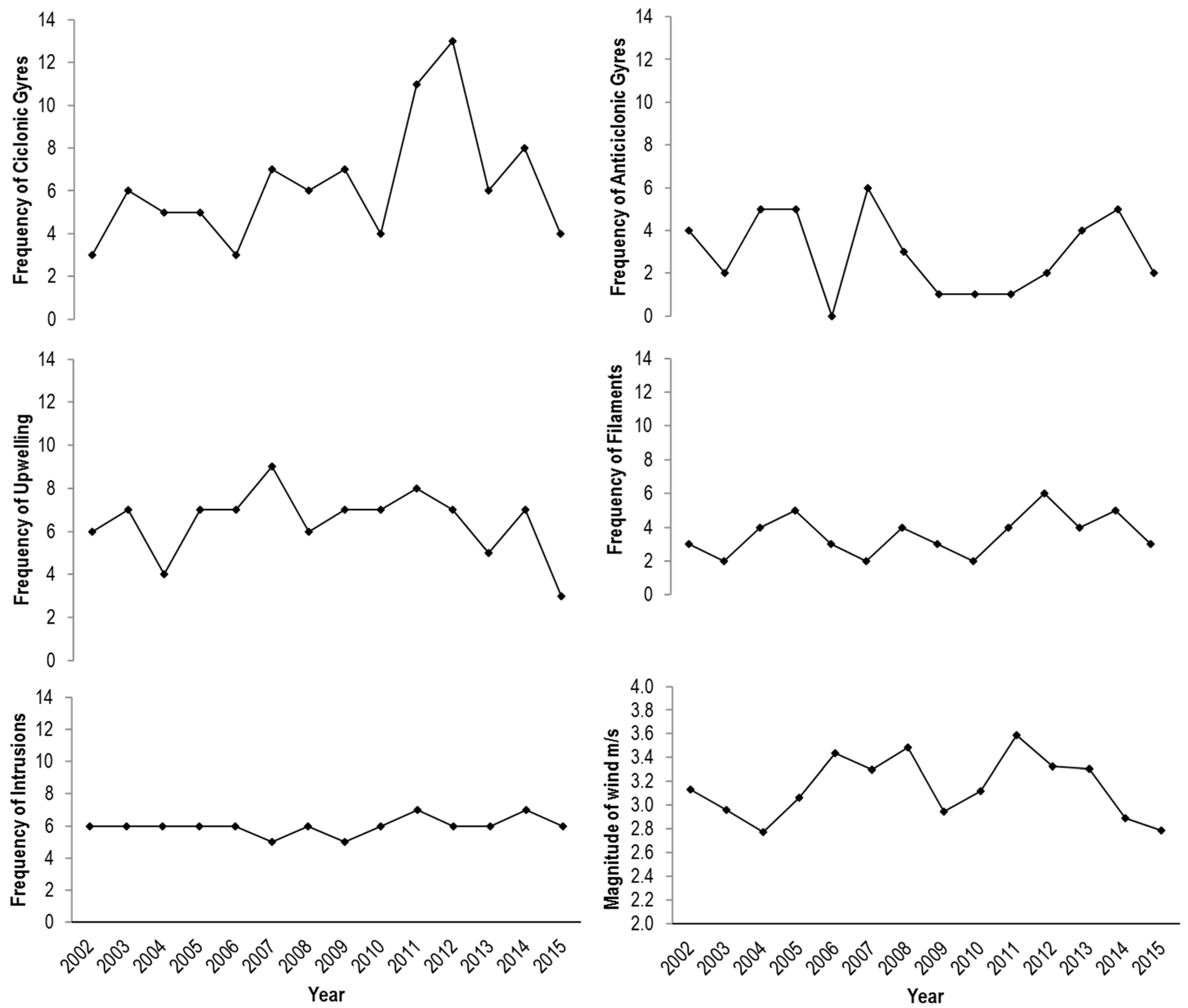
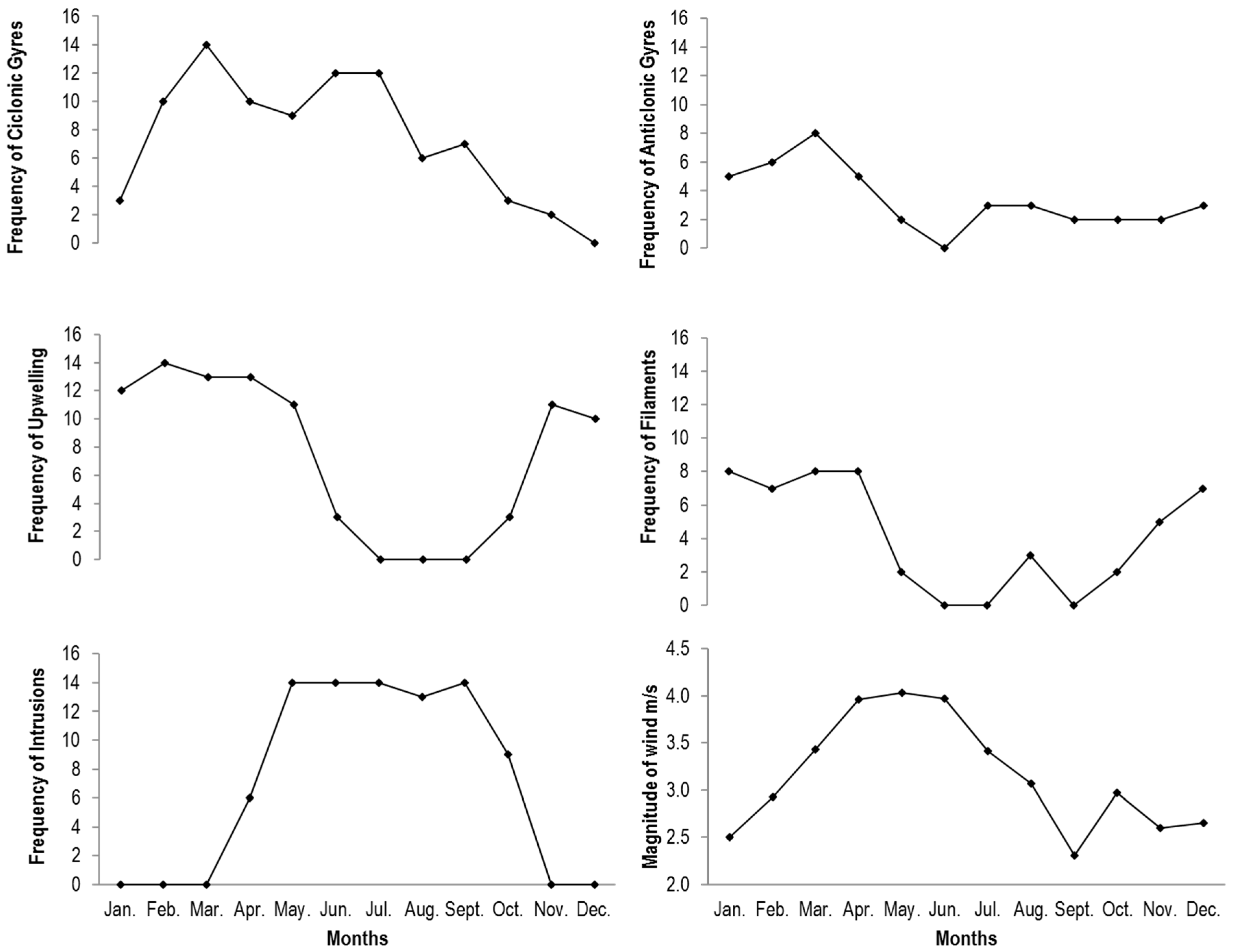
3.1. Analyses of Cumulative Annual and Monthly Frequency of Mesoscale Phenomena Observed in the Central and Southern Coastal Region of Sonora in the Gulf of California from 2002–2015

A total of 336 monthly images of SST and Chl-a were analyzed, for which a total of 353 mesoscale phenomena were observed in the coastal region of Sonora and the adjacent deep zone to the GC with a cumulative monthly average of 29 ± 1.2, highlighting the months of February, March, April, May, June and July with greater frequency of mesoscale structures (37, 43, 42, 38, 29 and 29, respectively). The most frequent phenomena were cyclonic gyres, upwelling, and water intrusion with values of occurrence of 88, 90 and 84, respectively, followed by filaments and anti-cyclonic gyres. The upwelling seasonal pattern was clearly defined and extended from November–May with peaks in the months from January–April from 3.3–5.11 mg/m³. On the other hand, cyclonic gyres showed two maximum peaks of occurrence from February–April and from June–July. Another very persistent phenomenon in the GC was MCC water intrusion, which showed its arrival to the gulf with major frequency starting from May and extended permanency up to September. The highest wind magnitudes occurred from March–July and a period of less intensity from October–February (Figure 2).

Major structure frequencies were observed interannually in 2005, 2007, 2011, 2012 and 2014 with values of 28, 29, 31, 34 and 32, respectively, and a notable decrease in 2002, 2003, 2006, 2010 and 2015, of which 2015 was the year that showed the least number of phenomena with an annual total of 18. Likewise, an increasing trend was observed in the frequency of cyclonic gyres, filaments and intrusions and a decreasing trend in upwelling. As for anti-cyclonic gyres and upwelling, no trend was observed throughout the period of study, as well as no observation of anti-cyclonic gyres in 2006 due to the difficulty of determining them by the low concentration of Chl-a and intensification of the intrusion. The highest wind magnitudes occurred in 2006–2008 and 2011–2013. Variability was observed, although none of these trends were significant (Figure 3).

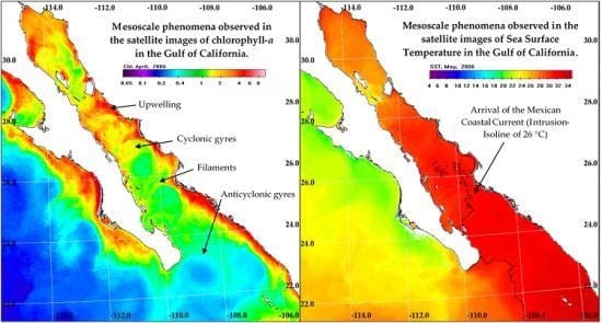
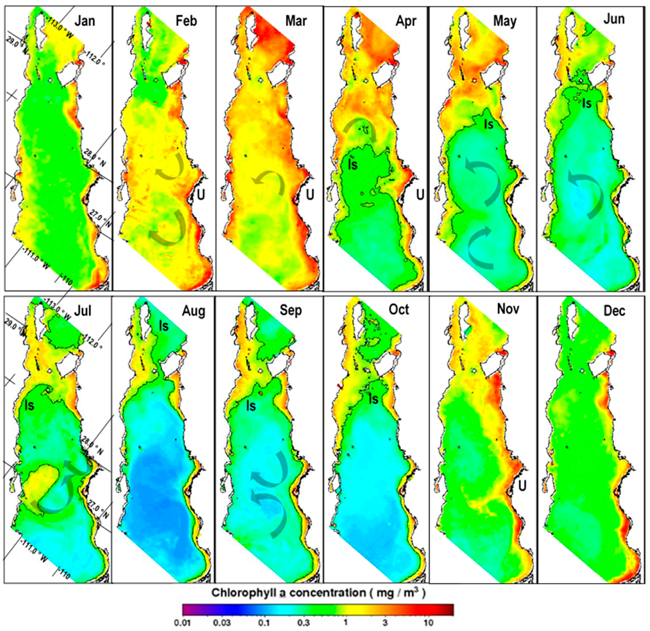
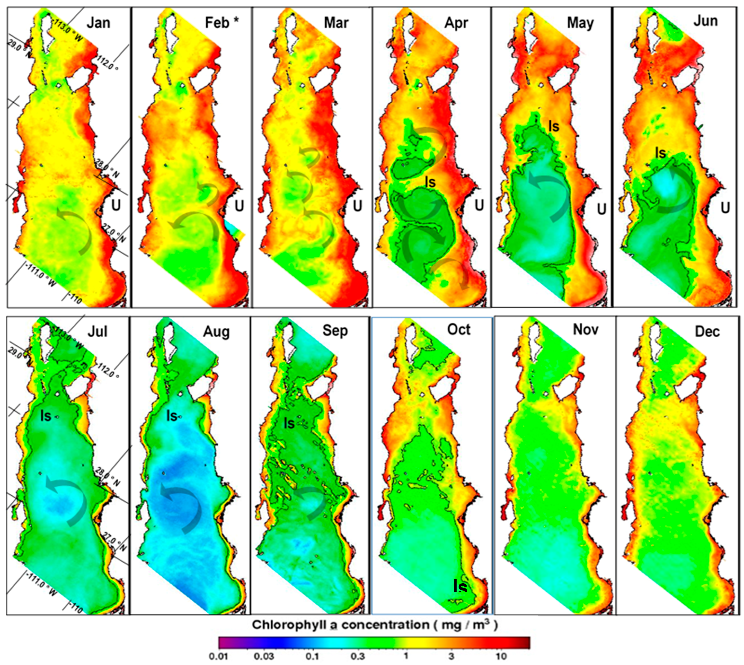
3.2. Analyses of Mesoscale Phenomena Observed Monthly by Images of Chlorophyll a

Monthly images of Chl-a were taken indistinctly in 2004 and 2012 to exemplify the analysis of the mesoscale phenomena; the years were chosen at random after determining that no significant differences were observed in the phenomena between years. Figure 4 shows the analysis for 2004 with a total frequency of 24 phenomena observed, mainly cyclonic and anti-cyclonic gyres from February–September and upwelling from February–April and in November. The presence of intrusion was observed from April–September, but more intensity was detected in August, reaching inclusively the northern GC area. Filaments were also observed with higher concentration of Chl-a extending toward the deep zone from April–November (Figure 4).

The year 2012 (Figure 5) was characterized by the greatest monthly frequency of the mesoscale phenomena observed with a total of 34. It was also characterized by showing a greater presence of cyclonic and anti-cyclonic gyres from January–September when March and April stood out with trains up to four gyres and intense upwelling in the area of study during the first half of the year. Water intrusion from the Pacific also took place from April–October 2012.

Figure 6 shows an example of warm water intrusion from the tropical Pacific through the MCC with SST greater than 26 °C by monthly SST images in May 2004 and 2012.

The results of analyzing the number of monthly observations and the length of the phenomena determined that the cyclonic gyres had a minimum length from one month up to a maximum of nine where 2003, 2009, 2011 and 2012 were the years when the greatest length of this phenomenon was observed with 5, 7, 5 and 9 months, respectively; 2011 and 2012 were those showing the greatest observation frequency of this phenomenon, recording an increasing trend the first 11 years with a sudden decrease the last three (2013–2015) (

Table 1. The number of monthly observations of phenomena per year, length in months of phenomenon per year, its mode of observation per month and its maximum length in the central and southern coastal region of Sonora and adjacent deep zone in the Gulf of California, Mexico, from 2002–2015.

Phenomena	Year
Cyclonic Gyres	2002			2003			2004			2005			2006			2007			2008			2009			2010			2011			2012			2013			2014			2015
No. of monthly observations of the phenomenon per year	3			6			5			5			3			7			6			7			4			11			13			6			8			4
Length of the phenomenon in months per year	1	1		1	5		1	3	1	2	1		1	1	1	2	2	3	2	1	2		7		1	3		6	3	1	9	2	2	2	2		2	4			4
Mode of phenomena observations per month	1			1			1			1			1			1			1			1			1			2			1			1			1			1
Maximum duration of the phenomenon in months	1			5			3			2			1			3			2			7			3			5			9			2			4			4
Anticyclonic Gyres
No. of monthly observations of the phenomenon/year	4			2			5			5						6			3			1			1			1			2			4			5			2
Length of the phenomenon in months per year	3	1		1	1		2	1	1	1	1	1				3	1	1	1	1	1		1			1			1			1		1	2		3	2		1	1
Mode of phenomena observations per month	1			1			1			1						1			1			1			1			1			1			1			1			1
Maximum duration of the phenomenon in months	3			1			1			1						3			1			1			1			1			1			2			3			1
Upwelling
No. of monthly observations of the phenomenon/year	6			7			4			7			7			9			6			7			7			8			7			5			7			3
Length of the phenomenon in months per year	5	1		5	2		3	1		4	3		5	2		6	3		2	2	2	5	2		5	2		6	2		6	1		4	1		5	2			3
Mode of phenomena observations per month	1			1			1			1			1			1			1			1			1			1			1			1			1			1
Maximum duration of the phenomenon in months	5			5			4			4			5			6			2			5			5			6			6			4			5			3
Filaments
No. of monthly observations of the phenomenon/year	3			2			4			5			3			2			4			3			2			4			6			4			5			3
Length of the phenomenon in months per year	1	1	1		2		1	1	2	2	1			3		1	1		1	1		2	1			2		3	1		4	1		1	2		2	1			3
Mode of phenomena observations per month	1			1			1			2			1			1			1			1			1			1			1			1			1			1
Maximum duration of the phenomenon in months	1			2			2			2			3			1			1			2			2			3			4			2			2			3
Intrusion
No. of monthly observations of the phenomenon/year	6			6			6			6			6			5			6			5			6			7			6			6			7			6
Length of the phenomenon in months per year		6			6			6			6			6			5			6			5			6			7			6			6			7		4	2
Mode of phenomena observations per month	1			1			1			1			1			1			1			1			1			1			1			1			1			1
Maximum duration of the phenomenon in months	6			6			6			6			6			5			6			5			6			7			6			6			7			5

Numerical values by columns and rows show the total number of phenomena observed by month and year, the length of the phenomenon by month (when there was more than one observation of the phenomenon per month, its length was considered for one month); thus, in some cases, the sum of lengths per month does not agree with the total observation of the phenomena per month.

and Figure 5). As for anti-cyclonic gyres, a minimum length of one month was established for the phenomenon in most of the years with a maximum of three months in 2002, 2007 and 2014 with an observation frequency of 4, 6 and 5, respectively, and a decreasing trend in the period of study. It is worth mentioning that no observation was recorded on this phenomenon in 2006.

In the analysis of monthly upwelling, a minimum length of one month and a maximum of six were observed with two upwelling periods, one five-month and two-month periods in 2002, 2003, 2006, 2009–2010 and 2014, although periods of up to six months were observed in this phenomenon in 2007 and 2011 with a decreasing trend. Filaments with high Chl-a were observed in the area of study with a minimum concentration of one month and a maximum of up to four in 2012, as well as a period of predominant observation of two months for this phenomenon in the majority of the years of study with an increasing trend. As for MCC water intrusion, a minimum of five months was observed in 2007, 2009 and 2015 and a maximum of seven in 2011 and 2014, where a six-month period predominated in the rest of the years, keeping stable during all of the period of study (Table 1).

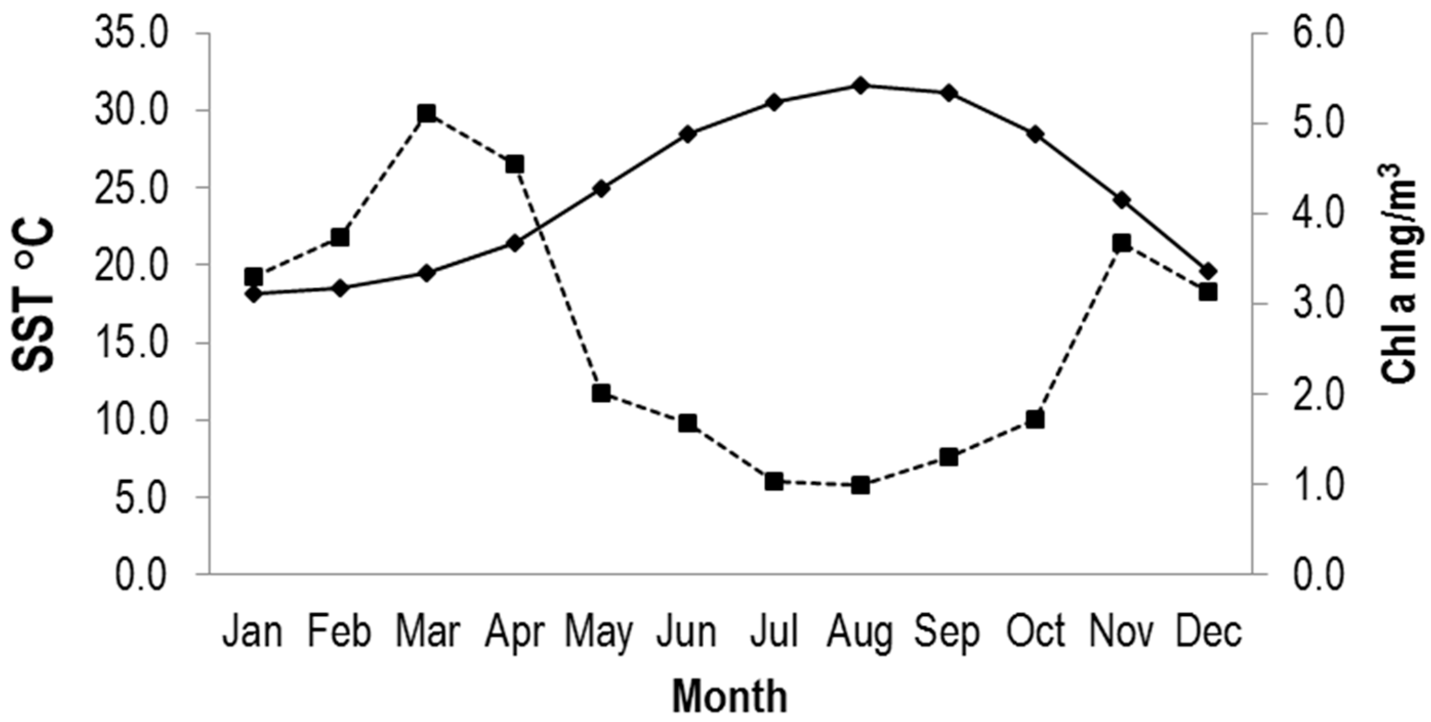
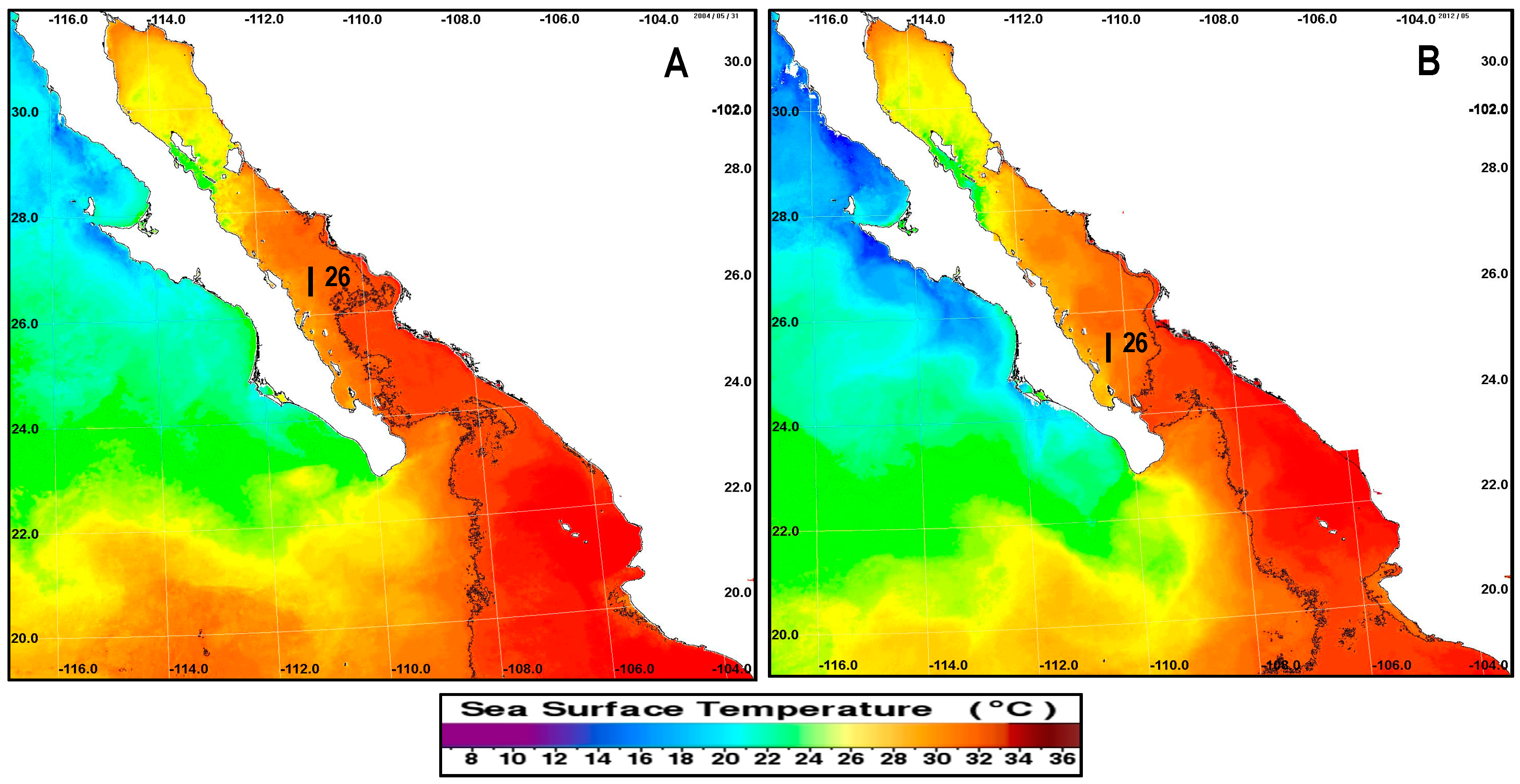
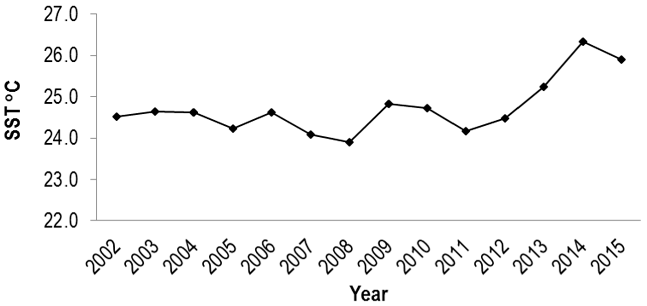
3.3. Monthly and Annual Analyses of Chlorophyll a, Sea Surface Temperature and Climate Indexes of the El Niño Southern Oscillation and Pacific Decadal Oscillation from 2002–2015

The average concentration of Chl-a showed a seasonal pattern with high values from 3.13–5.11 mg/m³ from November–April, reaching a maximum average of 5.11 ± 1.68 mg/m³ in March and low values with an average of 1.02 ± 0.25 mg/m³ from May–October, contrary to the SST, which showed average values ≥26 °C from June–October with a maximum average of 31.67 ± 0.51 °C in August and low values from 18 ± 1.29–24.9 ± 0.84 °C from November–April. It is worth mentioning that when SST values were ≥26 °C in May, they showed a decline of Chl-a; and when these values were ≤26 °C, they showed increased concentration of Chl-a in November (Figure 7).

An inverse lineal relationship (R² = 0.73) was observed between temperature and Chl-a concentration (Figure 8).

Higher concentrations of Chl-a were observed interannually from 2004–2012 with a temporal decrease in 2010. The highest one was recorded in 2009 with average values of 4.11 ± 3.58 mg/m³; the minimum value observed was 1.79 ± 1.03 mg/m³ in 2004 (Figure 9).

A minimum increasing trend in values of Chl-a was observed from 2002–2009, which started decreasing from 2013. As for average SST, fluctuations with values ranging from 23.89 ± 5.83–26.34 ± 4.39 °C were observed in 2008 and 2014, respectively, with a clear increasing trend (Figure 10).

In the annual analysis of environmental variables and the percentage of the mesoscale phenomena, no statistical differences (p > 0.05) were observed in the years assessed, indicating lesser variability in yearly values for the percentage of phenomena reported (

Table 2. Monthly and annual analysis of temperature, chlorophyll a and percentage of mesoscale phenomena observed in the central and southern coastal regions of Sonora and adjacent deep zone in the Gulf of California, Mexico, from 2002–2015.

	Environmental Variables		Percentage of Mesoscale Phenomena
	SST °C	Chl-a mg/m3	Cyclonic Gyres	Anti-Cyclonic Gyres	Upwelling	Filaments	Intrusions
Month
January	18.00 ± 1.29 bh	3.31 ± 2.22 ab	10.71 ± 16.17 ab	17.86 ± 18.13 a	42.86 ± 35.87 a	28.57 ± 21.08 a	0.00 ± 0.00 c
February	18.41 ± 1.83 bgh	3.74 ± 2.24 ab	27.03 ± 21.46 ab	16.22 ± 22.27 a	37.84 ± 19.66 a	18.92 ± 20.38 ab	0.00 ± 0.00 c
March	19.44 ± 1.46 bfgh	5.11 ± 1.68 a	32.56 ± 22.63 ab	18.60 ± 21.56 a	30.23 ± 28.18 ab	18.60 ± 18.29 ab	0.00 ± 0.00 c
April	21.36 ± 1.28 bdefgh	4.55 ± 1.53 a	23.81 ± 22.89 ab	11.90 ± 16.47 a	30.95 ± 16.77 ab	19.05 ± 23.18 ab	14.29 ± 21.15 bc
May	24.92 ± 0.84 bcdef	2.01 ± 1.07 bcf	23.68 ± 20.58 ab	5.26 ± 10.03 a	28.95 ± 20.26 ac	5.26 ± 7.26 ab	36.84 ± 20.08 ab
June	28.47 ± 0.65 ae	1.68 ± 1.68 cf	41.38 ± 23.36 a	0.00 ± 0.00 a	10.34 ± 12.67 bc	0.00 ± 0.00 b	48.28 ± 27.90 ab
July	30.61 ± 0.65 ac	1.02 ± 0.25 f	41.38 ± 23.99 a	10.34 ± 13.15 a	0.00 ± 0.00 c	0.00 ± 0.00 b	48.28 ± 28.21 ab
August	31.67 ± 0.51 a	1.02 ± 0.37 f	24.00 ± 18.54 ab	12.00 ± 0.00 a	0.00 ± 18.62 c	12.00 ± 31.09 ab	52.00 ± 0.27 ab
September	31.23 ± 0.39 a	1.31 ± 0.39 cf	30.43 ± 25.08 ab	8.70 ± 15.48 a	0.00 ± 0.00 c	0.00 ± 0.00 b	60.87 ± 27.09 a
October	28.50 ± 0.76 ad	1.70 ± 0.65 bcf	15.70 ± 27.66 ab	10.53 ± 10.72 a	15.79 ± 18.62 bc	10.53 ± 14.47 ab	47.37 ± 47.86 ab
November	24.27 ± 1.26 bcdefg	3.73 ± 1.37 ab	10.00 ± 14.01 ab	10.00 ± 10.03 a	55.00 ± 41.98 a	25.00 ± 20.69 ab	0.00 ± 0.00 c
December	19.92 ± 1.97 bfgh	3.00 ± 1.34 ac	00.00 ± 0.00 b	15.00 ± 16.98 a	50.00 ± 36.75 ab	35.00 ± 31.16 a	0.00 ± 0.00 c
Year
2002	24.52 ± 5.46 a	2.27 ± 1.62 a	13.64 ± 15.54 a	18.18 ± 17.53 a	27.27 ± 32.07 a	13.64 ± 17.21 a	27.27 ± 47.02 a
2003	24.65 ± 5.04 a	2.45 ± 1.90 a	26.09 ± 23.67 a	8.70 ± 10.76 a	30.43 ± 45.59 a	8.70 ± 15.05 a	26.09 ± 32.11 a
2004	24.61 ± 5.53 a	1.79 ± 1.03 a	20.83 ± 21.32 a	20.83 ± 22.29 a	16.67 ± 22.98 a	16.67 ± 33.43 a	25.00 ± 31.38 a
2005	24.24 ± 5.19 a	2.61 ± 2.02 a	17.86 ± 22.34 a	17.86 ± 22.95 a	25.00 ± 22.91 a	17.86 ± 24.31 a	21.43 ± 43.25 a
2006	24.62 ± 5.76 a	2.80 ± 1.99 a	15.79 ± 22.61 a	0.00 ± 0.00 a	36.84 ± 37.69a	15.79 ± 22.61 a	31.58 ± 43.30 a
2007	24.09 ± 5.22 a	2.75 ± 1.80 a	24.14 ± 21.65 a	20.69 ± 23.69 a	31.03 ± 28.45 a	6.90 ± 15.54 a	17.24 ± 22.98 a
2008	23.89 ± 5.83 a	3.17 ± 1.99 a	24.00 ± 23.81a	12.00 ± 16.57 a	24.00 ± 32.82 a	16.00 ± 14.97 a	24.00 ± 38.92 a
2009	24.83 ± 5.44 a	4.11 ± 3.58 a	30.43 ± 23.96 a	4.35 ± 7.22 a	30.43 ± 31.67 a	13.04 ± 19.82 a	21.74 ± 32.92 a
2010	24.71 ± 4.90 a	2.39 ± 1.34 a	20.00 ± 33.43 a	5.00 ± 9.62 a	35.00 ± 41.72 a	10.00 ± 16.60 a	30.00 ± 33.43 a
2011	24.16 ± 6.18 a	3.39 ± 1.78 a	35.48 ± 26.42 a	3.23 ± 4.81 a	25.81 ± 36.32 a	12.90 ± 16.76 a	22.58 ± 42.12 a
2012	24.48 ± 5.70 a	3.53 ± 1.94 a	38.24 ± 21.12 a	5.88 ± 8.25 a	20.59 ± 17.48 a	17.65 ± 18.45 a	17.65 ± 22.32 a
2013	25.23 ± 4.81 a	2.32 ± 1.71 a	24.00 ± 22.60 a	16.00 ± 18.28 a	20.00 ± 30.64 a	16.00 ± 17.53 a	24.00 ± 38.57 a
2014	26.34 ± 4.39 a	2.07 ± 1.05 a	25.00 ± 22.71 a	15.63 ± 18.23 a	21.88 ± 17.81 a	15.63 ± 18.23 a	21.88 ± 31.67 a
2015	25.90 ± 4.73 a	1.89 ± 1.08 a	22.22 ± 20.55 a	11.11 ± 11.49 a	16.67 ± 13.97 a	16.67 ± 13.97 a	33.33 ± 46.87 a

Median ± standard deviation. Different superindexes show statistical differences between months or years per environmental variable or mesoscale phenomenon (p < 0.05; i.e., a ≠ b ≠ c). Shaded values indicate the months that showed similar characteristics for each variable and mesoscale phenomenon. Numbers in bold represent the months that showed a greater difference than the other months in terms of their values and frequency of phenomena.

). Whereas the monthly analyses of the phenomena observed from 2002–2015 showed significant differences (p < 0.05) between months for temperature, chlorophyll, cyclonic gyres, upwelling and intrusions, no monthly statistical differences (p > 0.05) were observed in the anti-cyclonic gyres recorded by variability between months. For Chl-a, an increase in concentration was recorded from November–April with significantly higher concentrations in March (5.11 ± 1.68 mg/m³) and April (4.55 ± 1.53 mg/m³) (p < 0.05). Similar trends in upwelling and filaments were recorded with observations of significantly greater upwelling in November, January and February (55.00 ± 41.98, 42.86 ± 35.37 and 37.34 ± 19.66%, respectively) and for filaments in December and January (35.00 ± 31.16 and 28.57 ± 21.08%) (p < 0.05). For temperature and percentage of the intrusions observed, the increasing trend was recorded from June–September, showing August and September to be significantly hotter (31.67 ± 0.51 and 31.23 ± 0.39 °C, respectively, p < 0.05); for the intrusions observed, September showed a significantly greater percentage (60.37 ± 27.095; p < 0.05). According to the previous information, the increase in Chl-a concentration was related to similar increasing upwelling and filament trends in the same period; on the contrary lower concentrations agree with the periods where the percentages of upwelling and filaments decreased and with the temperature increase due to an increase of the MCC water intrusion percentage.

Table 3. Spearman’s (R²) correlation by month between temperature, chlorophyll a and mesoscale phenomena observed in the central and southern coastal regions of Sonora and adjacent deep zone in the Gulf of California, Mexico, from 2002–2015.

Correlation Per Month between Mesoscale Phenomena and Environmental Variables
	Environmental Variables		Mesoscale Phenomena					Effect
January	SST	Chl-a	Cyclonic Gyres	Anti-Cyclonic Gyres	Upwelling	Filaments	Intrusions	Upwelling ↑-Cyclonic and Anticyclonic Gyres ↓
Cyclonic Gyres					−0.56
Anti-cyclonic Gyres					−0.62
February								SST ↓-Chl-a ↑
SST		−0.78
March								SST ↓-Chl-a ↑
SST		−0.63
April								SST ↓-Chl-a ↑, Filaments ↑-Intrusions ↓
SST		−0.74
Filaments							−0.53
May								Cyclonic Gyres ↑-Upwelling ↓, Intrusion ↑-Filaments and Cyclonic Gyres ↓
Cyclonic Gyres					−0.67		−0.69
Filaments							−0.65
June								Intrusions ↑-Cyclonic Gyres and Upwelling ↓
Cyclonic Gyres							−0.67
Upwelling							−0.75
July								Cyclonic Gyres ↑-Chl-a ↑, Intrusions ↑-Cyclonic and Anticyclonic Gyres ↓
Chl-a			0.59
Cyclonic Gyres							−0.64
Anti-cyclonic Gyres							−0.69
August								Anticyclonic Gyres and Filaments ↑-Chl-a ↓, Intrusions ↑-Anticyclonic Gyres ↓
Chl-a				−0.60		−0.51
Anti-cyclonic Gyres							−0.54
September								Intrusions ↑-SST ↑, Intrusions ↑-Cyclonic Gyres ↓
SST							0.54
Cyclonic Gyres							−0.76
October								Intrusions ↑-SST ↑, Cyclonic and Anticyclonic Gyres ↑-SST ↓, Upwelling and filaments ↑-Chl-a ↑, Intrusions ↑-Chl-a ↓, Upwelling ↑-Filaments ↑
SST			−0.55	−0.54			0.54
Chl-a					0.69	0.60	−0.56
Upwelling						0.74
December								Upwelling ↑-Chl-a ↑, SST ↑-Upwelling ↓
SST					−0.58
Chl-a					0.65

The numerical values by the intersection of rows and columns show Spearman’s (R²) correlation between the environmental variables of the mesoscale phenomena and among them with significant statistical differences between the two variables (p < 0.05); the highest correlations are shown in bold. Arrows pointing upward (↑) mean increase and downward (↓) decrease.

shows the environmental variables and mesoscale phenomena with significant correlations (<0.05); the greatest correlations (R²) were inversely observed between temperature and Chl-a in February and April (−0.78 and −0.74, respectively); between upwelling and filaments directly in October (0.74); and upwelling and intrusions inversely in June (−0.75), while inversely between cyclonic gyres in September (−0.76). According to the previous information, when SST decreased from February–April, greater Chl-a concentrations were observed; when water intrusion was observed from May–September, a decrease was observed in Chl-a, cyclonic and anti-cyclonic gyres, upwelling and filaments, and an increase in SST from September–October. It could be observed that when upwelling and filaments increased and in turn when upwelling increased, filaments also increased.

In the monthly analyses of the environmental variables, winds and data of the ENSO and PDO climate indexes, no statistical differences were observed for ENSO and PDO (p > 0.05) among the months assessed; however, a period of negative anomalies for ENSO could be appreciated from January–April with values from −0.05 ± 0.44–−0.16 ± 0.71 and a period of positive anomalies from May–December with values from 0.01 ± 0.39–0.21 ± 0.96 with a negative anomaly of −0.21 ± 1.15 in August, which differs from the pattern previously observed. Whereas the annual analyses of climate indexes from 2002–2015 showed significant differences (p < 0.05) among the years analyzed, for ENSO and PDO, a five-year period of positive anomalies was observed from 2002–2006 with values from 0.16 ± 0.57–0.43 ± 0.26; it was followed by a restoration period of negative anomalies from 2007–2013 with values from −0.26 ± 0.10–−0.70 ± 0.34 except for 2009 when a positive anomaly was recorded, different from the pattern that had been observed. The years that showed greater anomalies were 2002 and 2009, both characterized as moderate Niños, and 2015, characterized as a very strong Niño; the years with greater negative anomalies were 2007–2008 and 2010–2011, characterized as moderate Niñas. In terms of wind intensity, a period of greater intensity was observed from March–June with values from 3.4–4 m/s (

Table 4. Monthly and annual analyses of temperature, chlorophyll a, winds and climate indexes of the El Niño Southern Oscillation and Pacific Decadal Oscillation in the central and southern coastal regions of Sonora and adjacent deep zone in the Gulf of California, Mexico, from 2002–2015.

	Environmental Variables			Climate Index
Month
	TSM °C	Chl-a mg/m3	Winds m/s	ENSO	PDO
January	18.00 ± 1.29 bh	3.31 ± 2.22 ab	2.40 ± 0.57 b	−0.12 ± 0.84 a	0.22 ± 1.17 a
February	18.41 ± 1.83 bgh	3.74 ± 2.24 ab	2.90 ± 0.79 bd	−0.16 ± 0.71 a	0.16 ± 1.08 a
March	19.44 ± 1.46 bfgh	5.11 ± 1.68 a	3.48 ± 0.59 ad	−0.11 ± 0.54 a	0.11 ± 1.07 a
April	21.36 ± 1.28 bdefgh	4.55 ± 1.53 a	4.00 ± 0.49 ac	−0.05 ± 0.44 a	0.17 ± 0.96 a
May	24.92 ± 0.84 bcdef	2.01 ± 1.07 bcf	4.04 ± 0.42 a	0.01 ± 0.39 a	0.23 ± 1.05 a
June	28.47 ± 0.65 ae	1.68 ± 1.68 cf	4.05 ± 0.44 a	0.07 ± 0.42 a	0.06 ± 0.87 a
July	30.61 ± 0.65 ac	1.02 ± 0.25 f	3.38 ± 0.40 ad	0.11 ± 0.51 a	−0.18 ± 1.15 a
August	31.67 ± 0.51 a	1.02 ± 0.37 f	0.65 ± 0.48 bcd	−0.21 ± 1.15 a	−0.14 ± 1.42 a
September	31.23 ± 0.39 a	1.31 ± 0.39 cf	2.34 ± 0.72 b	0.17 ± 0.80 a	−0.33 ± 1.21 a
October	28.50 ± 0.76 ad	1.70 ± 0.65 bcf	2.96 ± 0.51 bd	0.21 ± 0.96 a	−0.31 ± 1.08 a
November	24.27 ± 1.26 bcdefg	3.73 ± 1.37 ab	2.58 ± 0.59 bd	0.21 ± 1.02 a	−0.31 ± 1.14 a
December	19.92 ± 1.97 bfgh	3.00 ± 1.34 ac	2.60 ± 0.52 bd	0.14 ± 1.09 a	0.06 ± 1.18 a
Year
2002	24.52 ± 5.46 a	2.27 ± 1.62 a	3.13 ± 0.79 a	0.62 ± 0.52 ac	0.22 ± 0.86 ae
2003	24.65 ± 5.04 a	2.45 ± 1.90 a	2.96 ± 0.94 a	0.28 ± 0.31 acd	0.97 ± 0.59 a
2004	24.61 ± 5.53 a	1.79 ± 1.03 a	2.77 ± 0.67 a	0.43 ± 0.26 acd	0.35 ± 0.46 ad
2005	24.24 ± 5.19 a	2.61 ± 2.02 a	3.06 ± 0.86 a	0.14 ± 0.41 ae	0.38 ± 1.03 ad
2006	24.62 ± 5.76 a	2.80 ± 1.99 a	3.44 ± 0.59 a	0.16 ± 0.57 ae	0.19 ± 0.61 ae
2007	24.09 ± 5.22 a	2.75 ± 1.80 a	3.30 ± 0.62 a	−0.40 ± 0.62 bde	−0.20 ± 0.63 bcde
2008	23.89 ± 5.83 a	3.17 ± 1.99 a	3.49 ± 0.91 a	−0.68 ± 0.42 be	−1.29 ± 0.37 b
2009	24.83 ± 5.44 a	4.11 ± 3.58 a	2.95 ± 0.67 a	0.33 ± 0.70 ac	−0.61 ± 0.79 bde
2010	24.71 ± 4.90 a	2.39 ± 1.34 a	3.12 ± 0.77 a	−0.33 ± 1.03 bce	−0.31 ± 0.95 bcde
2011	24.16 ± 6.18 a	3.39 ± 1.78 a	3.59 ± 0.94 a	−0.70 ± 0.34 be	−1.23 ± 0.66 be
2012	24.48 ± 5.70 a	3.53 ± 1.94 a	3.33 ± 0.96 a	−0.12 ± 0.39 bce	−1.10 ± 0.58 be
2013	25.23 ± 4.81 a	2.32 ± 1.71 a	3.30 ± 0.76 a	−0.26 ± 0.10 bde	−0.52 ± 0.41bde
2014	26.34 ± 4.39 a	2.07 ± 1.05 a	2.89 ± 0.84 a	0.01 ± 0.40 bce	1.13 ± 0.65 ac
2015	25.90 ± 4.73 a	1.89 ± 1.08 a	2.79 ± 0.77 a	1.26 ± 0.70 a	1.63 ± 0.49 a

Median ± standard deviation. Different superindexes show statistical differences among months or years per environmental variables, winds and climate indexes of the El Niño Southern Oscillation and Pacific Decadal Oscillation (p < 0.05; i.e., a ≠ b ≠ c). Shaded values in monthly analyses indicate the months that showed warm characteristics for ENSO and PDO climate indexes. Numbers in bold represent the months that showed cold characteristics for climate indexes and the months that showed higher wind intensity.

).

The environmental variables, mesoscale phenomena, winds and climate indexes that showed significant correlations (p < 0.05) are shown in

Table 5. Spearman’s (R²) correlation by month among temperature, chlorophyll a, mesoscale phenomena, winds and climate indexes observed in the central and southern coastal region of Sonora and adjacent oceanic zone in the Gulf of California, Mexico, from 2002–2015.

	Environmental Variables			Climate Index		Effect
January	SST	Chl-a	Winds	ENSO	PDO
SST				0.63	0.54	PDO and ENSO ↑-SST ↑-Chl-a ↓, ENSO ↓-Winds ↑, PDO ↑-ENSO ↑
Chl-a				−0.63	−0.70
ENSO			−0.65		0.68
February	SST	Chl-a	Winds	ENSO	PDO
SST				0.62	0.62	PDO and ENSO ↑-SST ↑-Chl-a ↓, PDO ↓-Winds ↑ PDO ↑-ENSO ↑
Chl-a				−0.68	−0.67
ENSO					0.79
PDO			−0.53
March	SST	Chl-a	Winds	ENSO	PDO
SST				0.61	0.74	PDO and ENSO ↑-SST ↑, PDO ↓-Chl-a and Cyclonic Gyres ↑, ENSO ↓-Filaments ↑
Chl-a					−0.67
Cyclonic Gyres					−0.67
Filaments				−0.55
April	SST	Chl-a	Winds	ENSO	PDO
SST			−0.59			PDO and ENSO ↓-Winds ↑, SST ↑-Winds ↓, PDO ↑-ENSO ↑
ENSO			−0.63		0.597
PDO			−0.53
May	SST	Chl-a	Winds	ENSO	PDO
SST			−0.63			SST ↑-Winds ↓, ENSO ↓-Winds ↑, ENSO ↑-Chl-a ↓ PDO ↑-ENSO ↑
Chl-a				−0.71
ENSO			−0.57		0.53
Jun	SST	Chl-a	Winds	ENSO	PDO
Chl-a				−0.59	−0.64	PDO and ENSO ↑-Chl-a ↓, PDO ↓-Winds ↑
PDO			−0.56
July	SST	Chl-a	Winds	ENSO	PDO
Chl-a					−0.71	PDO ↑-Chl-a ↓
August	SST	Chl-a	Winds	ENSO	PDO
Chl-a				−0.62		ENSO ↑-Chl-a ↓, ENSO ↓-Anti-cyclonic Gyres ↑, ENSO ↓-Intrusions ↓
Anti-cyclonic Gyres				0.65
Intrusions				−0.53
September	SST	Chl-a	Winds	ENSO	PDO
ENSO			−0.55		0.60	PDO and ENSO ↑-Winds ↓, PDO ↑-ENSO ↑
PDO			−0.55
October	SST	Chl-a	Winds	ENSO	PDO
Chl-a					−0.66	PDO ↑-Chl-a ↓, ENSO ↑-Winds and Cyclonic Gyres ↓, PDO ↑-Intrusions ↑
Cyclonic Gyres				−0.63
Intrusions					0.58
ENSO			−0.53		0.77
November	SST	Chl-a	Winds	ENSO	PDO
ENSO					0.72	PDO ↓-ENSO ↑
December	SST	Chl-a	Winds	ENSO	PDO
SST				0.72	0.55	PDO ↑- ENSO ↓-SST ↓, PDO ↑-ENSO ↑
ENSO					0.73

The numerical values by intersection of rows and columns show Spearman’s (R²) correlation among the environmental variables of mesoscale phenomena and El Niño Southern Oscillation and Pacific Decadal Oscillation climate indexes and among them with significant statistical differences between the two variables (p < 0.05); the highest correlations are shown in bold. Arrows point upward (↑) mean increase and downward (↓) decrease.

. Significant correlations (R²) were observed inversely between ENSO, PDO, and Chl-a in January, February, May, June, July and October (−0.63, −0.70, −0.68, −0.67, −0.71, −0.59, −0.64, −0.71, −0.66, respectively), which indicates that when positive anomalies of PDO and negatives of ENSO are present, Chl-a concentrations decrease. Moreover, inverse correlations were observed between ENSO and winds in January, April, May, September, and October (−0.65, −0.53, −0.57, −0.55 and −0.53, respectively), which clearly showed that as the negative phase of ENSO increased, so did wind intensity. This same effect happened with the correlation of PDO and winds for the months of February, April, June and September (−0.53, −0.63, −0.56 and −0.55, respectively) when the positive phase of PDO decreased. In March, an inverse correlation was recorded between ENSO and filaments of −0.55 and between PDO and cyclonic gyres with an inverse correlation of −0.67, that is when negative ENSO anomalies decreased in the positive PDO phase, the frequency of these two mesoscale phenomena increased. On the other hand, when negative ENSO anomalies occurred by August, the frequency of anti-cyclonic gyres increased with a correlation of 0.65. The significantly positive correlations were recorded between PDO, ENSO and SST for January, February, March and December (0.63, 0.54, 0.62, 0.62, 0.61, 0.74, 0.72, 0.55 respectively), which indicated that temperature increased in the area of study in the months when positive PDO and negative ENSO anomalies were recorded. The positive PDO and ENSO correlations were recorded in January, February, April, May, September, November and December (0.68, 0.79, 0.59, 0.53, 0.60, 0.72 and 0.73, respectively). Thus, when PDO anomalies were positive, ENSO anomalies were negative.

The performed analysis showed an important annual component and minor variability associated with the semiannual cycle (4–6 months). Chl-a series also showed evidence of a higher variation period variation, related to interannual (three year) cycles, possibly generated by El Niño-La Niña events. However, those frequencies are not supported by the analysis, because the sampling does not expand 10-times the period of the event (Figure 11).

4. Discussion

It is common to find mesoscale structures in the GC that have lead it to stand out as one of the most productive water bodies of the Pacific [5,12,62] because of the great number of oceanographic phenomena that occur, which agrees with the monthly analyses of the phenomena observed. They can be generated by the coupling processes of macroscale atmospheric phenomena and regional mesoscale events, which seem to occur each year [14].

The monthly frequency analyses showed a total of 353 mesoscale phenomena in the central and southern coastal regions of Sonora during the period of study where the months that stood out with greater observations per month of cyclonic gyres, upwelling and MCC water intrusion were from February–July. All of these phenomena have been the result of atmospheric forcing interaction in the Pacific where seasonal winds (with flux toward the southeast in winter and toward the northwest in summer) induced a significant barotropic variability in kinetic energy associated with gyres and upwelling, as well as in energy associated with fluctuations of the current force as mentioned by Badan-Dangón [15], Stammer and Wunsch [6] and Lavín et al. [14].

The results have shown a seasonal pattern of intense upwelling from November–May with a maximum observed from January–April, similar to that reported by Maluf and Lluch-Cota [8,9], who mentioned a period extending from November–April. In this same period, filaments with high Chl-a were observed, which according to Navarro-Olache et al. [16] Lavín et al. [54] and Zamudio [2] were generated by wind forcing in winter transporting cold water with a high concentration of Chl-a. They also mentioned that this same wind forcing forms cyclonic gyres responsible for high dispersion of Chl-a, as could be observed from January–April in our results. Likewise, these gyres play a fundamental role in the transport of suspended material, contributing to nutrient transport between the sub- and superficial layers, affecting the vertical and horizontal distribution of phytoplankton [66]. According to the previous information, the distribution and abundance of phytoplankton depend on the type of gyre and its time length, where anti-cyclonic gyres cause sinking of nutricline originating a low in primary local production. On the other hand, cyclonic gyres displace nutricline, and when this displacement is strong enough, it generates enrichment in the water column as for primary production exporting organic material to the ecosystem [67,68,69,70].

Likewise, according to the results of the monthly analyses and correlation, this pattern of upwelling and filaments of high Chl-a concentration was influenced by that of moderate and strong winds from November–April, caused by the cold phase of ENSO. It is characterized by wind intensification during these months, as well as a cooling factor of the superficial water layer in the tropical Pacific affecting the area of study [39,40]. Nonetheless, in the results of this study, the wind pattern was not correlated directly with the mesoscale phenomena, but the variations of these indexes affected wind intensity generating the type of mesoscale structures, such as upwelling, anti-cyclonic and cyclonic gyres, that are in charge of concentrating and dispersing high Chl-a concentration, respectively.

In the following months, climate indexes were directly correlated; in March, an increase in cyclonic gyres showed a decrease in the positive anomalies of PDO and an increase of filaments when ENSO showed a decrease in its negative anomalies; in August, an increase in anti-cyclonic gyres was observed when ENSO showed a sudden change from positive to negative anomalies, which also caused a decrease in intrusions. Finally, in October, a decrease of winds and cyclonic gyres was observed when the positive anomalies of ENSO increased. In the same manner, when the positive anomalies of PDO decreased in this month, intrusions increased.

The results showed a clear difference between cold and warm periods and variations between the same months in the central and southern coastal region of Sonora in the GC. The image analysis of Chl-a showed a similar variability to that of Espinosa-Carreón and Valdez-Holguín [17,71] who found a marked variability of Chl-a in the GC; they reported a high concentration during the cold period and a low one in the warm period, which agree with those shown in this study, where it could be clearly observed that as SST increased over 26 °C in the warm period, Chl-a showed a decrease; and when SST decreased, Chl-a showed a recovery in the area of study. This monthly variability was due to gale winds and upwelling during the cold period, as well as to gentle winds and warm water intrusion with oligotrophic characteristic of the Pacific to the GC [54,65,72]. The variability in Chl-a concentration previously mentioned, caused by changes in wind intensity and CCM intrusion, was also modulated by changes in the ENSO and PDO phases where our results showed that when the positive PDO phase decreased, Chl-a concentration increased, and when the positive ENSO phase increased, such a concentration decreased.

The results of the SST analysis corroborated the presence of two extreme periods in the annual temperature cycle in the area of study previously reported by Soto-Mardones et al. [11] Lavin and Marinone [42] and Godínez-Sandoval [63]. They concluded that SST variability was due to changes in solar radiation incidence that changed evaporation rates and wind intensity, as well as to the strong influence of MCC water intrusion from the Pacific Ocean through the mouth of the GC by means of coastal Kelvin type waves that spread along the continental coastline of the gulf, which were the ones transmitting signals from the Pacific to the inner GC [13]. Additionally, such extreme periods of high temperatures that went from June–October were influenced by the positive ENSO phase and by the negative PDO phase. On the contrary the period of lower temperatures was modulated by the negative ENSO phase and the positive PDO phase from November–May.

On the contrary, one of the intriguing results in the statistical analyses was that no significant differences were observed among the years of study for the SST and Chl-a variables and mesoscale phenomena. Nonetheless, in the analysis of climate indexes of PDO and ENSO, significant statistical differences were observed when a five-year period of positive temperature anomalies was observed for both indexes; a period of negative anomalies of up to seven years was also observed for both indexes with extreme years, such as 2002 and 2009 with positive anomalies, which were characterized as moderate Niños; 2015 was characterized as a strong Niño followed by a restoration period named Niña from 2007–2008 and 2010–2011. As explained by Bernal et al. [73], they suggested that annual temperatures were modulated mainly by the influence of great scale phenomena in the Pacific, as ENSO and PDO.

Likewise, the mesoscale phenomena that occurred in the area of study and those at the mouth of the GC were modulated by the three time scales that occur in the Mexican Tropical Eastern Pacific: (1) seasonal current (California Current and Mexican Coastal Current); (2) gyres (3–5 months) at the mouth of the gulf; and (3) interannual anomalies as El Niño and La Niña. These two last ones apparently play a role in MCC intensification during El Niño, as well as an increase in the number of gyres generated [13,74,75,76], which affect oceanographic dynamics of the GC. Likewise, Chl-a concentrations were observed in our results where its gradual increase and a gradual decrease of SST could be appreciated during the negative PDO and ENSO anomalies (2003–2009) with a decrease in Chl-a and an increase in SST in 2004, 2010 and 2015 caused by extreme warm events characterized as Niños (ENSO-NOAA).

According to the previous information, the decrease of Chl-a indicates an oligotrophic area associated with a low presence of organisms integrating phytoplankton and zooplankton, thus causing changes in their distribution and abundance, such as species displacement toward more productive areas or habitats where planktonic food is more abundant [50,51,52,77]. This behavior of the organisms could be explained by rotation movements or mechanisms of cyclonic gyres, which transport nutrients vertically toward the eutrophic zone, fertilizing it, and the phytoplankton responds to this pulse causing a phytoplankton bloom according to Coria-Monter et al. [26].

Likewise, according to Maluf [8], the interaction of the water mass from the Pacific with that of the GC and its characteristic topography and important circulation processes allow the formation of oceanic fronts provoking a convergence of organisms in the frontal areas of this mass of water and in the phenomena provoked by the same intrusion. Moreover, gyres retain and transport organisms and enrichment processes as upwelling and filaments that favor the habitat of a great number of organisms [14,24,25,26].

Previously in other studies, Soto-Mardones et al. (1999) showed that on average, the sea surface temperature (SST) of the Gulf of California decreases from the mouth to the head and its variability increases by using fourteen years of infrared satellite images (1983–1996) to examine SST variability. The annual scale accounts for most of the variability of the SST, which oscillates in phase with small variations from north to south. Escalante et al. (2013) using satellite-derived data from 1997–2010, sea surface temperature, chlorophyll a and primary productivity variations showed that interannual signals of El Niño (EN) and La Niña (LN) were more evident at the entrance to the gulf.

Likewise coinciding with these two works and with a series of larger data, López-Martínez et al. (2001) showed that interannual variation is one of the dominant signals in the Gulf of California by making a spectral analysis of TSM from 1952–1993 with data from a tide-chart located in Guaymas, Sonora, in the central part of the gulf, which agrees with that obtained in this study.

All of the physical, biological and atmospheric processes mentioned previously take place at different temporal and spatial scales, as our results have shown in the number of monthly observations of phenomena per year, their length in months per year and maximum length. Likewise, climate indexes and winds exert an influence on the coastal pelagic ecosystem of Sonora, providing productive and biologically-rich habitats for a great diversity of commercially-important species. Moreover, these different types of mesoscale phenomena in the area of study and their length could exert a positive or negative effect on some species, such as the production of eggs and larvae and the growth and survival in the stages of the different species populations that inhabit the GC as mentioned by Hammann et al. [78], Daskalov [79] and Nevarez-Martinez [24,25,80].

5. Conclusions

During the period analyzed, a large number of mesoscale phenomena could be observed in the area of study by analyzing images of Chl-a and SST, which determined the seasonal and annual variations in these two variables, as well as the frequency among phenomena from 2002–2015.

The mesoscale structures that could be detected were anti-cyclonic gyres, filaments of Chl-a concentrations besides upwelling, cyclonic gyres and MCC water intrusion, which were those that stood out. Likewise, the frequency observed of each one of the phenomena and their length could be determined to establish their possible effect on the ecosystem.

The analyses of oceanographic dynamics performed for months and years in the coastal central and southern area of Sonora in the Gulf of California allowed determining, in great measure, the evolution of its mesoscale superficial dynamics, which permitted establishing the oceanographic framework affecting the coastal area.

As for the Chl-a concentration, a wider period with high concentrations could be identified compared to those traditionally proposed for this area due to the upwelling phenomena, the negative phase of ENSO and the positive phase of PDO that took place from January–May and from November–December with a maximum in winter and spring. The minimum values were recorded in summer because of the strong impact in the area of study due to the effects of MCC water intrusion; in previous months, highly favorable conditions prevailed for the primary sustenance of the trophic nets, and all of a sudden, these conditions strongly decreased by such an intrusion with a consequent increase in SST in the positive phase of ENSO and the negative phase of PDO.

It was also determined that in the annual analyses of environmental variables and the percentage of mesoscale phenomena recorded, no significant differences were observed between the years assessed. While the monthly analyses of the phenomena recorded from 2002–2015 showed significant differences between months, for temperature, Chl-a, cyclonic gyres, upwelling, filaments and intrusions, no statistical monthly differences were observed in anti-cyclonic gyres because of the variability between months. A high correlation was observed between some environmental variables and mesoscale phenomena.

All of the physical and biological processes mentioned in this work, as well as their length, have a bearing in the state of health of the pelagic ecosystem of the coastal zone of Sonora, and they exert a positive or negative effect on the requirements of some biologically- and commercially-important species. Therefore, because of their importance, this type of studies should be monitored periodically to have updated environmental information of the ecosystems and their possible implications on the organisms.

References

1. Salazar-Sparks, J. Chile y la Comunidad del Pacífico; Editorial Universitaria: Santiago, Chile, 1999; 253p, ISBN 956111528X, 9789561115286. [Google Scholar]
2. Zamudio, L.; Hogan, P.; Metzger, E.J. Summer generation of the Southern Gulf of California eddy train. J. Geophys. Res. 2008, 113. [Google Scholar] [CrossRef]
3. Lluch-Cota, S.E. Gulf of California. In Marine Ecosystems of the North Pacific; PICES Special Publication: Sidney, BC, Canada, 2004; Volume 1, pp. 1–7, 1280. [Google Scholar]
4. Lavin, M.F.; Beier, E.; Badan, A. Estructura hidrográfica y circulación del Golfo de California: Escalas estacional e interanual. In Contribuciones a la Oceanografía Física en México: Monografía; Lavín, F., Ed.; Unión Geofísica Mexicana: Ensenada, Baja California, México, 1997; pp. 141–171. [Google Scholar]
5. Álvarez-Molina, L.L.; Álvarez-Borrego, S.; Lara-Lara, J.R.; Marinone, S. Annual and semiannual variations of phytoplankton biomass and production in the central Gulf of California estimated from satellite data. Cienc. Mar. 2013, 39, 217–230. [Google Scholar] [CrossRef]
6. Stammer, D.; Wunsch, C. Temporal changes in eddy energy of the oceans. Deep Sea Res. 1999, 46, 77–108. [Google Scholar] [CrossRef]
7. Lluch-Cota, S.E.; Aragon-Noriega, E.A.; Arreguin-Sánchez, F.; Aurioles-Gamboa, D.; Bautista Romero, J.; Brusca, R.C.; Cervantes-Duarte, R.; Cortéz-Altamirano, R.; Del-Monte-Luna, P.; Esquivel-Herrera, A.; et al. The Gulf of California: Review of ecosystem status and sustainability challenges. Prog. Oceanogr. 2007, 73, 1–26. [Google Scholar] [CrossRef]
8. Maluf, L.Y. The Physical Oceanography. In Island Biogeography in the Sea of Cortez; Case, T.J., Cody, M.L., Eds.; University of California Press: Berkeley, CA, USA, 1983; pp. 26–45. [Google Scholar]
9. Lluch-Cota, S.E. Coastal upwelling in the eastern Gulf of California. Oceanol. Acta 2000, 23, 731–740. [Google Scholar] [CrossRef]
10. Ripa, P. Seasonal circulation in the Gulf of California. Ann. Geophys. 1990, 8, 559–564. [Google Scholar]
11. Soto-Mardones, L.; Marinone, S.G.; Parés-Sierra, A. Variabilidad espaciotemporal de la temperatura superficial del mar en el Golfo de California. Cienc. Mar. 1999, 25, 1–30. [Google Scholar] [CrossRef]
12. Marinone, S.G. A three-dimensional model of the mean and seasonal circulation of the Gulf of California. J. Geophys. Res. 2003, 108, 21–27. [Google Scholar] [CrossRef]
13. Herrera-Cervantes, H.; Lluch-Cota, D.B.; Gutiérrez-de-Velasco, G.; Lluch-Cota, S.E. The ENSO signature in sea-surface temperature in the Gulf of California. J. Mar. Res. 2007, 65, 589–605. [Google Scholar] [CrossRef]
14. Lavin, M.F.; Castro, R.; Beier, E.; Cabrera, C.; Godinez, V.M.; Amador-Buenrostro, A. Surface circulation in the Gulf of California in summer from surface drifters and satellite images (2004–2006). J. Geophys. Res. Oceans 2014, 119, 4278–4290. [Google Scholar] [CrossRef]
15. Badan-Dangon, A. Coastal circulation from the Galapagos to the Gulf of California. In The Sea, Pan Regional; Robinson, A.R., Brink, K.H., Eds.; John Wiley and Sons: Hoboken, NJ, USA, 1998; Volume 11, pp. 315–343. [Google Scholar]
16. Navarro-Olache, L.F.; Lavín, M.F.; Álvarez-Sánchez, L.G.; Zirino, A. Internal structure of SST features in the central Gulf of California. Deep Sea Res. II 2004, 51, 673–687. [Google Scholar] [CrossRef]
17. Espinosa-Carreón, L.; Valdez-Holguín, E. Variabilidad interanual de la clorofila en Golfo de California. Ecol. Appl. 2007, 6, 83–92. [Google Scholar] [CrossRef]
18. Hoffman, E.E.; Powell, T.M. Environmental variability effects on marine fisheries: Four case histories. Ecol. Appl. 1998, 8, 523–532. [Google Scholar]
19. López-Martínez, J.; Rodríguez-Romero, J.; Hernández-Saavedra, N.Y.; Herrera-Valdivia, E. Population parameters of the Pacific flagfin mojarra Eucinostomus currani (Perciformes: Gerreidae) captured by the shrimp trawling fishery in the Gulf of California. Rev. Biol. Trop. 2011, 59, 887–897. [Google Scholar] [CrossRef] [PubMed]
20. Rodríguez-Romero, J.; Barjau, E.; Galván, F.; Gutiérrez, F.; López, J. Estructura espacial y temporal de la comunidad de especies de peces arrecifales de la Isla San José, Golfo de California, México. Rev. Biol. Trop. 2012, 60, 2. [Google Scholar]
21. Contreras-Catala, F.; Sánchez-Velasco, L.; Lavín, M.F.; Godínez, V.M. Three-dimensional distribution of larval fish assemblages in an anticyclonic eddy in a semi-enclosed sea (Gulf of California). J. Plankton Res. 2012, 34, 548–562. [Google Scholar] [CrossRef]
22. García-Reyes, M.; Largier, J.L.; Sydeman, W.J. Synoptic-scale upwelling indices and predictions of phyto-and zooplankton populations. Prog. Oceanogr. 2014, 120, 177–188. [Google Scholar] [CrossRef]
23. Lluch-Cota, S.E.; Morales Zárate, M.V.; Lluch Cota, D.B. Variabilidad del Clima y Pesquerías del Noroeste de México. En: Variabilidad Ambiental y Pesquerías de México; López-Martínez, J., Ed.; Comisión Nacional de Acuacultura y Pesca: Mazatlán, Sinaloa, México, 2008; p. 216. [Google Scholar]
24. Sánchez-Velasco, L.; Lavín, M.F.; Jiménez-Rosenberg, S.P.A.; Godínez, V.M.; Santamaría del Angel, E.; Hernández-Becerril, D.U. Three-dimensional distribution of fish larvae in a cyclonic eddy in the Gulf of California during the summer. Deep Sea Res. I Oceanogr. Res. Pap. 2013, 75, 39–51. [Google Scholar] [CrossRef]
25. Sánchez-Velasco, L.; Lavín, M.F.; Jiménez-Rosenberg, S.P.A.; Godínez, V.M. Preferred larval fish habitat in a frontal zone of the northern Gulf of California during the early cyclonic phase of the seasonal circulation (June 2008). J. Mar. Syst. 2014, 129, 368–380. [Google Scholar] [CrossRef]
26. Coria-Monter, E.; Monreal-Gómez, M.A.; Salas de León, D.A.; Aldeco-Ramírez, J.; Merino-Ibarra, M. Differential distribution of diatoms and dinoflagellates in a cyclonic eddy confined in the Bay of La Paz, Gulf of California. J. Geophys. Res. 2014, 6258–6268. [Google Scholar] [CrossRef]
27. Schwing, F.B.; Murphree, T.; Green, P.M. The Northern Oscillation Index (NOI): A New Climate Index for the Northeast Pacific. Prog. Oceanogr. 2002, 53, 115–139. [Google Scholar] [CrossRef]
28. Parrish, R.H.; Schwing, F.B.; Mendelssohn, R. Mid-Latitude Wind Stress: The Energy Source for Climate Shifts in the North Pacific Ocean. Fish. Oceanogr. 2000, 9, 224–238. [Google Scholar] [CrossRef]
29. Wooster, W.S.; Hollowed, A.B. Decadal-Scale Variations in the Eastern Subarctic Pacific, Winter Ocean Conditions. Can. Spes. Publ. Fish. Aquat. Sci. 1995, 121, 81–85. [Google Scholar]
30. Bograd, S.J.; Chereskin, T.K.; Roemmich, D. Transport of Mass, Heat, Salt, and Nutrients in the Southern California Current System: Annual Cycle and Interannual Variability. J. Geophys. Res. 2001, 106, 9255–9275. [Google Scholar] [CrossRef]
31. Bernal, P.A.; Chelton, D.B. Variabilidad biológica de baja frecuencia y gran escala en la Corriente de California, 1949–1978 (Low Frequency and Large-Scale Biological Variability in the California Current, 1949–1978). In Reports of the Expert Consultation to Examine Changes in Abundance and Species Composition of Neritic Fish Resources, Proceedings of the A Preparatory Meeting for the FAO World Conference on Fisheries Management and Development, San José, Costa Rica, 18–29 April 1983; FAO Fisheries Report; Csirke, J., Sharp, G.D., Eds.; The Food and Agriculture Organization of the United Nations (FAO): Rome, Italy, 1984; Volume 1, p. 102. [Google Scholar]
32. Schwing, F.B.; Murphree, T.; deWitt, L.; Green, P.M. The Evolution of Oceanic and Atmospheric Anomalies in the Northeast Pacific during the El Nino and La Nina Events of 1995–2001. Progr. Oceanogr. 2002, 54, 459–491. [Google Scholar] [CrossRef]
33. Deser, C.; Alexander, M.A.; Timlin, M.S. Evidence for a Wind-Driven Intensification of the Kuroshio Current Extension from the 1970s to the 1980s. J. Clim. 1999, 12, 1697–1706. [Google Scholar] [CrossRef]
34. Barlow, M.; Nigam, S.; Berbery, E.H. ENSO, Pacific Decadal Variability, and US Summertime Precipitation, Drought, and Stream Flow. J. Clim. 2001, 14, 2105–2128. [Google Scholar] [CrossRef]
35. Chiew, F.H.; McMahon, T.A. Global ENSO-Streamflow Teleconnection, Streamflow Forecasting and Interannual Variability. Hydrol. Sci. J. 2002, 47, 505–522. [Google Scholar] [CrossRef]
36. Trenberth, K.E. The Definition of El Niño. Bull. Am. Meteorol. Soc. 1997, 78, 2771–2777. [Google Scholar] [CrossRef]
37. Mantua, N.J.; Hare, S.R.; Zhang, Y.; Wallace, J.M.; Francis, R.C. A Pacific Interdecadal Climate Oscillation with Impacts on Salmon Production. Bull. Am. Meteorol. Soc. 1997, 78, 1069–1079. [Google Scholar] [CrossRef]
38. Mantua, N.J.; Hare, S.R. The Pacific Decadal Oscillation. J. Oceanogr. 2002, 58, 35–44. [Google Scholar] [CrossRef]
39. Mantua, N.J. The Pacific Decadal Oscillation and Climate Forecasting for North America; Joint Institute for the Study of the Atmosphere and Oceans, University of Washington: Seattle, WA, USA, 1999. [Google Scholar]
40. Piechota, T.C.; Garbrecht, J.D.; Schneider, J.M. Climate Variability and Climate Change. In Climate Variations, Climate Change, and Water Resources Engineering; Garbrecht, J.D., Piechota, T.C., Eds.; ASCE: Reston, VA, USA, 2006; pp. 1–18. [Google Scholar]
41. Makarov, V.G.; Jiménez-Illescas, A.R. Barotropic Background Currents in the Gulf of California. Cienc. Mar. 2003, 29, 141–153. [Google Scholar] [CrossRef]
42. Lavín, M.F.; Palacios-Hernández, E.; Cabrera, C. Sea Surface Temperature Anomalies in the Gulf of California. Geofís. Int. 2003, 42, 363–375. [Google Scholar]
43. Latif, M.; Barnett, T.P. Interactions of the Tropical Oceans. J. Clim. 1995, 8, 952–964. [Google Scholar] [CrossRef]
44. Zhang, Y.; Wallace, J.M.; Battisti, D.S. ENSO-Like Interdecadal Variability: 1900–93. J. Clim. 1997, 10, 1004–1020. [Google Scholar] [CrossRef]
45. Hare, S.; Mantua, N. Empirical Evidence for North Pacific Regime Shifts in 1977 and 1989. Progr. Oceanogr. 2000, 47, 103–145. [Google Scholar] [CrossRef]
46. Martinez, E.; Antoine, D.; D’Ortenzio, F.; Gentili, B. Climate-Driven Basin-Scale Decadal Oscillations of Oceanic Phytoplankton. Science 2009, 326, 1253–1256. [Google Scholar] [CrossRef] [PubMed]
47. Di Lorenzo, E.; Schneider, N.; Cobb, K.M.; Chhak, K.; Franks, P.J.S.; Miller, A.J.; McWilliams, J.C.; Bograd, S.J.; Arango, H.; Curchister, E.; et al. North Pacific Gyre Oscillation Links Ocean Climate and Ecosystem Change. Geophys. Res. Lett. 2008, 35, L08607. [Google Scholar] [CrossRef]
48. Lluch-Cota, S.E.; Parés-Sierra, A.; Magaña-Rueda, V.O.; Arreguín Sánchez, F.; Bazzino, G.; Herrera-Cervantes, H.; Lluch Belda, D. Changing climate in the Gulf of California. Prog. Oceanogr. 2010, 87, 114–126. [Google Scholar] [CrossRef]
49. Walther, G.-R.; Post, E.; Convey, P.; Menzel, A.; Parmesan, C.; Beebee, T.J.; Fromentin, J.M.; Hoegh-Guldberg, O.; Bairlein, F. Ecological responses to recent climate change. Nature 2002, 416, 389–395. [Google Scholar] [CrossRef] [PubMed]
50. Helmuth, B.; Harley, C.D.G.; Halpin, P.M.; O’Donnell, M.; Hofmann, G.E.; Blanchette, C.A. Climate change and latitudinal patterns of intertidal thermal stress. Science 2002, 298, 1015–1017. [Google Scholar] [CrossRef] [PubMed]
51. Lluch-Cota, S.E.; Tripp-Valdez, M.; Lluch-Cota, D.B.; Lluch-Belda, D.; Verbesselt, J.; Herrera-Cervantes, H.; Bautista-Romero, J.J. Recent trends in sea surface temperature off Mexico. Atmosfera 2013, 26, 537–546. [Google Scholar] [CrossRef]
52. Edwards, M.; Richardson, A.J. Impact of climate change on marine pelagic phenology and trophic mismatch. Nature 2004, 430, 881–884. [Google Scholar] [CrossRef] [PubMed]
53. Páez-Osuna, F.; Sánchez-Cabeza, J.A.; Ruiz-Fernández, A.C.; Alonso-Rodríguez, A.C.R.; Cardoso-Mohedano, J.G.; Flores-Verdugo, F.J.; Carballo, J.L.; Cisneros-Mata, M.A.; Piñón-Gimate, A.; Álvarez-Borrego, S. Environmental status of the Gulf of California: A review of responses to climate change and climate variability. Earth Sci. Rev. 2016, 162, 253–268. [Google Scholar] [CrossRef]
54. Kahru, M.; Marinone, S.G.; Lluch-Cota, S.E.; Parés-Sierra, A.; Mitchell, G. Ocean color variability in the Gulf of California: Scales from the El Niño-La Niña cycle to tides. Deep Sea Res. II 2004, 51, 139–146. [Google Scholar] [CrossRef]
55. Lavín, M.F.; Beier, E.; Gómez-Valdés, J.; Godínez, V.M.; García, J. On the summer poleward coastal current off SW México. Geophys. Res. Lett. 2006, 33. [Google Scholar] [CrossRef]
56. Pegau, W.S.; Boss, E.; Martínez, A. Ocean color observations of eddies during the summer in the Gulf of California. Geophys. Res. Lett. 2002, 29, 6-1–6-3. [Google Scholar] [CrossRef]
57. Kahru, M.; Kudela, R.M.; Manzano-Sarabia, M.; Mitchell, B.G. Trends in the surface chlorophyll of the California Current: Merging data from multiple ocean color satellites. Deep Sea Res. 2012, 77–80, 89–98. [Google Scholar] [CrossRef]
58. Kahru, M. Windows Image Manager, WIM Software (Ver. 9.06) and User’s Manual. 2016, p. 125. Available online: http://www.wimsoft.com/ (accessed on 28 June 2017).
59. Climate Prediction Center Internet Team NOAA/National Weather Service. National Centers for Environmental, Prediction, Climate, Prediction, Center. Available online: http://www.esrl.noaa.gov/psd/data/climateindices/list/ (accessed on 28 June 2017).
60. López, J.M. Variabilidad Anual e Interanual de la Clorofila-(SeaWiFS) y el Viento Superficial (QuikSCAT) en el Alto Golfo de California: Su Circulación y Asociación. Master’s Thesis, Universidad Autónoma de Baja California, Ensenada, Mexico, 2005; p. 71. [Google Scholar]
61. García-Morales, R.; Shirasago-German, B.; Felix-Uraga, R.; Perez-Lezama, E.L. Conceptual Model of Pacific Sardine Distribution in the California Current. Curr. Dev. Oceanogr. 2012, 5, 27–47. [Google Scholar]
62. Lavín, M.F.; Marinone, S.G. An overview of the physical oceanography of the Gulf of California. In Nonlinear Processes in Geophysical Fluid Dynamics; Velasco Fuentes, O.U., Sheinbaum, J., Ochoa, J., Eds.; Kluwer Academic Publishers: Dordrecht, The Netherlands, 2003; pp. 173–204. [Google Scholar]
63. Godínez-Sandoval, V.M. Dinámica y Termodinámica en la Entrada Exterior al Golfo De California. Ph.D. Thesis, Facultad de Ciencias Marinas, UABC, México, 2011; p. 139. [Google Scholar]
64. Morel, A.; Berthon, J.F. Surface pigments, algal biomass profiles, and potential production of the euphotic layer: Relationships reinvestigated in view of remote-sensing applications. Limnol. Oceanogr. 1989, 34, 1545–1562. [Google Scholar] [CrossRef]
65. Santamaría del Ángel, E.; Álvarez-Borrego, S.; Muller-Karger, F. Gulf of California biogeographic regions based on coastal zone color scanner imagery. J. Geophys. Res. 1994, 99, 7411–7421. [Google Scholar] [CrossRef]
66. McGillicuddy, D.J., Jr.; Robinson, A.R.; Siegel, D.A.; Jannasch, H.W.; Johnsonk, R.; Dickey, T.D.; McNeil, J.; Michaels, A.F.; Knapk, A.H. Influence of mesoscale eddies on new production in the Sargasso Sea. Nature 1998, 394, 263–265. [Google Scholar] [CrossRef]
67. Duxbury, A.C.; Duxbury, A.B.; Sverdrup, K.A. An Introduction to the World’s Oceans, 6th ed.; McGraw-Hill: New York, NY, USA, 2000; 528p. [Google Scholar]
68. Morrow, R.; Fang, F.; Fieux, M.; Molcard, R. Anatomy of three warm-core Leeuwin current eddies. Deep Sea Res. II 2003, 50, 2229–2243. [Google Scholar] [CrossRef]
69. Van Aken, H.M.; Van Veldhoven, A.K.; Veth, C.; De Ruijter, W.P.M.; Van Leeuwen, P.J.; Drijfhout, S.S.; Whittle, C.P.; Rouault, M. Observations of a young Agulhas ring, Astrid, during MARE in March 2000. Deep Sea Res. II 2003, 50, 167–195. [Google Scholar] [CrossRef]
70. McGillicuddy, D.J., Jr.; Anderson, L.A.; Bates, N.R.; Bibby, T.; Buesseler, K.O.; Carlson, C.A.; Davis, C.S.; Ewart, C.; Falkowski, P.G.; Goldtwaith, S.A.; et al. Eddy/wind interactions stimulate extraordinary mid-ocean plankton blooms. Science 2007, 316, 1021–1026. [Google Scholar] [CrossRef] [PubMed]
71. Robinson, C.J.; Gómez-Gutiérrez, J.; de León, D.A.S. Jumbo squid (Dosidicus gigas) landings in the Gulf of California related to remotely sensed SST and concentrations of chlorophyll a (1998–2012). Fish. Res. 2013, 137, 97–103. [Google Scholar] [CrossRef]
72. Godínez, V.M.; Beier, E.; Lavín, M.F.; Kurczyn, J.A. Circulation at the entrance of the Gulf of California from satellite altimeter and hydrographic observations. J. Geophys. Res. 2010, 115, C04007. [Google Scholar] [CrossRef]
73. Bernal, G.; Ripa, P.; Herguera, J.C. Variabilidad oceanográfica y climática en el bajo Golfo de California: Influencias del trópico y Pacífico norte. Cienc. Mar. 2001, 27, 595–617. [Google Scholar] [CrossRef]
74. Palacios, D.M.; Bograd, S.J. A census of Tehuantepec and Papagayo eddies in the Northeastern Tropical Pacific. Geophys. Res. Lett. 2005, 32, L23606. [Google Scholar] [CrossRef]
75. Kessler, W.S. The circulation of the Eastern Tropical Pacific: A review. Prog. Oceanogr. 2006, 69, 181–217. [Google Scholar] [CrossRef]
76. Zamudio, L.; Hurlburt, H.E.; Metzger, E.J.; Tilburg, C.E. Tropical wave-induced oceanic eddies at Cabo Corrientes and the Maria Islands, Mexico. J. Geophys. Res. 2007, 112, C05048. [Google Scholar] [CrossRef]
77. Mills, C.E. JellyFish blooms: Are populations increasing globally in response to changing ocean conditions. Hydrobiologia 2001, 451, 55–68. [Google Scholar] [CrossRef]
78. Hammann, M.G.; Nevárez-Martínez, M.O.; Green-Ruíz, Y. Spawning habitat of the Pacific sardine (Sardinops sagax) in the Gulf of California: Egg and larval distribution 1956–1957 and 1971–1991. CalCOFI Rep. 1998, 39, 169–179. [Google Scholar]
79. Daskalov, G. Relating fish recruitment to stock biomass and physical environment in the Black Sea using generalized additive models. Fish. Res. 1999, 41, 1–23. [Google Scholar] [CrossRef]
80. Nevárez-Martínez, M.O. Producción de Huevos de la Sardina Monterrey (Sardinops Sagax Caeruleus) en el Golfo de California: Una Evaluación y Crítica. Master’s Thesis, CICESE, Ensenada, Mexico, 1990; p. 144. [Google Scholar]
Figure 1. Central and southern coastal zone of Sonora in the Gulf of California and regionalization (continuous line) for environmental and oceanographic analyses.
Remotesensing 09 00925 g001
Figure 2. Cumulative monthly frequency observed of mesoscale phenomena and winds in the central and southern coastal region and adjacent deep zone in the Gulf of California.
Remotesensing 09 00925 g002
Figure 3. Cumulative annual frequency observed of mesoscale phenomena and winds in the central and southern coastal region of Sonora and adjacent deep zone in the Gulf of California.
Remotesensing 09 00925 g003
Figure 4. Satellite images of chlorophyll a mg/m3 concentration in 2004. Isoline of Chl-a of 1 mg/m3 (Is) and upwelling (U). Arrows in the clockwise direction indicate anti-cyclonic gyres, and those in the counterclockwise direction indicate cyclonic gyres.
Remotesensing 09 00925 g004
Figure 5. Satellite images of chlorophyll a mg/m3 concentration in 2012. Isoline of Chl-a of one mg/m3 (Is) and upwelling (U). Arrows in the clockwise direction indicate anti-cyclonic gyres, and those in the counterclockwise direction indicate cyclonic gyres.
Remotesensing 09 00925 g005
Figure 6. Satellite images of sea surface temperature °C of May 2004 (A) and 2012 (B) of the Gulf of California and temperature isolines of 26 °C (I 26) arriving to the central and southern coastal region of Sonora and the adjacent deep zone in the Gulf of California.
Remotesensing 09 00925 g006
Figure 7. Variability of chlorophyll a (dotted line) and sea surface temperature (continuous line) in the central and southern coastal region of Sonora and adjacent deep zone in the Gulf of California.
Remotesensing 09 00925 g007
Figure 8. Relationship of sea surface temperature vs. chlorophyll a in the central and southern coastal region of Sonora and adjacent deep zone in the Gulf of California.
Remotesensing 09 00925 g008
Figure 9. Average annual variability of chlorophyll a in the central and southern coastal region of Sonora, Mexico, and adjacent oceanic zone in the Gulf of California.
Remotesensing 09 00925 g009
Figure 10. Average annual variability of sea surface temperature in the central and southern coastal region of Sonora, Mexico, and adjacent oceanic zone in the Gulf of California.
Remotesensing 09 00925 g010
Figure 11. Spectral analysis and periodograms for sea surface temperature (SST) (A,B) and the concentration of chlorophyll a (Chl-a) (C,D).
Remotesensing 09 00925 g011