An Improved Tomography Approach Based on Adaptive Smoothing and Ground Meteorological Observations


1
School of Geodesy and Geomatics, Wuhan University, 129 Luoyu Road, Wuhan 430079, China
2
Earth System Science Programme, Faculty of Science, The Chinese University of Hong Kong, Hong Kong, China
*
Author to whom correspondence should be addressed.
Remote Sens. 2017, 9(9), 886; https://doi.org/10.3390/rs9090886
Submission received: 10 June 2017
/
Revised: 20 July 2017
/
Accepted: 23 August 2017
/
Published: 25 August 2017
(This article belongs to the Special Issue Multi-Constellation Global Navigation Satellite Systems: Methods and Applications)
Abstract
:Using the Global Navigation Satellite System (GNSS) to sense three-dimensional water vapor (WV) has been intensively investigated. However, this technique still heavily relies on the a priori information. In this study, we propose an improved tomography approach based on adaptive Laplacian smoothing (ALS) and ground meteorological observations. By using the proposed approach, the troposphere tomography is less dependent on a priori information and the ALS constraints match better with the actual situation than the constant constraints. Tomography experiments in Hong Kong during a heavy rainy period and a rainless period show that the ALS method gets superior results compared with the constant Laplacian smoothing (CLS) method. By validation with radiosonde and European Centre for Medium-Range Weather Forecasts (ECMWF) data, we found that the introduction of ground meteorological observations into tomography can solve the perennial problem of resolving the wet refractivity in the lower troposphere and thus significantly improve the tomography results. However, bad data quality and incompatibility of the ground meteorological observations may introduce errors into tomography results.

1. Introduction
Water vapor (WV) is an important meteorological parameter and its distribution and dynamics are closely associated with weather phenomena, but it is also one of the most difficult meteorological parameters to characterize [1]. The Global Navigation Satellite System (GNSS) as a mean to monitor WV was first proposed by Bevis et al. in 1992 [2]. Since then, extensive research has been conducted [3,4,5]. In recent years, Li et al. have conducted a lot of studies about using multi-GNSS data to retrieve atmospheric parameters in real time [6,7,8].
In 2000, Flores et al. [9], Seko et al. [10] and Hirahara [11] first applied Global Positioning System (GPS) to troposphere tomography and all solved the 3D or 4D WV field in the least-squares scheme. Flores et al. proposed using horizontal smoothing, vertical smoothing and boundary conditions to solve the ill-posed problem and use the singular value decomposition to solve the inversion problem [9]. This method has been developed by many other scientists for troposphere tomography [12,13,14,15,16,17]. Other approaches to retrieve the 3D WV include algebraic reconstruction techniques [18,19] and estimating WV directly from raw GPS phase observations [20].
The main drawback of troposphere tomography is the difficulty in retrieving the vertical structure of the atmosphere when the GNSS network is flat in altitude [21]. In flat geometry, given one solution compatible with data, one can form another solution by simply interchanging two layers. Rohm and Bosy have demonstrated that the same tomography model could get better results in a mountainous area than in plain areas [14]. When the GNSS network covers a small area, the effective GNSS rays (rays passing from the top layer of the tomography model to the receivers) will concentrate around the zenith, which will increase the difficulty in retrieving the vertical structure of the troposphere. The GNSS network we used in Hong Kong is both flat and small, which will present more of a challenge.
In most tomography methods, constraints and a priori information are usually used to overcome the ill-posed problem and help retrieve the vertical structure of the troposphere. Investigations already performed show strong dependence on a priori reference data and constraints [12,15]. However, if a tomography method heavily relies on the a priori data, the tomography solutions will be very similar to the a priori data and the role of the GPS tomography technique will decrease. To drop the dependence on a priori information and retrieve a better vertical structure of the troposphere, this paper proposes a new tomography algorithm based on adaptive Laplacian smoothing (ALS) and Helmert variance component estimation (HVCE) (Section 3). We also introduce ground meteorological observations into tomography to constrain the wet refractivity (WR) in the lower troposphere. The tomography results are validated in the Hong Kong area during a heavy rain period and a rainless period with respect to radiosonde data and European Centre for Medium-Range Weather Forecasts (ECMWF) data (Section 4). Problems in introducing ground observations into tomography system are discussed in Section 5 and some conclusions are reached in Section 6.
2. The GNSS Network and Data Analysis
2.1. The Hong Kong SatRef Network
The Hong Kong SatRef network consists of 15 continuously operating reference stations equipped with the Leica Global Navigation Satellite System (GNSS) receivers and antennas (Figure 1). Each station is equipped with an automatic meteorological device to record temperature, pressure and relative humidity. With these data, the hydrostatic parts of the tropospheric delay can be accurately removed. These will be the advantages of the SatRef network for troposphere tomography. The mean horizontal distance between stations is about 10 km and the ellipsoidal heights of the 15 stations are within 350 m, making SatRef network a small flat network, which will bring more challenge in retrieving the vertical resolution of water vapor [21].
As shown in Figure 1, the Hong Kong area is divided into 4 × 5 grids in the horizontal domain with each grid having an East–West width of ~10 km and a North–South height of ~8 km. The troposphere over Hong Kong is divided into 13 layers from the ground to the top of the troposphere with each layer having a thickness of 800 m.
2.2. Data Analysis
To examine the performance and effectiveness of the tomography technique under different weather conditions, the experiment is conducted in two periods in 2015. One is from 20 July to 26 July when heavy rain attacked Hong Kong with the largest daily rainfall (~190 mm) in 2015 on 22 July. The other is from 1 August to 7 August when the weather is rainless. 14 days of GNSS observation data from the SatRef Network are processed by the precise point positioning (PPP) module in Bernese 5.0 software (Astronomical Institute of the University of Bern, Bern, Swiss) [22]. International GNSS Service (IGS) final orbit and clock products are used. The antenna phase center offsets and variations, phase wind-up, Earth tides, Earth rotation, ocean tides and relativistic effects are corrected by conventional methods detailed in [23]. Differential code biases are corrected by products from the Center for Orbit Determination in Europe. The ionospheric delay is eliminated at first order by forming the ionosphere-free combination of double frequencies. The higher-order terms are neglected. In Bernese 5.0, the tropospheric delay is modeled as in [22]:
where is the tropospheric path delay between station k and satellite i; is the observation time; , are the zenith and azimuth of satellite i as observed from station k; is the slant delay according to an a priori model; , is a (time-dependent) zenith path delay parameter and its mapping function; , are the (time-dependent) horizontal north and east troposphere gradient parameters.
In this data analysis, the Saastamoinen model [24] and Neill mapping functions (NMF) [25] are used to compute hydrostatic slant delay as a priori slant delay. So , and are tropospheric parameters to be estimated. Since the a priori zenith hydrostatic delay (ZHD) provided by the Saastamoinen model is not accurate and its inaccurate part will transfer to , the estimated is not accurate either, but their sum will be much more accurate. As pressure observations are available at each GNSS station, the ZHD can be accurately determined by the Saastamoinen model and we obtain zenith wet delay by removing accurate ZHD from the sum of a priori ZHD and . and are the total delay gradients. To obtain wet gradients, we remove the hydrostatic gradients by utilizing the meteorological data from surface observations and radiosonde [21,26,27]. Once the ZWD and wet gradients are obtained, the slant wet delays (SWD) can be retrieved by:
where are wet mapping functions from NMF; is the wet delay gradient in the north direction; is the wet delay gradient in the east direction; is the phase residuals to take into consideration the inhomogeneity.
3. Tomography Approach
3.1. General Methods and Existing Problems
Generally, to retrieve the 3D WV distribution, a discretization of the troposphere needs to be performed. The troposphere over this study area is divided into a finite number of voxels with each voxel having a constant WR. When a GNSS signal travels through the troposphere from its top to a GNSS receiver on the ground, it passes through several voxels and each voxel will produce a delay effect to the signal due to water vapor in it. The summation of the delays generated by all voxels equals to the SWD. So, we can obtain the basic equation for troposphere tomography by:
where is the SWD of the ith GNSS signal, is the WR of the jth voxel and is the intercept of the signal path in the jth voxel. Using all the suitable SWD observations at the same epoch, we can form the observation equation:
where is the vector of SWD, is the intercept matrix and is the vector of WR.
However, in a practical situation Equation (4) can be badly ill-posed and ill-conditioned due to the distribution of GNSS stations and the geometry of the satellites. The problem becomes worse when the GNSS network is flat [21]. To solve this problem, additional constraints or a priori information are usually used [9,16,17,21,28]. Three kinds of constraints are usually added:
Equations (5)–(7) are the vertical constraints, horizontal constraints and boundary conditions. When a priori information is used, Equation (8) is also needed.
As the horizontal variation of water vapor is reasonably small in a small region, the horizontal constraints can be easily established by imposing that the refractivity in a voxel is a weighted average of its neighbors in the same level [9,13,29]. As the water vapor varies rapidly in the vertical direction, some scientists tried to use external profiles as a priori information to constrain the distribution of water vapor [17,29,30] while some scientists still used the weighted average method to establish horizontal constraints [9,21]. The former method is more determined by a priori information than by the SWDs when the SWDs are not sufficient to retrieve the water vapor distribution. The latter can perform well in the horizontal direction but may perform badly in the vertical direction since a simple smoothing is not sufficient to describe the rapid change of water vapor in the vertical direction. Cao tried to use an exponential function to constrain the vertical distribution of water vapor, which is better than a simple weighted average but not as good as directly using a priori information [31]. The exponential function itself is determined by a priori information. The dependence on a priori information is one of the problems existing in tropospheric tomography. Another problem that needs to be emphasized is the regularization algorithm. Since additional constraints are imposed on the solutions artificially, we need to give the additional constraints appropriate weights to solve the ill-posed and ill-conditioned problem while keeping an acceptable accuracy. When the above two problems are solved, the tomography solution can be obtained:
where (i = 1, 2, 3, 4) are the weights of corresponding constraints.
3.2. Improved Tomography Algorithm
Before presenting the improved tomography algorithm, we will introduce the Laplacian smoothing and Helmert variance component estimation which are the basis of the new algorithm.
3.2.1. Laplacian Smoothing
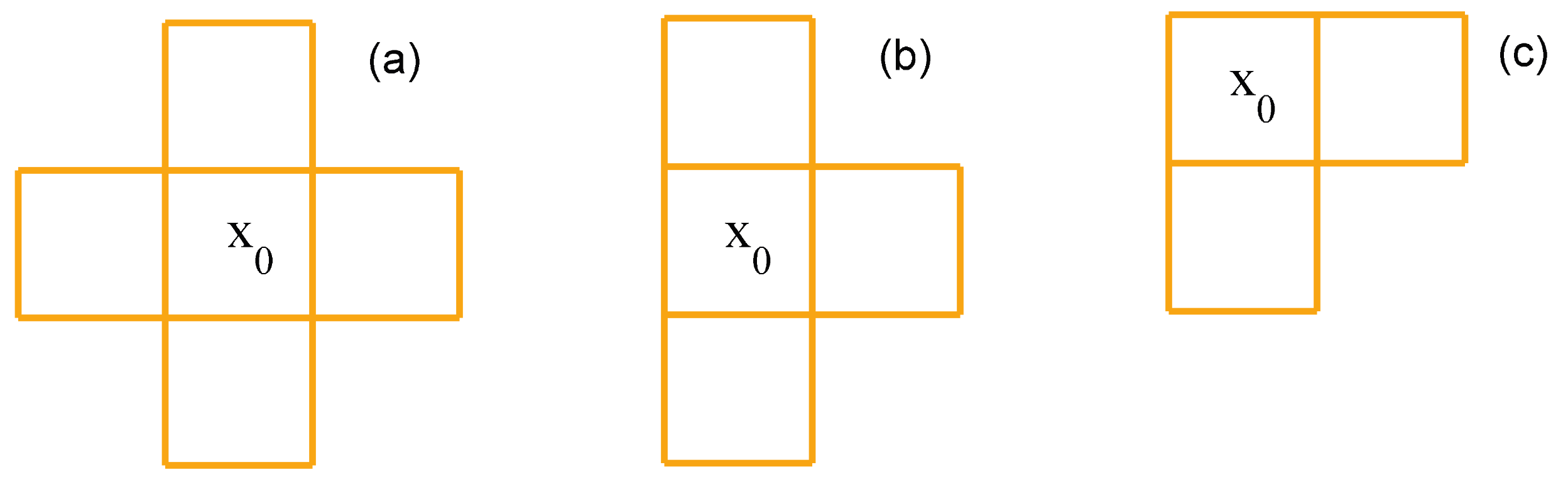
Laplacian smoothing is an algorithm to smooth a polygonal mesh based on the continuity of time or space. The smoothing operation is quite simple: the value of a voxel is replaced by the average of the values of its adjacent voxels. For the rectangular mesh in our case, we just consider the nearest four neighbors. Since our research area has strict boundaries, three situations will arise when we apply Laplacian smoothing, see Figure 2.
Assume that , , , are the wet refractivity in the nearest four voxels to and that the sizes of the voxels are the same, then according to Laplacian smoothing, we get:
for the situation in Figure 2a.
for the situation in Figure 2b.
for the situation in Figure 2c.
where is the smoothing factor whose initial values are 4, 3 and 2 for Equations (10)–(12), respectively. We use these three equations to construct constraints for each voxel in the horizontal and vertical directions, respectively. However, initial smoothing factors may be inaccurate, so we use an iterative feedback-update process to approach satisfactory results. Its basic idea is to use constraints to obtain results and then use results to update the constraints in turn. This process will be detailed later in Section 3.2.3.
3.2.2. Helmert Variance Component Estimation
After we construct the constraints, we use the Helmert variance component estimation [32,33] to determine the appropriate weights of the observations and constraints, and then estimate the tomography solution by Equation (9). According to Equations (4)–(8), we obtained five kinds of equations, so the equations for HVCE in this study can be written as:
where and are the variances of unit weight and residual vectors for five kinds of equations, respectively. Since the equations in Equations (4)–(8) are very few and not sufficient to determine all five weights, we chose to determine some weights before we ran HVCE. First, the wet refractivity in the top layer is constrained to zero and the boundary constraints are set to a very large weight (say 10,000). The weight of a priori information (if we have it) is set to be the same as the observations, namely 1. These three weights are considered unchangeable. Therefore, only and need to be determined by HVCE. Giving a small value to and as initial weights for vertical and horizontal constraints, can be estimated by Equations (9) and (13) in an iterative manner. During each iteration, the jth new weights are updated by:
The are repeatedly estimated until . After the iteration stops, we use the latest weights to estimate the solutions according to Equation (9).
3.2.3. The Adaptive Laplacian Smoothing Approach
In conventional tomography algorithms, observations and constraints unilaterally determine the results which have little effect on the constraints. However, the constraints are not always accurate, which will significantly affect the results. To establish the constraints as close to practical situations as possible, we build interaction between the constraints and results by developing an adaptive Laplacian smoothing algorithm. We first use the Laplacian smoothing to establish the initial vertical and horizontal constraints and use the HVCE method to estimate the initial solutions. We then use the initial solutions to estimate the smoothing factors q according to Equations (10)–(12) and establish the new horizontal and vertical constraints. We then resolve the new equations by HVCE. By an iterative feedback-update process, we could get better results than constant Laplacian smoothing (CLS). This new tomography algorithm can be performed by the following procedures:
(a) Use Equations (10)–(12) to construct the initial horizontal and vertical constraints respectively and initialize their weights as 1, namely . is set to a large value, is set to 1;
(b) Determine the values of and by HVCE and then calculate the tomography solutions by Equation (9);
(c) Update the smoothing factors by using the solutions from (b):
where n = 4 for Equation (10), 3 for Equation (11) and 2 for Equation (12). is a threshold set to prevent updating the smoothing factor by inaccurate solutions. The initial value for is half of the maximum wet refractivity in the solutions. is updated by multiplying by a scale factor, say 0.9, after each run until it is no larger than 3 times the mean square error of ;
(d) Use the new smoothing factors from (c) to update the horizontal and vertical constraints and redo (b) and (c) until the mean square error of the solution differences between this run and the previous run approaches a stable value. In practice, we set a threshold of 20 iterations which is enough to ensure a stable solution.
In conventional tomography methods, the constraints are constant and can’t be adjusted by solutions, namely initial constraints determine the final solution. In practice, the constraints are usually inaccurate and thus may bias the tomography results. In the new method, we establish a relationship between the constraints and solutions through an iterative feedback-update process. By this interactive adjustment, the constraints and solutions simultaneously approach the true values. The HVCE method helps to determine the weights for the constraints and observations. Appropriate constraints and weights make this a method better than the conventional ones.
3.3. Comparisons Between Adaptive Smoothing and Constant Smoothing
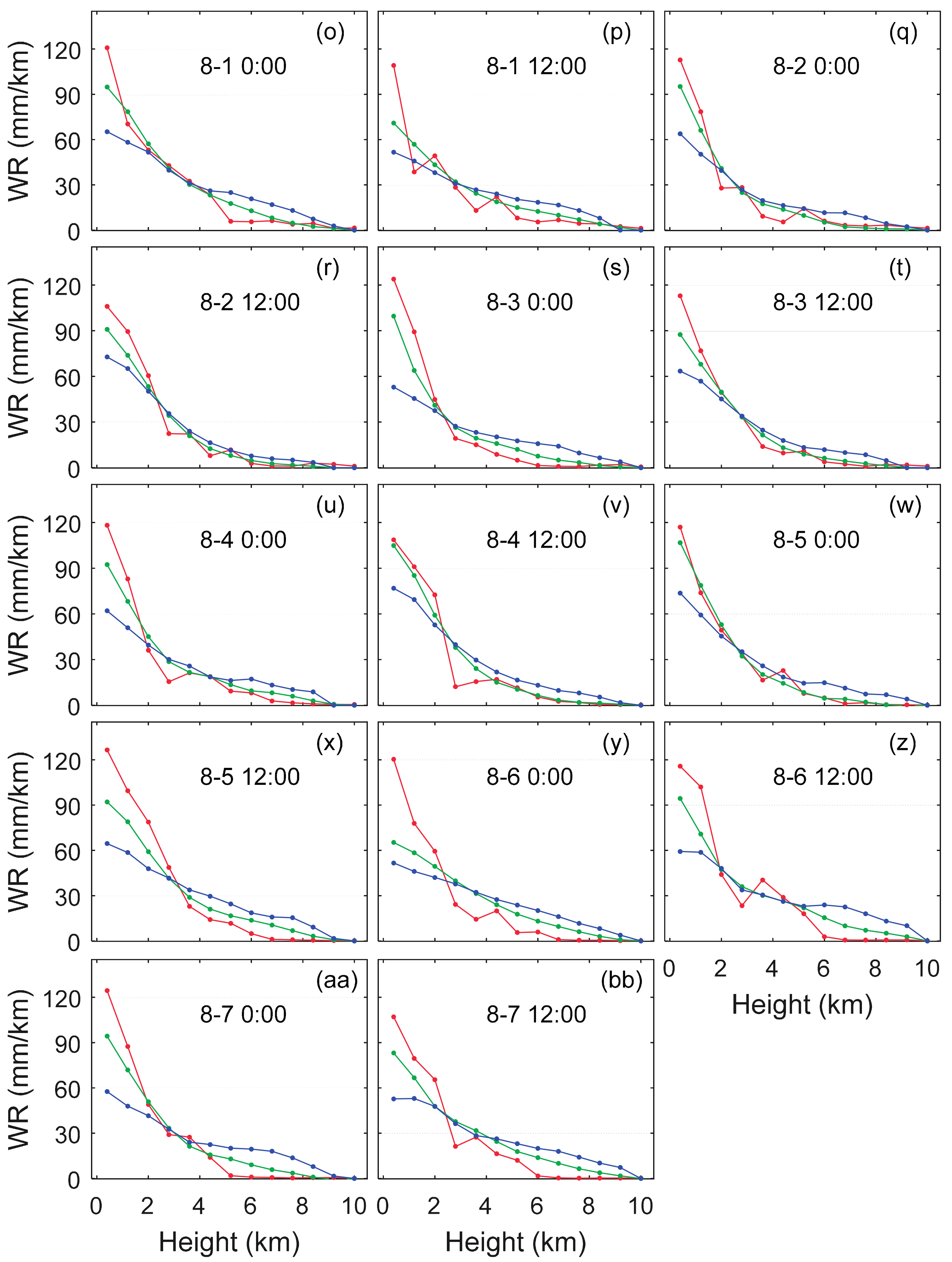
To verify the effectiveness of ALS, the tomography experiment is carried out with ALS and CLS, respectively, and no a priori information is used. Two periods of radiosonde data are used to validate the tomography results. One is from 20 July to 26 July when Hong Kong suffered heavy rain and the other is from 1 August to 7 August during rainless weather. Equation (16) is used to calculate wet refractivity for radiosonde data. Figure 3 shows the vertical WR obtained from radiosonde data, ALS and CLS constrained tomography results.
In Figure 3, almost all tomography results derived from the ALS method match better with the radiosonde WR profiles, indicating that the ALS method significantly improved the tomography results compared with the CLS method. However, the ALS method also obtained some results deviating from the radiosonde WR in the lower troposphere, though it was better than the CLS method. This is because most of the water vapor concentrates in the lower troposphere where it also changes more rapidly than above.
As is known, accurately determining the WR in the lower troposphere is still the most difficult part in troposphere tomography. To solve this problem, we introduced ground meteorological observations into the tomography system. In the Hong Kong SatRef network, radiosonde data and meteorological observations at each GNSS station are available. For radiosonde data, to reduce the dependencies on external data, only the observation nearest to the ground is used. The GNSS meteorological data include only surface temperature, humidity and pressure. We first used the Wexler formulations [34,35] to calculate vapor pressure from radiosonde and GNSS meteorological data and then calculated the WR according to Equation (16). We used the derived wet refractivity to establish a priori information equations according to Equation (8). When we solved the tomography equations, we found that the residuals of a priori information equations could be very large. Therefore, an extra procedure was performed to remove a priori information equations with residuals larger than 20 mm/km and then the tomography equations were resolved. This is an iterative process until no residuals are larger than 20 mm/km. Finally, about 50% of GNNS meteorological data are rejected.
4. Validation of the New Tomography Algorithm
In this section, radiosonde and ECMWF data are used to validate the tomography results. The validation was divided into two periods: one is from 20 July to 26 July when Hong Kong suffered heavy rain; the other is from 1 August to 7 August when the weather was rainless. Three strategies are used to conduct the tomography experiments. The first one is totally a priori information free (a priori information free strategy). The second one uses only the radiosonde observation closest to the ground to constrain the lower WR (one radiosonde observation constrained strategy). We don’t use the whole vertical radiosonde profile because we want to reduce the dependence on a priori information. The third one uses GNSS meteorological data to constrain the lower wet refractivity (GNSS meteorological data constrained strategy).
4.1. Comparison with Radiosonde Data
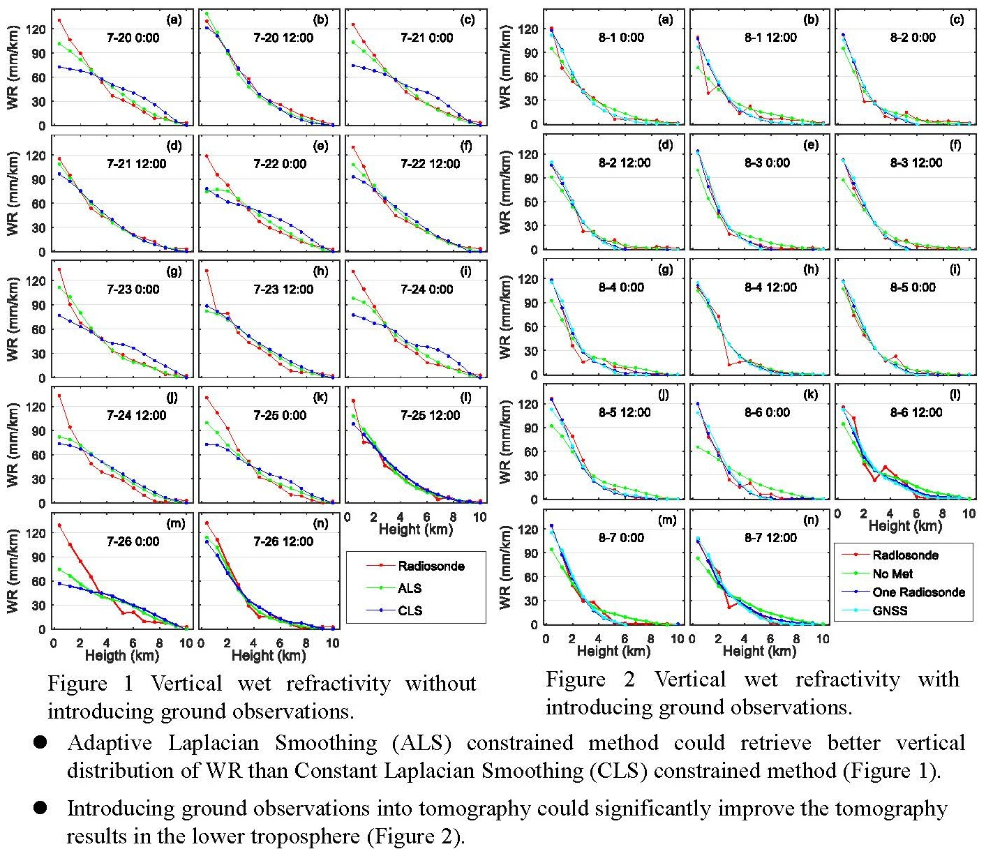
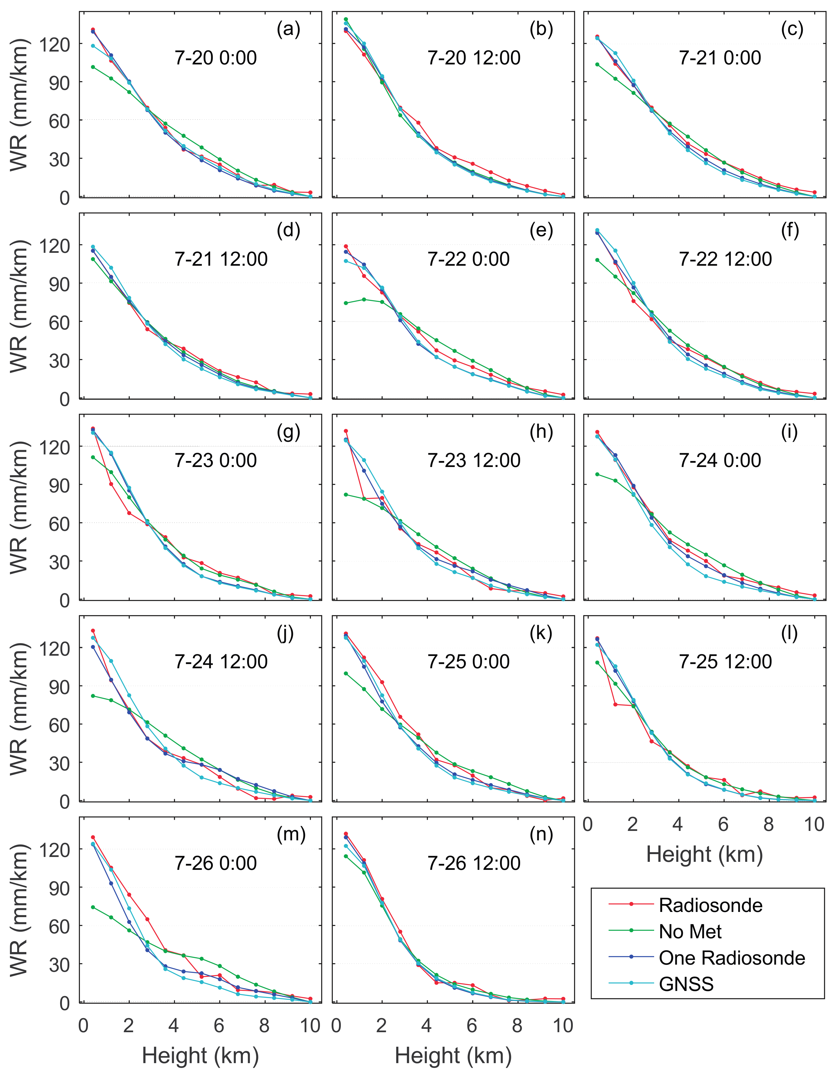
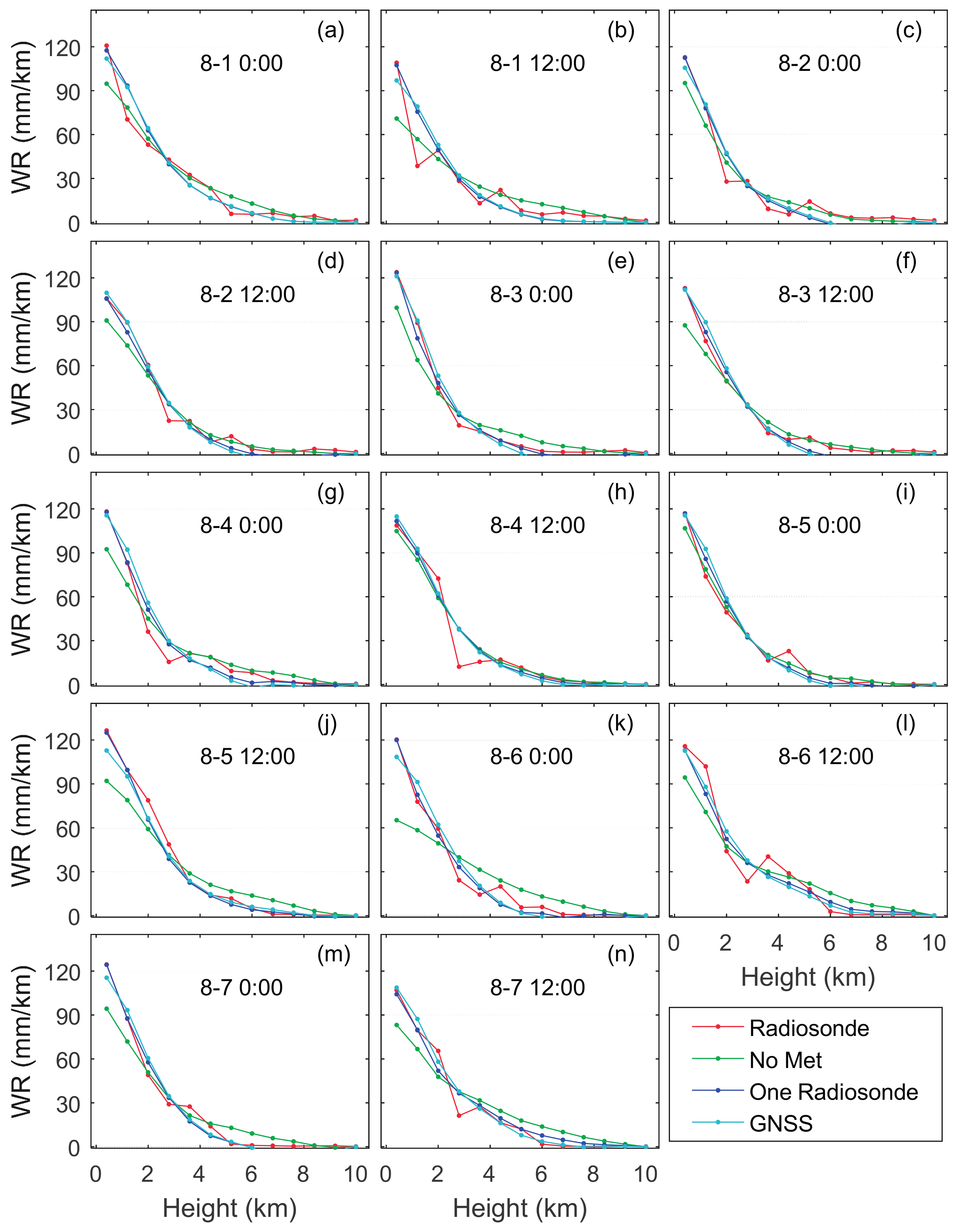
Since the radiosonde launches at 0:00, 12:00 UTC daily, we compare the radiosonde results with the tomography results at these time points. We first interpolate WR calculated from radiosonde data to the tomography voxel center. Figure 4 and Figure 5 show the comparisons between tomography and radiosonde results. It can be seen that all strategies can retrieve the vertical distribution of WR in most cases but the a priori information free strategy sometimes deviates from the radiosonde results in the lower troposphere. The one radiosonde observation constrained results and GNSS meteorological data constrained results are very similar, both matching better with the radiosonde results than the a priori information free results, especially in the lower troposphere. It can be seen that when only one radiosonde observation near the ground is used to constrain the results, the discrepancy between tomography results and radiosonde results can be sufficiently suppressed. This suggests that the constrained strategies make a compensation for the lower troposphere by introducing ground observations and make the tomography technique more capable of retrieving the vertical distribution of WR.
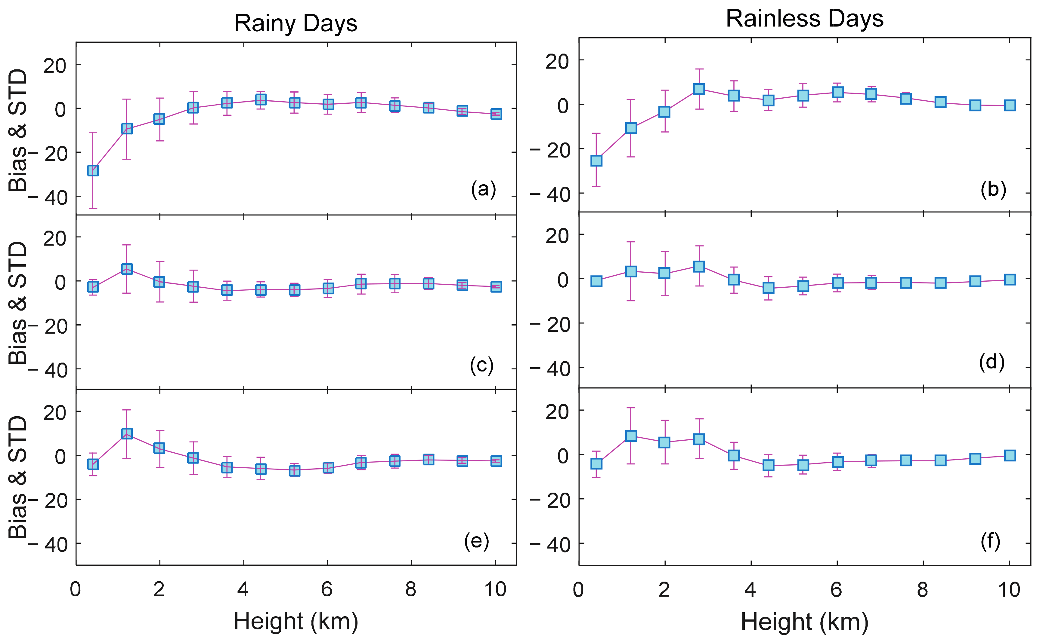
To gain knowledge of the vertical accuracy distribution, layered bias and standard deviation (STD) between the tomography and radiosonde results are calculated and shown in Figure 6. Comparing the subplots of different rows in Figure 6, we can see that the ground observation constrained strategies perform better than the a priori information free strategy by having a much smaller bias and STD. Both ground observation constrained strategies significantly improved the accuracy in the lower troposphere. In all subplots, the tomography results have a larger bias and STD below 3 km height than at greater heights, and the bias and STD decrease with increasing height. This can be explained by the fact that the water vapor is more concentrated and changeable in the lower troposphere than in the higher. In Figure 6a,b, the a priori information free strategy can obtain a good bias and STD at greater heights but it has a very large bias and STD in the lower troposphere. By introducing ground observations, this problem can be solved. Table 1 shows the statistics of the comparison between the tomography results and radiosonde results.
The statistics in Table 1 show that all strategies have lower accuracy in the low troposphere (height below 5.6 km) compared with the total mean accuracy, indicating again that it is difficult to accurately retrieve the WR in the lower troposphere. In both periods, the one radiosonde observation constrained strategy obtained the best accuracy, the GNSS meteorological data constrained strategy follows and the a priori information free strategy performs the worst. As for why the GNSS meteorological data constrained strategy is not as good as the one radiosonde constrained strategy, we think it should be due to local effects, height differences and observation errors. As the pressure, temperature and relative humidity measured by the GNSS meteorological equipment are close to the ground, the surroundings have a significant impact on the measurements. In addition, the tomography results are an average of WR within a voxel of size ~10 km × 10 km × 800 m. This makes the tomography results inconsistent with the ground observations, even though a height correction is already made and ground observations with large differences from tomography results are not used.
Comparing the results in the two periods, except in the case of the a priori information free strategy that has similar RMSE in both periods, ground observation constrained strategies have a relatively better accuracy in the rainy period than that in the rainless period with respect to STD or RMSE. In Figure 4 and Figure 5, the vertical distributions of wet refractivity are more even during the rainy days than those during rainless days. In Figure 5, the wet refractivity has large values below 5 km height and near 0 values above 5 km height, which indicates that the water vapor is more concentrated near the ground during this period than during rainy days. The evenly distributed water vapor is beneficial to obtain good tomography results from smoothing constrained methods, while the sharply changed distribution is not. This may explain why most STD and RMSE are smaller in the rainy period. However, the bias in the rainy period is much larger than that in the rainless period. Brenot et al. [36] and Kacmarik et al. [37] showed that the contribution of hydrometeors to GNSS signal delay can be as much as 20 mm or more, which is far from being negligible. In our data processing, the hydrometeors contribution is not removed thus may introduce a bias in the tomography results. There are more hydrometeors in the rainy period than in the rainless period, which may cause the bias of tomography results to be larger in rainy period than in the rainless period.
4.2. Comparison with ECMWF Data
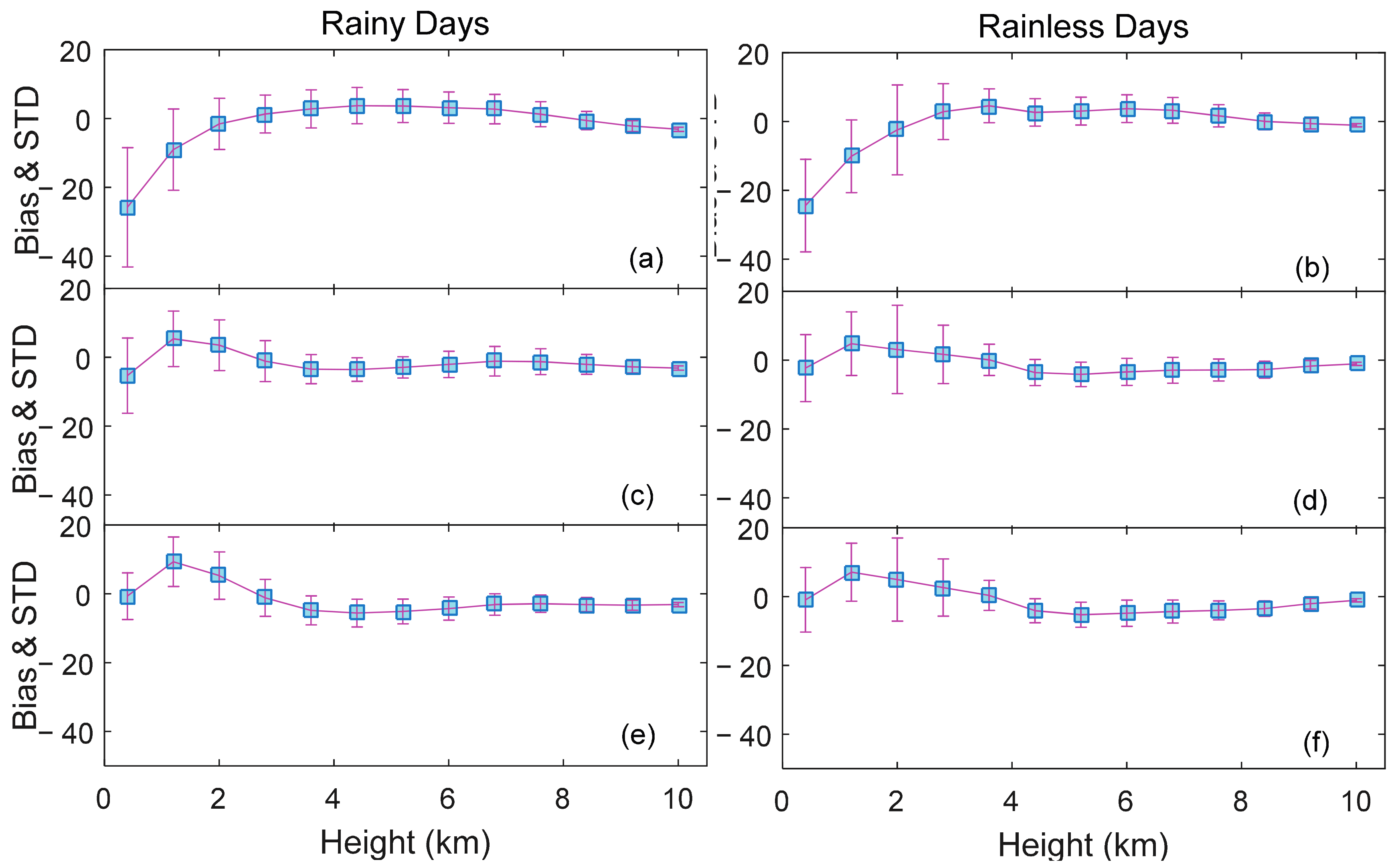
The comparison between tomography results and radiosonde data are limited to only one vertical column that the radiosonde station lies in, and the wet refractivity at the bottom is constrained by radiosonde observations, so this comparison may be not sufficient. Here we use ECMWF ERA-Interim data interpolated to a resolution of 0.125° to calculate and interpolate WR at the centers of the voxels. Then we calculate the bias, STD and RMSE between tomography results and ECMWF WR. Layered bias and STD are shown in Figure 7, and statistical data are shown in Table 2. Similar to the conclusions in Section 4.1, the ground observation constrained strategies obtained significantly better results than the a priori information free strategy. In this comparison, the GNSS meteorological data constrained strategy gets very similar results to the one radiosonde observation constrained strategy, both better than the a priori information free strategy with respect to STD or RMSE. Most of the bias in Table 2 is larger in the rainy period than in the rainless period, which is associated with hydrometeors in the atmosphere. The bias, STD and RMS derived from these three strategies decrease with increasing height and the results are better on the rainy days than the rainless days, which is consistent with the results in Section 4.1. The differences between the results in Table 1 and Table 2 should be due to the discrepancy which existed between the radiosonde data and ECMWF data.
5. Discussion
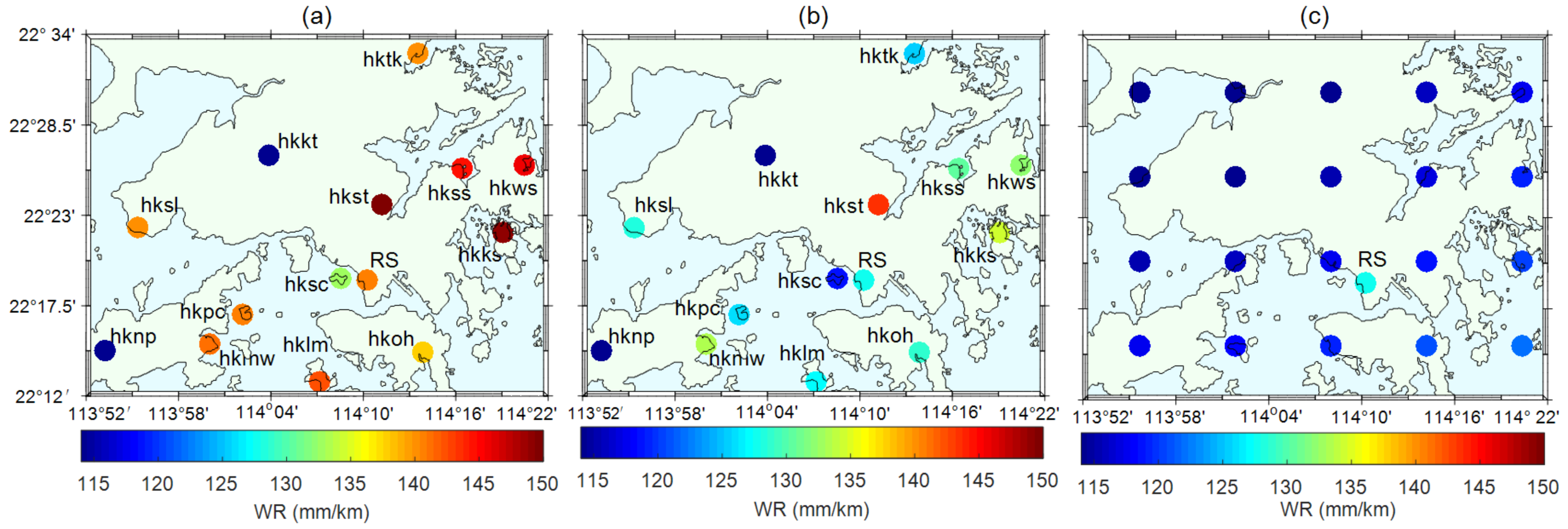
In our tomography experiments, observations were not sufficient in the lower troposphere, so introducing ground observations into the tomography system will be very helpful. However, the GNSS meteorological data constrained strategy led to a lower accuracy than the one radiosonde observation constrained strategy in both Section 4.1 and Section 4.2. To further investigate this problem, we used GNSS meteorological data, radiosonde data and ECMWF data to derive wet refractivity. Figure 8 shows an example which can represent most of the cases. Figure 8a shows the original GNSS meteorological data derived WR, Figure 8b shows a similar WR but reduced to 400 m height and Figure 8c shows the ECMWF derived WR at 400 m height. In Figure 8a, the WR from GNSS meteorological data shows sharp variations on the ground, but no clear gradient pattern can be observed. WR at site HKSC, which is closest to the RS site, is significantly different from the RS WR. This may be due to local effects, height differences and observation errors. In Figure 8b when GNSS meteorological data derived WR and RS WR are reduced to the same height of 400 m, the GNSS meteorological data derived WR still has sharp variations in the horizontal domain and a large difference still exists between HKSC and RS sites. This rules out the possibility of height differences causing WR variations. Figure 8c shows the ECMWF WR and RS WR, both reduced to 400 m height. In Figure 8c, ECMWF WR shows a clear gradient pattern that WR is decreasing from southeast to northwest. The ECMWF WR also has an obvious difference from RS WR. Assume that the gradient shown in Figure 8c is true, the fact that the gradient doesn’t show in Figure 8b should be mainly due to local effects since observation errors shouldn’t change the gradient pattern as much. The significant differences between RS WR and GNSS meteorological data derived WR (at HKSC) should be due to observation errors. WR at HKST is also very likely to have large errors since it is significantly larger than WR at other sites. Since the GNSS meteorological data derived WR is not as reliable as RS WR, we deleted GNSS meteorological data derived WR that were significantly incompatible with the tomography results when we performed tomography in an iterative way. By this additional procedure, we obtained the tomography results in Section 4.
6. Conclusions
We presented an improved tomography approach based on adaptive Laplacian smoothing and ground meteorological observations to reconstruct a three-dimensional wet refractivity field in Hong Kong under rainy and rainless weather conditions. By comparing tomography results with radiosonde and ECMWF data, we concluded that (1) adaptive Laplacian smoothing could retrieve better vertical distribution of WR than constant Laplacian smoothing, especially when no ground meteorological data is available (see Figure 3); (2) using ground observations to constrain the WR in the lower troposphere could significantly improve the tomography results in small flat networks (at least 29% of RMSE is reduced when compared with radiosonde data), but one should be cautious of the quality and compatibility of ground observations and (3) the tomography technique is affected by the vertical distribution of WR in small flat networks.
Acknowledgments
The authors would like to thank the Survey and Mapping Office/Lands Department of Hong Kong, IGRA and ECMWF for providing experimental data, and thank ECWMF for providing meteorological data. This research is supported by the National Natural Science Foundation of China (41704004).
Author Contributions
B.Z. and Q.F. conceived and designed the experiments and performed the experiments; Y.Y. and C.X. analyzed the data; B.Z. wrote the paper; X.L. revised the paper. All authors read and approved the submitted draft of the manuscript.
Conflicts of Interest
The authors declare no conflict of interest.
References
- Rocken, C.; Ware, R.; Van Hove, T.; Solheim, F.; Alber, C.; Johnson, J. Sensing atmospheric water vapor with the global positioning system. Geophys. Res. Lett. 1993, 20, 2631–2634. [Google Scholar] [CrossRef]
- Bevis, M.; Businger, S.; Herring, T.A.; Rocken, C.; Anthes, R.A.; Ware, R.H. GPS meteorology: Remote sensing of atmospheric water vapor using the Global Positioning System. J. Geophys. Res. Atmos. 1992, 97, 15787–15801. [Google Scholar] [CrossRef]
- Duan, J.; Bevis, M.; Fang, P.; Bock, Y.; Chiswell, S.; Businger, S.; Rocken, C.; Solheim, F.; Van Hove, T.; Ware, R.; et al. GPS meteorology: Direct estimation of the absolute value of precipitable water. J. Appl. Meteorol. 1996, 35, 830–838. [Google Scholar] [CrossRef]
- Rocken, C.; Hove, T.V.; Ware, R. Near real-time gps sensing of atmospheric water vapor. Geophys. Res. Lett. 1997, 24, 3221–3224. [Google Scholar] [CrossRef]
- Tregoning, P.; Boers, R.; O’Brien, D.; Hendy, M. Accuracy of absolute precipitable water vapor estimates from gps observations. J. Geophys. Res. 1998, 103, 28701–28710. [Google Scholar] [CrossRef]
- Li, X.; Dick, G.; Ge, M.; Heise, S.; Wickert, J.; Bender, M. Real-time GPS sensing of atmospheric water vapor: Precise point positioning with orbit, clock, and phase delay corrections. Geophys. Res. Lett. 2014, 41, 3615–3621. [Google Scholar] [CrossRef]
- Li, X.; Zus, F.; Lu, C.; Ning, T.; Dick, G.; Ge, M.; Wickert, J.; Schuh, H. Retrieving high-resolution tropospheric gradients from multiconstellation GNSS observations. Geophys. Res. Lett. 2015, 42, 4173–4181. [Google Scholar] [CrossRef]
- Li, X.; Zus, F.; Lu, C.; Dick, G.; Ning, T.; Ge, M.; Wickert, J.; Schuh, H. Retrieving of atmospheric parameters from multi-GNSS in real time: Validation with water vapor radiometer and numerical weather model. J. Geophys. Res. Atmos. 2015, 120, 7189–7204. [Google Scholar] [CrossRef]
- Flores, A.; Ruffini, G.; Rius, A. 4D tropospheric tomography using GPS slant wet delays. Ann. Geophys. Ger. 2000, 18, 223–234. [Google Scholar] [CrossRef]
- Seko, H.; Shimada, S.; Nakamura, H.; Kato, T. Three-dimensional distribution of water vapor estimated from tropospheric delay of GPS data in a mesoscale precipitation system of the Baiu front. Earth Planets Space 2000, 52, 927–933. [Google Scholar] [CrossRef]
- Hirahara, K. Local GPS tropospheric tomography. Earth Planets Space 2000, 52, 935–939. [Google Scholar] [CrossRef]
- Perler, D.; Geiger, A.; Hurter, F. 4D GPS water vapor tomography: New parameterized approaches. J. Geod. 2011, 85, 539–550. [Google Scholar] [CrossRef]
- Rohm, W.; Bosy, J. Local tomography troposphere model over mountains area. Atmos. Res. 2009, 93, 777–783. [Google Scholar] [CrossRef]
- Rohm, W.; Bosy, J. The verification of GNSS tropospheric tomography model in a mountainous area. Adv. Space Res. 2011, 47, 1721–1730. [Google Scholar] [CrossRef]
- Rohm, W. The ground GNSS tomography–unconstrained approach. Adv. Space Res. 2013, 51, 501–513. [Google Scholar] [CrossRef]
- Rohm, W.; Zhang, K.; Bosy, J. Limited constraint, robust Kalman filtering for GNSS troposphere tomography. Atmos. Meas. Tech. 2014, 7, 1475–1486. [Google Scholar] [CrossRef]
- Chen, B.; Liu, Z. Voxel-optimized regional water vapor tomography and comparison with radiosonde and numerical weather mode. J. Geod. 2014, 88, 691–703. [Google Scholar] [CrossRef]
- Bender, M.; Dick, G.; Ge, M.; Deng, Z.; Wickert, J.; Kahle, H.G.; Raabe, A.; Tetzlaff, G. Development of a gnss water vapour tomography system using algebraic reconstruction techniques. Adv. Space Res. 2011, 47, 1704–1720. [Google Scholar] [CrossRef]
- Wang, X.; Dai, Z.; Zhang, E.; Fuyang, K.E.; Cao, Y.; Song, L. Tropospheric Wet Refractivity Tomography Using Multiplicative Algebraic Reconstruction Technique. Adv. Space Res. 2014, 53, 156–162. [Google Scholar]
- Nilsson, T.; Gradinarsky, L. Water vapor tomography using GPS phase observations: Simulation results. IEEE Trans. Geosci. Remote Sens. 2006, 44, 2927–2941. [Google Scholar] [CrossRef]
- Flores, A.; De Arellano, J.G.; Gradinarsky, L.P.; Rius, A. Tomography of the lower troposphere using a small dense network of GPS receivers. IEEE Trans. Geosci. Remote Sens. 2001, 39, 439–447. [Google Scholar] [CrossRef]
- Dach, R.; Hugentobler, U.; Fridez, P.; Meindl, M. Bernese GPS Software Version 5.0; Astronomical Institute, University of Bern: Bern, Switzerland, 2007. [Google Scholar]
- Kouba, J.; Héroux, P. Precise point positioning using IGS orbit and clock products. GPS Solut. 2001, 5, 12–28. [Google Scholar] [CrossRef]
- Saastamoinen, J. Atmospheric correction for the troposphere and stratosphere in radio ranging of satellites. Use Artif. Satell. Geod. 1972, 15, 247–251. [Google Scholar]
- Niell, A.E. Global mapping functions for the atmosphere delay at radio wavelengths. J. Geophys. Res. 1996, 101, 3227–3246. [Google Scholar] [CrossRef]
- Elósegui, P.; Davis, J.L.; Gradinarsky, L.P.; Elgered, G.; Johansson, J.M.; Tahmoush, D.A.; Rius, A. Sensing atmospheric structure using small-scale space geodetic networks. Geophys. Res. Lett. 1999, 26, 2445–2448. [Google Scholar] [CrossRef]
- Ruffini, G.; Kruse, L.P.; Rius, A.; Bürki, B.; Cucurull, L.; Flores, A. Estimation of tropospheric zenith delay and gradients over the Madrid area using GPS and WVR data. Geophys. Res. Lett. 1999, 26, 447–450. [Google Scholar] [CrossRef]
- Jiang, P.; Ye, S.R.; Liu, Y.Y.; Zhang, J.J.; Xia, P.F. Near real-time water vapor tomography using ground-based GPS and meteorological data: Long-term experiment in Hong Kong. Ann. Geophys. 2014, 32, 911–923. [Google Scholar] [CrossRef] [Green Version]
- Song, S.; Zhu, W.; Ding, J.; Peng, J. 3D water-vapor tomography with Shanghai GPS network to improve forecasted moisture field. Chin. Sci. Bull. 2006, 51, 607–614. [Google Scholar] [CrossRef]
- Manning, T.; Rohm, W.; Zhang, K.; Hurter, F.; Wang, C. Determining the 4D dynamics of wet refractivity using GPS tomography in the Australian region. In Earth on the Edge: Science for a Sustainable Planet; Springer: Berlin/Heidelberg, Germany, 2014; pp. 41–49. [Google Scholar]
- Cao, Y. GPS Tomographying Three-Dimensional Atmospheric Water Vapor and Its Meteorological Applications. Ph.D. Thesis, The Chinese Academy of Sciences, Beijing, China, 2012. [Google Scholar]
- Grafarend, E.W. Variance-covariance component estimation: Theoretical results and geodetic applications. Stat. Decis. 1985, 4, 407–441. [Google Scholar]
- Xu, C.J.; Ding, K.; Cai, J.; Grafarend, E.W. Methods of determining weight scaling factors for geodetic–geophysical joint inversion. J. Geodyn. 2009, 47, 39–46. [Google Scholar] [CrossRef]
- Wexler, A. Vapor pressure formulation for water in range 0 to 100 °C. A revision. J. Res. Natl. Bur. Stand. A 1976, 80, 775–785. [Google Scholar] [CrossRef]
- Wexler, A. Vapor pressure formulation for ice. J. Res. Natl. Bur. Stand. A 1977, 81, 5–20. [Google Scholar] [CrossRef]
- Brenot, H.; Ducrocq, V.; Walpersdorf, A.; Champollion, C.; Caumont, O. GPS zenith delay sensitivity evaluated from high-resolution numerical weather prediction simulations of the 8–9 September 2002 flash flood over southeastern France. J. Geophys. Res. Atmos. 2006, 111, D15105. [Google Scholar] [CrossRef]
- KacmarÃk, M.; Dousa, J.; Dick, G.; Zus, F.; Brenot, H.; Moller, G.; Pottiaux, E.; Kaplon, J.; Hordyniec, P.; Václavovic, P.; et al. Inter-technique validation of tropospheric slant total delays. Atmos. Meas. Tech. 2017, 10, 2183–2208. [Google Scholar] [CrossRef]
Figure 1.
The GNSS (15 red triangles) and radiosonde (1 blue star) stations in Hong Kong. The grid lines are used to determine tomography grids.
Figure 1.
The GNSS (15 red triangles) and radiosonde (1 blue star) stations in Hong Kong. The grid lines are used to determine tomography grids.
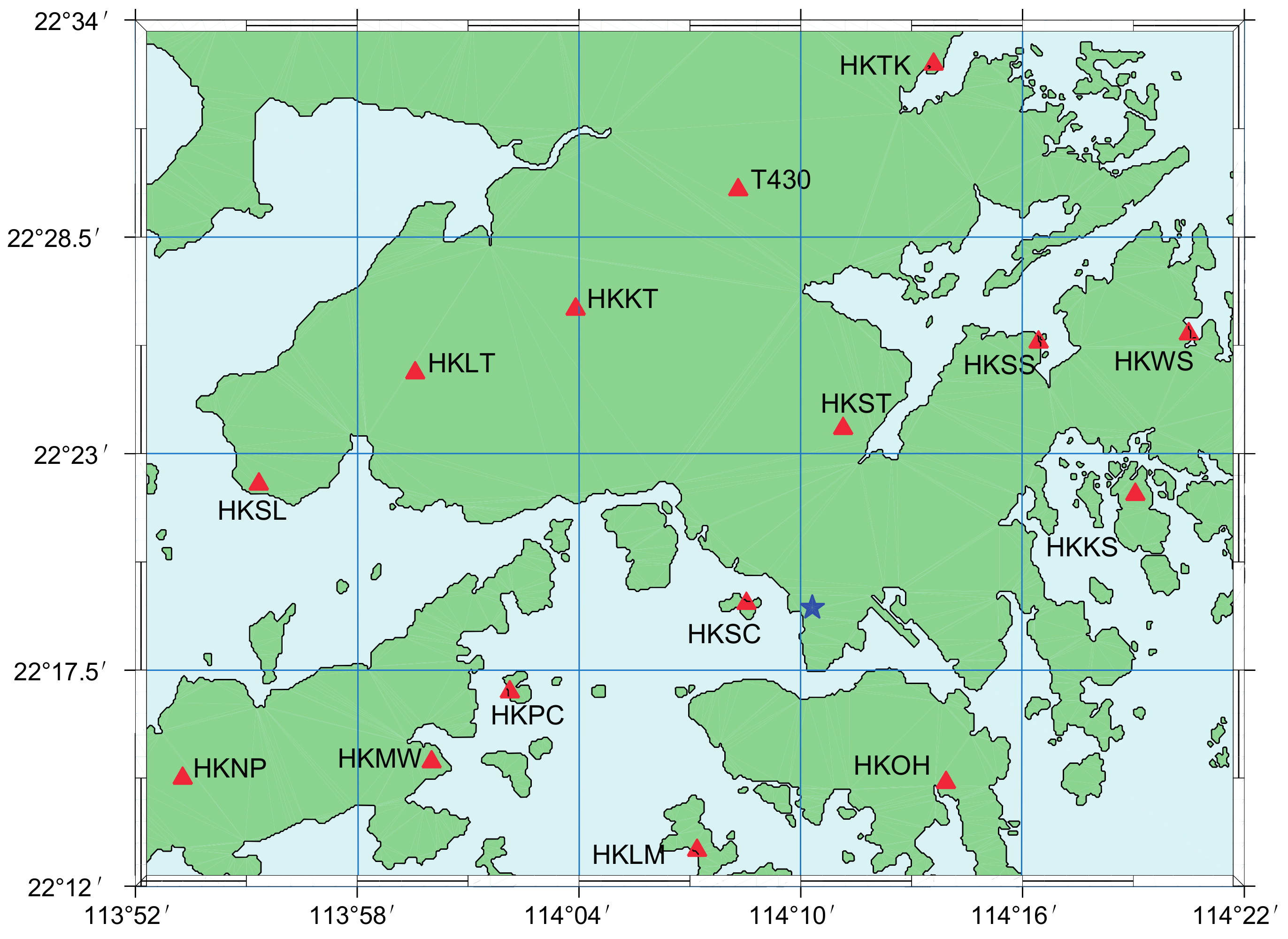
Figure 2.
Three situations in Laplacian smoothing. (a) lies in the central part; (b) lies on the boundary but not in the corner; (c) lies in the corner.
Figure 2.
Three situations in Laplacian smoothing. (a) lies in the central part; (b) lies on the boundary but not in the corner; (c) lies in the corner.

Figure 3.
Vertical wet refractivity from radiosonde data, ALS method and CLS constrained results. (a–n): WR results during rainy period; (o–bb): WR results during rainless period.
Figure 3.
Vertical wet refractivity from radiosonde data, ALS method and CLS constrained results. (a–n): WR results during rainy period; (o–bb): WR results during rainless period.
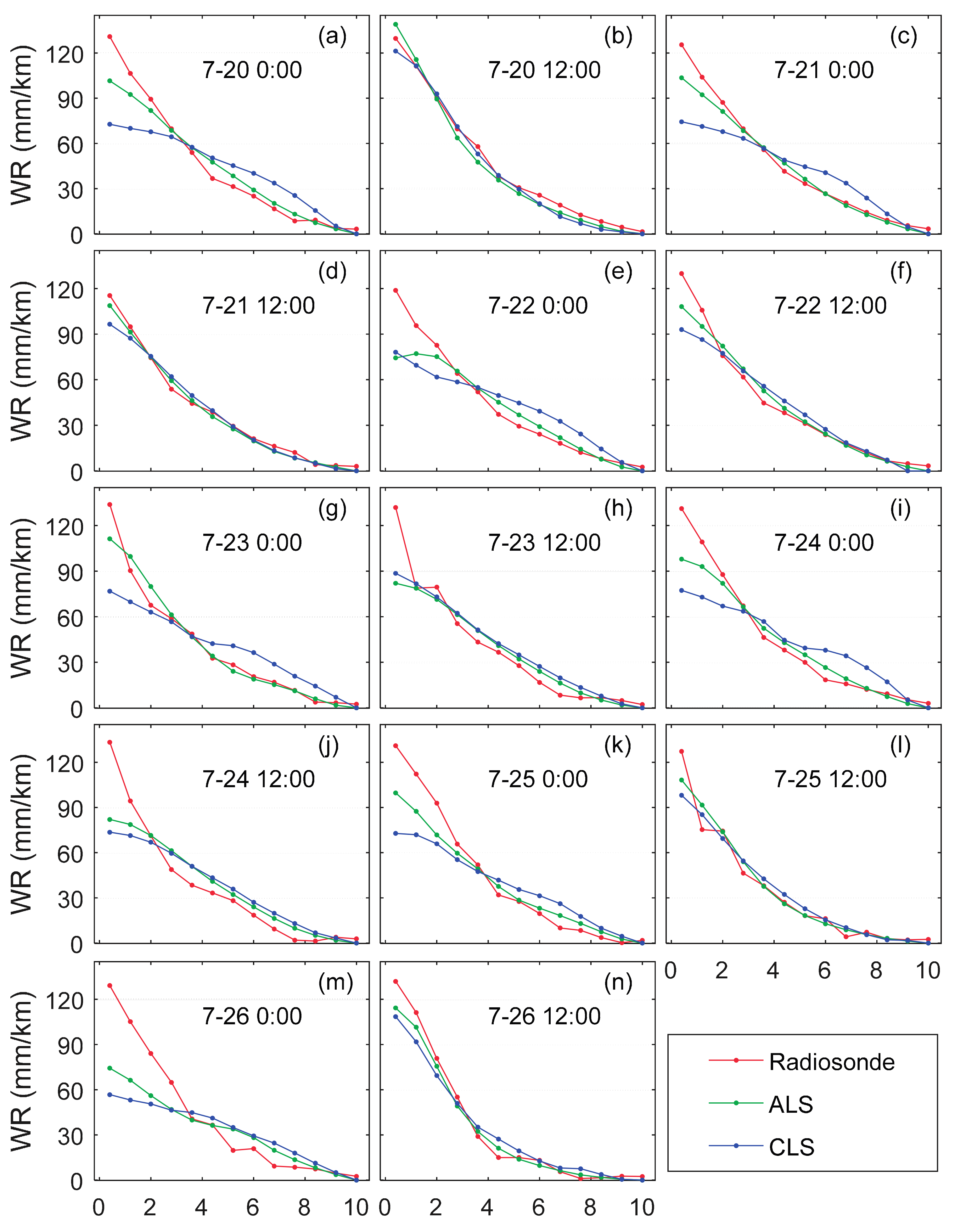

Figure 4.
Comparisons between the tomography results and radiosonde results during 20 July to 26 July. Green lines indicate the a priori information free strategy; Blue lines indicate the one radiosonde constrained strategy; Cyan lines indicate the GNSS meteorological data constrained strategy. (a–n): comparisons between WR at different time points.

Figure 5.
Comparisons between the tomography results and radiosonde results during 1 August to 7 August. Green lines indicate the a priori information free strategy; Blue lines indicate the one radiosonde constrained strategy; Cyan lines indicate the GNSS meteorological data constrained strategy. (a–n): comparisons between WR at different time points.

Figure 6.
Layered bias and STD calculated from the comparison between the tomography results and radiosonde results during rainy days (20 July to 26 July) and rainless days (1 August to 7 August) in 2015. The light blue squares indicate bias and the error bars indicate STD. (a,b): a priori information free strategy; (c,d): one radiosonde observation constrained strategy; (e,f): GNSS meteorological data constrained strategy.

Figure 7.
Layered bias and STD calculated from the comparison between tomography results and ECMWF results during rainy days (20 July to 26 July) and rainless days (1 August to 7 August) in 2015. The light blue squares indicate bias and the error bars indicate STD. (a,b): a priori information free strategy; (c,d): one radiosonde observation constrained strategy; (e,f): GNSS meteorological data constrained strategy.

Figure 8.
Wet refractivity from GNSS meteorological data, radiosonde and ECMWF at 0:00 UTC on 20 July 2015. (a) WR from ground GNSS meteorological data and RS; (b) GNSS meteorological data and RS data derived WR reduced to 400 m height; (c) ECMWF and RS WR reduced to 400 m height.
Figure 8.
Wet refractivity from GNSS meteorological data, radiosonde and ECMWF at 0:00 UTC on 20 July 2015. (a) WR from ground GNSS meteorological data and RS; (b) GNSS meteorological data and RS data derived WR reduced to 400 m height; (c) ECMWF and RS WR reduced to 400 m height.

Table 1.
Statistics of the tomography accuracy with respect to radiosonde data during a rainy period and a rainless period in 2015. unit: mm/km.
Table 1.
Statistics of the tomography accuracy with respect to radiosonde data during a rainy period and a rainless period in 2015. unit: mm/km.
| A Priori Data | Rainy Period | Rainless Period | |||||
|---|---|---|---|---|---|---|---|
| Bias | STD | RMSE | Bias | STD | RMSE | ||
| Low (<5.6 km) | No | −4.9 | 12.6 | 13.8 | −3.2 | 13.0 | 13.6 |
| Lowest radiosonde observation | −1.8 | 5.5 | 6.6 | 0.3 | 7.9 | 8.2 | |
| GNSS meteorological data | −1.6 | 7.2 | 8.4 | 0.9 | 9.0 | 9.4 | |
| Total | No | −2.5 | 10.0 | 10.5 | −0.8 | 10.2 | 10.3 |
| Lowest radiosonde observation | −1.9 | 4.9 | 5.7 | −0.6 | 6.2 | 6.4 | |
| GNSS meteorological data | −2.3 | 5.9 | 6.8 | −0.6 | 7.2 | 7.3 | |
Table 2.
Statistics of the tomography accuracy with respect to ECMWF data during a rainy period and a rainless period in 2015. unit: mm/km.
Table 2.
Statistics of the tomography accuracy with respect to ECMWF data during a rainy period and a rainless period in 2015. unit: mm/km.
| A Priori Data | Rainy Period | Rainless Period | |||||
|---|---|---|---|---|---|---|---|
| Bias | STD | RMSE | Bias | STD | RMSE | ||
| Low (<5.6 km) | No | −1.7 | 10.5 | 10.7 | −2.2 | 11.6 | 12.1 |
| Lowest radiosonde observation | −1.3 | 6.5 | 7.1 | −0.2 | 7.7 | 8.3 | |
| GNSS meteorological data | −0.9 | 6.9 | 7.3 | 0.4 | 7.8 | 8.4 | |
| Total | No | −0.7 | 7.9 | 8.1 | −0.5 | 8.9 | 9.0 |
| Lowest radiosonde observation | −1.7 | 5.3 | 5.7 | −1.3 | 6.2 | 6.5 | |
| GNSS meteorological data | −2.1 | 5.4 | 6.0 | −1.4 | 6.4 | 6.8 | |
© 2017 by the authors. Licensee MDPI, Basel, Switzerland. This article is an open access article distributed under the terms and conditions of the Creative Commons Attribution (CC BY) license (http://creativecommons.org/licenses/by/4.0/).
Share and Cite
MDPI and ACS Style
Zhang, B.; Fan, Q.; Yao, Y.; Xu, C.; Li, X. An Improved Tomography Approach Based on Adaptive Smoothing and Ground Meteorological Observations. Remote Sens. 2017, 9, 886. https://doi.org/10.3390/rs9090886
AMA Style
Zhang B, Fan Q, Yao Y, Xu C, Li X. An Improved Tomography Approach Based on Adaptive Smoothing and Ground Meteorological Observations. Remote Sensing. 2017; 9(9):886. https://doi.org/10.3390/rs9090886
Chicago/Turabian StyleZhang, Bao, Qingbiao Fan, Yibin Yao, Caijun Xu, and Xingxing Li. 2017. "An Improved Tomography Approach Based on Adaptive Smoothing and Ground Meteorological Observations" Remote Sensing 9, no. 9: 886. https://doi.org/10.3390/rs9090886
Note that from the first issue of 2016, this journal uses article numbers instead of page numbers. See further details here.