Determining the Pixel-to-Pixel Uncertainty in Satellite-Derived SST Fields

1
Department of Marine Technology, College of Information Science and Engineering, Ocean University of China, 238 Songling Road, Qingdao 266100, China
2
Graduate School of Oceanography, University of Rhode Island, 215 South Ferry Road, Narragansett, RI 02882, USA
3
Qian Xuesen Laboratory of Space Technology, China Academy of Space Technology, 104 Youyi Road, Beijing 100094, China
4
Laboratory for Regional Oceanography and Numerical Modeling, Qingdao National Laboratory for Marine Science and Technology, 1 Wenhai Road, Qingdao 266237, China
*
Author to whom correspondence should be addressed.
Remote Sens. 2017, 9(9), 877; https://doi.org/10.3390/rs9090877
Submission received: 18 July 2017
/
Revised: 21 August 2017
/
Accepted: 22 August 2017
/
Published: 23 August 2017
(This article belongs to the Special Issue Sea Surface Temperature Retrievals from Remote Sensing)
Abstract
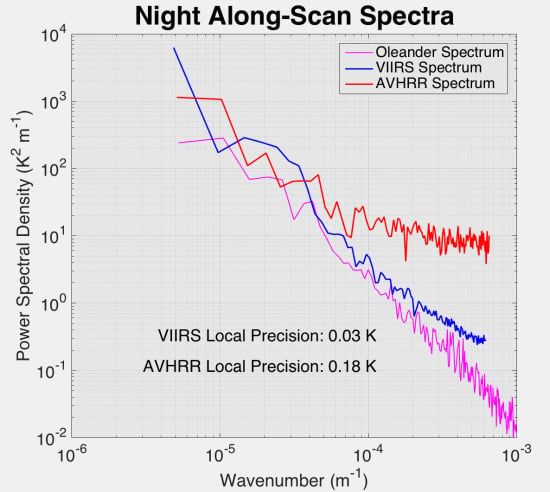
:The primary measure of the quality of sea surface temperature (SST) fields obtained from satellite-borne infrared sensors has been the bias and variance of matchups with co-located in-situ values. Because such matchups tend to be widely separated, these bias and variance estimates are not necessarily a good measure of small scale (several pixels) gradients in these fields because one of the primary contributors to the uncertainty in satellite retrievals is atmospheric contamination, which tends to have large spatial scales compared with the pixel separation of infrared sensors. Hence, there is not a good measure to use in selecting SST fields appropriate for the study of submesoscale processes and, in particular, of processes associated with near-surface fronts, both of which have recently seen a rapid increase in interest. In this study, two methods are examined to address this problem, one based on spectra of the SST data and the other on their variograms. To evaluate the methods, instrument noise was estimated in Level-2 Visible-Infrared Imager-Radiometer Suite (VIIRS) and Advanced Very High Resolution Radiometer (AVHRR) SST fields of the Sargasso Sea. The two methods provided very nearly identical results for AVHRR: along-scan values of approximately 0.18 K for both day and night and along-track values of 0.21 K for day and night. By contrast, the instrument noise estimated for VIIRS varied by method, scan geometry and day-night. Specifically, daytime, along-scan (along-track), spectral estimates were found to be approximately 0.05 K (0.08 K) and the corresponding nighttime values of 0.02 K (0.03 K). Daytime estimates based on the variogram were found to be 0.08 K (0.10 K) with the corresponding nighttime values of 0.04 K (0.06 K). Taken together, AVHRR instrument noise is significantly larger than VIIRS instrument noise, along-track noise is larger than along-scan noise and daytime levels are higher than nighttime levels. Given the similarity of results and the less stringent preprocessing requirements, the variogram is the preferred method, although there is a suggestion that this approach overestimates the noise for high quality data in dynamically quiet regions. Finally, simulations of the impact of noise on the determination of SST gradients show that on average the gradient magnitude for typical ocean gradients will be accurately estimated with VIIRS but substantially overestimated with AVHRR.
1. Introduction
To date, a great deal of attention has been focused on the accuracy of satellite-derived sea surface temperature (SST) products (see, for example, [1,2,3,4,5], a very small fraction of the articles addressing this issue). By contrast, the spatial precision (defined below) of satellite-derived SST fields has only been addressed by Tandeo et al. [6] (Tan14 hereafter), and that peripherally in an analysis of the anisotropy of SST fields in the global ocean. Donlon et al. [7] provide an excellent overview of the general approach (based on the bias and variance of pixel SST values relative to co-located in situ values) used to determine satellite data product accuracy. A feature of this approach is that the satellite–in situ matchups are generally widely separated in space and time, because of cloud cover and the paucity of in situ data. This often results in a spatially slowly varying bias in the retrieved SST values, because a significant contribution to the uncertainty in satellite retrievals results from atmospheric contamination, the spatial scales of which are, in general, large compared with the pixel separation of infrared sensors. This means that the pixel-to-pixel uncertainty, the spatial precision, may be substantially smaller than the accuracy determined from in situ match-ups. Indeed, Tan14 estimates the spatial precision of Advanced Very High Resolution Radiometer (AVHRR) to be approximately 0.2 K, substantially smaller than the estimated accuracy of 0.5 K [1,2,3] and, as will be shown in the following, the difference between the spatial precision and the accuracy of Visible-Infrared Imager-Radiometer Suite (VIIRS) SST fields is even more pronounced, 0.08 K versus 0.4 K [4,5]. The lack of knowledge related to the spatial precision of satellite-derived SST fields makes selection of the appropriate dataset as well as the combination of datasets derived from different sources problematic at best for studies of processes at the one to ten pixel spatial scale.
We refer to the uncertainty of the retrieved SST relative to the actual SST as the values accuracy. By contrast, we refer to the uncertainty in SST following removal of a bias in the field associated with long-wavelength phenomena as the spatial precision of the field. The latter is important in studies related to the SST gradient, while the former to processes for which the specific value is important, such as those directly related to air–sea fluxes of a variety of properties. One might also refer to the temporal precision of the retrievals—the uncertainty of SST retrievals at a given location between consecutive satellite passes of the sensor from which the fields are being derived. However, the time scale separating consecutive retrievals for most satellite-borne infrared sensors is large relative to the time scale associated with atmospheric phenomena, hence the temporal precision will be close to the accuracy as described above.
In this study, we investigate the spatial precision of Level-2 (L2) [8] SST fields obtained from the VIIRS carried on the Suomi-National Polar-orbiting Partnership (Suomi-NPP) spacecraft launched in October 2012 and L2 SST fields obtained from the AVHRR carried on NOAA-15. Note that Tan14’s estimate of spatial precision is based on comparisons with L3 fields, adding a processing step that is likely to add additional error to the fields. VIIRS fields were selected because of their high spatial precision as will be shown in Section 5.1. AVHRR fields were chosen because AVHRR instruments comprise the longest, global satellite-derived SST record, dating back to late 1981. L2 data were selected because they form the basis of all higher order products obtained from these sensors, hence provide a lower limit for the small-scale retrieval noise to be expected in their products. The contribution of instrument noise to the spatial precision for each of these datasets will be determined using two methods, one based on spectra, the other on variograms of the fields [6].
In Section 2, we describe the datasets, the study area and the period covered by the analysis. This is followed in Section 3 by a discussion of the preprocessing of the datasets and then of the two approaches used to estimate the “instrument” noise and from that the spatial precision under cloud-free conditions. The results of the analyses are in Section 4 and the related discussions are in Section 5.
However, first, we describe the error budget associated with satellite-derived SST fields.
The Error Budget of Satellite-Derived SST Fields
A number of factors contribute to the uncertainty in satellite-derived SST fields. These are described in a White Paper prepared by the National Aeronautics and Space Administration (NASA)-National Oceanic and Atmospheric Administration (NOAA) SST Science Team [9] and summarized in Figure 1. Although the accuracy of an L2 skin temperature dataset is determined by the accumulation of the error elements shown in the upper gray box of Figure 1, which also shows the relationship between these errors and the level of processing, it is generally dominated by contributions from the atmosphere—the green block. As noted above, atmospheric retrieval errors tend to be long wavelength, with an e-folding distance of many pixels in the case of infrared retrievals. The spatial precision, on the other hand, is dominated by instrument noise and classification errors (e.g., cloud-contaminated pixels passing as clear pixels) for skin temperature L2 and L3U datasets. (In the case of “buoy” temperature L2 and L3U datasets, the error in extrapolating from the skin temperature, the quantity actually measured by the satellite, to the temperature at the depth of the buoy, generally 1 m below the surface, additional contributions to the spatial precision may result from the horizontal variability in the vertical temperature step, the orange block in the figure. Only L2 skin temperature SST fields are considered in this study, hence horizontal gradients in the surface to buoy depth temperature difference do not contribute to the uncertainty in retrievals discussed herein.) For L3C, L3S and L4 datasets, the collation and interpolation schemes used will likely contribute to a decrease in spatial precision—an increase in the pixel-to-pixel errors—but the degree to which this is the case has yet to be documented. Important in the analysis presented herein is the distinction between instrument noise (elements in the yellow block of Figure 1) and the noise associated with classification errors (one of the elements in the green block). Classification errors generally refer to the improper masking of cloud-contaminated pixels and this misclassification is thought to be dependent on cloud cover—the larger the fraction of the area contaminated by clouds, the larger the fraction of misclassified pixels. The contribution of misclassified pixels to the local error is also likely to depend on cloud type. Together, these observations suggest that the classification error may vary significantly geographically. For this reason, our focus is on instrument noise, which we assume to be less dependent on location, i.e., the estimates of instrument noise obtained in this work are thought to be good estimates in regions of low cloud cover and a lower bound in general.
2. Data
This study makes use of one dataset consisting of thermosalinograph (TEX) sections, one L2 SST dataset obtained from VIIRS radiances and one L2 SST dataset obtained from AVHRR radiances. These are discussed below along with the study area and period.
2.1. In Situ Temperature
The thermosalinograph, on which the in situ data are based, was mounted on the MV Oleander, a container ship making weekly round trips between Port Elizabeth, NJ, USA and Hamilton Harbor, Bermuda (Figure 2). Thermosalinograph temperature measurements were obtained from two thermistors, one from the seawater intake in the interior of the ship and the second directly at the intake, i.e., “external” to the hull. The exterior measure (referred to as TEX for “exterior” temperatures) is thought to be the most accurate [10] (Sch16 hereafter), hence only these are used in the work presented here. The SBE38 remote temperature sensor, on which the TEX data are based, has an accuracy of 0.0001 K, a resolution of 0.00025 K (although the TEX instrument noise is estimated to be 0.00069 K based on the variogram approach discussed in Section 3.3), and a response time of 0.5 s. The TEX sensor sampled every 10 s resulting in an approximate spatial resolution of 75 m at the typical 16 knots cruise speed of the Oleander. TEX data for the period September 2007 to fall 2013 were obtained from the Atlantic Oceanographic and Meteorological Laboratory. The quality control procedures used to screen these data are described in Sch16.
2.2. Visible-Infrared Imager-Radiometer Suite (VIIRS)
The L2 VIIRS SST retrievals used here were derived from the VIIRS “Moderate Resolution Bands”, which have a resolution of approximately 750 m at nadir. Because of the way in which the instrument samples, the resolution decreases very slowly (compared with other satellite-borne instruments, Figure 3) to approximately 1600 m at the scan edge, a ground distance of approximately 1500 km from nadir [11,12].
For this study, we used the VIIRS SST product obtained from NOAA’s Comprehensive Large Array-data Stewardship System (the VIIRS Sea Surface Temperature Environmental Data Record (EDR) obtained from: http://www.nsof.class.noaa.gov/saa/products/search?datatype_family=VIIRS_EDR) produced with the Joint Polar Satellite System (JPSS). Only quality level 1 data, the “best” quality level, were used. Although screening at this level ideally removes all cloud contaminated pixels, some are still included in the analysis, leading to the misclassification error discussed above.
2.3. AVHRR Pathfinder SST
The AVHRR product used was derived with the Pathfinder retrieval algorithm developed at the University of Miami [13]. The algorithm was applied to the High Resolution Picture Transmission (HRPT) data stream obtained from the AVHRR on NOAA-15. Retrievals were performed at the University of Rhode Island. Only pixels with a quality level of 3 or higher were used. The nominal pixel spacing is 1.1 km although, as can be seen in Figure 3, it increases significantly from this value. This increase is what motivated use of pixels within 500 km of nadir as discussed below.
2.4. The Study Area
MV Oleander traverses several distinct dynamical regimes: the shelf, the Slope Sea, the Gulf Stream, and the Sargasso Sea. In that the focus of this analysis is on the spatial resolving power of satellite-derived SST datasets, it is important to select a region in which the geophysical variability of the SST field does not overwhelm the uncertainty associated with the SST retrievals, be they driven by misclassification errors (the green block in Figure 1) or instrument/calibration issues (the yellow block). Specifically, this means selecting a dynamically “quiet” region in the ocean. The Sargasso Sea portion of the Oleander track between 32°N and 36°N meets this requirement. In order to increase the amount of satellite-derived data used in our analysis, we consider all data in the region between 63°W and 72°W, and 32°N and 36°N (Figure 2). This region was selected with the expectation that the dynamics are similar to those seen along Oleander track between 32°N and 36°N hence the spectra should be similar in both slope and energy. As shown in Sch16, spectra including the Gulf Stream are substantially more energetic than those for SST in the Sargasso Sea.
2.5. The Study Period
The analyses presented here are based on SST fields from the summer of 2012 only—June, July and August. Sch16 show that spring (March, April and May) and summer spectra tend to be about twice as energetic, over the spectral range examined, 1 to 100 km, as fall and winter spectra suggesting that the latter would be more appropriate for the evaluation proposed here, but the summer months are also substantially less cloud contaminated than the other seasons. Furthermore, the increased spectral energy is likely due in part to diurnal warming, the effect of which may be mitigated by selecting nighttime fields only as shown in Section 4.2. This raises a concern with regard to the TEX data because TEX sections are not synoptic, taking approximately 20 h to cross the study area. However, since the TEX samples between 5 and 6 m below the surface, diurnal warming is not thought to be a significant problem [14].
3. Methodology
3.1. The Spectral Approach
The spectral method, to determine retrieval noise at the pixel level, is based on an analysis of the large wavenumber tail of the power spectral density of SST temperature sections extracted from the SST fields. Spectra are based on the Discrete Fourier Transform (DFT) determined from the Fast Fourier Transform (FFT) (see Sch16 or Wang et al. [15], who also used the DFT to analyze TEX spectra). The FFT requires equally spaced, gap-free data, i.e., gaps, if they exist in the original series, must be filled and the data must be interpolated to equal spacing, if not already equally spaced, prior to applying the FFT algorithm. For satellite-derived fields, gaps result from cloud cover, intervening land values (not an issue for the region studied here) or missing scans while pixel spacing depends on the product. (The filling of gaps is discussed in Section 3.1.1.) In the case of L2 products the spacing of pixels in the along-scan direction varies with distance from nadir (Figure 3), as does the along-track spacing, although much less so (<0.5% change from nadir to the swath edge for both AVHRR and VIIRS). For the in situ data, intermittent system failures resulted in gaps although not to the extent of those in the satellite data and sample spacing depends on the ship speed, which varies.
Of importance to the analysis presented here is that interpolation, either to fill gaps or to regularize the spacing of samples on a section, impacts the resulting spectrum, with the impact generally increasing as the wavenumber increases, i.e., in the spatial range of most importance to the analysis here. Furthermore, the impact is a function both of the fraction of “good” values (defined as by Sch16), and the degree to which the “missing” data are clustered (referred to as cohesion and assigned the symbol [16]). Sch16 found that “…spectral slopes are increasingly biased low as decreases and increases, and this effect becomes more pronounced as the true spectral slope increases”. Based on this they only considered VIIRS spectra for and in their analysis. We found these thresholds to be too permissive for our purposes; the impact of interpolation on spectra in the 1 to 10 pixel range can overwhelm the underlying spectrum as will be shown below. We therefore chose more stringent constraints on , generally resulting in . At this level, the cohesion of the data has a relatively small impact on the spectra for slopes in the range of those observed in the Sargasso Sea [10], so we did not impose an additional constraint on cohesion.
3.1.1. Selection of the Sections
Satellite-Derived Fields. The satellite-derived SST fields evaluated here are obtained from scanning radiometers, the characteristics of which may differ in the along-scan versus along-track directions. This is indeed the case for VIIRS due to the use of multiple detectors for each scan, which results in striping of the fields [17]. The decision was therefore made to separate the data into along-scan and along-track sections. The data were farther divided into day and night fields to allow analysis of the possible effect of diurnal warming on the spectral characteristics of the fields. This is of particular importance given the selection of the Sargasso Sea in summer months, a period when diurnal warming is significant [18].
Also with regard to the selection of sections from the L2 datasets is their distance from nadir. Both the area of each pixel (approximately the along-track spacing, 741 m for VIIRS and 1115 m for AVHRR, times the along-scan spacing) and the spacing of pixels along the scan increases away from nadir (Figure 3). Both of these factors impact along-scan spectra at small scales, while the increase in pixel size impacts along-track spectra, again at these scales. Although the pixel spacing of along-track sections is virtually independent of the distance from nadir, the size of the pixel is not, i.e., the SST values associated with pixels is averaged over increasingly larger areas away from nadir. This is similar to smoothing along-track with a moving average, which in turn depresses the power spectral density at small scales, this, independent of the preprocessing performed on the data and it affects along-track and along-scan spectra equally. Along-track interpolation (discussed below) to address the change in pixel spacing in the along-scan direction (Figure 3) also impacts the resulting spectra. In order to reduce the impact of both of these effects, only sections within 500 km of nadir are used for this analysis.
The final criterion used to select sections from the L2 fields relates to the gappiness of the data. For clarity, we combine this step with the interpolation to fill missing pixel values in the study area. The actual implementation of the algorithm is slightly different, to reduce processing time, but the result is the same. Missing values in the study area were replaced using a Barnes filter if 13 of the 24 pixels in a 5 × 5 pixel square surrounding the pixel of interest are cloud-free, otherwise the pixel remains flagged as missing. This corresponds to a decay scale associated with the averaging of 1.5 km for VIIRS and 2 km for AVHRR and follows the approach taken by Sch16. Following this gap filling, all complete (no missing values) 256 pixel, non-overlapping sections in the along-track direction meeting the distance from nadir criterion were selected as were all non-overlapping along-scan sections. Only a small fraction of sections used in the final analysis had more than 15 missing pixels in the original data (more than 6% of the pixels were filled on <10% sections). The impact of this on the final spectra was evaluated for the worst case scenario by using the Barnes filter to fill every point on a section (gap filling was still possible in that adjacent pixels were left as is, i.e., not set to missing values), not just the pixels with missing values. The result suggests that the gap filling performed only for pixels with missing values has little impact on the final spectra, because the number of missing values is in general small; less than 0.6% of all values contributing were replaced with the Barnes filter.
Oleander Sections. Only TEX sections that met the selection criteria of Sch16 were considered. Of these only sections with a maximum pixel separation of 150 m in the Sargasso Sea were selected. (Selection of temperature sections with maximum sample spacing in excess of 150 m resulted in a significant steepening of the spectral slope for wavelengths smaller than approximately 1 km. This is due to the nearest neighbor interpolation to 75 m spacing, which repeats samples for these large separations.) Barnes filtering with a decay scale of 0.2 km was used to fill these gaps and the resulting sections were nearest neighbor interpolated to a mean spacing of 74.9 m, the mean spacing averaged over all sections; the mean spacing varies from section-to-section with a minimum of 74.6 m and a maximum of 75.0 m [19].
Table 1 lists the number of satellite-derived sections by along-scan/along-track, day/night combination for the summer (June–August) of 2012 and the number of Oleander TEX sections for the summers of 2008–2013.
3.1.2. Interpolation to Equal Spacing
Satellite-Derived Fields. As previously noted the pixel separation in the along-scan direction changes with distance from nadir. Because the spectral energy determined with the standard FFT is a function of pixel spacing and the number of pixels in the section, combining data with different spatial resolutions tends to add noise to the spectra. To address this, along-scan sections were divided into three groups each for VIIRS and AVHRR based on mean pixel spacing. First, all adjacent temperature sections for a given satellite pass were grouped into subgroups and the mean separation of pixels for the subgroup was calculated (The subgroups ranged in size from 1 to O (100) sections depending on cloud cover.). Each subgroup was then assigned to the group indicated in Table 2 based on the mean pixel spacing of the subgroup. All of the temperature sections falling in a given group were then interpolated to the same pixel spacing, also shown in Table 2. This pixel spacing was determined from the mean pixel spacing determined from the contributing temperature sections for the given group. This, together with the relatively small size of the ranges, tended to eliminate problems associated with different spatial sampling and with an interference between the sampling frequency along the original section and that along the interpolated section. Nearest neighbor interpolation was used. Figure 4 shows the effective transfer function of three different interpolation algorithms available in Matlab: linear, nearest neighbor and cubic spline. To determine the most appropriate resampling strategy, SST values on the VIIRS sections were replaced with white noise and interpolated. Linear interpolation smooths the field the most resulting in a significant loss of energy at small wavelengths, the portion of the spectrum of most interest here. Cubic spline does better but still results in a loss of energy at small wavelengths. Nearest neighbor interpolation does not significantly alter the distribution of values but does alter the effective wavelength—by shifting the values in space. However, the effect on the spectrum is small since the values have been shifted to locations, which are on average relatively close to the original values—the use of the mean spacing of pixels (which varies from group-to-group) rather than a fixed spacing for all sections.
3.1.3. Detrending
Typically, a windowing function is applied to time series (or temperature sections in this case) prior to obtaining the spectrum so as to reduce leakage between frequencies and the introduction of spectral energy due to step changes at the ends of the section. However, windowing functions tend to depress the amount of energy in the spectrum, which results in an underestimate of the instrument noise, so we elected not to window the data. Specifically, several different windowing functions, as well as simple detrending, were applied to simulations generated by adding white noise to randomly generated temperature sections with a linear power spectral density (in log-log space) typical of the spectra obtained from the SST sections but with random phase of the spectral elements between −π and +π. Detrending provided the most accurate estimate of the imposed noise when compared to analysis of the data with the various windowing functions or to analysis of the data with no preprocessing.
3.1.4. FFT
Finally, the FFT function available in Matlab was used to obtain the spectra from the detrended temperature sections. For the along-scan direction, power spectral densities were ensemble averaged over each of the subgroups defined in Section 3.1.1. This resulted in approximately 100 subgroups for all groups of the AVHRR/VIIRS, day/night combinations, i.e., there was an average of eight subgroups for each of the defined groups. Similar averaging was performed for the subgroups of the along-track direction.
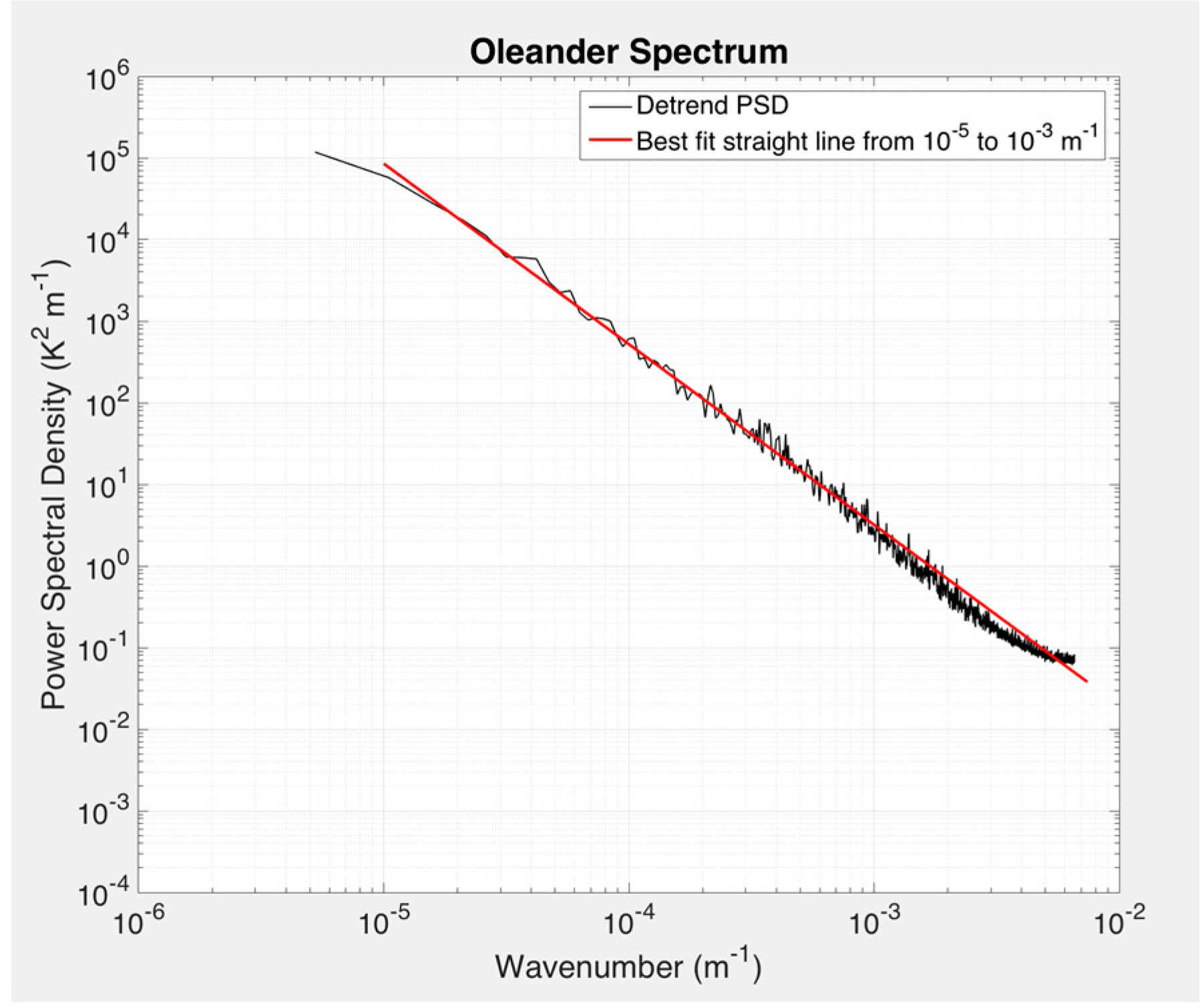
Oleander spectra were ensemble averaged over all of the selected sections.
3.2. Estimation of Instrument Noise
Instrument noise in the satellite-derived fields is estimated from the shape of the power spectral density on the short wavelength (large wavenumber) end of the retrieved spectra. To better understand the approach, consider the factors contributing to this portion of the spectrum. If adjacent values on a given temperature section are independent with no noise, then the shape of the spectrum is defined by the geophysical processes in the region. If the field has been smoothed or averaged over a significant region, there is little additional information in the value of one point relative to an adjacent one and the spectrum falls off more rapidly than the shape associated with geophysical processes. This is what we found for the spectra of the AVHRR SST fields associated with large scan angles (not shown here) as well as with the oversampled TEX sections with maximum spacing of samples in excess of 150 m resampled to a spacing of 75 m discussed in Section 3.1.1. To avoid the roll-off of the spectra at small wavelengths the data were not smoothed. If the field is not smoothed and, white noise is added to the values at individual pixels, the spectrum will tend to level off; the point at which it begins to do so being a function of the level of the added noise. Finally, if energy remains in the geophysical spectrum at wavenumbers larger than those at the end of the retrieved satellite-derived spectra, the spectra will also tend to level off near their end as a result of energy aliased from the larger wavenumbers. This is likely the reason the ensemble averaged Oleander TEX spectrum levels off (Figure 5). (It is not clear whether the slight fall off in the TEX spectrum beginning at approximately 1 km is a result of a fall-off in the geophysical signal or some form of averaging of the TEX data. However, this roll-off is very slight and ignored here.) In summary, the large wavenumber tail of the satellite-derived spectra is subject to the following:
- An increase in the magnitude of the slope of the spectrum due to averaging over the footprint of the sensor;
- A decrease in the slope due to geophysical noise aliased into the spectrum, especially at high wavenumbers; and
- A decrease in the slope due to instrument noise, the quantity of interest here.
In order to determine the instrument noise, i.e., to separate it from the other factors cited above, we defined a two-step process based on the following three assumptions:
- log10 of the geophysical power spectral density in the study area falls off linearly with log10 of the wavenumber over the spectral range sampled by the satellite-borne sensors (1.5 to order 100 km).
- The spectrum continues to roll-off with approximately the same slope, at wavenumbers larger than those associated with the Nyquist frequency of the satellite temperature sections. This and the previous assumption are borne out by the mean TEX spectrum shown in Figure 5 as well as from the analysis of the spectra from the two sensors.
- The instrument noise for both sensors is white; i.e., it contributes equally at all wavenumbers associated with the given temperature sections. This is not quite the case for VIIRS hence one has to take a bit more caution with the results presented herein.
In the first step, the slope, intercept and noise level of a hypothetical spectrum yielding the best fit to the satellite spectrum is determined in a least squares sense. This is done by minimizing γ, the sum of the squared difference between the hypothetical spectrum and the satellite spectrum:
where slope and intercept define the straight line portion of the best fit spectrum in log-log space (assumption 1 above), noise is the noise level (assumption 3) also in spectral space, ki is the wavenumber of the ith spectral component and the corresponding power spectral density of the satellite spectrum. In the second step, the constant noise level used to generate the spectrum in Equation (1) is related to white noise in the spatial domain. Specifically, 1000 noise-free temperature sections, with one tenth the sample spacing of that associated with the sensor of interest, are generated by inverse Fourier transforming spectra with the same slope and intercept found with Equation (1) but with the phase of each spectral component randomly selected between −π and π. A 10-point moving average is then applied to each temperature section and the result is decimated by 10. Gaussian white noise of magnitude σ is then added to each point on each section, the sections are Fourier transformed, ensemble averaged and a new figure of merit is obtained:
where is the ensemble averaged power spectral density of the simulated temperature sections and is the best fit power spectral density to the satellite-derived power spectral density based on the slope, intercept and noise found with Equation (1). This is repeated over a range of white noise levels σ to find the level, which best corresponds to the noise level obtained with Equation (1). Of importance, is that generating temperature sections with 1/10 the spacing of the data associated with the sensors of interest, the energy at higher wavenumbers than those resolved by the instrument are aliased into the results thus allowing for a more accurate estimate of the instrument noise. In addition, averaging the oversampled temperature section simulates averaging performed over the footprint of the sensor. However, this does not take into account additional averaging, which takes place in the 2nd dimension of the sensor’s footprint. This is not thought to contribute significantly to the determination of instrument noise outlined above.
3.3. The Variogram Approach
To determine instrument noise from variograms, a model, which includes instrument noise as one of its parameters, is fit to the empirical variogram. The model is intended to reflect the spatial characteristics of the underlying data, hence selection of an appropriate model for the data of interest is critical. Various models have been identified in the literature [20]. Tan14 used an exponential model of the form:
where , referred to as the nugget, is the variance of the difference in the retrieval at a given location from that at a neighboring location as the separation between the two locations goes to zero, i.e., the instrument noise in this case, , referred to as the sill, is the variance associated with the variability for a spatial separation of L, the decorrelation scale. Note that the sill is a measure of the geophysical variance of the field, , plus the “large” scale retrieval variance, which depends on the variance in the atmosphere, the variance of the surface emissivity, instrument noise, etc. So,
where is the total variance of the retrieval.
The formulation used by Tan14 works well for relatively homogeneous datasets for which the underlying variogram has an exponential form [6]. However, in the Sargasso Sea, the shape of the empirical variograms, for the L2 SST fields of interest, differ from subregion-to-subregion, not only in terms of parameters but also in terms of the model itself, with an exponential model fitting in some cases and a Gaussian model in others. In light of this, we have elected to use the “stable semivariogram” [20], a slightly modified single model, of the form:
Note, in comparison to Equation (3), Equation (5) includes an extra parameter, w, which ranges from 1 for the exponential form to 2 for the Gaussian form. Although variograms can be developed in two dimensions for the model of interest, we chose to use variograms for the along-scan and along-track directions separately for much the same reasons presented in the discussion of the preliminary processing of the data,
As in Tan14 we use the formulation given by Cressie to estimate the variogram [21]:
where is at location , Δx or y is the spatial separation in kilometers of pairs in the along-scan (x) and along-track (y) directions, and is the number of such pairs, which varies withand the number of cloud contaminated pixels.
For each of the combinations of interest (along-scan/along-track, day/night), a variogram was obtained (Equation (6)) for each of the interpolated, equally spaced temperature sections used in the spectral approach and described in Section 3.1.1 and Section 3.1.2. Next, for each variogram, the values of , σ, and w of Equation (5), which minimized the weighted squared difference between Equation (5) and the variogram, were obtained. The fit was performed over separations up to 20 km. (The nugget did not vary significantly for fits up to approximately 40 km. However, fitting to a larger range generally resulted in an increase in the nugget, which was thought to be unrealistic—the nugget wandered away from the variance at the smallest observed separation.) The weight assigned to each separation was equal to the number of pairs at that separation over the total number of separations contributing to the variogram, i.e., the weight assigned to a given separation decreased as the separation increased. The best-fit nuggets were then averaged for all temperature sections corresponding to a given sensor/day-night combination to obtain the estimate for instrument noise for that combination. Nuggets were also averaged by the subgroups identified in Section 3.1.1.
4. Results
The spatial precision of satellite-derived SST retrievals, the noise resulting from processes in the yellow and green boxes of Figure 1, which we refer to as instrument noise here, is shown in Table 3 for each of the along-scan/along-track, day/night combinations. The first row for each sensor (labeled Spectra) corresponds to the estimates obtained from the spectral method. Only subgroups consisting of five or more temperature sections and with a spectral slope steeper than −1 were used. The instrument noise for subgroups with shallower spectral slopes tended to dominate the geophysical signal increasing the uncertainty in the fit of Equation (1). The noise estimates provided in the table are the means of the estimates associated with each subgroup. The uncertainty is the square root of the variance of these means over the number of contributing subgroups. Variogram estimates follow in the next row (labeled Variogram) for each sensor. The means of the estimates are from the same subgroups used in the spectral approach and the uncertainties are calculated as for the spectral approach. The final row of the table (labeled Upper Limit) for each sensor is an “upper limit” on the instrument noise assuming that the pixel-to-pixel noise is white. This was obtained by noting that the variance of the difference of adjacent SST values, is the sum of the variances of the noise of each of the two values, , plus the contribution due to the geophysical variance between the two values, :
If the noise is not white, for example, the actual level of noise may, in fact, be larger than the “upper limit”.
4.1. AVHRR
Day-versus-night, along-scan instrument noise levels obtained for the AVHRR data are not statistically distinguishable. Nor are the along-track levels. The levels for the variogram estimates based on the same subgroups as the spectral estimates (2nd row) are also statistically similar. Furthermore, although somewhat larger, the variogram estimates are quite close to the spectral estimates, and all of the estimates are close to the upper limit (Equation (7) ) for the given sensor/day-night/scan-track combination, suggesting that the instrument noise is white. It is possible that the pixel noise is correlated at small scales but, again, the mechanism for this is not obvious.
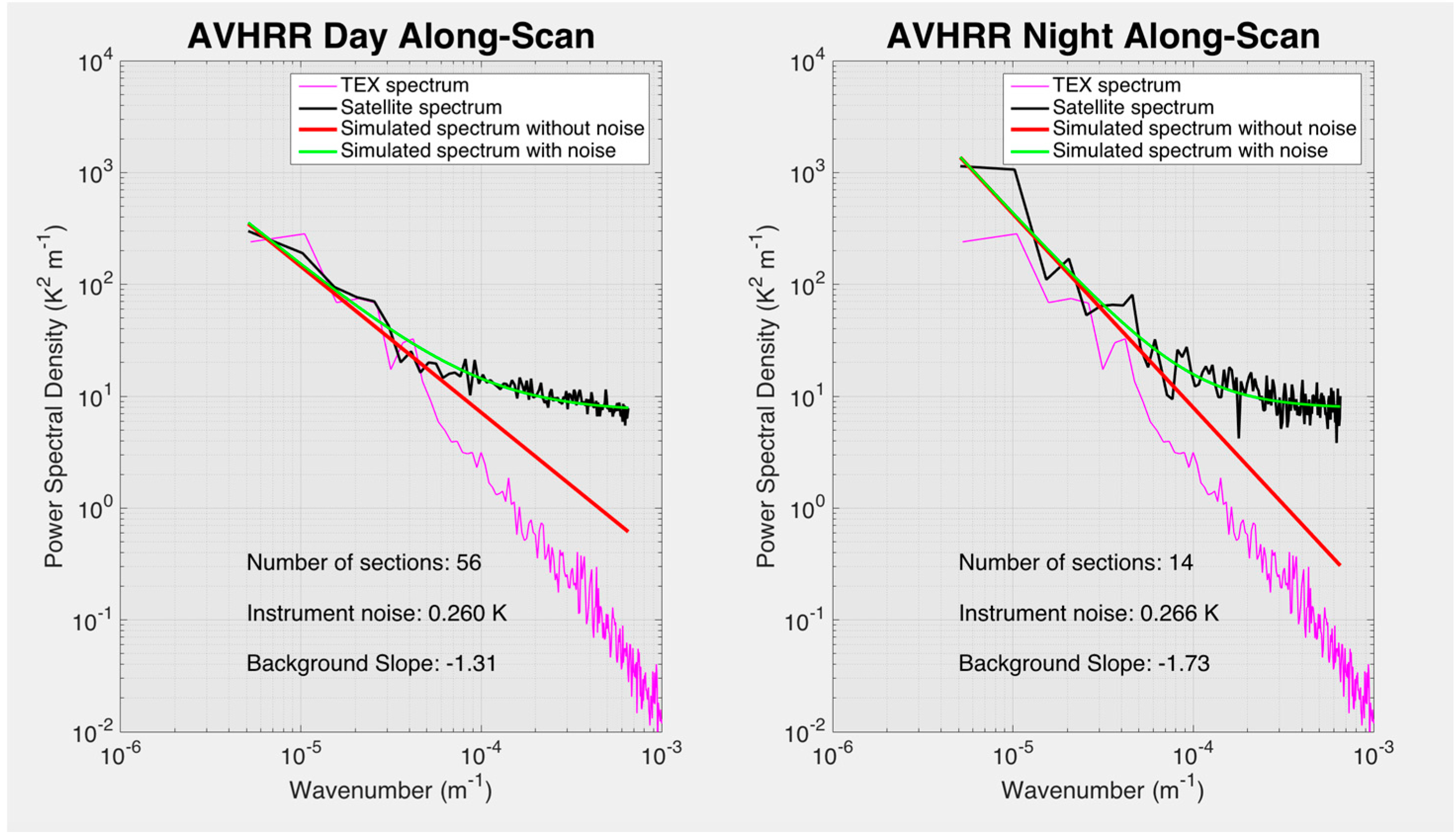
The along-scan AVHRR spectra are shown in Figure 6 for a daytime subgroup and a nighttime subgroup. The best-fit linear spectra with noise are also shown in Figure 6, obtained as discussed in Section 3.2. Figure 7 shows the corresponding along-track AVHRR spectra. In all four cases, noise is seen to impact the spectrum for wavelengths (wavenumbers) up (down) to approximately 25 km (0.04 km−1). The approximately linear portion of the AVHRR spectrum corresponds to a small fraction (~10%) of the 129 spectral values, which is also apparent from these plots. This means that relatively small changes in the low wavenumber end of these spectra will have a more significant impact on the estimated background slope than for spectra less impacted by noise. However, the spectral method for determining instrument noise is relatively insensitive to this; significant changes in slope and intercept result in virtually identical values of instrument noise. For example, for the spectrum shown in the left panel of Figure 7, a slope, offset combination of (−1.7570, −6.2730) yields the same level of instrument noise. This is because the instrument noise is one to two orders of magnitude larger that the assumed geophysical signal, the straight line portion of the spectrum, over a significant fraction of the spectrum (remember the fits are in regular, not log-log space) so changes in the slope do not result in a significant difference in the squared sum of the differences between the model and the observed spectrum. For spectra that level off substantially at large wavenumbers, the noise is effectively determined by the power spectral density level at these wavenumbers. This is readily seen in Figure 6 and Figure 7; the high wavenumber end of the simulated spectra with noise are at a similar level for the along-scan sections and at a slightly higher level for the along-track sections. Care must be taken however when the level of instrument noise is similar, or smaller, in magnitude to the geophysical signal at these wavenumbers, as will become clear in the analysis of the VIIRS spectra.
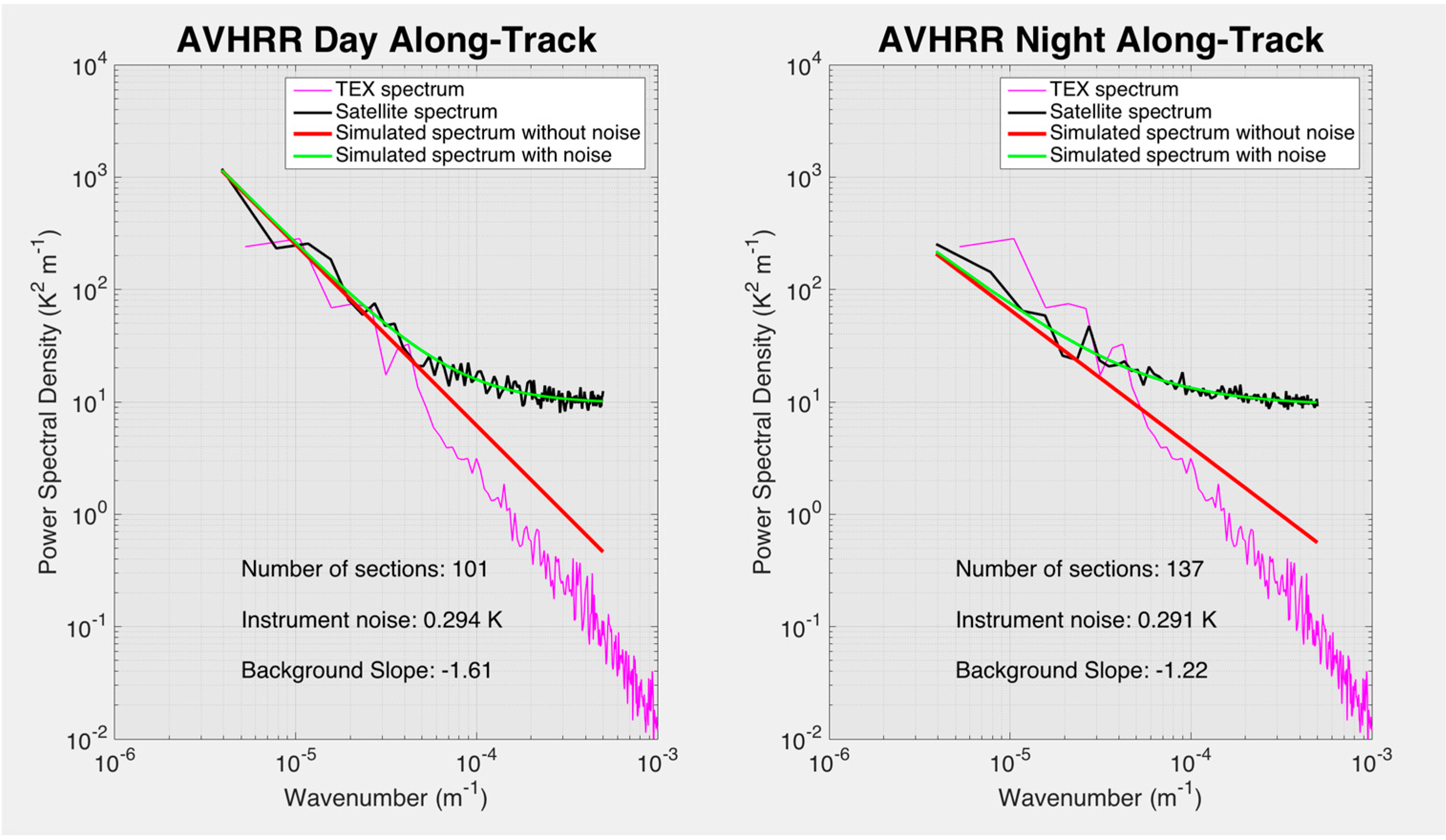
AVHRR along-track instrument noise is approximately 20% larger than along-scan instrument noise. This is presumably due to the line-by-line calibration undertaken in the development of the L1b data product used as input to the L2 retrieval algorithm.
4.2. VIIRS
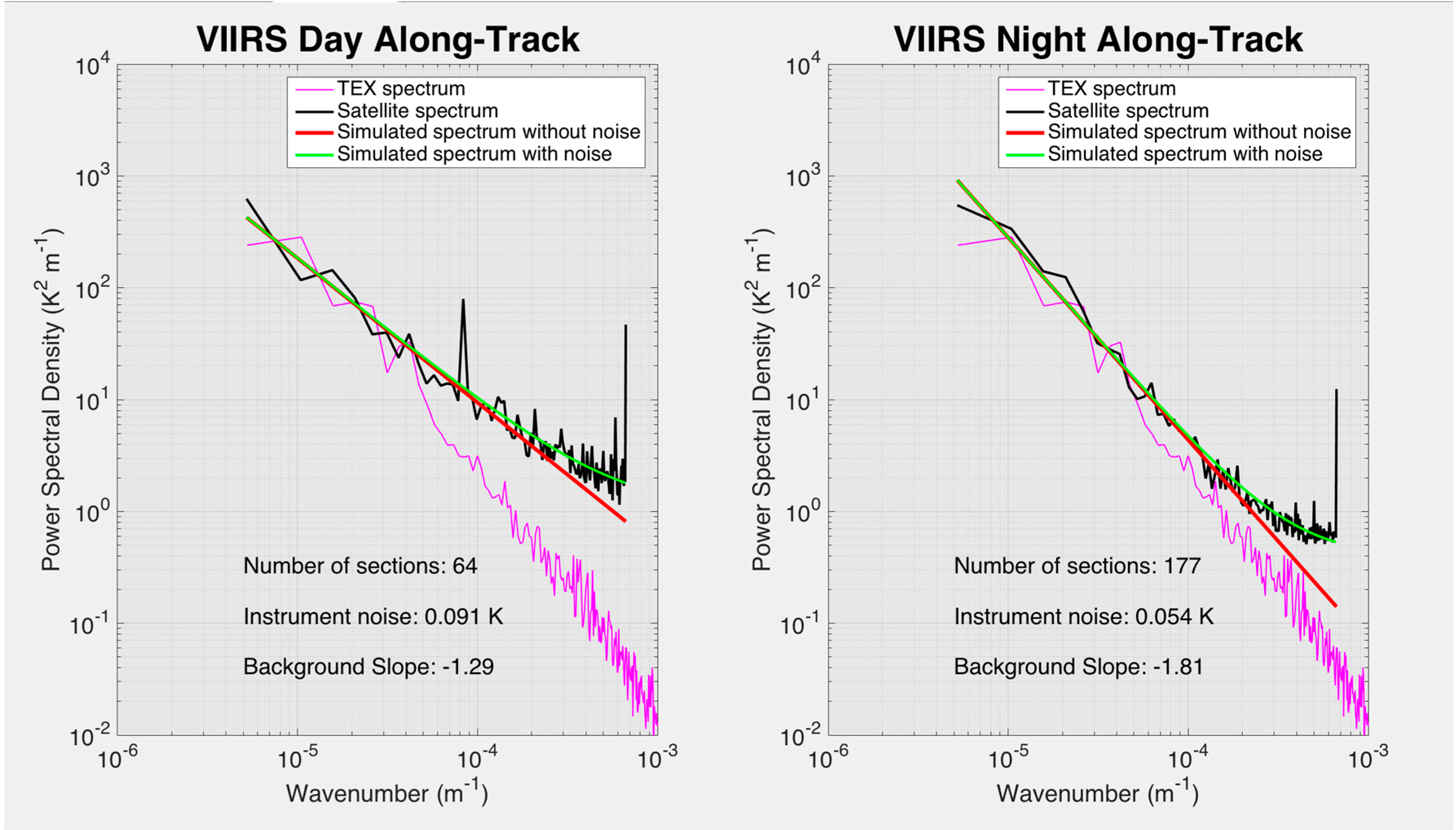
Mean VIIRS spectra similar to those shown for AVHRR in Figure 6 and Figure 7 are shown in Figure 8 and Figure 9, respectively. The spectra in these figures differ in several key ways from those associated with AVHRR. First, the level of instrument noise is, in all cases, substantially lower than that for AVHRR. Second, spectral peaks, especially in the daytime spectra, are evident at 1.5, 2.2, and 2.9 km as well as a broad peak at 12 km in the along-track spectra (Figure 9). There are 16 detectors for each of the VIIRS moderate resolution bands used for SST retrievals, hence, one scan of the instrument consists of 16 scan lines. The gain of these detectors may differ slightly and this difference is not regular, i.e., it changes along-scan and between scans. This is what gives rise to the observed peaks; the peaks at 1.5, 2.2, and 2.9 km correspond to a separation of one, two and three pixels and the peak at 12 km corresponds to the 16 pixel repeat scans of the instrument (750 m × 16 detectors = 12 km). Reassuringly, the along-scan spectra do not show these peaks. In addition, note that the noise from the different detectors contributes to a general elevation of the large wavenumber end of the spectrum—the simulated spectra with noise in Figure 9 tend to separate from the associated straight line spectrum at wavelengths smaller than approximately 8 km for along-track sections compared with approximately 5 km for along-scan sections. The point of separation is, of course, a function of the magnitude of the geophysical signal. In regions with a significantly larger geophysical signal, in the vicinity of the Gulf Stream for example, instrument noise will likely have no effect on the spectrum, with the possible exception of a few of the peaks.
The third significant difference between AVHRR and VIIRS spectra relates to the daytime spectra compared with the nighttime spectra. Specifically, there is a statistically significant difference between daytime and nighttime VIIRS spectra, with the daytime spectra being more energetic at wavelengths smaller than approximately 100 km. This is likely due to diurnal warming, which occurs frequently in the Sargasso Sea in summer months [14,18]. In addition, note that the slope of nighttime spectra for both along-scan and along-track sections is closer to that of the TEX spectrum than the daytime spectra. Surprisingly, the level of instrument noise is also larger at daytime than at nighttime as is evident both from the figures and from Table 3. This may result from the sensitivity of the banding to the energy in the SST field. Banding is difficult to correct for because it is not the entire scan line that has higher values than its neighbors, but rather, what appear to be randomly located segments of a given scan line. Furthermore, the magnitude of the difference in these regions appears to be related to the magnitude of the retrieved temperature.
Finally, the level of instrument noise estimated with the spectral approach is substantially smaller than (as much as one half) estimates based on the variogram. The reason for this is not clear. Although the spectral approach provides slightly better estimates of the noise added to simulated temperature sections than the approach based on the variogram, the estimates do not differ by the amounts seen in the actual data for VIIRS.
5. Discussion
5.1. Comparison of the AVHRR L2 Instrument Noise Estimates with the Results of Tandeo et al.
Tan14 estimated the nugget in the L3 Meteosat AVHRR data set produced by the O&SI SAF Project Team [6,22]. This product was assembled by remapping the full resolution nighttime AVHRR fields onto a regular 0.05° × 0.05° global grid and averaging the results into 12 h fields. They found for the study area. This is larger than would be expected if instrument noise of the full resolution Meteosat AVHRR data is similar to that found for NOAA-15 AVHRR (on the order of 0.20 K) and if this noise is uncorrelated from pixel-to-pixel, the assumption made in the analyses presented herein. Specifically, we would expect the noise for the L3 product to be approximately 0.05 K since order 25 pixels are averaged for each 0.05° × 0.05° SST estimate. It is possible that the level of instrument noise (elements in the yellow block of Figure 1) associated with the AVHRR on Meteosat is higher than that of NOAA-15. More likely however is that the difference results from misclassification errors associated with cloud flagging (the most significant element in the green block). Specifically, Tan14 processed all of the data for one year, 2008, i.e., they did not constrain their analysis to relatively cloud free fields as we did. Cloud-contaminated L2 pixels were, of course, excluded from the production of the L3 fields and Tan14 also excluded L3 pixels flagged as cloud-contaminated. However, the likelihood of misclassification, cloud-contaminated pixels not being flagged as such, increases as the fraction of cloud cover increases. Furthermore, classification errors tend to be small-scale errors, a small number of pixels here, a small number of pixels there, as opposed to large regions, which are misclassified. This means that such errors will likely contribute to noise at small spatial scales. A histogram of Tan14 nuggets (not shown here) shows a broad distribution ranging from in the 0.05 K range to order 0.3 K with a peak around 0.14 K. If the nugget resulted primarily from instrument errors (those in the yellow block), one would expect a relatively narrow peak; the instrument noise is unlikely to vary substantially for the region. Thus, the broad range suggests that it is a combination of classification errors and instrument noise. Because our analysis required long sections of cloud-free pixels the data were likely much more clear, on average, than those of Tan14. Noise may be added through the combination of L2 fields to obtain the L3 product, which also contributes to the difference between our estimate of local noise and that of Tan14. Using nighttime only data, as Tan14 have done, will minimize, but not completely remove, this. Finally, we found that the model, which best fits the SST field in the Sargasso Sea, varies from an exponential form to a Gaussian form, hence our use of the standard model. Tan14 used the exponential form. This will likely also contribute to an overestimate of the instrument noise in regions in which a mixed form is more appropriate.
Lending credence to the values we find, approximately 0.2 K for at both day and night, are the estimates of uncertainty found by Keogh et al. [23] when they compare AVHRR SST values with the values obtained from a ship-borne radiometer. They examined eight sections in eight images, five nighttime and three daytime. The SST values were close in space, most probably consisting of adjacent pixels and were obtained within three hours of the satellite pass. The resulting standard deviations thus represent a lower limit on the spatial precision of the AVHRR SST fields at that location (the English Channel). They obtained a standard deviation of the differences for each section. The average of these standard deviations is 0.22 K.
5.2. Impact of Noise on Sobel Gradient
Of interest is how levels of noise, typical of the values found thus far, impact gradients and fronts. In order to address this, we simulated 10,000 3 × 3 pixel squares for a given gradient in x, added Gaussian white noise to each of the elements, applied the 3 × 3 Sobel gradient operator in x and y to these squares and then determined the mean gradient and the standard deviation of the gradient. This was done for gradients ranging from 0.001 to 0.1 K km−1, values typical in the ocean, and for levels of instrument noise ranging from 0.01 K to 0.2 K. Figure 10 and Figure 11 show the means and standard deviations of the x- and y-components of the gradient, respectively. The mean x- and y-components are unaffected by the noise; the mean x-component is the same as the initial value and the mean y-component is very nearly zero. The standard deviation of the components is very nearly independent of the imposed noise. For a noise level typical of VIIRS, 0.05 K, the vertical white lines in the figures, the uncertainty of each of the components is approximately 0.022 K and for a level typical of AVHRR, 0.2 K, the uncertainty in the components is 0.09 K. In general, the uncertainty in the given component is approximately one half of the level of imposed noise.
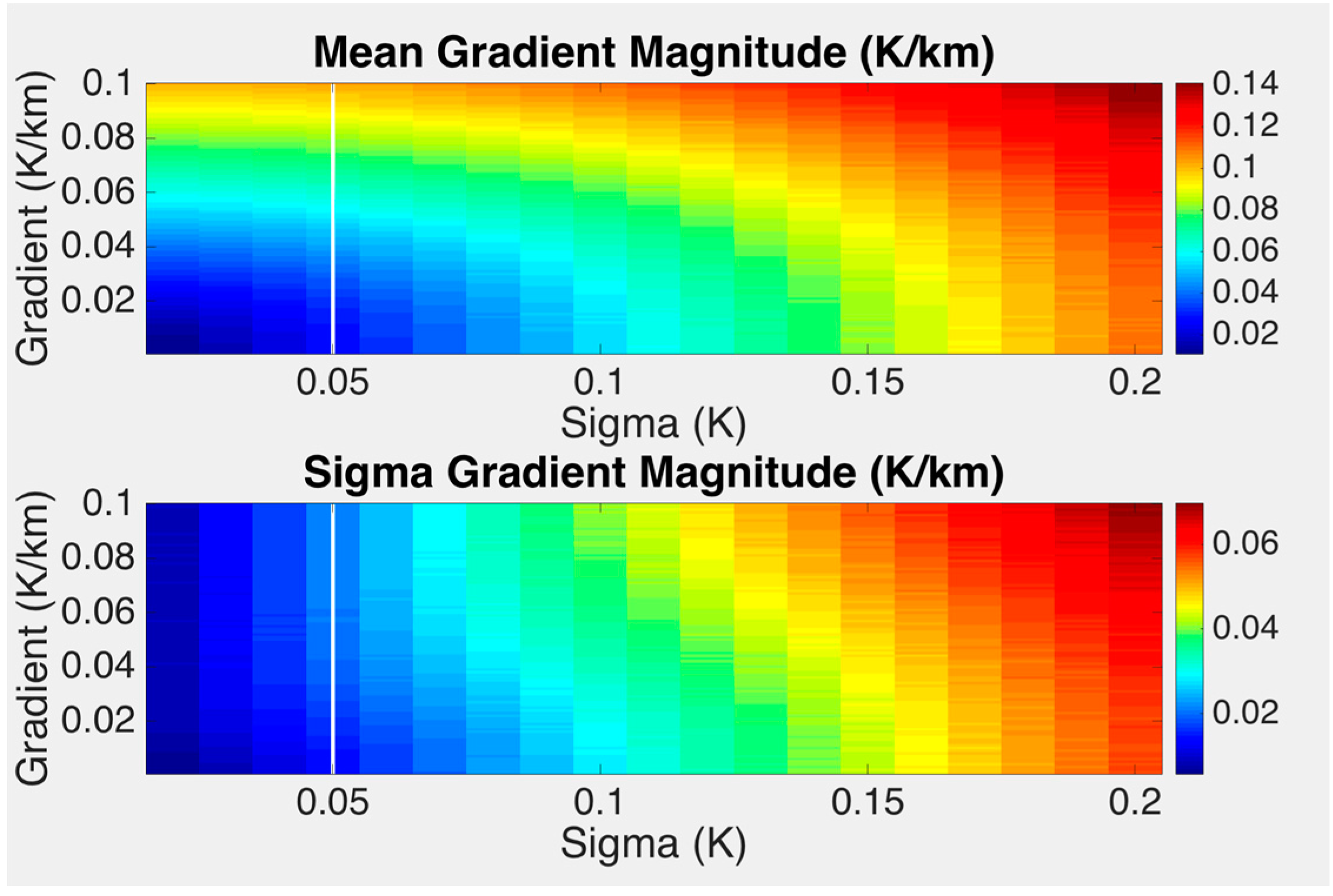
The impact on the gradient magnitude (Figure 12) is more dramatic. The mean of the estimated gradient is no longer equal to the magnitude of the imposed gradient. For example, for a relatively robust gradient of 0.05 K/km, the mean of the estimated gradient ranges from 0.05 to in excess of 0.1 K/km as the imposed noise increases from 0 to 0.2 K/km. Note that contours of the estimated gradient tend to become level for imposed noise levels less than approximately 0.07 K. This means that VIIRS estimates of the mean gradient magnitude will be centered on the actual value of the gradient, but that the gradient magnitude will be substantially overestimated in AVHRR fields. The uncertainty of the estimated gradient magnitude increases with the imposed noise, nearly doubling from the value associated with a zero imposed gradient to an imposed gradient of 0.1 K/km. These observations do not mean that a front with a gradient of this magnitude (0.05 K/km) is undetectable in a field with an AVHRR noise level but detection will be problematic. Simulations using front detection algorithms need to be undertaken to evaluate this. Although none of this is surprising, we are not aware of any studies involving the gradient magnitude of satellite-derived SST fields accounting for this—including many of our own.
6. Conclusions
The accuracy with which the local gradient of any digital field can be determined is a function of the spatial precision of the underlying data, where the spatial precision is defined as the square root of the variance of individual pixel values following removal of real trends in the data and removal of noise that is correlated over scales that are large compared with the scale used to calculate the gradient. In the case of fields obtained from satellite-borne sensors, this noise is attributed to characteristics of the sensor, “instrument noise”, and to the retrieval process, “retrieval noise”. Two approaches, a spectral-based approach and a variogram-based approach, were used to estimate the instrument portion of this noise in L2 AVHRR and VIIRS SST fields. To reduce the non-instrument portion of the local noise in the analysis, only cloud free sections were used, the assumption being that the dominant contribution to the non-instrument local noise is due to the misclassification of clouds. Because instrument noise was thought to differ between the along-scan and along-track directions and because the geophysical variance was thought to differ between day and night, the analysis was performed separately for the four along-scan/along-track and day/night combinations.
Both methods yielded similar results for AVHRR, with daytime and nighttime along-scan values of ~0.18 K and along-track values of 0.21 K. VIIRS instrument noise, on the other hand, was found to differ by method, scan geometry and day-versus-night–ranging from 0.021 K for the nighttime, along-scan spectral estimate to 0.097 K for the daytime, along-track variogram estimate. Day and night along-scan estimates based on the spectral approach are close to one half those based on the variogram. For both methods, the nighttime estimates are also roughly one half the corresponding daytime estimates. Finally, the along-track estimates are roughly 50% larger than the along-scan estimates for the spectral approach but only about 25% larger when based on the variogram. In all cases, the estimates were smaller than the “upper limit”.
In summary, VIIRS instrument noise is substantially smaller than AVHRR instrument noise, with levels as low as 0.02 K in the along-scan direction at nighttime. In fact, VIIRS instrument noise under these conditions is near the level of the geophysical signal in the dynamically quietest regions in the ocean.
Acknowledgments
This research was supported by the Global Change Research Program of China (2015CB953901), the National Natural Science Foundation of China-Shandong Joint Fund for Marine Science Research Centers (U1606405), the National Natural Science Foundation of China (41376105, 41574014, 41774014), the Scientific and Technological Innovation Project of Qingdao National Laboratory for Marine Science and Technology (2016ASKJ16), the National Oceanographic and Atmospheric Administration (NA11NOS0120167), the National Aeronautics and Space Administration (NNX16AI24G) and the Frontier science and technology innovation project of the Science and Technology Commission of the Central Military Commission (085015). Salary support for F.W. was provided by the China Scholarship Council and Ocean University of China. Salary support for P.C. was provided by the state of Rhode Island and Providence Plantations.
Author Contributions
Fan Wu and Peter Cornillon conceived, designed and performed the experiments, and wrote the paper; Brahim Boussidi performed the experiments of variogram approach; and Lei Guan provided suggestion to the experiments and the analysis of the results.
Conflicts of Interest
The authors declare no conflict of interest.
Acronyms
| AVHRR | Advanced Very High Resolution Radiometer |
| DFT | Discrete Fourier Transform |
| FFT | Fast Fourier Transform |
| GHRSST | Group on High Resolution Sea Surface Temperature |
| HRPT | High Resolution Picture Transmission |
| JPSS | Joint Polar Satellite System |
| NPP | National Polar-orbiting Partnership |
| PSD | Power Spectral Density |
| SST | Sea Surface Temperature |
| VIIRS | Visible-Infrared Imager-Radiometer Suite |
References and Notes
- Strong, A.E.; McClain, E.P. Improved ocean surface temperatures from space-comparisons with drifting buoys. Bull. Am. Meteorol. Soc. 1984, 65, 138–139. [Google Scholar] [CrossRef]
- Guo, P.; Bo, Y. Validation of AVHRR/MODIS/AMSR-E satellite SST products in the west tropical Pacific. In Proceedings of the 2008 IEEE International Geoscience and Remote Sensing Symposium (IGARSS), Boston, MA, USA, 6–11 July 2008; Volume 4, pp. 942–945. [Google Scholar]
- Park, K.A.; Lee, E.Y.; Li, X.; Chung, S.R.; Sohn, E.H.; Hong, S. NOAA/AVHRR sea surface temperature accuracy in the East/Japan Sea. Int. J. Digit. Earth 2015, 8, 784–804. [Google Scholar] [CrossRef]
- Petrenko, B.; Ignatov, A.; Stroup, J.; Dash, P. Evaluation and Selection of SST Regression Algorithms for JPSS VIIRS. J. Geophys. Res. Atmos. 2014, 119, 4580–4599. [Google Scholar] [CrossRef]
- Tu, Q.; Pan, D.; Hao, Z. Validation of S-NPP VIIRS sea surface temperature retrieved from NAVO. J. Remote Sens. 2015, 7, 17234–17245. [Google Scholar] [CrossRef]
- Tandeo, P.; Autret, E.; Chapron, B.; Fablet, R.; Garello, R. SST spatial anisotropic covariances from METOP-AVHRR data. J. Remote Sens. Environ. 2014, 141, 144–148. [Google Scholar] [CrossRef] [Green Version]
- Donlon, C.; Rayner, N.; Robinson, I.; Poulter, D.J.S.; Casey, K.S.; Vazquez-Cuervo, J.; Armstrong, E.; Bingham, A.; Arino, O.; Gentemann, C.; et al. The Global Ocean Data Assimilation Experiment High-resolution Sea Surface Temperature Pilot Project. Bull. Am. Meteorol. Soc. 2007, 88, 1197–1213. [Google Scholar] [CrossRef]
- “Level-2” Refers to the Processing Level of the Data, a Nomenclature Used Extensively for Satellite-Derived Datasets, Although the Precise Meaning of the Level of Processing Varies by Organization. The Definition Promulgated by the Group on High Resolution Sea Surface Temperature (GHRSST) Is Used Here. Available online: http://science.nasa.gov/earth-science/earth-science-data/data-processing-levels-for-eosdis -data-products/ (accessed on 21 August 2017).
- Cornillon, P.; Castro, S.; Gentemann, C.; Jessup, A.; Kaplan, A.; Lindstrom, E.; Maturi, E.; Minnett, P.J.; Reynolds, R. SST Error Budget—White Paper. 2010. Available online: https://works.bepress.com/peter-cornillon/1/ (accessed on 21 August 2017).
- Schloesser, F.; Cornillon, P.C.; Donohue, K.; Boussidi, B.; Iskin, E. Evaluation of thermosalinograph and VIIRS data for the characterization of near-surface temperature fields. J. Atmos. Ocean. Technol. 2016, 33, 1843–1858. [Google Scholar] [CrossRef]
- Seaman, C.; Hillger, D.; Kopp, T.; Williams, R.; Miller, S.; Lindsey, D. Visible Infrared Imaging Radiometer Suite (VIIRS) Imagery Environmental Data Record (EDR) User’s Guide. Version 1.1. Available online: http://rammb.cira.colostate.edu/projects/npp/VIIRS_Imagery_EDR_Users_Guide.pdf (accessed on 21 August 2017).
- Schueler, C.F.; Clement, J.E.; Ardanuy, P.E.; Welsch, C.; DeLuccia, F.; Swenson, H. NPOESS VIIRS sensor design overview. Proc. SPIE 2002, 4483, 11–23. [Google Scholar]
- Kilpatrick, K.A.; Podestá, G.P.; Evans, R. Overview of the NOAA/NASA advanced very high resolution radiometer Pathfinder algorithm for sea surface temperature and associated matchup database. J. Geophys. Res. Oceans 2001, 106, 9179–9198. [Google Scholar] [CrossRef]
- Stramma, L.; Cornillon, P.C.; Weller, R.A.; Price, J.F.; Briscoe, M.G. Large Diurnal sea surface temperature variability: Satellite and in situ measurements. J. Phys. Oceanogr. 1986, 16, 827–837. [Google Scholar] [CrossRef]
- Wang, D.P.; Flagg, C.N.; Donohue, K.; Rossby, H.T. Wavenumber spectrum in the Gulf Stream from shipboard ADCP observations and comparison with altimetry measurements. J. Phys. Oceanogr. 2010, 40, 840–844. [Google Scholar] [CrossRef]
- Cayula, J.F.P.; Cornillon, P.C. Edge detection algorithm for SST images. J. Atmos. Ocean. Technol. 1992, 9, 67–80. [Google Scholar] [CrossRef]
- Bouali, M.; Ignatov, A. Adaptive reduction of striping for improved sea surface temperature imagery from Suomi National Polar-Orbiting Partnership (S-NPP) Visible Infrared Imaging Radiometer Suite (VIIRS). J. Atmos. Ocean. Technol. 2013, 31, 150–163. [Google Scholar] [CrossRef]
- Cornillon, P.C.; Stramma, L. The distribution of diurnal sea surface warming events in the western Sargasso Sea. J. Geophys. Res. Oceans 1985, 90, 11811–11815. [Google Scholar] [CrossRef]
- Barnes, S.L. A technique for maximizing details in numerical weather map analysis. J. Appl. Meteorol. 1964, 3, 396–409. [Google Scholar] [CrossRef]
- Wackernagel, H. Multivariate Geostatistics: An Introduction with Applications; Springer Science & Business Media, Inc.: New York, NY, USA, 2013. [Google Scholar]
- Cressie, N.A.C. Statistics for Spatial Data; (Revised Edition); John Wiley and Sons, Inc.: New York, NY, USA, 1993. [Google Scholar]
- O&SI SAF Project Team. Low Earth Orbiter Sea Surface Temperature Product User Manual. Available online: http://www.osi-saf.org (accessed on 21 August 2017).
- Keogh, S.J.; Robinson, I.S.; Donlon, C.J.; Nightingale, T.J. The accuracy of AVHRR SST determined using shipborne radiometers. J. Remote Sens. 1999, 20, 2871–2876. [Google Scholar] [CrossRef]
Figure 1.
The error budget developed by the National Aeronautics and Space Administration (NASA)-National Oceanic and Atmospheric Administration (NOAA) sea surface temperature (SST) Science Team for satellite-derived SST fields.
Figure 1.
The error budget developed by the National Aeronautics and Space Administration (NASA)-National Oceanic and Atmospheric Administration (NOAA) sea surface temperature (SST) Science Team for satellite-derived SST fields.
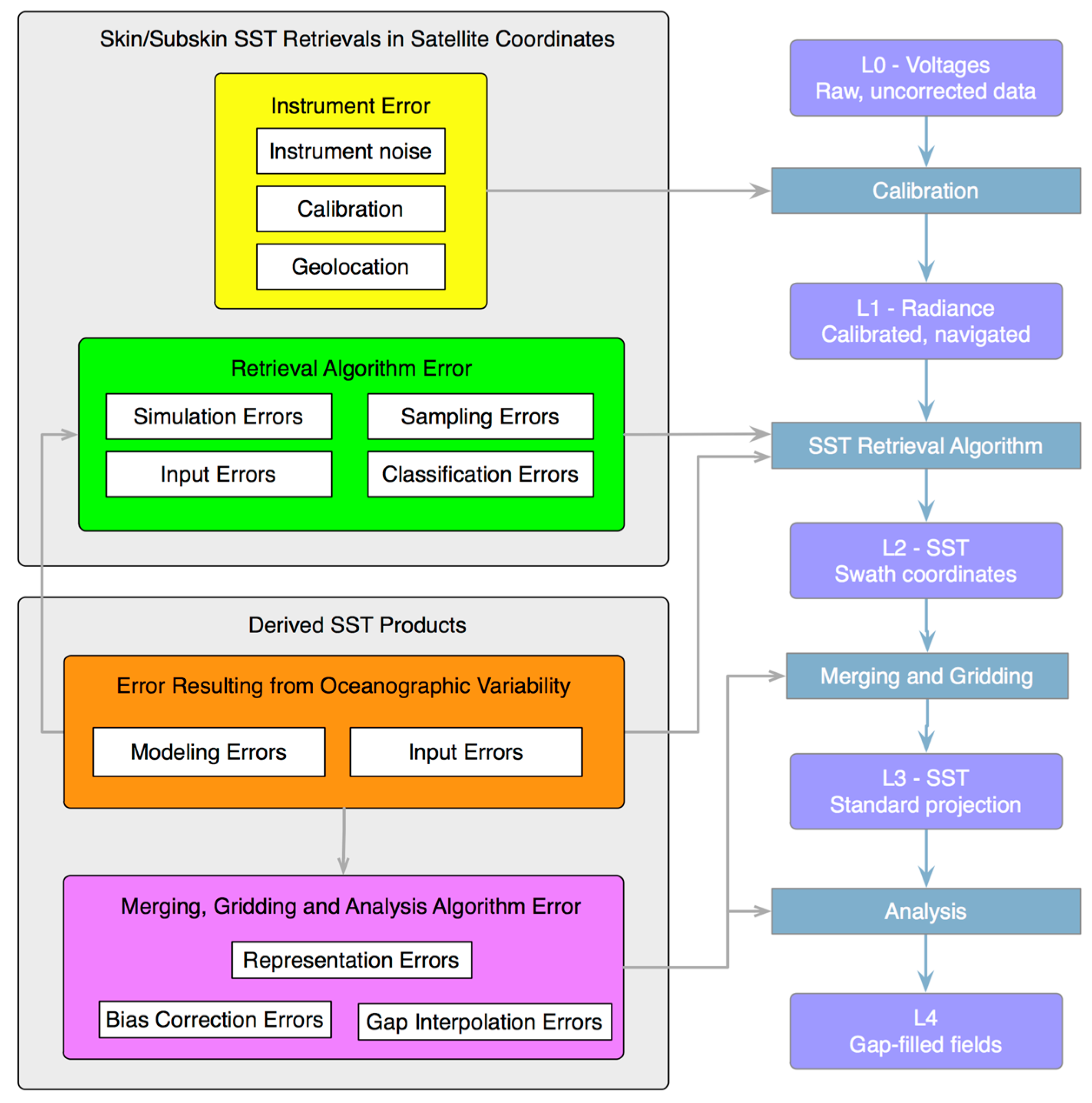
Figure 2.
Visible-Infrared Imager-Radiometer Suite (VIIRS) SST image from 12 May 2012. The long black line (73.5°W, 40°N to 64.8°W, 32.6°N) indicates the nominal Oleander track. Blue frame (longitudes from 63°W to 72°W, and latitudes from 32°N to 36°N) denotes the region of the Sargasso Sea considered in this study. Shades of gray denote the location of sections extracted from VIIRS SST fields—discussed in Section 3.1.1. The gray scale indicates distance from nadir (discussed in detail in subsequent sections). Sections with a constant gray level are along-track sections; those with a gradient in gray are along-scan. Along-track (along-scan) sections with a negative slope and along-scan (along-track) sections with a positive slope are daytime (nighttime) sections. The SST field is simply provided as a background reference field and corresponds to only one of the images used.
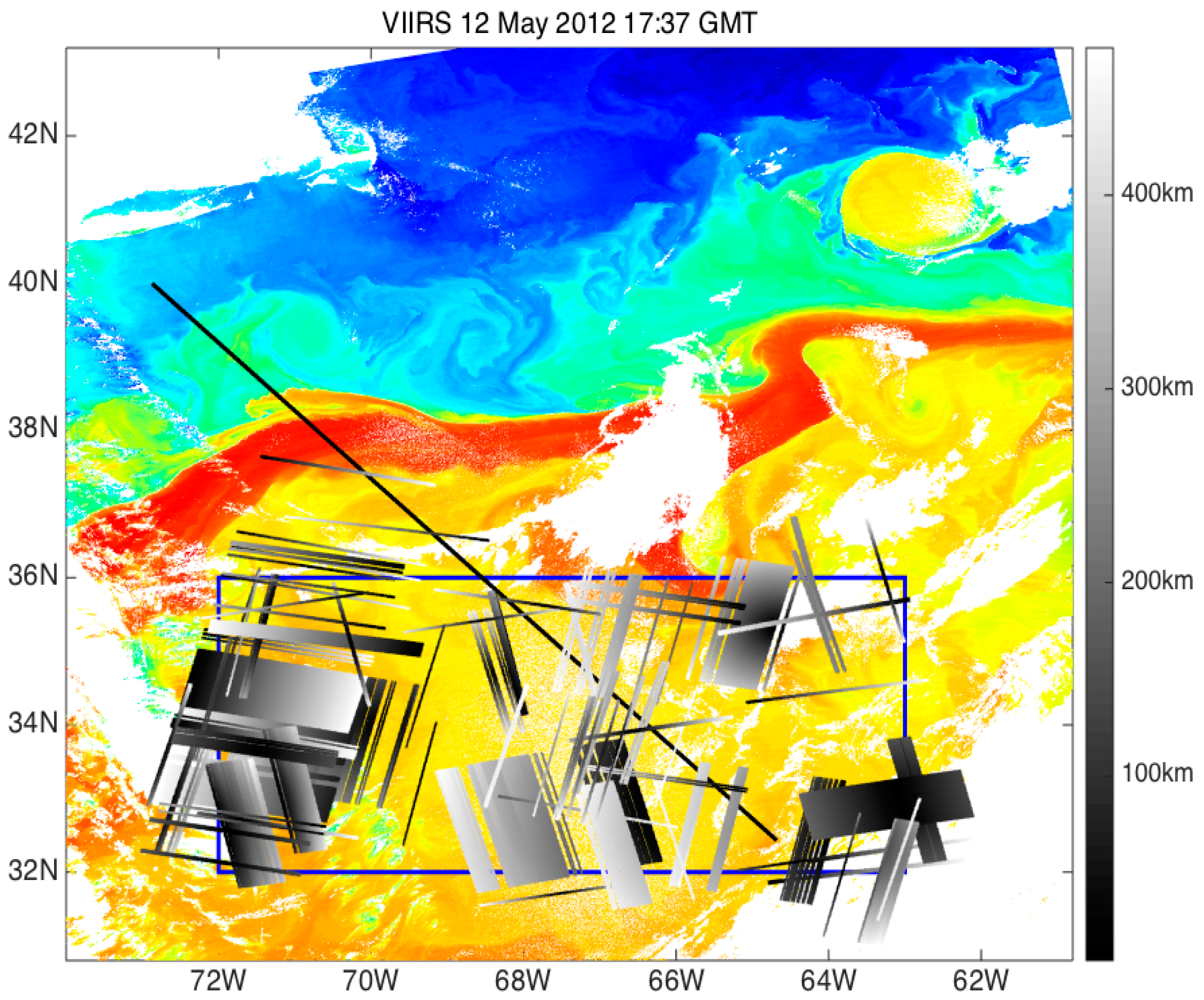
Figure 3.
Spacing in the along-scan direction for Advanced Very High Resolution Radiometer (AVHRR) and VIIRS pixels in L2 fields as a function of distance from nadir.
Figure 3.
Spacing in the along-scan direction for Advanced Very High Resolution Radiometer (AVHRR) and VIIRS pixels in L2 fields as a function of distance from nadir.

Figure 4.
Spectral response of the interpolation methods applied to white noise.
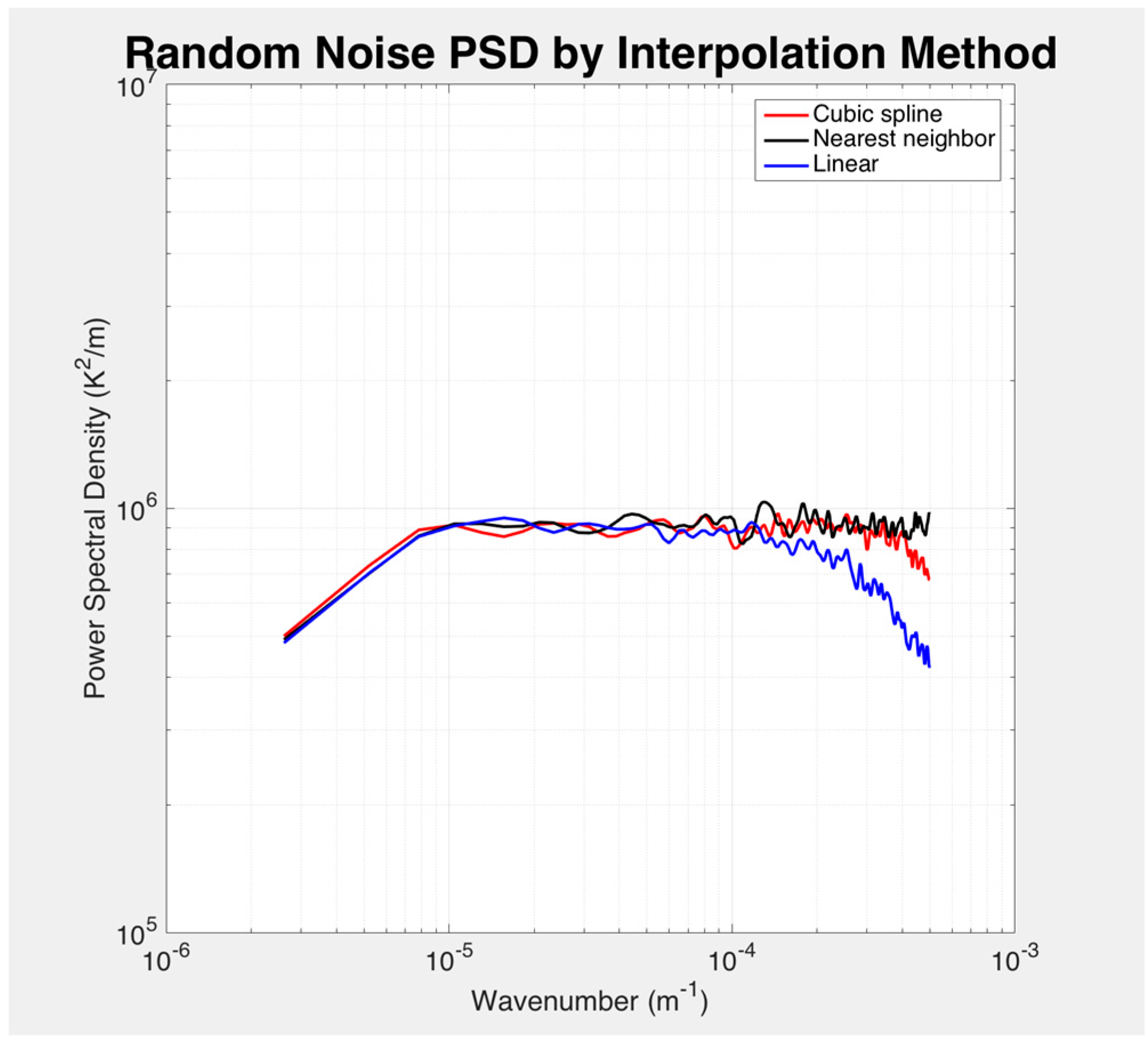
Figure 5.
Power spectral density from Oleander TEX for all Oleander summer sections (June–August) of 2008 through 2013 with maximum sample separation less than 150 m. Temperature sections detrended prior to determining and ensemble averaging the spectra. Straight red line: least squares best fit straight line (slope = −2.12) of log10 (PSD) to log10 (wavenumber) between 10−5 and 10−3 m−1.

Figure 6.
Mean AVHRR spectra for contiguous along-scan sections (black). Best-fit linear spectra with noise to the mean VIIRS spectra (green). Best-fit linear portion of the best-fit linear spectra with noise (red). Mean TEX spectrum shifted vertically to allow for comparison (magenta).
Figure 6.
Mean AVHRR spectra for contiguous along-scan sections (black). Best-fit linear spectra with noise to the mean VIIRS spectra (green). Best-fit linear portion of the best-fit linear spectra with noise (red). Mean TEX spectrum shifted vertically to allow for comparison (magenta).

Figure 7.
Mean AVHRR spectra similar to Figure 6 except for along-track sections. Daytime spectrum is for 21:08 GMT on 10 June 2012. Nighttime spectrum is for 09:34 GMT on 23 June 2012.
Figure 7.
Mean AVHRR spectra similar to Figure 6 except for along-track sections. Daytime spectrum is for 21:08 GMT on 10 June 2012. Nighttime spectrum is for 09:34 GMT on 23 June 2012.

Figure 8.
Mean VIIRS spectra similar to the AVHRR spectra in Figure 6.
Figure 8.
Mean VIIRS spectra similar to the AVHRR spectra in Figure 6.
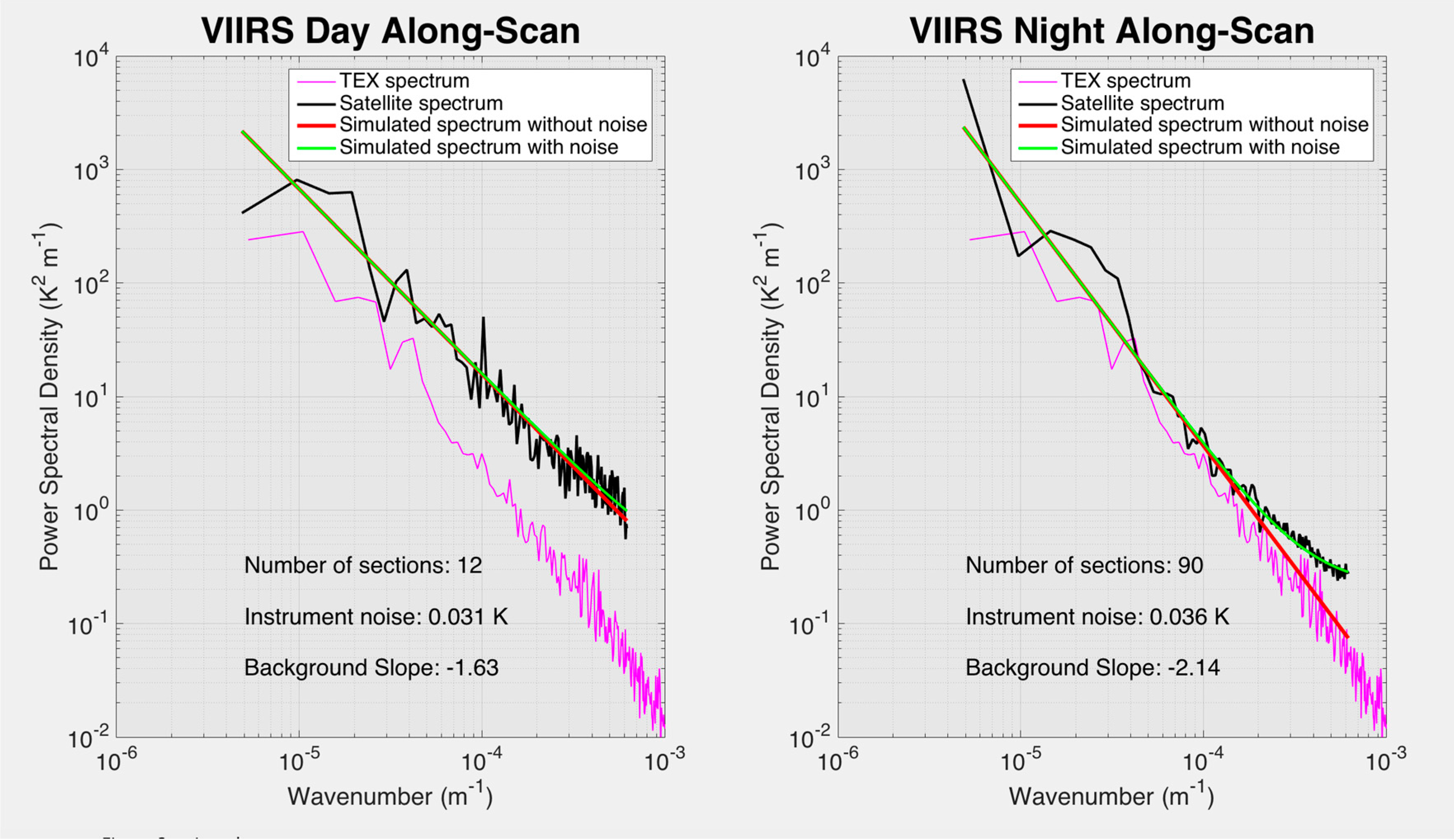
Figure 9.
Mean VIIRS spectra similar to the AVHRR spectra in Figure 7.
Figure 9.
Mean VIIRS spectra similar to the AVHRR spectra in Figure 7.

Figure 10.
Simulated impact of Gaussian white noise of magnitude sigma imposed on a field with an x-gradient indicated on the vertical axis. The vertical white line is an imposed noise level typical of VIIRS values.
Figure 10.
Simulated impact of Gaussian white noise of magnitude sigma imposed on a field with an x-gradient indicated on the vertical axis. The vertical white line is an imposed noise level typical of VIIRS values.
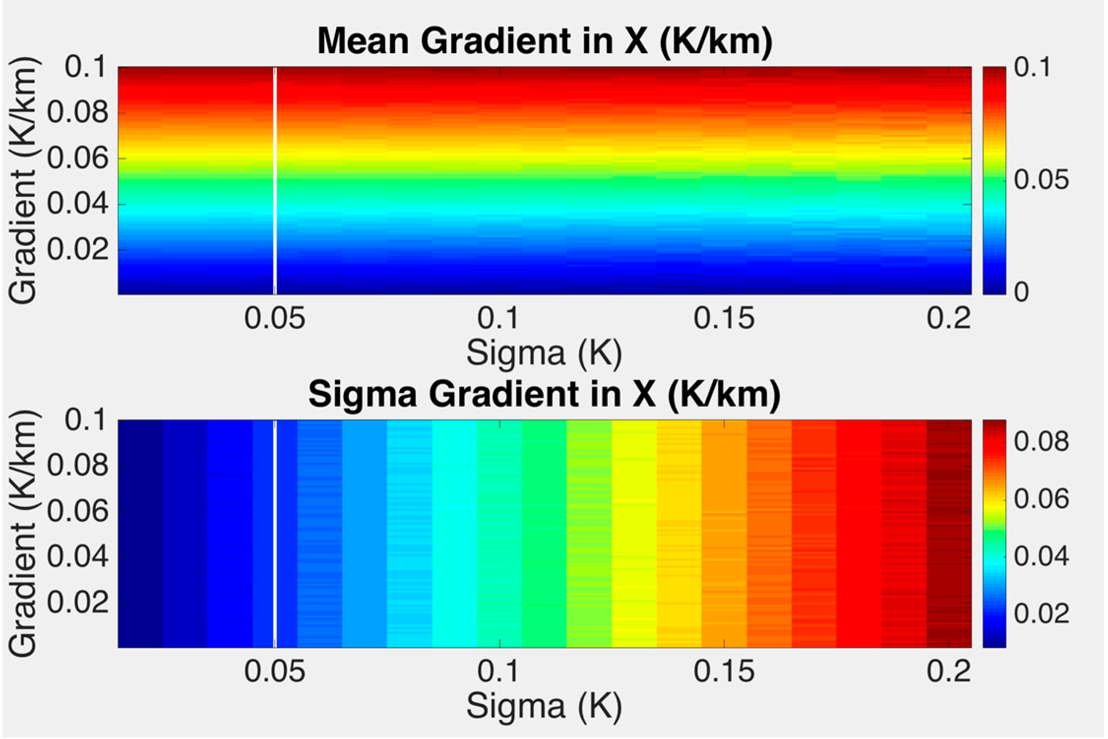
Figure 11.
As in Figure 10 except for the y-component of the gradient.
Figure 11.
As in Figure 10 except for the y-component of the gradient.
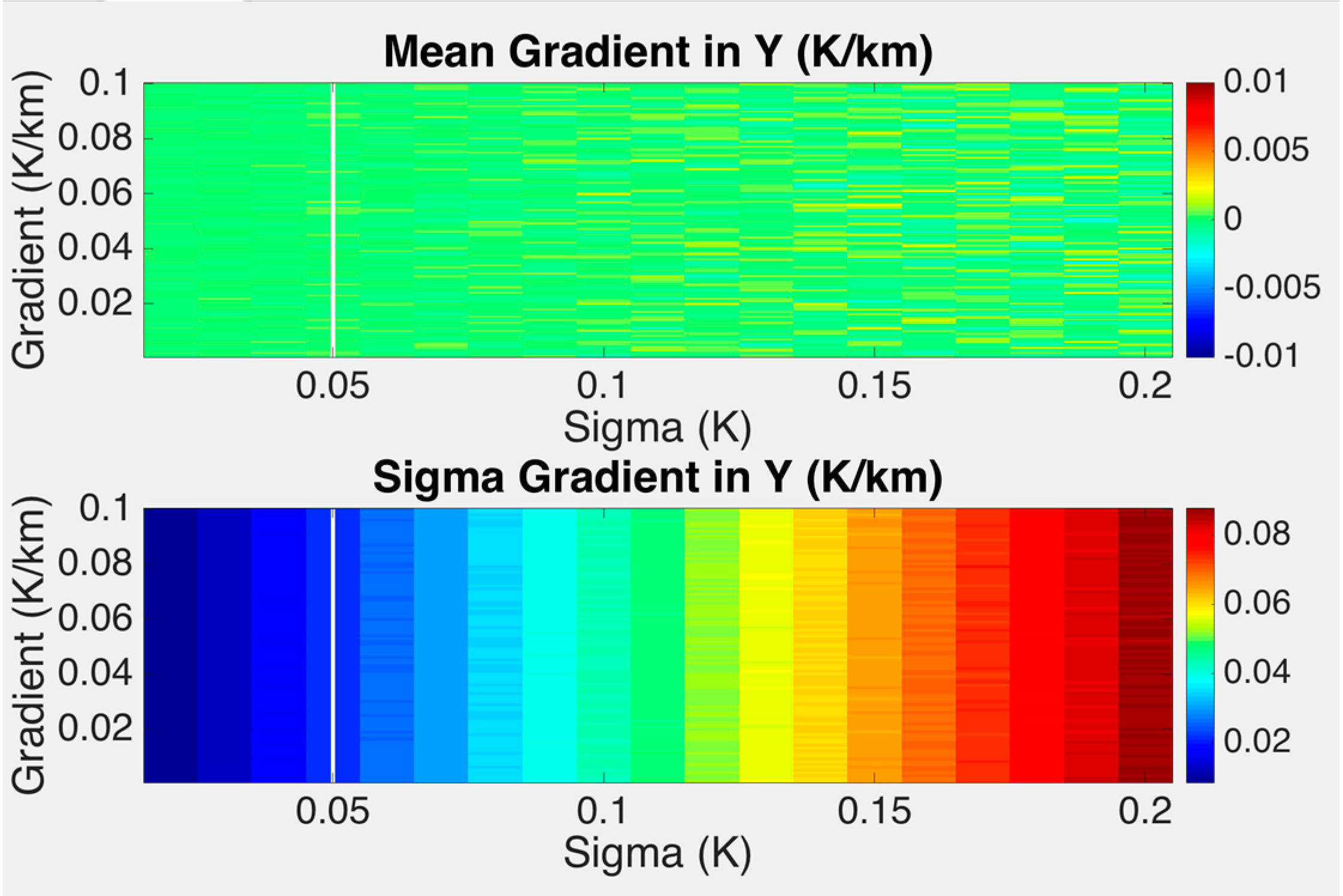
Figure 12.
As for Figure 10 except for the gradient magnitude.
Figure 12.
As for Figure 10 except for the gradient magnitude.


Table 1.
Number of sections meeting the given selection criteria discussed in this section and in Section 2.4 and Section 2.5.
Table 1.
Number of sections meeting the given selection criteria discussed in this section and in Section 2.4 and Section 2.5.
| Day | Night | |||
|---|---|---|---|---|
| Along-Scan | Along-Track | Along-Scan | Along-Track | |
| VIIRS | 126 | 517 | 561 | 615 |
| AVHRR | 266 | 256 | 104 | 193 |
| Oleander | 42 | |||
Table 2.
Grouping of along-scan sections based on mean pixel spacing of the temperature section. The values indicated correspond to the lower limit on the range—the value to which temperature sections in the range is interpolated—the upper limit on the range.
Table 2.
Grouping of along-scan sections based on mean pixel spacing of the temperature section. The values indicated correspond to the lower limit on the range—the value to which temperature sections in the range is interpolated—the upper limit on the range.
| Group 1 (m) | Group 2 (m) | Group 3 (m) | |
|---|---|---|---|
| VIIRS | 770-805-820 | 860-885-910 | 940-995-980 |
| AVHRR | 760-765-810 | 820-865-920 | 940-947-980 |
Table 3.
Estimated instrument noise in satellite-derived SST fields. Numbers in parentheses are the number of subgroups from which the means are determined. The indicated uncertainty of the means is the square root of the variance of the contributing subgroups over the number of subgroups.
Table 3.
Estimated instrument noise in satellite-derived SST fields. Numbers in parentheses are the number of subgroups from which the means are determined. The indicated uncertainty of the means is the square root of the variance of the contributing subgroups over the number of subgroups.
| Method | Day (K) | Night (K) | |||
|---|---|---|---|---|---|
| Along-Scan | Along-Track | Along-Scan | Along-Track | ||
| AVHRR | Spectra | 0.172 ± 0.001 (5) | 0.209 ± 0.001 (7) | 0.173 ± 0.003 (2) | 0.209 ± 0.008 (4) |
| Variogram | 0.185 ± 0.004 (5) | 0.219 ± 0.006 (7) | 0.183 ± 0.001 (2) | 0.219 ± 0.006 (4) | |
| Upper Limit | 0.189 | 0.218 | 0.194 | 0.208 | |
| VIIRS | Spectra | 0.046 ± 0.001 (4) | 0.076 ± 0.002 (10) | 0.021 ± 0.001 (24) | 0.032 ± 0.002 (14) |
| Variogram | 0.081 ± 0.013 (4) | 0.097 ± 0.006 (10) | 0.042 ± 0.004 (24) | 0.056 ± 0.004 (13) | |
| Upper Limit | 0.078 | 0.101 | 0.050 | 0.057 | |
© 2017 by the authors. Licensee MDPI, Basel, Switzerland. This article is an open access article distributed under the terms and conditions of the Creative Commons Attribution (CC BY) license (http://creativecommons.org/licenses/by/4.0/).
Share and Cite
MDPI and ACS Style
Wu, F.; Cornillon, P.; Boussidi, B.; Guan, L. Determining the Pixel-to-Pixel Uncertainty in Satellite-Derived SST Fields. Remote Sens. 2017, 9, 877. https://doi.org/10.3390/rs9090877
AMA Style
Wu F, Cornillon P, Boussidi B, Guan L. Determining the Pixel-to-Pixel Uncertainty in Satellite-Derived SST Fields. Remote Sensing. 2017; 9(9):877. https://doi.org/10.3390/rs9090877
Chicago/Turabian StyleWu, Fan, Peter Cornillon, Brahim Boussidi, and Lei Guan. 2017. "Determining the Pixel-to-Pixel Uncertainty in Satellite-Derived SST Fields" Remote Sensing 9, no. 9: 877. https://doi.org/10.3390/rs9090877
Note that from the first issue of 2016, this journal uses article numbers instead of page numbers. See further details here.