
Technical Evaluation of Sentinel-1 IW Mode Cross-Pol Radar Backscattering from the Ocean Surface in Moderate Wind Condition


1
Shanghai Key Laboratory of Intelligent Sensing and Recognition, Shanghai Jiao Tong University, Shanghai 200240, China
2
Global Science and Technology, National Oceanic and Atmospheric Administration (NOAA)/NOAA Satellite and Information Service, College Park, MD 20740, USA
*
Author to whom correspondence should be addressed.
Remote Sens. 2017, 9(8), 854; https://doi.org/10.3390/rs9080854
Submission received: 30 June 2017
/
Revised: 5 August 2017
/
Accepted: 16 August 2017
/
Published: 17 August 2017
(This article belongs to the Special Issue Ocean Remote Sensing with Synthetic Aperture Radar)
Abstract
:The Sentinel-1 synthetic aperture radar (SAR) allows sufficient resources for cross-pol wind speed retrievals over the ocean. In this paper, we present technical evaluation on wind retrieval from both Sentinel-1A and Sentinel-1B IW cross-pol images. Algorithms are based on the existing theoretical and empirical ones derived from the RADARSAT-2 cross-pol data. First, to better understand the Sentinel-1 observed normalized radar cross section (NRCS) values under various environmental conditions, we constructed a dataset that integrates SAR images with wind field information from scatterometer measurements. There are 11,883 matchup data in the experimental dataset. We then calculated the systemic noise floor of Sentinel-1 IW mode, and presented its unique noise characteristics among different sub-bands. Based on the calculated NESZ measurements, the noise is removed for all matchup data. Empirical relationships among the noise free NRCS , wind speed, wind direction, and radar incidence angle are analyzed for each sub-band, and a piecewise model is proposed. We showed that a larger correlation coefficient, r, is achieved by including both wind direction and incidence terms in the model. Validation against scatterometer measurements showed the suitability of the proposed model.
1. Introduction
Synthetic aperture radar (SAR) images provide deep knowledge of the characteristics of wind fields over both the ocean and littoral zones with high spatial resolution. Due to the complex electromagnetic scattering mechanism of SAR, empirical approaches of wind field retrievals based on geophysical model functions (GMF), which describe the dependence of the normalized radar cross section (NRCS) with respect to wind vectors and incidence angles, are widely investigated. For C-band co-polarization (co-pol) SAR images, along with a polarization ratio model for HH polarizations, many GMF models are developed [1,2,3,4,5,6]. However, the NRCS of co-pol exhibits data saturated when wind speed exceeds about 16 for incidence angle under [7]. Otherwise, the cross-polarization (cross-pol) shows that the signal increases with wind speed and does not saturate even at very high speeds. Therefore, cross-pol data has been widely used for high wind speed retrievals [7,8,9,10,11].
Some related assessments and evaluations of cross-pol images have been done to RADARSAT-2 quad polarization (quad-pol) which have lower noise (about ). By collocating quad-pol RADARSAT-2 SAR images and buoy measurements, Vachon and Wolfe in 2011 have shown that the cross-pol backscattering is independent of incidence angle and wind direction, and developed a monotonic linear relationship between cross-pol backscattering and wind speed [12]. In [7], Hwang et al. have shown that the linearly increasing relationship between the NRCS in moderate wind conditions (about <) gradually transits to cubic in high wind conditions (about >). Bergeron et al. [13] compared the wind retrieval performances of two models proposed by Vachon [12] and Hwang [7] for wind speed retrieval in cross-pol. These researches describe the relationship between the NRCS and wind speeds assuming that cross-pol is independent on the variations of incidence angles. In [14], the incidence angle and wind direction dependences of cross-pol radar backscattering are analyzed and theoretically explained.
Some researches concentrated on wind retrieval using C-band high noise data in dual polarization (dual-pol) such as RADARSAT-2 ScanSAR mode, Sentinel-1 and planned RADARSAT Constellation. Differ from RADARSAT-2 quad-pol data which have lower noise (about ), the wide swath RADARSAT-2 ScanSAR have higher noise (about ) [14]. In [15], Shen et al. indicate that dual-pol and quad-pol exhibit different relationships with wind speed, therefore a distinct model particularly for high noise dual-pol data wind retrieval is required. For RADARSAT-2 ScanSAR mode images, existing wind retrieval models only consider wind speed dependence [15,16]. In [16], the NRCS is found to be a linear function of wind speed, thus the C-2POD model was derived for hurricane wind retrieval. A two-piecewise linear GMF model was developed to quantify the relationship between the NRCS and wind speeds [15]. In [17], the wind direction dependence of NRCS is analyzed. Zhang et al. [11] proposed a hybrid backscattering model to carry out theoretically analyze the relationship among both VH and VV polarized NRCS, wind speed and incidence angle. Using this hybrid model, a hurricane wind retrieval model named C-3PO was developed, by including dependence on incidence angle.
With the free and open data policy of Sentinel-1 satellites, VH dual polarization SAR images have become publicly available, allowing sufficient resources for cross-pol wind speed retrievals. In [18], based on Sentinel-1 VV polarization images, the spatial characteristics of the SAR-derived winds are presented, and the detailed descriptions of the wind fields provided by SAR are analyzed. Monaldo et al. [19] evaluate the performance of Sentinel-1A wind speed retrievals using GMFs (CMOD4, CMOD_IF2, CMOD5,CMOD5.N), and conclude good agreement of Advanced SCATterometer (ASCAT) wind speeds and Sentinel-1 VV and HH measurements. However, for Sentinel-1 cross-pol SAR images, their radar backscattering from the ocean surface and technical performance for wind speed retrievals are yet to be evaluated.
The planned RADARSAT Constellation Mission (RCM), which will be launched in 2018, is designed primarily to be dedicated to regular monitoring with various modes and resolutions [20]. Among the main operational modes, the Medium Resolution 50 m mode was designed for general-purpose wide area surveillance [21,22]. It is 4 looks and a imaging swath, and is comparable to the RADARSAT-2 ScanSAR mode, thus it is promising to be employed in marine wind application [21,22]. We expect that there will be more available C-band high noise data such as Sentinel-1 and RCM in the coming years. Therefore, wind retrieval model designed for C-band high noise data is required.
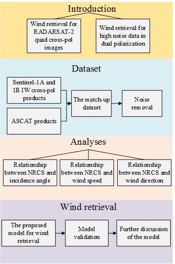
In this paper, with the rapidly growing availability of Sentinel-1 data, we revisit the empirical relationships between cross-pol radar backscattering and wind speeds with attention to evaluate contribution from incidence angle and wind direction terms. A model for moderate wind speed retrieval is proposed, by including the dependences on wind speed, incidence angle, and wind direction. The scopes of this paper are to give a technical evaluation of Sentinel-1 cross-pol images based on the theoretical and empirical analyses derived from RADARSAT-2 data, and provide a wind retrieval model based on Sentinel-1 cross-pol images.
First, in order to better understand the Sentinel-1 cross-pol NRCS under various environmental conditions, we construct a dataset dedicated to Sentinel-1A and 1B SAR ocean environment by integrating SAR images with wind vectors from ASCAT scatterometer. The matchup dataset contains data from 90 VH dual-pol SAR images acquired in 2016. Next, all the matchup data are integrated with precipitation estimates from the Tropical Rainfall Measuring Mission (TRMM). 11,883 cross-pol data with are selected from the matchup dataset. We calculate the systemic noise floor of Sentinel-1 interferometric mode (IW) mode, and point out its unique noise characteristics among different sub-bands. The noise is removed for the matchup data. Empirical relationships among the noise removal NRCS, wind speed, wind direction, and radar incidence angle are analyzed for each sub-band. The lowest boundary wind speed for retrievals is specified. Finally, a piecewise model for wind retrieval is proposed. We showed that a larger correlation coefficient, r, is achieved by including wind speed, wind direction and incidence terms in the model. Validation against scatterometer measurements showed the suitability of the proposed model.
The remainder of this paper is organized as follows. Section 2 introduces the construction of the matchup dataset. The relationship between NRCS and wind speeds with attention to evaluate contribution from incidence angle and wind direction terms are analyzed in Section 3. In Section 4 an empirical model is developed and validated. Discussion of model is given in Section 5. The conclusions are drawn and the future work is introduced in Section 6.
2. The Matchup Dataset
In order to better understand the Sentinel-1 NRCS under various environmental conditions, a dataset which integrates SAR images with wind information from ASCAT scatterometer [23], is constructed. The construction and organization of the dataset are summarized as follows.
2.1. Data Collection
2.1.1. Sentinel-1A and 1B
Sentinel-1 satellites, which are designed by the European Space Agency (ESA), operate C-band imaging in four exclusive imaging modes with different resolutions (down to ) and coverage (up to ) [24]. Sentinel-1 satellites achieve short revisit times (6 days) and rapid data delivery. Besides, Sentinel-1 are the first satellites exploiting the Terrain Observation with Progressive ScanSAR (TOPSAR) technique for the IW mode. The IW mode, with VV and VH dual polarization, is the default Sentinel-1 acquisition mode [25]. Although several other acquisition modes for specific aims are available: the Stripmap Mode (SM) which only be used on request for emergency management, the Extra-wide Swath Mode (EW) which is primarily applied to sea-ice monitoring over high latitude areas, and the Wave Mode (WV) which is designed for ocean wind field and swell spectra, these modes are usually only acquired for some specific areas with limited quantity. Therefore, in order to build up a consistent long-term dataset with various coverage, we focus on the IW mode that almost covers global littoral zones. Both Sentinel-1A and Sentinel-1B products are freely and opening available from the ESA’s Sentinels Scientific Data Hub [26]. Our experiments concentrate on the Ground Range Detected (GRD) products. The details of the GRD products are listed in Table 1.
2.1.2. ASCAT
The ASCAT is one of the instruments carried on the Meteorological Operational (Metop) satellites launched by ESA. The ASCAT wind product is produced by the European Organization for the Exploitation of Meteorological Satellites (EUMETSAT) Ocean and Sea Ice Satellite Application Facility (OSI SAF) and provided through the Royal Netherlands Meteorological Institute (KNMI) [23].
Here, we focus on the ASCAT on Metop-A and B Level 2 coastal (ASCAT-L2-coastal) dataset, which contains operational coastal ocean surface wind vector retrieval products of global coverage, with 1800 km swath width. The ASCAT-L2-coastal wind products are at resolution and cell spacing, with h (minimum) or 5 days (maximum) temporal repeat [23]. The ASCAT-L2-coastal wind products used in the matchup dataset are provided by Physical Oceanography Distributed Active Archive Center (PO.DAAC), Jet Propulsion Laboratory [27].
2.2. Construction of the Dataset
To construct the matchup dataset, Sentinel-1A and 1B SAR products, the ASCAT-L2-coastal products are matched together within a 2 h window. Specifically, the data match-up processing of the matchup dataset consists of the following steps:
- Sentinel-1 data preprocessing.
- ASCAT data preprocessing.The ASCAT-L2-coastal products [27] are downloaded. The products are in the NetCDF format. The information of wind vector, geographical position, and acquisition time is extracted by MATLAB programming.
- Integration of the Sentinel-1 and the ASCAT-L2-coastal products.For each SAR image, determine whether the corresponding ASCAT-L2-coastal product is acquired at the same zone within 2 h window whose center is the SAR acquisition time. If yes, the latitude and longitude coordinates of all the Sentinel-ASCAT match-up points are recorded.
- Selection of the matchup points with precipitation.According to the SAR acquisition time, the corresponding TRMM-3B42 product within 3 h temporal difference is downloaded [29]. Because of the global (lat./lon) -averaged of TRMM-3B42 product [30], all the Sentinel-ASCAT matchup points are integrated with precipitation information. In order to avoid the effect of rainfall on the NRCS , only the matchup points are selected in the dataset and utilized in further analyses.
- Post-processing.The SAR data integrated with wind information are generated. Besides, a XML file is generated for the convenience of retrieving the integrated information of each matchup data.
Following the steps above, the experimental dataset was constructed.
2.3. Noise Removal
Since dual-pol measurements may suffer crosstalk among channels and thus perform lower signal-to-noise ratio (SNR), the noise removal for Sentinel-1 IW dual-pol images is necessary [12,15].
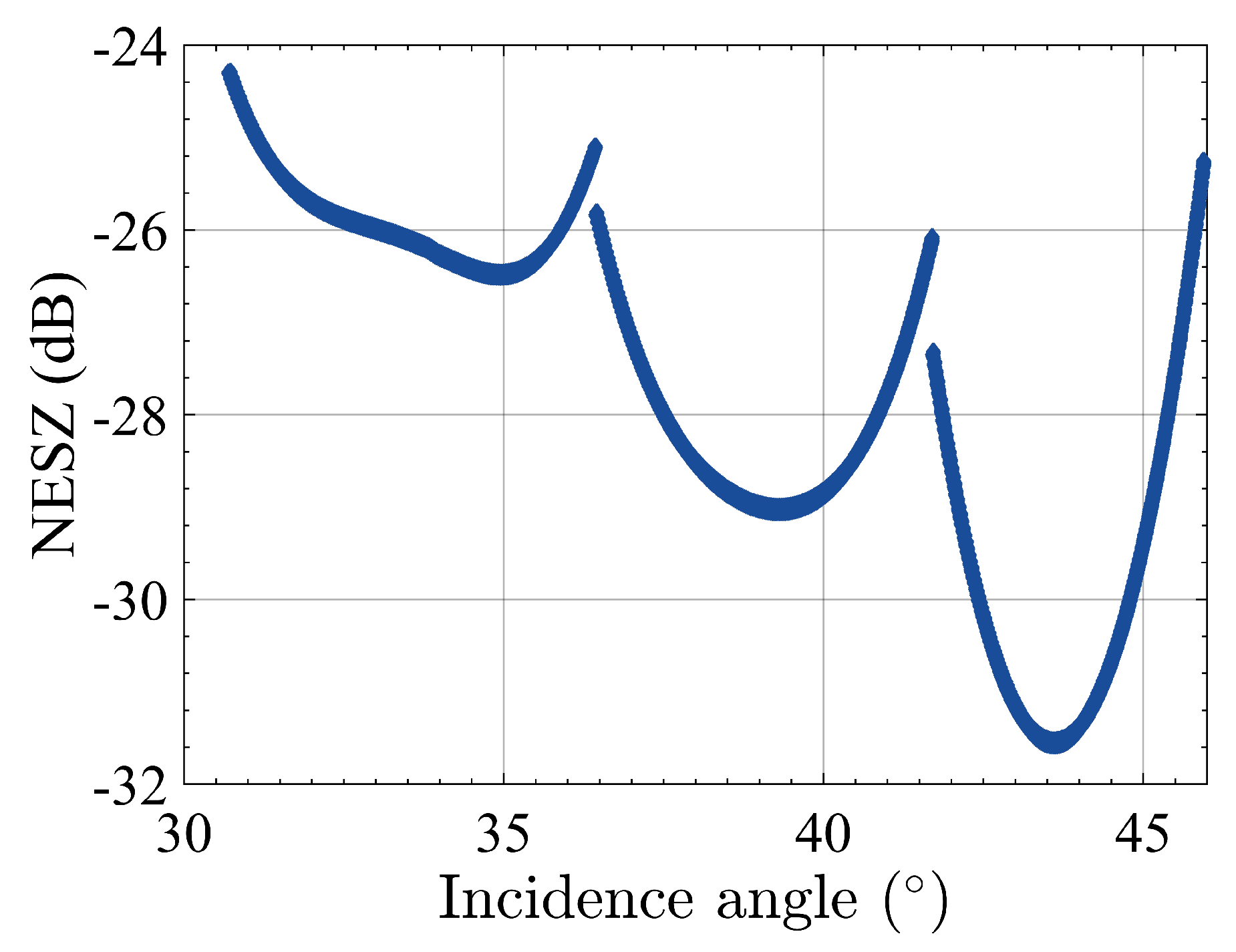
For the Sentinel-1 IW mode products, the nominal instrumental noise floors (i.e., the noise equivalent sigma naught (NESZ)) are calculated according to the formula provided in the Sentinel-1 product specification [31] and the metadata XML file contained in each product. The NESZ measures of IW mode VH polarization images with respect to incidence angles are plotted in Figure 1.
The noise removal is processed in two steps.
- Based on the calculated NESZ measures, data do not satisfy Equation (1) are removed.where denotes the NRCS in , and is the measured NESZ in . Empirical threshold is set to to guarantee the noise free signal is above , which is applicable for cross-pol wind analyses illustrated in [17]. Please note that, we do not apply higher cut-off level since we aimed at finding the minimum cross-pol NRCS for wind retrieval. Thus, some relatively low SNR data are reserved for further analyses.
- NRCS is composed of signal and noise which is particularly high for low SNR cross-pol observations. We attempt to subtract the noise component based on the calculated NESZ measures according to Equations (2)–(5) [15].where , , and denote the NRCS, the NESZ measures, and the noise free signal NRCS in linear scale. denotes the noise free signal NRCS in .
Based on the introduced steps of noise removal, an example of noise removal for Sentinel-IW GRD product is illustrated in Figure 2.
2.4. Experimental Data
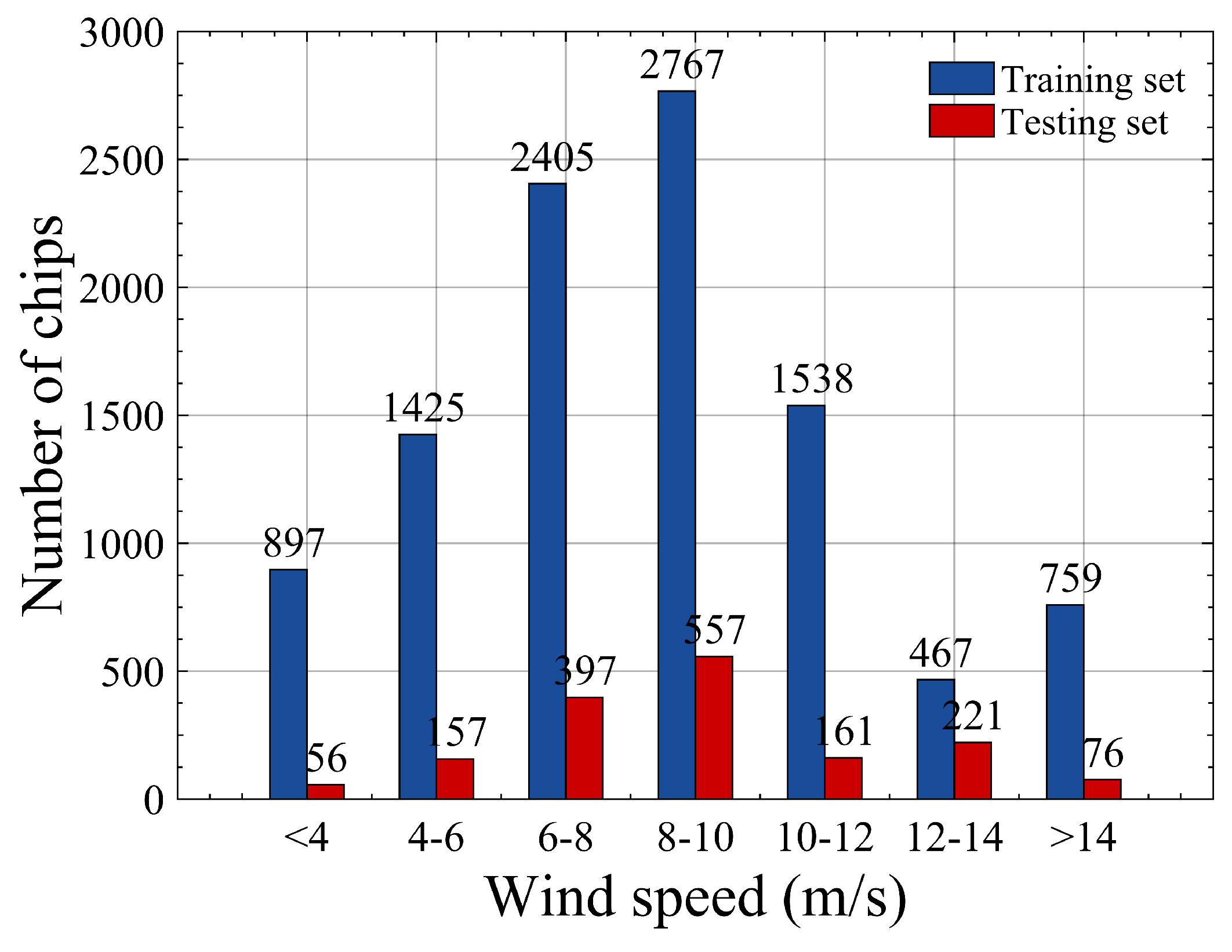
The 11,883 matchup data (noise removal) covering 90 Sentinel-1A and 1B VH dual-pol GRD images with precipitation. We divided the whole data into training and testing sets in two steps. First, the mathchup data are randomly divided into training set and testing set. Then in order to guarantee that both training and testing sets cover full ranges of incidence angles, wind directions and wind speeds, we manually adjust a small number of samples in the training and testing sets. After the two steps, the number of samples in training and testing sets are 10,258 and 1625, respectively. The distributions of wind speeds, wind directions, and incidence angles are shown in Figure 3, Figure 4 and Figure 5, respectively. The spatial distance error of the matchup data are shown in Figure 6. Here the spatial distance error is defined as the distance between the geographic position of the matchup ASCAT and the center of the corresponding SAR image.
3. Experiments and Analyses
3.1. Relationship between NRCS and Incidence Angles
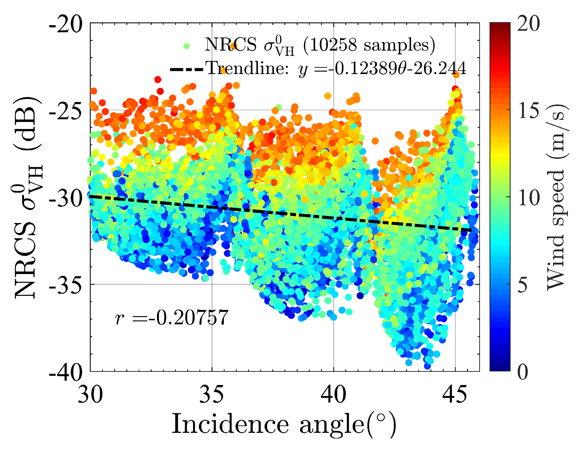
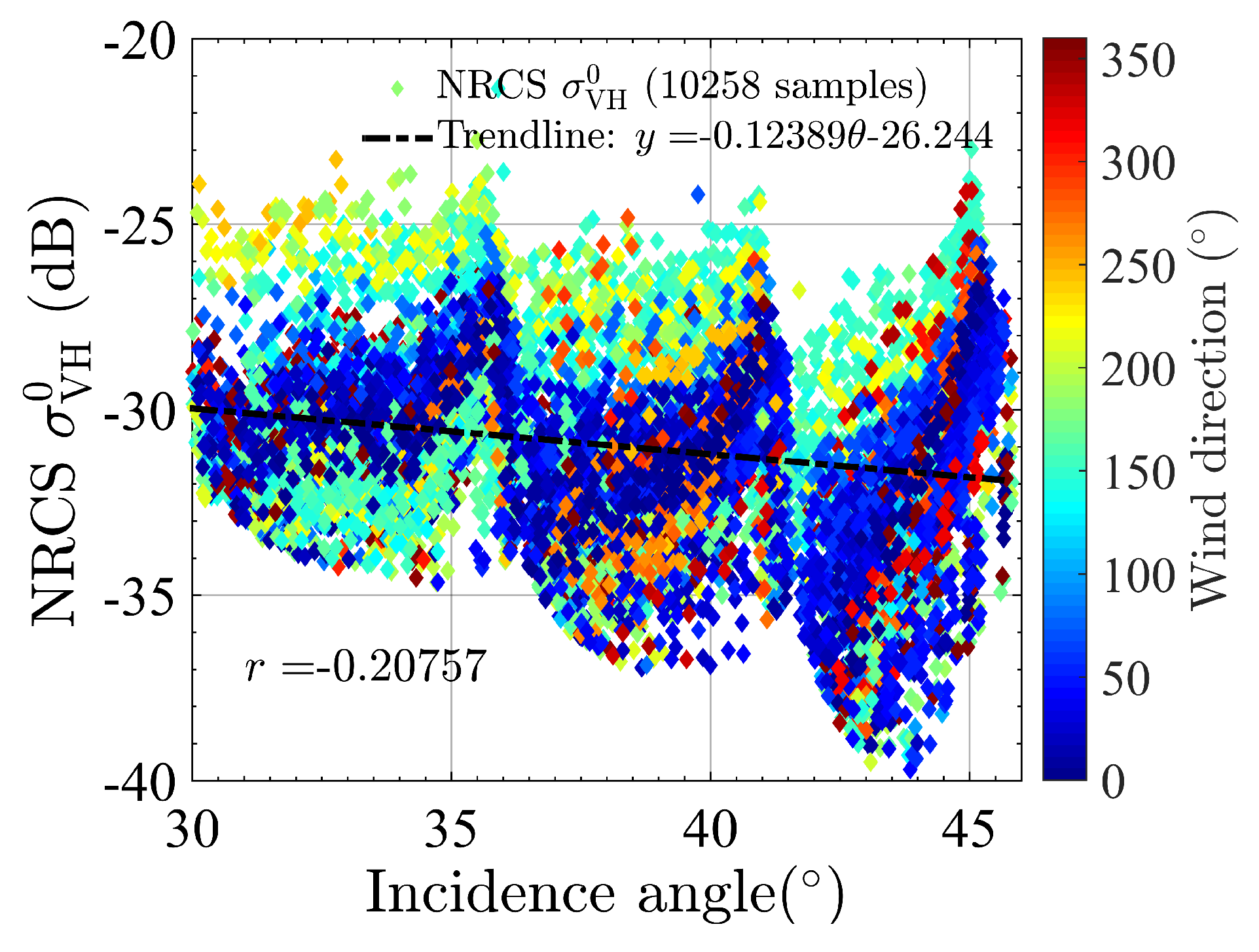
For the 12,058 training data and 1625 testing data, each SAR sub-image is integrated with environmental information, with the size of pixels ( resolution). The averaged value of the NRCS of SAR sub-image is calculated, denoted as . resolution is applicable and widely employed for SAR wind analyses [4,5,19]. Both Figure 7 and Figure 8 show the empirical relationship between the NRCS and incidence angle based on the 12,058 training data. In Figure 7, different colors represent the different values of wind speeds. Here, the wind direction is defined as the angle that lies between the true wind direction and the radar look direction. In addition, in Figure 8, different colors represent the different values of wind directions.
As illustrated in Figure 7 and Figure 8, because of the low SNR in cross-pol images, the radar backscattering is interfered with the instrumental noise. As such, the NRCS is fluctuated and negatively correlated to the incidence angles. The maximum wind speed in this dataset is .
From Figure 7, under every bin of incidence angles, the colors of data which represent different values of wind speeds are distinguishable. Known that the radar backscattering can reflect the ocean clutter more accurately when exceeding NESZ, from Figure 1 and Figure 7, it can be seen that the NRCS exceeds NESZ when the wind speed is roughly in the interval of about 8–10 . Moreover, under every bin of incidence angles, the colors of data are clearly distinguishable when wind speeds exceed the interval of 8–10 . While, the colors of the data are mixed-up when speed is below the interval of 8–10 , because in this condition, the radar backscattering of cross-pol are too low to reflect the ocean clutter. The accurate value of this wind speed threshold will be specified and discussed in Section 3.2.
From Figure 8, under every bin of incidence angles, the colors of data which represent different values of wind directions are scattered and mixed-up. However, we could not observe the wind direction dependence directly from this plot, since the wind direction dependence is relatively small for cross-pol [14,17]. The wind direction dependence will be quantitatively analyzed in Section 3.3.
3.2. Relationship between NRCS and Wind Speeds
In this section, we further analyzed the relationship between the NRCS and wind speeds. Due to the unique TOPSAR technique for the IW mode, three sub-swaths are captured, denoted as IW1-band (with incidence angles roughly ranging from to ), IW2-band (with incidence angles roughly ranging from to ), and IW3-band (with incidence angles roughly ranging from to ), respectively. Therefore, we categorized the 12,058 data according to their bands: IW1-band, IW2-band, and IW3-band.
3.2.1. IW1-Band
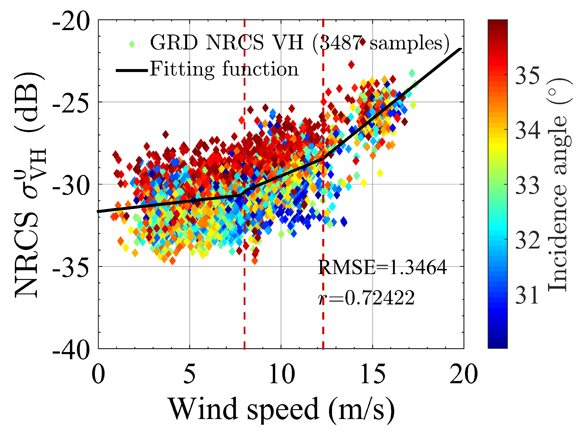
The relationship between the NRCS and wind speeds for IW1-band is illustrated in Figure 9. For the IW1-band, the range of incidence angles is 30–. Clearly, NRCS monotonically increase with wind speed. In the three regions (IW1-G1, IW1-G2 and IW1-G3) separated by dotted line representing 8 m/s and , the slope is constant and increases as wind speed increases. To quantify this relationship, a three piecewise-linear fitting is carried out, and the results of fitting are illustrated in Table 2.
For the IW1-G1 (wind speed is lower than ), the NRCS are scattered with large variation. This variation arises because the radar return signals are low, the NRCS can not reflect the backscattering of ocean clutter. In addition, from Table 2, the slope of fitting is .
For the IW1-G2 (wind speed is between and ), the variation of the decreases obviously. This indicates that when wind speed is higher than , for the Sentinel-1 cross-pol IW1 products, the radar backscattering is sensitive enough to reflect ocean clutter signatures when wind speed exceeds , and thus the wind speed retrieval from cross-pol observations is valid. This threshold is accordance with the analyses in the last paragraph of Section 3.1, in which we estimate the threshold to be 8–10 based on results Figure 1 and Figure 7. From Table 2, the slope of fitting is .
For IW1-G3 (wind speed is above ), the slope of the fitting function obviously increases. From Table 2, the slope of fitting is , indicating the higher rate of increase of the NRCS with wind speeds. In the research of RADARSAT-2 VH dual-polarization images [15], Shen et al. also referred to this turning point estimated at about . This phenomena is theoretically explained as the wave-breaking contributions by non-bragg surface scattering mechanisms or volume scattering from breaking generated foamy layers, by Hwang et al. in [7,14]. Therefore, the wind speed sensitivity, as reflected in slope, increases with higher wind speeds, which suggests the potential of Sentinel-1 cross-pol for higher wind retrievals. Here, noted that due to the limitation of maximum wind speed of ASCAT products, the signal saturation of Sentinel-1 cross-pol will be further investigated in the future.
3.2.2. IW2-Band
The relationship between the NRCS and wind speeds for IW2-band is illustrated in Figure 10. For the IW2-band, the range of incidence angles is 36–. Similarly, the relationship between the NRCS and wind speeds has the same trends as these in IW-1 band. Therefore, according to the slopes, the data can be divided into two groups, denoted as IW2-G1, IW2-G2, which are separated by wind speed at , marked in the dotted line. To quantify this relationship, a two piecewise-linear fitting is carried out, and the results of fitting are illustrated in Table 2.
For IW2-G1, when the wind speed is lower than , the are scattered with large variation, and from Table 2, the slope of fitting is . As discussed in Section 3.2.1, this variation arises because the radar return signals are too low to reflect the backscattering of ocean clutter signatures accurately. For IW2-G2, when the wind speed is higher than , the variation of the decreases obviously. This indicates that when wind speed is higher than , the radar return signals are sensitive enough to reflect ocean clutter signatures, and thus the wind speed retrieval from cross-pol observations is valid. Due to the limitation of the maximum wind speed is under , there suggests no turning point of significant change of slope. Because of the higher incidence angle of IW2-band, this point may occur at larger wind speed than that of IW1-band ().
3.2.3. IW3-Band
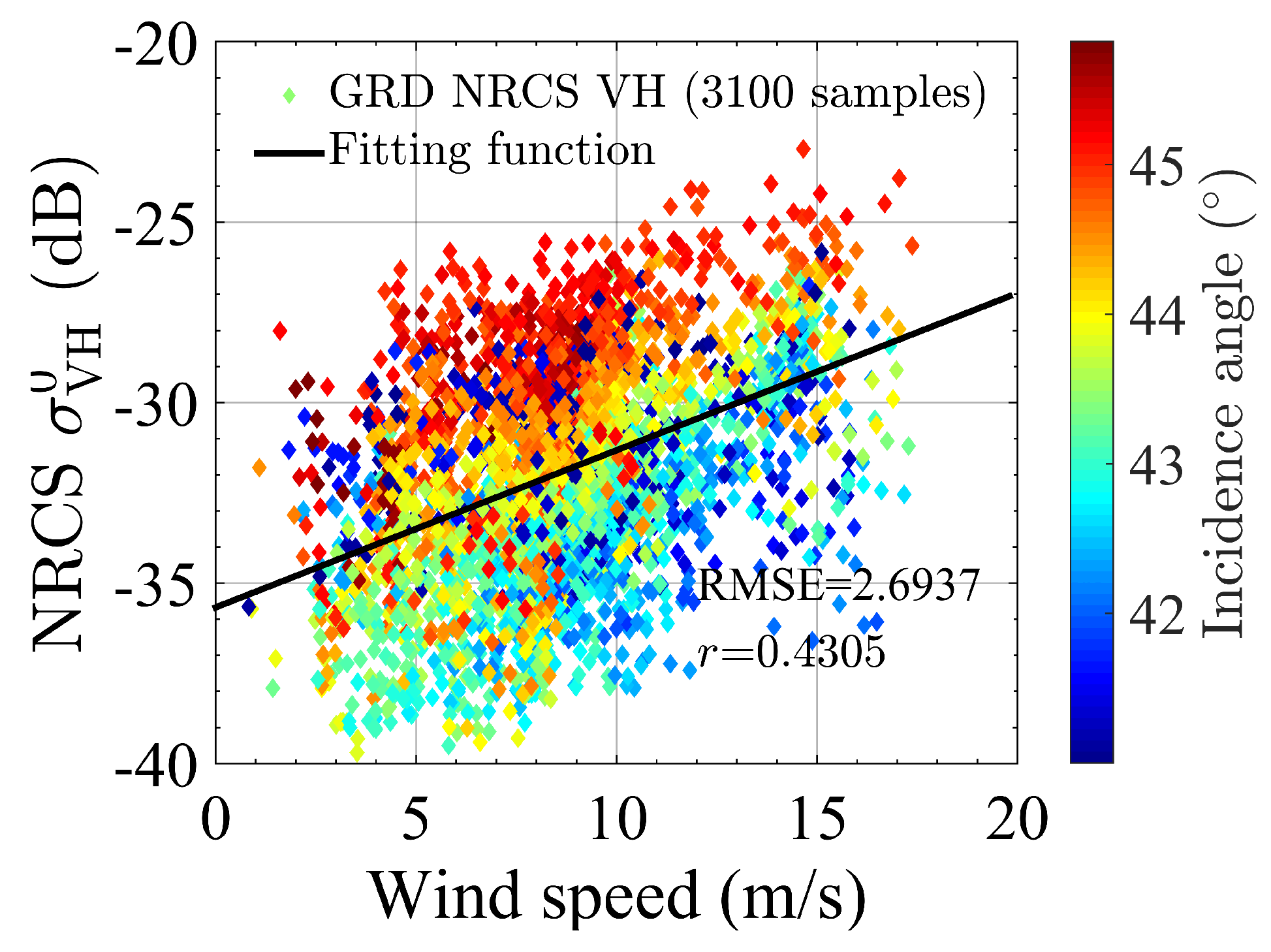
The relationship between the NRCS and wind speeds for IW3-band is illustrated in Figure 11. For the IW3-band, the range of incidence angles is 41–. To quantify the relationship, a linear fitting is carried out, and the results of fitting are illustrated in Table 2. For IW3-band, due to the higher incidence angles, the NRCS are relatively lower. The data are scattered, and the correlation coefficient r is very low. This observation of Sentinel-1 is consistent with [32]. Based on the data of ASAR AP mode, compared with higher incidence angles, Vachon et al. conclude that the cross-pol radar returns can better reflect the signatures of clutter in lower incidence angles [32]. Therefore, we infer that for the IW3-band, the NRCS can not reflect the radar backscattering of ocean clutter signatures, and the accuracy of wind retrieval can not be guaranteed in moderate wind conditions (<20 ).
3.3. Relationship between NRCS and Wind Directions
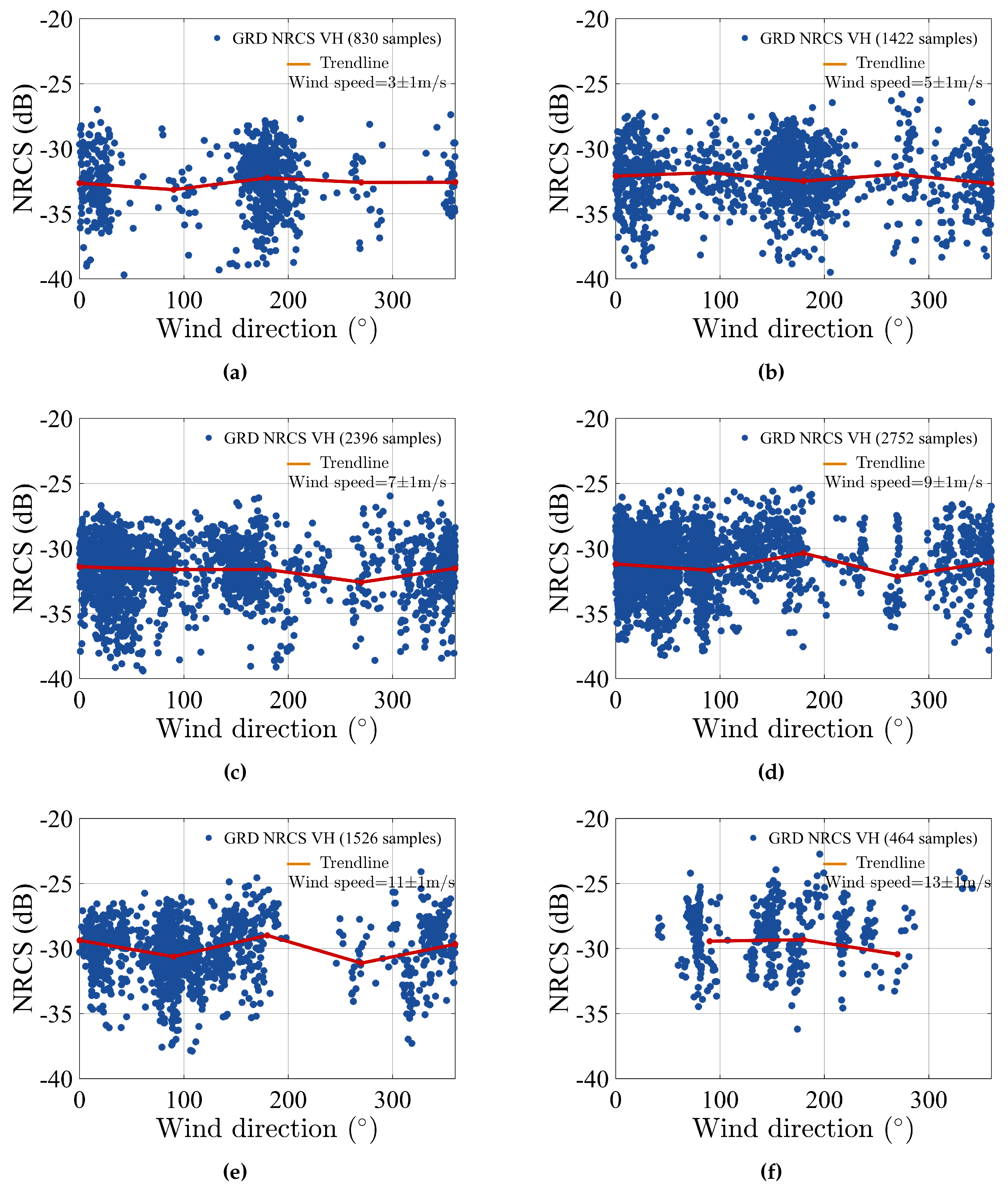
As illustrated in Section 3.1, wind speed performs more significant effects on NRCS than wind direction. Therefore, to determine the dependence of NRCS with respect to wind direction, the effects of wind speed should be isolated [17]. In this section, the NRCS are investigated for wind speeds at 3, 5, 7, 9, 11 and bounded by interval. The relationships between NRCS and wind direction for different wind speed intervals are illustrated in Figure 12. For each subfigure, the mean values of NRCS are calculated for wind directions at , , , and bounded by interval. The mean values are illustrated in Table 3. In addition, in Figure 12, the mean values are presented in red points and connected into the red lines to show the trend of NRCS variation with respect to different wind directions. Note that the range of wind direction is , thus the mean values of NRCS at and are calculated in and intervals, respectively. Besides, because of the deficiency of data at for and intervals, their mean values of NRCS are not calculated.
From Figure 12, the dependence on wind directions is visible. The values of NRCS reach local maxima at the up- and downwind directions (, and ) and local minima at the crosswind directions ( and ). This observation is consistent with the recent studies [14,17], which indicated wind direction dependence for cross-pol NRCS. It should be noted that for the interval of wind speed at and , the wind dependences of NRCS are not obvious. This can be explained as the relatively low SNR of radar signal returns in low wind conditions, which has been detailed in Section 3.1 and Section 3.2. Based on Table 3, the average variation between the NRCS at the up-/downwind directions and the crosswind is about for wind speed exceeds . Horstmann et al. [17] indicate that the wind direction dependence decreases with the increasing wind, and the direction dependence loses when speed exceeds . In this section, because of the limited data in high wind condition, this observation is not presented. We will handle with this problem in the future work.
3.4. Summary
Based on the theoretical and empirical researches developed on RADARSAT-2, and considering the unique characteristics of Sentinel-1 IW mode, the relationship between the NRCS and wind speeds with attention to evaluate contribution from incidence angle and wind direction terms are analyzed in Section 3.1, Section 3.2 and Section 3.3. After analyses, six observations are made.
- For Sentinel-1 cross-pol images, the radar backscattering NRCS are fluctuated and negatively correlated with the incidence angles.
- For Sentinel-1 cross-pol images, the values of NRCS reach local maxima at the up- and downwind directions (, and ) and local minima at the crosswind directions ( and ). In addition, the average variation between the NRCS at the up-/downwind directions and the crosswind is about in our experiment.
- Due to the unique TOPSAR technique for the IW mode (three sub-swaths IW1, IW2, IW3), the relationship between the NRCS and wind speeds for three sub-swaths are different and should be analyzed respectively.
- For IW1-band, the relationship between the NRCS and wind speeds is monotonically linear increase, and the slope increases with higher wind speeds. The data can be divided into three groups. When the wind speed is lower than , the NRCS are scattered with large variation because the radar returns are low. When the wind speed is between and , the variation of the NRCS decreases obviously. This indicates the radar backscattering is sensitive enough to reflect ocean clutter signatures, and thus the wind speed retrieval from cross-pol observations is valid. When the wind speed is above , the wind speed sensitivity, as reflected in slope, increases with higher wind speeds, suggesting the potential of Sentinel-1 cross-pol to high wind retrievals.
- For the IW2-band, the relationship between the NRCS and wind speeds is monotonically linear increase. When the wind speed is lower than , the NRCS are scattered with large variation because the radar return signals are low. When the wind speed is higher than , the variation of the NRCS decreases obviously. The radar backscattering is sensitive enough to reflect ocean clutter signatures, and thus the wind speed retrieval from cross-pol observations is valid.
- For the IW3-band, due to the higher incidence angles, we infer that for IW3-band, the NRCS can not reflect the radar backscattering of ocean clutter signatures, and the accuracy of wind retrieval can not be guaranteed in moderate wind condition (<20).
The meaning of these analyses is that by revisiting the theoretical and empirical relationship derived from RADARSAT-2 data, we assess the Sentinel-1 IW cross-pol images, and provide a technical evaluation on ocean wind retrieval from Sentinel-1 cross-pol images. In summary, for Sentinel-1 IW products, the NRCS can better reflect the ocean clutter signatures in relatively lower incidence angles, which is IW1-band and IW2-band, therefore are suitable for wind field retrieval when wind speed exceeds the low boundary ( and for IW1 and IW2 band, respectively). An empirical model based on this is proposed in the next section.
4. Proposed Model for Sentinel-1 Cross-Pol Wind Retrieval
Based on the analyses in Section 3, we infer the NRCS is dependent on incidence angle, wind speed and wind direction. Therefore, we propose a model to describe this relationship for Sentinel-1 cross-pol IW images.
where denotes the NRCS values of radar return signals in , is defined as weight parameter, C is the constant, is the wind speed function which describes the relationship between the NRCS and wind speed, is the incidence angle function normalized into , A is to compensate the effects of wind direction. Both and are obtained from the observational data by fitting functions. The applicable condition of the proposed model will be given in Equations (7) and (9) in next sections.
4.1. Wind Speed Function
Based on the analyses in Section 3.2, under specific condition of incidence angles and wind speeds, the radar return signals can be utilized to retrieve wind filed. Specifically, for IW1-band (incidence angle between and ) and for IW2-band (incidence angle between and ), wind speed retrievals can be performed when wind speeds exceed and , respectively. Base on Table 2, the wind speed function is proposed as
4.2. Wind Direction Compensation
For Sentinel-1 cross-pol images, the values of NRCS reach local maxima at the up- and downwind directions (, and ) and local minima at the crosswind directions ( and ). In addition, the average variation between the NRCS at the up-/downwind directions and the crosswind is about in our experiment. Therefore, for simplicity, A is empirically set according to Equation (8) to compensate the effects of wind direction.
4.3. Incidence Angle Function
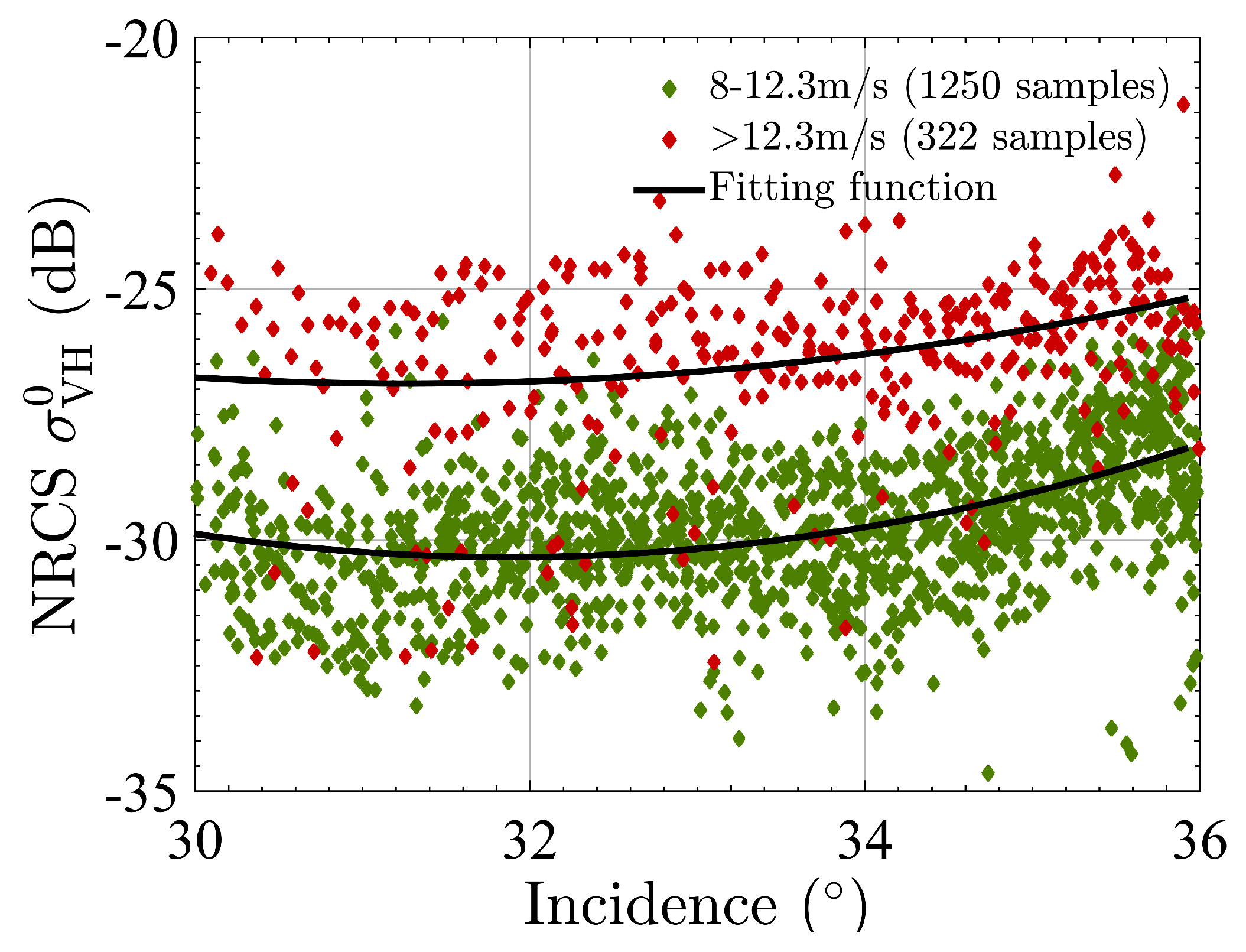
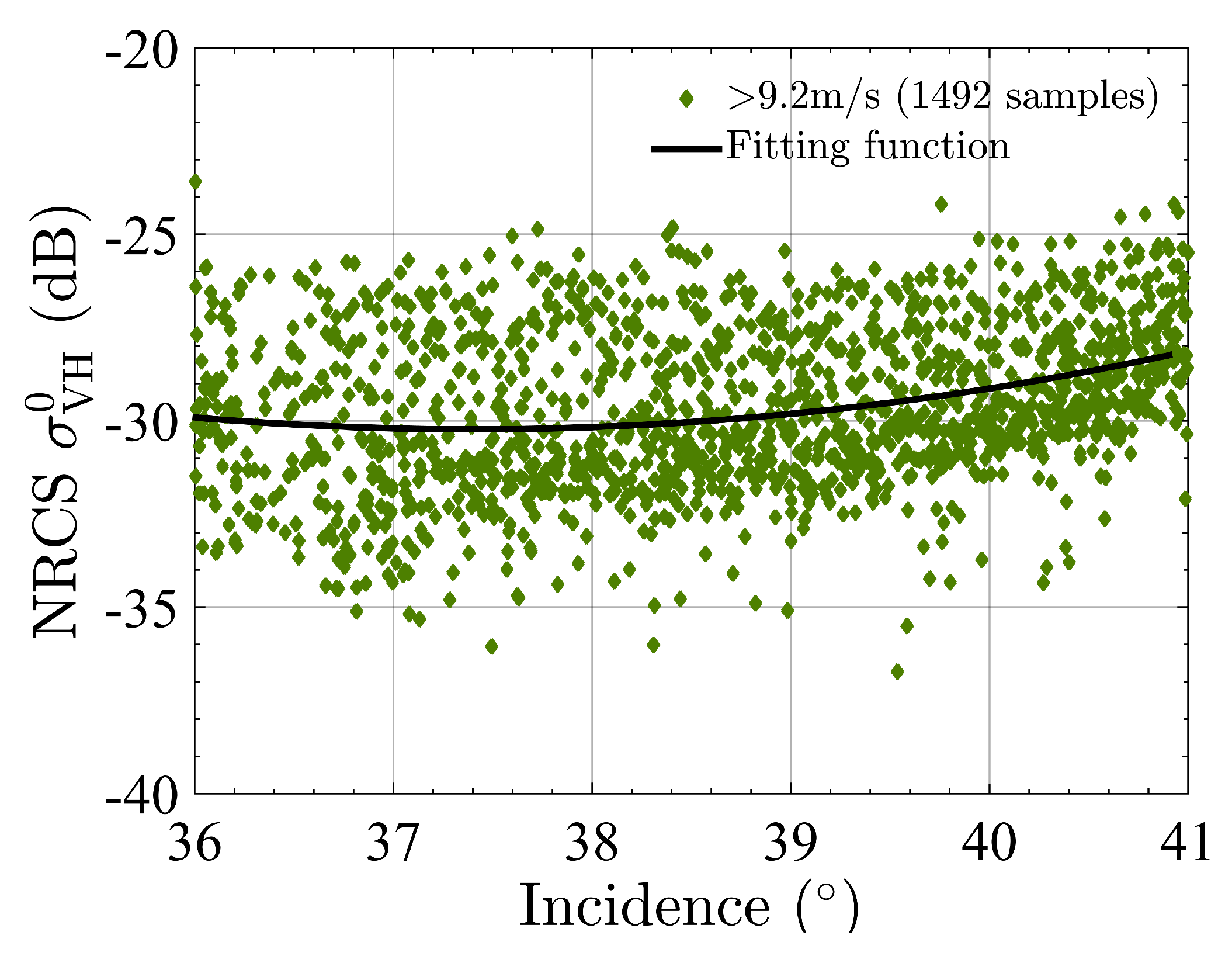
Based on the analyses of Section 3.1, for IW1-band (incidence angle between and ) wind speed retrieval can be performed when wind speed exceeds , and the slope increase obviously when wind speed exceed . For the IW2-band (incidence angle between and ), wind speed retrieval can be performed when wind speed exceeds . Therefore, for the three subgroups of data, 2 degree polynomial functions are employed to fitting the data, illustrated in Figure 13 and Figure 14.
The incidence angle function is proposed as
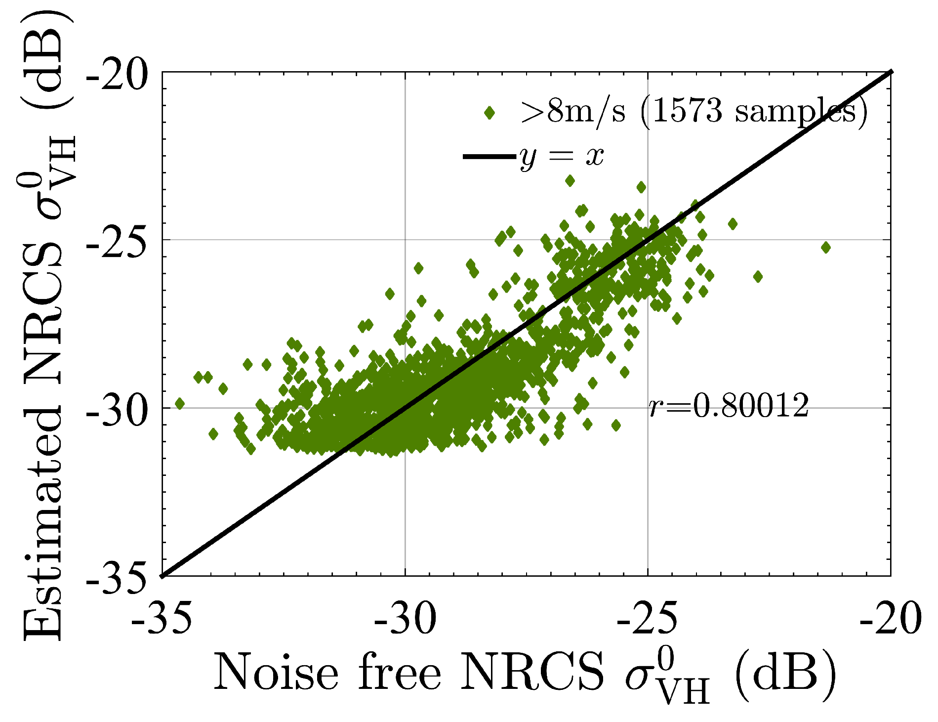
By substituting Equations (7) and (9) into Equation (6), we get the model to describe this relationship for Sentinel-1 IW cross-pol images. The parameters of the proposed model corresponding to different situations are listed in Table 4. Figure 15 and Figure 16 illustrate the performance of the proposed model. The correlation coefficient and are and for IW1 and IW2 band, respectively, which are improved by taking the dependence on incidence angle, wind speed and wind direction into consideration.
4.4. Model Validation
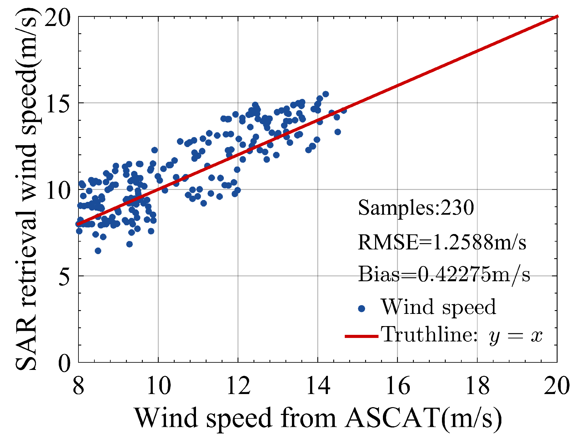
As introduced in Section 2.4, the testing dataset which were not used to derive Equation (6) contains 1625 data covering full ranges of incidence angles, wind speeds and wind directions. Since the applicable condition of the proposed model are given in Equations (7) and (9), 230 data which satisfy this condition are selected from the testing dataset. Based on Equation (6), the retrieved wind speeds from Sentinel-1 IW cross-pol images compared with the ASCAT measurements are illustrated in Figure 17. The bias of the retrieved wind speed is , and the root mean square error (RMSE) is . Besides, from Figure 17, the accuracy of retrievals increases in high speed condition. For wind speed higher than , the bias and RMSE are and , respectively. This may be due to less accurate radar return signals in low-to-moderate wind condition. As Vachon and Wolf suggested in [12], the higher noise floor is, the larger wind speed is required to guarantee the useful radar backscattering which accurately reflect ocean clutter signatures.
In order to further demonstrate the suitability of the proposed model, a model proposed by Shen et al. based on RADARSAT-2 ScanSAR cross-pol data is carried out for comparison [15]. Shen’s model is a two piecewise-linear function proposed as
where v is the wind speed. and the two line segments meet when the wind speed is . Similarly, we first estimate NRCS by Shen’s model and calculate the correlation coefficient and for IW1 and IW2 band, respectively. Then, the wind filed retrieval is carried out on same testing dataset and the bias and RMSE are calculated. The detailed performances comparison are shown in Table 5.
As we can see from Table 5, the proposed model shows better performance, for larger values of and and smaller values of Bias and RMSE. In [15], Shen et al. indicate that show no evident dependence on incidence angles or wind direction, therefore the model only took wind speed into consideration, and performed very good wind retrieval ability for hurricane. In this experiment, for moderate wind condition, the show dependences on incidence angles and wind directions. Therefore, the proposed model which considers the dependences on incidence angle, wind speed and wind direction performs better.
5. Discussion
5.1. Influence of Different Samples of Training and Testing Sets
Based on the 10,258 matchup data as training dataset, we analyzed the dependences of with respect to incidence angles, wind speeds, and wind directions, and proposed a model for wind retrieval. However, different sets of samples for training and testing might cause undesirable effects on fitting results, thus the stability and performance of the model might be affected. In this section, in order to evaluate this effect, we carried out all the experiments in Section 3 and Section 4 with different samples in training dataset and testing dataset. The results are summarized in Table 6 and Table 7.
As shown in Table 6, dataset 1 is composed of 12,058 for training and 1625 for testing, which is employed in the former sections of this paper. Both the training and testing data cover full ranges of incidence angles, wind speeds and wind directions. Dataset 2 is composed of 9285 for training and 2598 for testing, which is employed for comparison. Both the training and testing data cover full ranges of incidence angles, wind speeds and wind directions. Dataset 3 is composed of 8134 for training and 3797 for testing, which is employed for comparison. Both the training and testing data cover full ranges of incidence angles, wind speeds and wind directions. Table 6 summarized the parameters of the proposed model for different sets of samples. As we can observe, most of the coefficients in the model maintain relatively stable for three different datasets. Thus, we infer that the effects of training samples on model deriving are not significant.
Based on Equation (6), the performances of the proposed model for the three different datasets are summarized in Table 7. For dataset 1–3, 230, 335, 917 data which satisfy the applicable condition (given in Equations (7) and (9)) are selected from the testing dataset and performed wind field retrievals, respectively. Table 7 summarized the performances of the proposed model for three different datasets. As we can observe, most of the measurements maintain relative stability. Thus, we infer that the effects of testing samples on wind retrieval are not significant.
5.2. Influence of Different Number of Pixels for SAR Chip
The experiments in Section 3 and Section 4 are carried out on SAR chips with the size of pixels ( resolution). Therefore, for each matchup data, is calculated as the averaged value of the NRCS of pixels. However, the different number of samples for average might cause undesirable effects on fitting results, thus the stability and performance of the model might be affected. In this section, in order to evaluate this effect, we carried out all the experiments in Section 3 and Section 4 with different number of samples for average. The results are summarized in Table 8 and Table 9.
Table 8 summarized the parameters of the proposed model for different number of averaged pixels: , and pixels. As we can observe, most of the coefficients in the model maintain relatively stable with different pixel numbers. Thus, we infer that the effects of pixel numbers on model deriving are not significant. Based on Equation (6), the performances of the proposed model for different number of averaged pixels are summarized in Table 9. As we can observe, most of the measurements maintain relatively stable. Thus, we infer that the effects of pixel numbers on wind retrieval are not significant.
6. Conclusions
In this paper, we revisit the empirical relationships between cross-pol radar backscattering and wind speeds with attention to evaluate contribution from incidence angle and wind direction terms. The scopes of this paper are to give a technical evaluation of Sentinel-1 cross-pol images based on the theoretical and empirical analyses derived from RADARSAT-2 data, and provide a wind retrieval model based on Sentinel-1 cross-pol images.
In order to better understand the Sentinel-1 cross-pol NRCS values under various environmental conditions, we construct a dataset by matching SAR winds with near coincide wind vectors from ASCAT scatterometer. 11,883 data with precipitation are utilized as training and testing data in the following analyses.
Next, we calculate the NESZ of Sentinel-1 IW mode, and perform noise removal for all the matchup data. Empirical relationships among the noise free NRCS , wind speed, wind direction, and radar incidence angle are analyzed. The lowest boundary wind speed for retrievals is specified.
A piecewise model particularly fitting the Sentinel-1 IW mode is proposed to describe the relationships between the NRCS and factors. The model is composed of the incidence angle function, wind speed function and wind direction compensation, derived from data fitting. Compared with the analyses of incidence angle and wind speed separately in Section 3, the larger r suggests the necessity of taking incidence angle, wind speed and wind direction into consideration for describing this relationship. In addition, the model is validated using 230 data. The low bias and RMSE show the suitability of the proposed model for Sentinel-1 IW cross-pol images. Furthermore, the retrieval accuracy of the model increases in high speed condition; for smaller bias and RMSE with higher wind speeds. This indicates the potential of apply Sentinel-1 cross-pol images to wind retrievals in extreme weather.
Future work involves further analyzing the Sentinel-1 cross-pol radar backscattering with incidence angles and wind speeds in very high wind conditions. The signal saturation of Sentinel-1 cross-pol images will be further investigated, because there are not enough high-wind matchup data available as of now. However, we expect that there will be more Sentinel-1 images covering hurricanes/typhoons as shown in [33] in the coming years, and we will be able to validate the model against airborne and spaceborne sensors special designed for high-wind measurements. Moreover, we will match Sentinel data with buoys and do more validation and modification of the model against multiple wind products.
Acknowledgments
This work was supported by the State Key Program of the National Natural Science Foundation of China under Grant 61331015. The authors would also like to thank the European Space Agency for providing the Sentinel-1 data and the SNAP 4.0, JPL for the ASCAT data, and Precipitation Measurement Missions, NASA for the TRMM data. The views, opinions, and findings contained in this paper are those of the authors and should not be construed as an official NOAA or U.S. government position, policy, or decision.
Author Contributions
Lanqing Huang and Bin Liu conceived and performed the experiments. Bin Liu and Xiaofeng Li supervised and designed the research and contributed to the organization of article. Lanqing Huang drafted the manuscript, and all authors revised and approved the final version of the manuscript.
Conflicts of Interest
The authors declare no conflict of interest.
References
- Hersbach, H. CMOD5: An Improved Geophysical Model Function for ERS C-Band Scatterometry; European Centre for Medium-Range Weather Forecasts: Reading, UK, 2003. [Google Scholar]
- Xu, Q.; Lin, H.; Li, X.; Zuo, J.; Zheng, Q.; Pichel, W.G.; Liu, Y. Assessment of an analytical model for sea surface wind speed retrieval from spaceborne SAR. Int. J. Remote Sens. 2010, 31, 993–1008. [Google Scholar] [CrossRef]
- Wackerman, C.C.; Clemente-Colón, P.; Pichel, W.G.; Li, X. A two-scale model to predict C-band VV and HH normalized radar cross section values over the ocean. Can. J. Remote Sens. 2002, 28, 367–384. [Google Scholar] [CrossRef]
- Yang, X.; Li, X.; Pichel, W.G.; Li, Z. Comparison of ocean surface winds from ENVISAT ASAR, MetOp ASCAT scatterometer, buoy measurements, and NOGAPS model. IEEE Trans. Geosci. Remote Sens. 2011, 49, 4743–4750. [Google Scholar] [CrossRef]
- Yang, X.; Li, X.; Zheng, Q.; Gu, X.; Pichel, W.G.; Li, Z. Comparison of ocean-surface winds retrieved from QuikSCAT scatterometer and Radarsat-1 SAR in offshore waters of the US west coast. IEEE Geosci. Remote Sens. Lett. 2011, 8, 163–167. [Google Scholar] [CrossRef]
- Liu, G.; Yang, X.; Li, X.; Zhang, B.; Pichel, W.; Li, Z.; Zhou, X. A systematic comparison of the effect of polarization ratio models on sea surface wind retrieval from C-band synthetic aperture radar. IEEE J. Sel. Top. Appl. Earth Obs. Remote Sens. 2013, 6, 1100–1108. [Google Scholar] [CrossRef]
- Hwang, P.A.; Zhang, B.; Toporkov, J.V.; Perrie, W. Comparison of composite Bragg theory and quad-polarization radar backscatter from RADARSAT-2: With applications to wave breaking and high wind retrieval. J. Geophys. Res. Oceans 2010, 115. [Google Scholar] [CrossRef]
- Zhang, B.; Perrie, W.; Vachon, P.W.; Li, X.; Pichel, W.G.; Guo, J.; He, Y. Ocean vector winds retrieval from C-band fully polarimetric SAR measurements. IEEE Trans. Geosci. Remote Sens. 2012, 50, 4252–4261. [Google Scholar] [CrossRef]
- Zhang, B.; Li, X.; Perrie, W.; He, Y. Synergistic measurements of ocean winds and waves from SAR. J. Geophys. Res. Oceans 2015, 120, 6164–6184. [Google Scholar] [CrossRef]
- Kim, T.S.; Park, K.A.; Li, X.; Mouche, A.A.; Chapron, B.; Lee, M. Observation of Wind Direction Change on the Sea Surface Temperature Front Using High-Resolution Full Polarimetric SAR Data. IEEE J. Sel. Top. Appl. Earth Obs. Remote Sens. 2017, 10, 2599–2607. [Google Scholar] [CrossRef]
- Zhang, G.; Li, X.; Perrie, W.; Hwang, P.A.; Zhang, B.; Yang, X. A Hurricane Wind Speed Retrieval Model for C-Band RADARSAT-2 Cross-Polarization ScanSAR Images. IEEE Trans. Geosci. Remote Sens. 2017, 55, 4766–4774. [Google Scholar] [CrossRef]
- Vachon, P.W.; Wolfe, J. C-band cross-polarization wind speed retrieval. IEEE Geosci. Remote Sens. Lett. 2011, 8, 456–459. [Google Scholar] [CrossRef]
- Bergeron, T.; Bernier, M.; Chokmani, K.; Lessard-Fontaine, A.; Lafrance, G.; Beaucage, P. Wind speed estimation using polarimetric RADARSAT-2 images: Finding the best polarization and polarization ratio. IEEE J. Sel. Top. Appl. Earth Obs. Remote Sens. 2011, 4, 896–904. [Google Scholar] [CrossRef]
- Hwang, P.A.; Perrie, W.; Zhang, B. Cross-polarization radar backscattering from the ocean surface and its dependence on wind velocity. IEEE Geosci. Remote Sens. Lett. 2014, 11, 2188–2192. [Google Scholar] [CrossRef]
- Shen, H.; Perrie, W.; He, Y.; Liu, G. Wind speed retrieval from VH dual-polarization RADARSAT-2 SAR images. IEEE Trans. Geosci. Remote Sens. 2014, 52, 5820–5826. [Google Scholar] [CrossRef]
- Zhang, B.; Perrie, W.; Zhang, J.A.; Uhlhorn, E.W.; He, Y. High-resolution hurricane vector winds from C-band dual-polarization SAR observations. J. Atmos. Ocean. Technol. 2014, 31, 272–286. [Google Scholar] [CrossRef]
- Horstmann, J.; Falchetti, S.; Wackerman, C.; Maresca, S.; Caruso, M.J.; Graber, H.C. Tropical cyclone winds retrieved from C-band cross-polarized synthetic aperture radar. IEEE Trans. Geosci. Remote Sens. 2015, 53, 2887–2898. [Google Scholar] [CrossRef]
- Zecchetto, S.; De Biasio, F.; della Valle, A.; Quattrocchi, G.; Cadau, E.; Cucco, A. Wind Fields From C-and X-Band SAR Images at VV Polarization in Coastal Area (Gulf of Oristano, Italy). IEEE J. Sel. Top. Appl. Earth Obs. Remote Sens. 2016, 9, 2643–2650. [Google Scholar] [CrossRef]
- Monaldo, F.; Jackson, C.; Li, X.; Pichel, W.G. Preliminary evaluation of Sentinel-1A wind speed retrievals. IEEE J. Sel. Top. Appl. Earth Obs. Remote Sens. 2016, 9, 2638–2642. [Google Scholar] [CrossRef]
- Agency, C.S. RADARSAT Constellation. Available online: http://www.asc-csa.gc.ca/eng/satellites/radarsat/default.asp (accessed on 1 September 2015).
- Flett, D.; Crevier, Y.; Girard, R. The RADARSAT Constellation Mission: Meeting the government of Canada’S needs and requirements. In Proceedings of the 2009 IEEE International Geoscience and Remote Sensing Symposium, Cape Town, South Africa, 12–17 July 2009; Volume 2, pp. 907–910. [Google Scholar]
- Thompson, A.A. Innovative capabilities of the RADARSAT constellation mission. In Proceedings of the 8th European Conference on Synthetic Aperture Radar, Aachen, Germany, 7–10 June 2010; pp. 1–3. [Google Scholar]
- Global, OSI. ASCAT Wind Product User Manual. Available online: http://projects.knmi.nl/scatterometer/publications/pdf/ASCAT_Product_Manual.pdf (accessed on 1 September 2013).
- Torres, R.; Snoeij, P.; Geudtner, D.; Bibby, D.; Davidson, M.; Attema, E.; Potin, P.; Rommen, B.; Floury, N.; Brown, M.; et al. GMES Sentinel-1 mission. Remote Sens. Environ. 2012, 120, 9–24. [Google Scholar] [CrossRef]
- European Space Agency, Sentinel-1 Team. Sentinel-1 User Handbook. Available online: http://sentinel.esa.int/ (accessed on 1 September 2013).
- ESA. Copernicus Open Access Hub. Available online: https://scihub.copernicus.eu/ (accessed on 1 September 2014).
- NASA EOSDIS PO.DAAC. Physical Oceanography Distributed Active Archive Center (PO.DAAC). Available online: https://podaac.jpl.nasa.gov/ (accessed on 1 September 2015).
- ESA. Step Science Toolbox Explotiation Platform. Available online: http://step.esa.int/main/toolboxes/snap/ (accessed on 1 September 2014).
- Missions, P.M. TRMM Data Download. Available online: https://pmm.nasa.gov/index.php?q=data-access/downloads/trmm (accessed on 1 September 2015).
- Huffman, G.J.; Bolvin, D.T. TRMM and Other Data Precipitation Data Set Documentation. Available online: https://pmm.nasa.gov/sites/default/files/document_files/3B42_3B43_doc_V7_4_19_17.pdf (accessed on 1 September 2017).
- European Space Agency, Sentinel-1 Team. Sentinel-1 Product Specification. Available online: https://sentinels.copernicus.eu/web/sentinel/user-guides/sentinel-1-sar/document-library/-/asset_publisher/1dO7RF5fJMbd/content/sentinel-1-product-specification (accessed on 1 November 2016).
- Vachon, P.W.; Wolfe, J. GMES Sentinel-1 Analysis of Marine Applications Potential (AMAP); DRDC Ottawa ECR: Ottawa, ON, Canada, 2008; Volume 218. [Google Scholar]
- Li, X. The first Sentinel-1 SAR image of a typhoon. Acta Oceanol. Sin. 2015, 34, 1–2. [Google Scholar] [CrossRef]
Figure 1.
NESZ measures for IW mode VH images.

Figure 2.
NRCS in radar range direction (blue) with and (green) without noise removal.
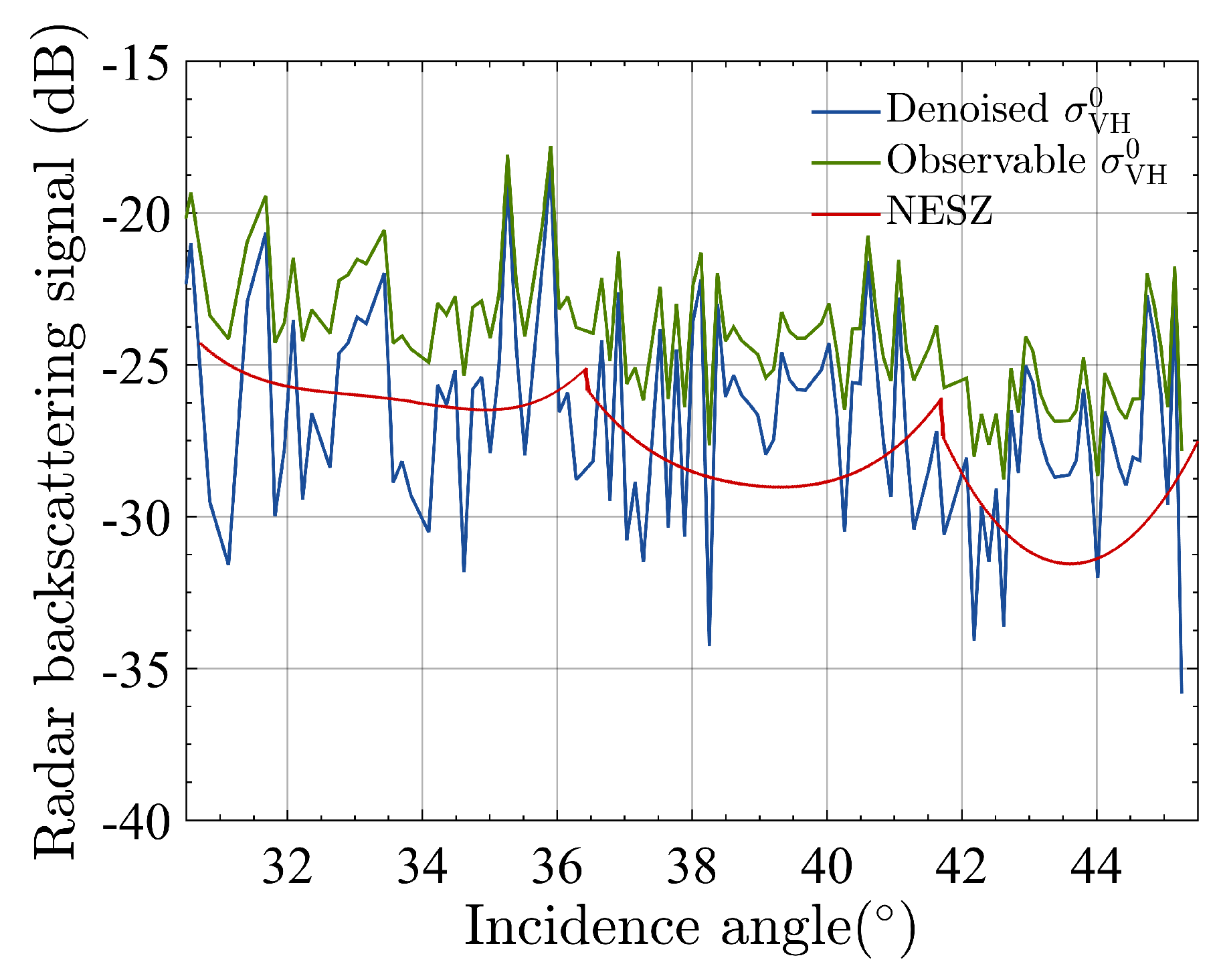
Figure 3.
Wind speed histogram of the matchup dataset.

Figure 4.
Wind direction histogram of the matchup dataset.
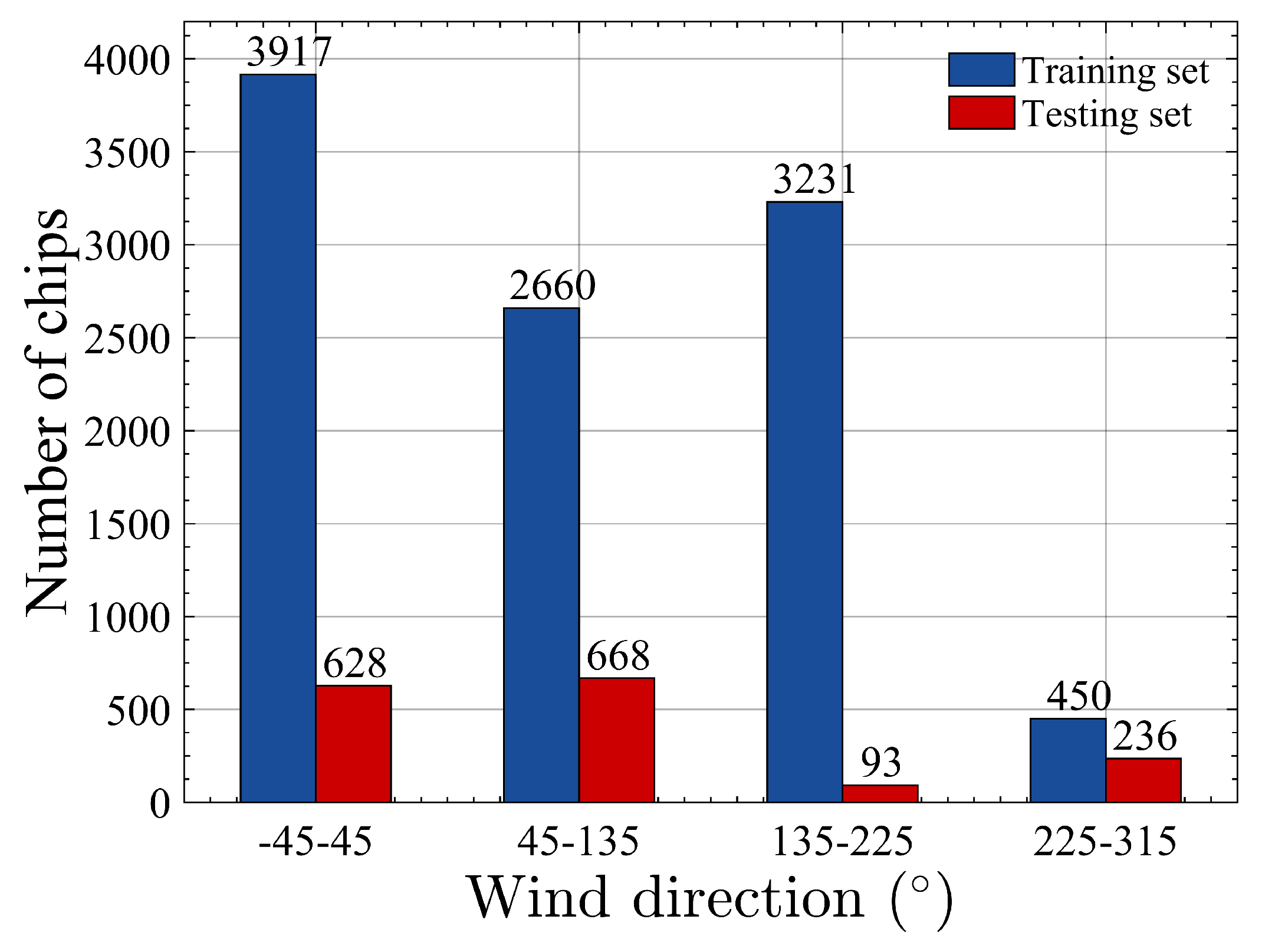
Figure 5.
Incidence angle histogram of the matchup dataset.
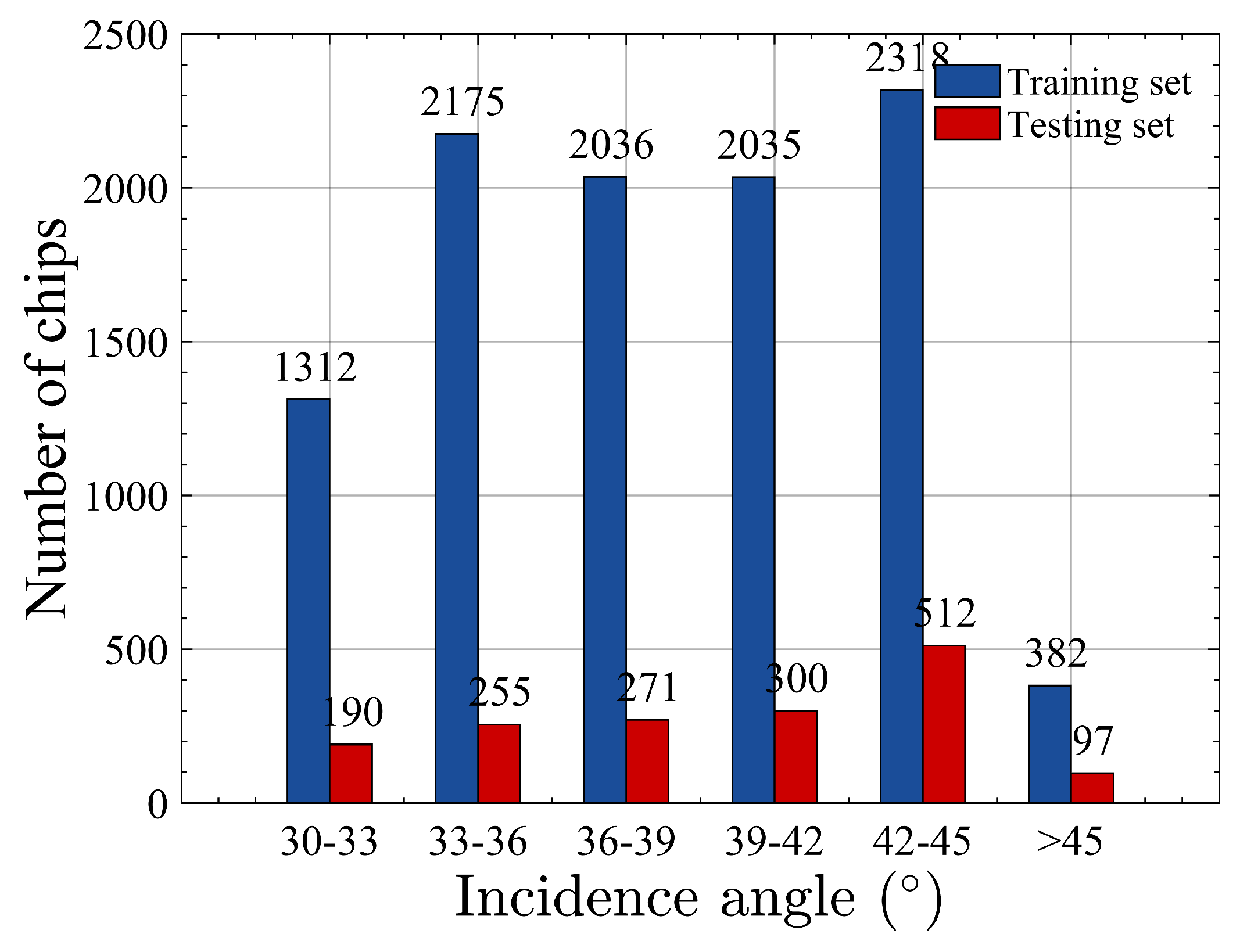
Figure 6.
Spatial distance error histogram of the matchup dataset.
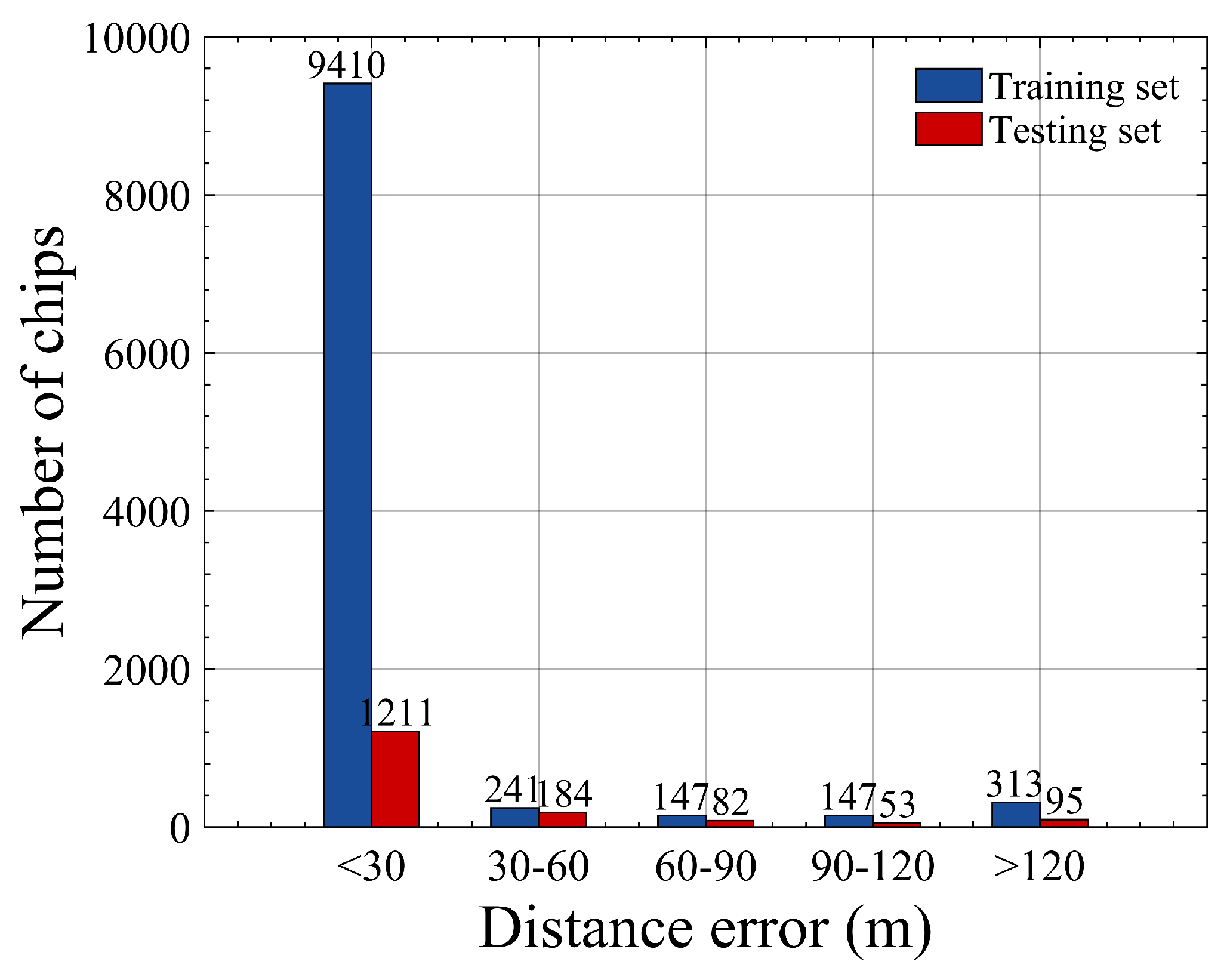
Figure 7.
Relationship between NRCS and incidence angle (different colors represent different wind speeds).
Figure 7.
Relationship between NRCS and incidence angle (different colors represent different wind speeds).

Figure 8.
Relationship between NRCS and incidence angle (different colors represent different wind directions).
Figure 8.
Relationship between NRCS and incidence angle (different colors represent different wind directions).

Figure 9.
Relationship between NRCS and wind speeds for IW1-band.

Figure 10.
Relationship between NRCS and wind speeds for IW2-band.
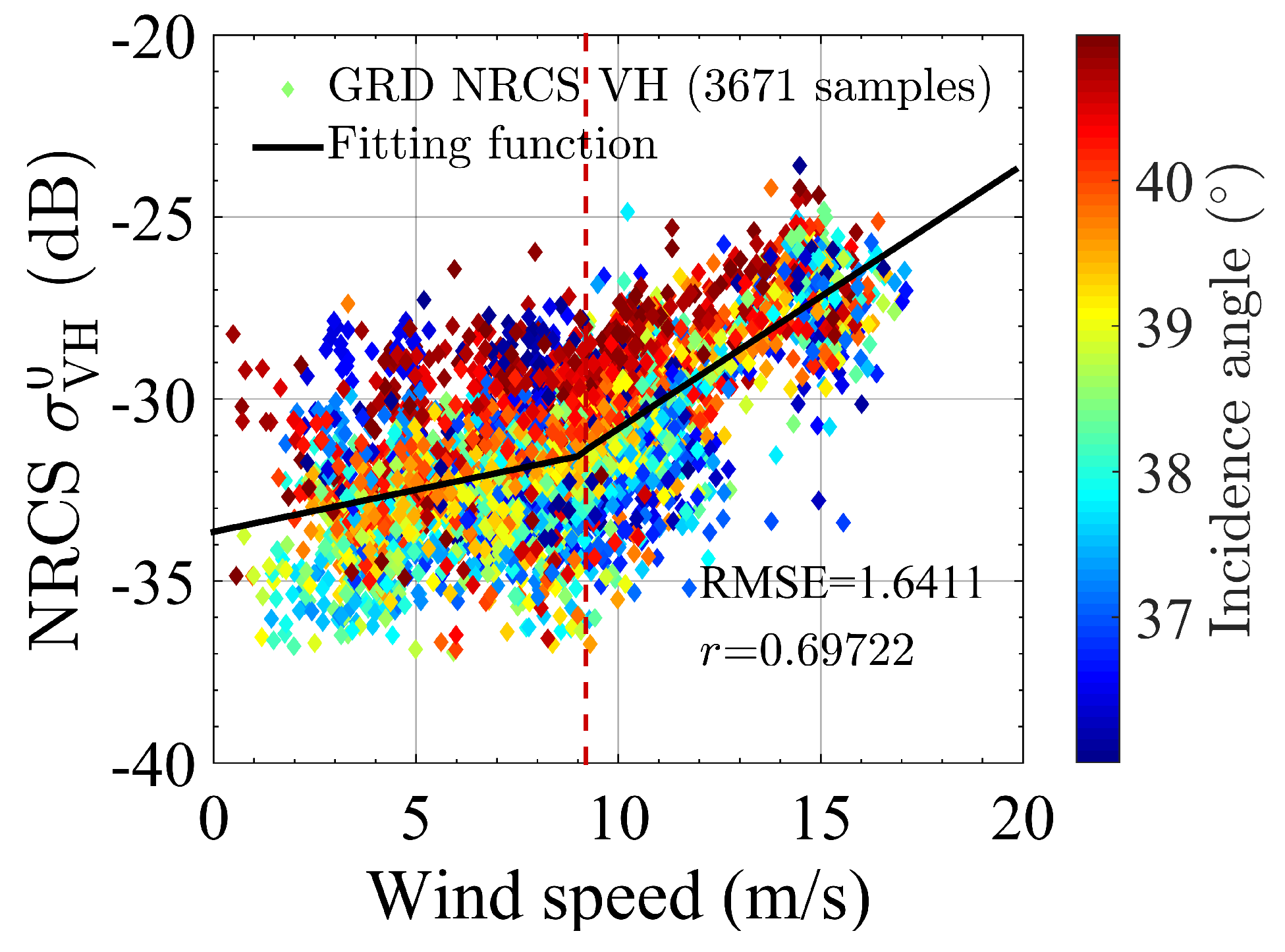
Figure 11.
Relationship between NRCS and wind speeds for IW3-band.

Figure 12.
Dependencies of the NRCS on wind direction. (a–f) show wind speed intervals of at 3, 5, 7, 9, 11, and , respectively. The red line represents the trendline.
Figure 12.
Dependencies of the NRCS on wind direction. (a–f) show wind speed intervals of at 3, 5, 7, 9, 11, and , respectively. The red line represents the trendline.

Figure 13.
Incidence angle function for IW1-band.

Figure 14.
Incidence angle function for IW2-band.

Figure 15.
Estimated NRCS of the proposed model for IW1-band.

Figure 16.
Estimated NRCS of the proposed model for IW2-band.
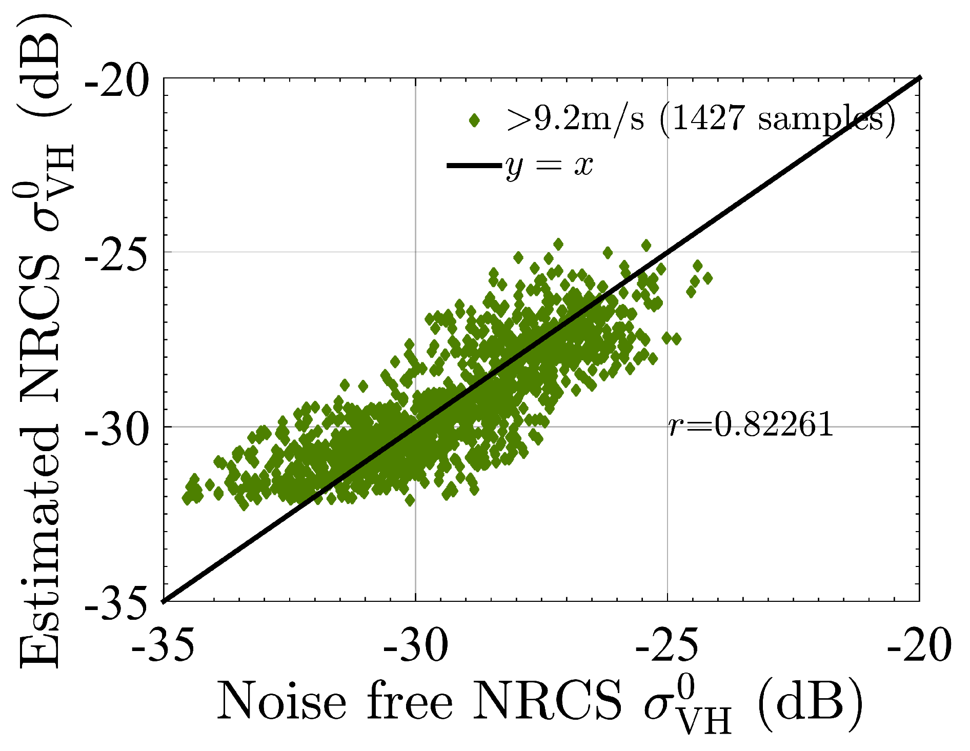
Figure 17.
Comparison of the estimated wind speed with ASCAT wind speed.

Table 1.
Parameters for Sentinel-1 IW GRD products [25].
Table 1.
Parameters for Sentinel-1 IW GRD products [25].
| Product Type | Resolution (rg × az) () | Pixel Spacing (rg × az) () | Swath Width (km) | Looks (rg × az) | Equivalent Number of Independent Looks |
|---|---|---|---|---|---|
| GRD | 250 | 4.9 |
Table 2.
Relationship of NRCS and wind speed for different sub-bands.
| Number of Samples | RMSE | r | Fitting Function | |
|---|---|---|---|---|
| IW1-band | 3487 | |||
| IW2-band | 3671 | |||
| IW3-band | 3100 |
Table 3.
Relationship of NRCS and wind direction.
| Direction | [] | [] | |||||
|---|---|---|---|---|---|---|---|
| NRCS (dB) | |||||||
| Speed | |||||||
| NaN | NaN | ||||||
Table 4.
Parameters for the proposed model.
| Incidence Angle | Wind Speed | C | ||
|---|---|---|---|---|
| IW1-band | 30– | 8–12.3 | ||
| IW1-band | 30– | > | ||
| IW2-band | 36– | > |
Table 5.
Performances of the proposed and compared model.
| Bias | RMSE | |||
|---|---|---|---|---|
| The proposed model | ||||
| The compared model |
Table 6.
Parameters of the model for datasets with different training and testing samples.
| Dataset | Incidence Angle | Wind Speed | Wind Speed Function | Incidence Angle Function | C | |
|---|---|---|---|---|---|---|
| 1 | 30– | 8–12.3 | ||||
| 30– | > | |||||
| 36– | > | |||||
| 2 | 30– | 8–12.3 | ||||
| 30– | > | |||||
| 36– | > | |||||
| 3 | 30– | 8–12.3 | ||||
| 30– | > | |||||
| 36– | > |
Table 7.
Performances of the model for datasets with different training and testing samples.
| Dataset | Bias | RMSE | ||
|---|---|---|---|---|
| 1 | ||||
| 2 | ||||
| 3 |
Table 8.
Parameters of the model for datasets with different number of pixels.
| Pixel Number | Incidence Angle | Wind Speed | Wind Speed Function | Incidence Angle Function | C | |
|---|---|---|---|---|---|---|
| 30– | 8–12.3 | |||||
| 30– | > | |||||
| 36– | > | |||||
| 30– | 8–12.3 | |||||
| 30– | > | |||||
| 36– | > | |||||
| 30– | 8–12.3 | |||||
| 30– | > | |||||
| 36– | > |
Table 9.
Performances of the model for datasets with different number of pixels.
| Pixel Number | Bias | RMSE | ||
|---|---|---|---|---|
© 2017 by the authors. Licensee MDPI, Basel, Switzerland. This article is an open access article distributed under the terms and conditions of the Creative Commons Attribution (CC BY) license (http://creativecommons.org/licenses/by/4.0/).
Share and Cite
MDPI and ACS Style
Huang, L.; Liu, B.; Li, X.; Zhang, Z.; Yu, W. Technical Evaluation of Sentinel-1 IW Mode Cross-Pol Radar Backscattering from the Ocean Surface in Moderate Wind Condition. Remote Sens. 2017, 9, 854. https://doi.org/10.3390/rs9080854
AMA Style
Huang L, Liu B, Li X, Zhang Z, Yu W. Technical Evaluation of Sentinel-1 IW Mode Cross-Pol Radar Backscattering from the Ocean Surface in Moderate Wind Condition. Remote Sensing. 2017; 9(8):854. https://doi.org/10.3390/rs9080854
Chicago/Turabian StyleHuang, Lanqing, Bin Liu, Xiaofeng Li, Zenghui Zhang, and Wenxian Yu. 2017. "Technical Evaluation of Sentinel-1 IW Mode Cross-Pol Radar Backscattering from the Ocean Surface in Moderate Wind Condition" Remote Sensing 9, no. 8: 854. https://doi.org/10.3390/rs9080854
Note that from the first issue of 2016, this journal uses article numbers instead of page numbers. See further details here.