Topic Modelling for Object-Based Unsupervised Classification of VHR Panchromatic Satellite Images Based on Multiscale Image Segmentation

Abstract

Image segmentation is a key prerequisite for object-based classification. However, it is often difficult, or even impossible, to determine a unique optimal segmentation scale due to the fact that various geo-objects, and even an identical geo-object, present at multiple scales in very high resolution (VHR) satellite images. To address this problem, this paper presents a novel unsupervised object-based classification for VHR panchromatic satellite images using multiple segmentations via the latent Dirichlet allocation (LDA) model. Firstly, multiple segmentation maps of the original satellite image are produced by means of a common multiscale segmentation technique. Then, the LDA model is utilized to learn the grayscale histogram distribution for each geo-object and the mixture distribution of geo-objects within each segment. Thirdly, the histogram distribution of each segment is compared with that of each geo-object using the Kullback-Leibler (KL) divergence measure, which is weighted with a constraint specified by the mixture distribution of geo-objects. Each segment is allocated a geo-object category label with the minimum KL divergence. Finally, the final classification map is achieved by integrating the multiple classification results at different scales. Extensive experimental evaluations are designed to compare the performance of our method with those of some state-of-the-art methods for three different types of images. The experimental results over three different types of VHR panchromatic satellite images demonstrate the proposed method is able to achieve scale-adaptive classification results, and improve the ability to differentiate the geo-objects with spectral overlap, such as water and grass, and water and shadow, in terms of both spatial consistency and semantic consistency.

1. Introduction

Recent advances in remote sensing technology, particularly those relating to spatial resolution, are helping to make detailed observations of the Earth’s surface possible. However, the resulting vast amounts of very high resolution (VHR) satellite images pose a challenge for automatic classification, due to the large amount of information and with-class variance characteristics of this kind of images [1].

It is widely acknowledged that, compared to their pixel-based counterparts, object-based classification methods, which can take advantage of both spectral and spatial information, are probably more appropriate for VHR satellite images [2,3,4]. In a typical object-based classification framework, image segmentation is usually an initial and vital step. The goal of segmentation is to partition an original image into a set of non-overlapping homogeneous segments, which are regarded as higher-level units that are more meaningful and efficient for subsequent processing. Thus, the classification accuracy of object-based classification is dependent, to a large extent, on the quality of image segmentation [5]. In order to characterize image structures at different scales, multiscale segmentation (MS) is often used to conduct a series of segmentation maps at multiple scales from fine to coarse ones, sequentially, by varying the scale parameter (SP) [6]. As pointed out by Dragut et al. [6], the SP controls the average segment size, i.e., a smaller value of the SP produces segmentations with small regions and detailed structures, and a larger value allows for more merges, thus preserving only large segments and coarse features. Therefore, the SP needs to be appropriately determined in order to create segments that can match the actual boundaries of landscape features of various sizes as much as possible [7]. However, there exist several problems in practical applications: (1) the determination of the optimal SP, in many cases, still relies on a trial-and-error optimization, which is time-consuming when it applies to complex image scenes [8]; (2) it is often impossible to determine a unique optimal SP for a whole scene or each geo-object, due to the fact that different geo-objects and even an identical geo-object may appear at different scales in the same image. Any specific SP is likely to cause over-segmentation of some parts of the image, but under-segmentation of other parts.

To overcome these shortcomings, many approaches that attempt to directly model multiple segmentations have been proposed instead of seeking and using an optimal one from multiple candidate segmentation maps [9,10,11,12]. In this direction, Russel et al. [10] used multiple segmentations to discover objects in natural image collections. The authors assumed while none of the SP settings can achieve the optimal image segmentation, some segments in some of the segmentations appear to be correct. Therefore, instead of selecting any particular optimal SP, they utilized multiple segmentation results to identify objects of various sizes by the learning machine. In a similar framework, Akcay et al. [13] proposed automatic detection of geospatial objects using multiple hierarchical segmentations. Afterwards, Santos et al. [14] presented a kind of boost-classifier adapted to MS for supervised classification, in which a sequential strategy of training for weak classifiers was adopted based on a hierarchy of image segmentations from fine to coarse. However, both [13] and [14] are built on hierarchical image segmentation [15], which cannot be directly obtained in many cases due to the reason that most image segmentation methods do not consider the hierarchical structures. These observations motive us to develop a novel object-based unsupervised classification based on MS, in which multiple segmentation maps are jointly utilized by means of topic modelling. In the proposed framework, the original image does not require to be hierarchically partitioned to form multiple segmentation maps.

Attracted by the success of topic models, e.g., latent Dirichlet allocation (LDA) [16] and its relatives [17,18], in text analysis community, there has been an increasing interest in applying such models for semantically-driven understanding of satellite images, such as image annotation [19,20,21], object detection [13,22], scene classification [23,24,25], and image classification or clustering [26,27,28,29]. Among various advantages provided by topic models is their ability to deal with polysemy [16]. For example, the word “bachelor” could refer to a kind of degree or an unmarried man. Based on co-occurrence of words in the context, topic models are able to capture the polysemous use of words. This characteristic offers a potential solution to cope with the perplexing, but so common, phenomenon in VHR satellite image classification, i.e., different geo-objects with nearly identical spectra. For image classification or clustering, the square image blocks with fixed-size or segments with arbitrary shape are viewed as the documents [27,29], and the pixels or local patches extracted from the images are regarded as the words in topic modeling. Using the probabilistic latent semantic analysis (pLSA) model, Yi et al. [26] presented a novel semantic clustering algorithm for VHR satellite images. The experiment results confirmed the advantage of topic modelling. However, in the proposed framework, a pre-processing step was required to partition the original satellite image into image documents, and an accompanying post-processing step was required to combine the allocated multiple labels of a pixel into a unique one using a certain voting rule. To address this problem, Tang et al. [27] developed a msLDA model, which built an automatic framework that combined a latent Dirichlet allocation with a multiscale image representation of a panchromatic satellite image. The msLDA archived an adaptive smoothing on clustering results. Nevertheless, its application usually introduces a computational bottleneck, due to the manner in which image documents are generated, where each pixel and its surrounding pixels within the square neighborhood constitute a document. Shu et al. [30] presented a nonparametric Bayesian hierarchical model to conduct unsupervised classification of VHR panchromatic satellite images by considering over-segments as documents. However, it also suffers from the same problems as the traditional object-based methods mentioned previously, i.e., it is modelled based on single-scale segmentation.

In this paper, a novel object-based unsupervised classification for VHR panchromatic satellite images using multiple image segmentation maps via the LDA model is presented. The proposed approach consists of four components: (1) a multiscale image segmentation component that allows characterizing of image structures at different scales; (2) a topic model component that learns the grayscale histogram distribution for each geo-object and the mixture distribution of geo-objects in each segment in an unsupervised manner; (3) a category label allocation component that classifies each segment by the ranking of probability-based similarities; and (4) an automatic application framework component that integrates multiple classification results at different scales into a unique one. It should be noted that while the proposed method still needs to determine the range of scales for creating a multiscale segmentation representation, the work has been greatly simplified compared to searching for the optimal image segmentation. The main contribution of the proposed method is an automatic framework of combining a topic model with a multiscale image segmentation representation to model both the co-occurrence of various geo-objects and multiscale structures.

This paper extends and improves on a preliminary work [31], which presents our initial ideas and results. In this paper: (1) a novel strategy of integrating multiple classification results at different scales into a unique one is added, which can ensure an adaptive smoothing classification result can be achieved; (2) a constraint specified by the mixture distribution of geo-objects, which can characterize the co-occurrence relationships of various geo-objects, is incorporated to correct the KL similarity between the histogram distribution of each segment and that of each geo-object; and (3) a more thorough presentation of introduction, methodology, experimental analysis, and discussion is conducted.

The remainder of this paper is organized as follows. In Section 2, the proposed methodology is presented in detail. Experimental results and related discussion are given in Section 3. Finally, the conclusion is drawn in Section 4.

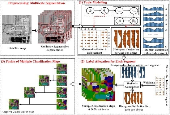
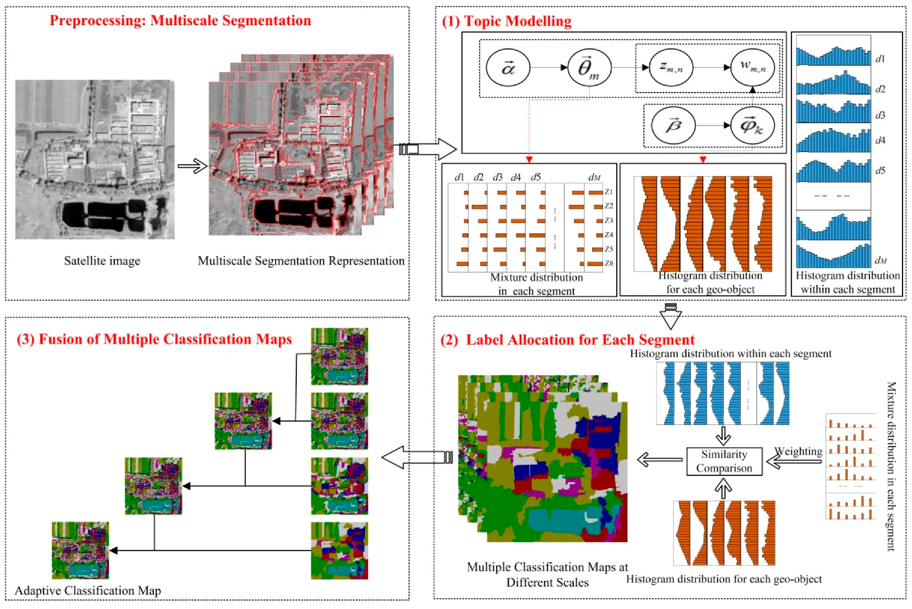
2. Methodology

In this section, we present our approach for performing the object-based unsupervised classification of panchromatic satellite images, using the LDA model.

For the proposed method, a key prerequisite is to create a MS representation of the original satellite image with varied scales. Since the goal of MS is to produce enough segmentation maps of the image so as to have a high probability of acquiring better segments that can correspond to potential geo-objects, we do not need image segmentation at each scale to be exactly correct. Any method that can create a reasonable MS of a satellite image may meet the requirement.

Given the MS representation, the proposed method is composed of the following three steps: Firstly, the LDA model is utilized to learn the grayscale histogram distribution for each geo-object and the mixture distribution of geo-objects within each segment in an unsupervised manner. Then, the histogram distribution of each segment is compared with that of each geo-object using the Kullback-Leibler (KL) divergence measure [10], which is further weighted with a constraint specified by the mixture distribution of geo-objects. Each segment is allocated a geo-object category label with the minimum KL divergence. Finally, the scale-adaptive unsupervised classification map is achieved by integrating the multiple classification results at different scales. The general scheme is shown in Figure 1.

2.1. Topic Modelling

2.1.1. Latent Dirichlet Allocation

The LDA is a generative hierarchical Bayesian probabilistic model, which is originally proposed to model collections of discrete data, such as text documents and natural images [32]. In this model, each document is viewed as a finite mixture of various latent topics. Each topic, in turn, is a probability distribution over words. For a corpus of M documents, the LDA assumes the following generative process for the m-th document of length N:

• For the k-th element of K topics, sample the topic-specific term distribution ${\overrightarrow{\varphi }}_k$ according to the Dirichlet distribution, i.e., ${\overrightarrow{\varphi }}_k\sim \mathrm{Dirchlet}(\overrightarrow{\beta })$, where $\overrightarrow{\beta }$ is the hyperparameter.
• Sample the topic mixture ${\overrightarrow{\theta }}_m$ according to the Dirichlet distribution, i.e., ${\overrightarrow{\theta }}_m\sim \mathrm{Dirchlet}(\overrightarrow{\alpha })$, where $\overrightarrow{\alpha }$ is the hyperparameter.
• For each word $w_{mn}\in \{w_{m1},w_{m2},\dots ,w_{mN}\}$, sample a topic $z_{mn}$ according to the multinomial distribution, i.e., $z_{mn}\sim \mathrm{Multinomial}({\overrightarrow{\theta }}_m)$, and sample a word $w_{mn}$ according to the multinomial distribution , i.e., $w_{mn}\sim \mathrm{Multinomial}({\overrightarrow{\varphi }}_{z_{mn}})$.

Both variational inference and Gibbs sampling have been used to infer and estimate the parameters of the LDA. To solve the inferential problem, we need to calculate the posterior probability of the hidden variables given a corpus, i.e., $P(\overrightarrow{z}|\overrightarrow{w},\overrightarrow{\alpha },\overrightarrow{\beta })$. The general formulation of a Gibbs sampler for such latent-variable models becomes:

$$P(z_i|{\overrightarrow{z}}_{-i},\overrightarrow{w},\overrightarrow{\alpha },\overrightarrow{\beta })=\frac{P(\overrightarrow{z},\overrightarrow{w}|\overrightarrow{\alpha },\overrightarrow{\beta })}{{\displaystyle \underset{Z}{\int }P(\overrightarrow{z},\overrightarrow{w}|\overrightarrow{\alpha },\overrightarrow{\beta })d{z}_i}},$$

(1)

which can be approximated by interactively sampling each of the K topics using the chain rule and noting that $\overrightarrow{w}=\{{\overrightarrow{w}}_{-i},w_i=v\}$ and $\overrightarrow{z}=\{{\overrightarrow{z}}_{-i},z_i=k\}$:

$$\begin{array}{l}P(z_i|{\overrightarrow{z}}_{-i},\overrightarrow{w},\overrightarrow{\alpha },\overrightarrow{\beta })=\frac{P(\overrightarrow{z},\overrightarrow{w}|\overrightarrow{\alpha },\overrightarrow{\beta })}{P({\overrightarrow{z}}_{-i},\overrightarrow{w}|\overrightarrow{\alpha },\overrightarrow{\beta })}\\ \propto \frac{n_{k,-i}^{(v)}+{\beta }_t}{{\displaystyle \sum _{v^{\prime }=1}^V(n_k^{(v^{\prime })}}+{\beta }_{v^{\prime }})-1}*\frac{n_{m,-i}^{(k)}+{\alpha }_k}{{\displaystyle \sum _{k^{\prime }=1}^K(n_m^{(k^{\prime })}}+{\alpha }_{k^{\prime }})}\end{array},$$

(2)

where the counts $n_{.,-i}^{(.)}$ represents the number of the words or topics with exception of index $i$.

For a new topic-word pair $(\tilde{z}=k,\tilde{w}=v)$ that is observed in a document $d(\tilde{w})=d(\tilde{z})=m$, given the state $(\tilde{z},\tilde{w})$, the multinomial parameters can be determined by:

$${\varphi }_{k,v}=\frac{n_k^{(v)}+{\beta }_v}{{\displaystyle \sum _{v^{\prime }=1}^V(n_k^{(v^{\prime })}}+{\beta }_{v^{\prime }})},$$

(3)

$${\theta }_{m,k}=\frac{n_m^{(k)}+{\alpha }_k}{{\displaystyle \sum _{k^{\prime }=1}^K(n_m^{(k^{\prime })}}+{\alpha }_{k^{\prime }})},$$

(4)

where $V$ is the number of words in the vocabulary, ${\alpha }_k$ and ${\beta }_v$ stand for the k-th element and v-th element of hyperparameter $\overrightarrow{\alpha }$ and $\overrightarrow{\beta }$, respectively. For details regarding the derivation, please refer to [33].

2.1.2. Build an Analogue of Text-Related Terms in the Image Domain

To borrow techniques used in the text domain to satellite images, the first issue that needs to be addressed is how to build an analogue of text terms in the image domain. For the proposed method, we follow the definition in [27,29]

• Word: a unique grayscale value of a pixel is defined as a word;
• Vocabulary: the unique grayscale values of the satellite image form the vocabulary;
• Document: each segment is regarded as a document, thus, all segments of multiple segmentation maps at different scales constitute the corpus;
• Topic: each topic corresponds to a specific geo-object category.

Given multiple segmentation maps at different scales, we can use the LDA model to learn K grayscale histogram distributions for K geo-objects, i.e., ${\{{\overrightarrow{\varphi }}_k\}}_{k=1}^K$, and M mixture distributions of geo-objects within M segments, i.e., ${\{{\overrightarrow{\theta }}_m\}}_{m=1}^M$. Furthermore, M grayscale histogram distributions within M segments, i.e., ${\left\{{\overrightarrow{\pi }}_m\right\}}_{m=1}^M$, can also be easily obtained just by counting the frequencies of different grayscale values.

2.2. Label Allocation for Each Segment

Although there may be some differences in size due to the scale effect, the segments that correspond to the identical geo-object should have similar grayscale histogram distributions. As a consequence, the category label allocation for each segment is determined according to the following rule: the histogram distribution of each segment is compared with those of K geo-objects, respectively. The similarity between two types of distributions is measured using the KL divergence, which has been proved to be effective in measuring the probability-based similarity. The category label of the geo-object, which has the minimum KL divergence with the segment, is allocated as the label of the segment. Given the segment $d_m$, its category label $c_{d_m}$ is mathematically given by:

$$c_{d_m}=\arg \underset{1\le k\le K}{\min }KL({\overrightarrow{\pi }}_m,{\overrightarrow{\varphi }}_k),$$

(5)

where $KL({\overrightarrow{\pi }}_m,{\overrightarrow{\varphi }}_k)$ denotes the symmetrical KL divergence between two discrete distributions, i.e., ${\overrightarrow{\pi }}_m$ and ${\overrightarrow{\varphi }}_k$. To be specific, the symmetrical KL divergence in the discrete form can be represented as the following:

$$KL({\overrightarrow{\pi }}_m,{\overrightarrow{\varphi }}_k)=\frac{{\displaystyle \sum _{v=1}^V\{{\pi }_m^{v}In(\frac{{\pi }_m^v}{{\varphi }_k^v})+{\varphi }_k^{v}In(\frac{{\varphi }_k^v}{{\pi }_m^v})\}}}{2},$$

(6)

where ${\pi }_m^v$ refers to the v-th element of ${\overrightarrow{\pi }}_m$, which describes the histogram distribution within the segment m. Likewise, ${\varphi }_k^v$ refers to the v-th element of ${\overrightarrow{\varphi }}_k$, which describes the histogram distribution for the geo-object k.

Furthermore, it is easy to understand: with the increase of the mixture proportion of a certain geo-object within the segment, the probability of classifying the segment as the corresponding geo-object should be improved accordingly. The mixture distribution of geo-objects within each segment, i.e., ${\{{\overrightarrow{\theta }}_m\}}_{m=1}^M$, learned by topic modelling, exactly provides the mixture proportion features. Thus, Equation (5) can be further weighted with a constraint specified by the mixture distribution of geo-objects:

$$c_{d_m}=\arg \underset{1\le k\le K}{\min }KL({\overrightarrow{\pi }}_m,{\overrightarrow{\varphi }}_k)\cdot u_m^k,$$

(7)

where ${\overrightarrow{u}}_m$ is empirically set to $-In({\overrightarrow{\theta }}_m)$, and $u_m^k$ denotes the weight with the geo-object k.

Overall, by means of Equation (7), the category label of each segment is determined jointly by both the grayscale distribution and mixture distribution of geo-objects, which can characterize the co-occurrence relationships of various geo-objects.

2.3. Fusion of Multiple Classification Maps

After finishing step 2.2, multiple unsupervised classification maps at different scales are achieved. However, due to the existence of multiscale effects in VHR satellite images, any classification map based the single-scale segmentation cannot take into account the various granularities of the geo-objects, e.g., the narrow roads may be suitable to be extracted at a fine scale, while the large-area field should be classified at a coarse scale. Therefore, the final classification map is achieved by integrating the multiple classification maps at different scales, in order to achieve a scale-adaptive unsupervised classification.

Given the scale range $\{1,2,\dots ,S\}$, $S$ classification maps at multiple scales can be obtained by the means of topic modelling presented above. In other words, each pixel i in the original satellite image will be allocated $S$ category labels. Let $d_{i,s}$($s\in \{1,2,\dots S\}$) denote the segment covering the pixel i at the scale s, and $k(d_{i,s})$ denote the category label of the segment $d_{i,s}$, the category label of the pixel i is given by:

$$\{\begin{array}{l}{s}^{*}=\arg \underset{1\le s\le S}{\min }KL({\overrightarrow{\pi }}_{d_{i,s}},{\overrightarrow{\varphi }}_{k(d_{i,s})}),\\ c_i=k(d_{i,s^{*}}).\end{array},$$

(8)

where ${\overrightarrow{\pi }}_{d_{i,s}}$ denotes the grayscale histogram distribution within the segment $d_{i,s}$, ${\overrightarrow{\varphi }}_{k(d_{i,s})}$ denotes the grayscale histogram distribution for the geo-object $k(d_{i,s})$, and $s^{*}$ denotes the optimal scale for the pixel i.

3. Results and Discussion

In this section, we firstly describe the experimental images. Then, we introduce the quantitative evaluation methods for the experimental results and the state-of-art methods for comparison, and the parameter settings are also given in detail. Thirdly, we compare the performance of different approaches for three typical of geographical scenes in terms of both qualitative and quantitative aspects. The computational efficiency for different approaches is also discussed. Finally, we analyze the effects of scale setting in the proposed method on the classification results.

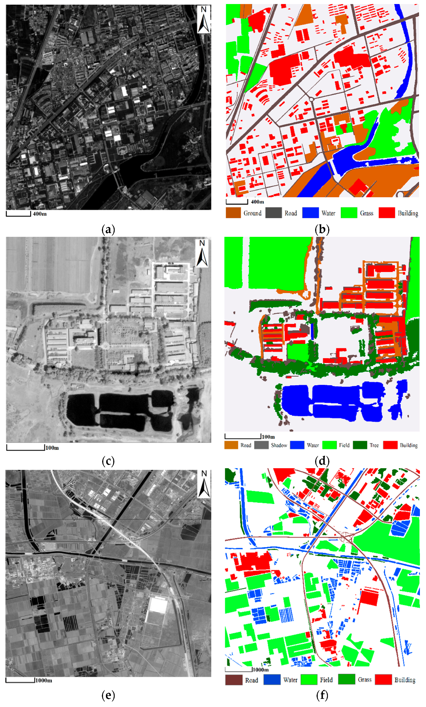
3.1. Experiment Data

In order to assess the effectiveness of the proposed approach, three panchromatic satellite images with different scenes and spatial resolutions are used. The first data is a panchromatic Mapping Satellite-1 image with 1600 × 1600 pixels and 2 m spatial resolution, which was acquired on 13 August 2012 and covers an area of Miyun District, Beijing, China. As shown in Figure 2a, five major types of geo-objects, i.e., building, road, water, grass, and ground, occur in this image. The second data is a panchromatic QuickBird image with 900 × 900 pixels and 0.6 m spatial resolution, as shown in Figure 2c. It was acquired on 22 April 2006 and located in Tong Zhou district of Beijing, China. There are six major types of geo-objects distributed in the image, including building, road, water, shadow, tree, and field. The third data is a panchromatic ZiYuan-3 (ZY-3) image that was acquired over an area of Tanggu District, Tianjin, China, on 15 August 2015. The image size is 3500 × 3500 pixels, and the spatial resolution is 2.1 m. As shown in Figure 2e, the image is made up of five major types of geo-objects, including building, road, water, grass, and field. We manually annotated all the original images at the pixel level as ground truth label data through visual interpretation. The corresponding ground truth maps for three satellite images are shown in Figure 2b,d,f, respectively.

3.2. Experiment Setup

3.2.1. Methods for Comparison with the Proposed Approach

To evaluate the effectiveness on three aspects of classification accuracy, spatial smoothness, and semantic consistency, the performance of the proposed approach is compared with that of four state-of-the-art unsupervised classification methods based on image segmentation: (1) the spectral-spatial ISODATA, where the pixel-based ISODATA classification is followed by a majority voting within the adaptive neighborhoods defined by the over-segmentation (termed as O_ISODATA) [34]; (2) the spectral-spatial LDA, similar to O_ISODATA, where the same over-segmentation is applied to the classification result of the LDA model using just the single-scale image segmentation map as corpus [30] (termed as O_LDA); (3) the msLDA proposed in [27]; and (4) the HDP_IBP proposed in [30].

For convenience, the proposed approach is referred to as the mSegLDA.

3.2.2. Evaluation Criteria

In our experiments, two quantitative criteria, as well as visual inspection, are utilized to evaluate the unsupervised classification results, i.e., overall accuracy (OA) and overall entropy (OE).

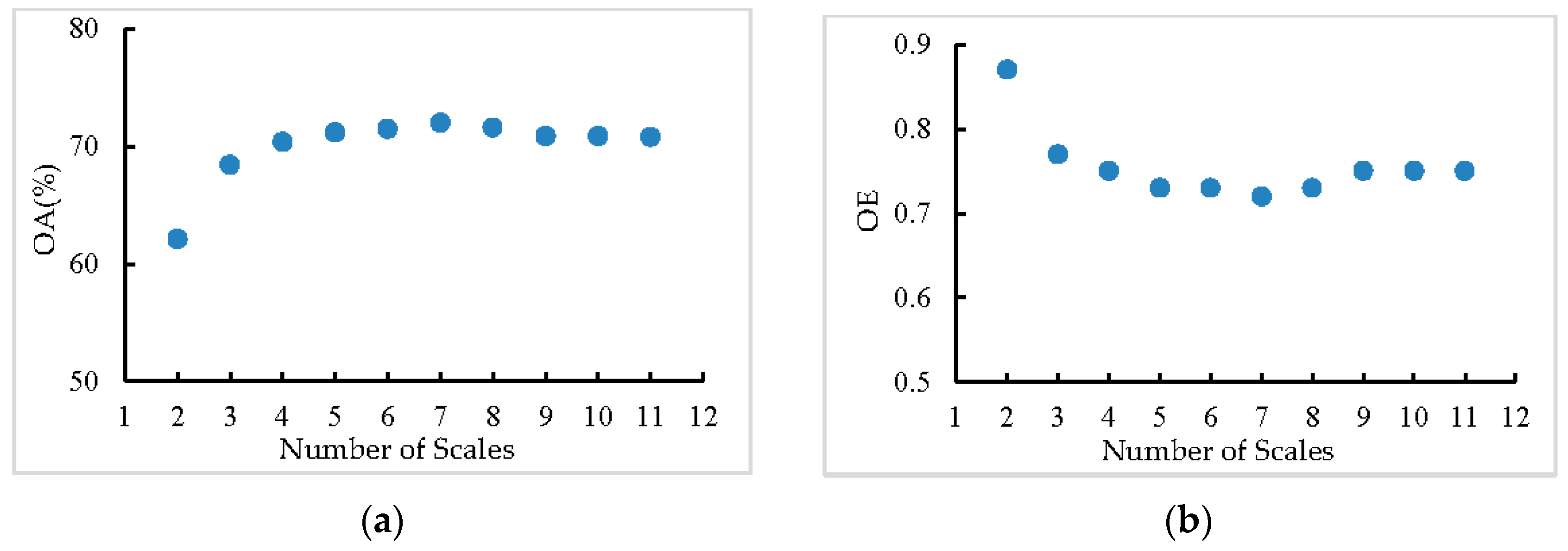
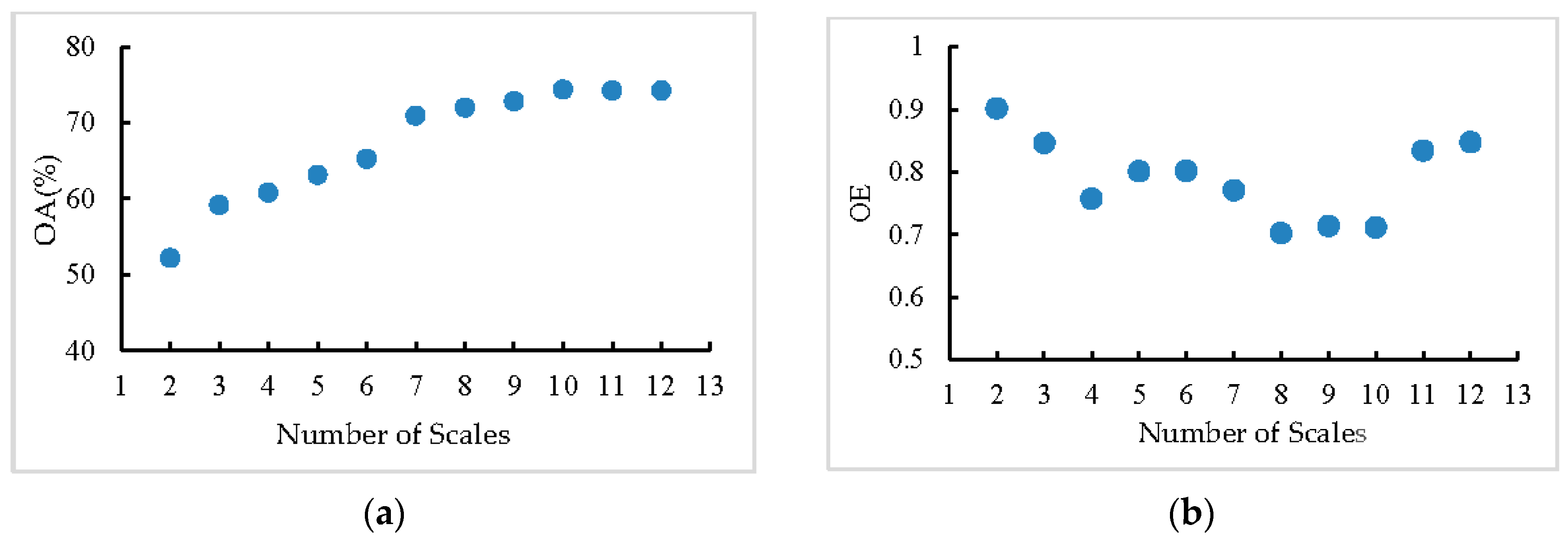
• Overall accuracy (OA): OA, which serves as a quantitative measurement of the agreement between the classification result and the ground truth map, is one of the most widely used statistics for evaluating the classification accuracy. OA can be calculated by dividing the total correctly-classified pixels by the total number of pixels checked by the ground truth map, and is given as $OA=N_{correct}/N_{total}$, where $N_{correct}$ is the total number of correct pixels, and $N_{total}$ is total number of pixels.
• Overall entropy (OE): entropy is an information theoretical criterion that is able to measure the homogeneity of the classification results. OE is defined as a linear combination of the class entropy, which describes how the pixels of the same geo-object are presented by the various clusters created, and the cluster entropy, which reflects the quality of the individual clusters in terms of the homogeneity of the pixels in a cluster. Generally speaking, a smaller overall entropy value corresponds to the classification map with a higher homogeneity. For details regarding, please refer to [27,35].

3.2.3. Parameter Setting

In order to produce multiple segmentation maps at different scales, this paper uses the entropy rate superpixel segmentation (ERSS) algorithm [36], which has been proven to be both effective and efficient. It should be noted that any method that can create a reasonable MS of satellite image may meet the requirement of the proposed approach. The ERSS algorithm utilizes the number of segments to control the scale size of image segmentation, i.e., a large number of segments may result in fine-scale segmentation, and conversely, a small number of segments will generate coarse-scale segmentation. For the Mapping Satellite-1 image, the QuickBird image and the ZY-3 image, the number of scales S is set to 6, 9, and 11, respectively, and the corresponding numbers of segments include {100, 200, 500, 800, 1000, 1500}, {100, 200, 500, 800, 1000, 1500, 2000, 2500, 3000}, and {2000, 3500, 5000, 6500, 8000, 9500, 11,000, 12,500, 14,000, 15,500, 17,000}.The range of scales, reflected by the numbers of segments, should be able to characterize multiscale structures in the images as much as possible. For both O_ISODATA and O_LDA, the over-segmentation map with 1500 segments, 2500 segments, and 17,000 segments are used in the three images.

Furthermore, topic model based methods initializes the Dirichlet priors as symmetric priors empirically, i.e., $\alpha =0.1$, $\beta =0.01$ for the Mapping Satellite-1 image, $\alpha =0.01$, $\beta =0.8$ for the QuickBird image, and $\alpha =50/K$, $\beta =0.01$ for the ZY-3 image. The number of geo-objects K is set to 6, 7, and 6 according to the distributions of geo-object classes, respectively.

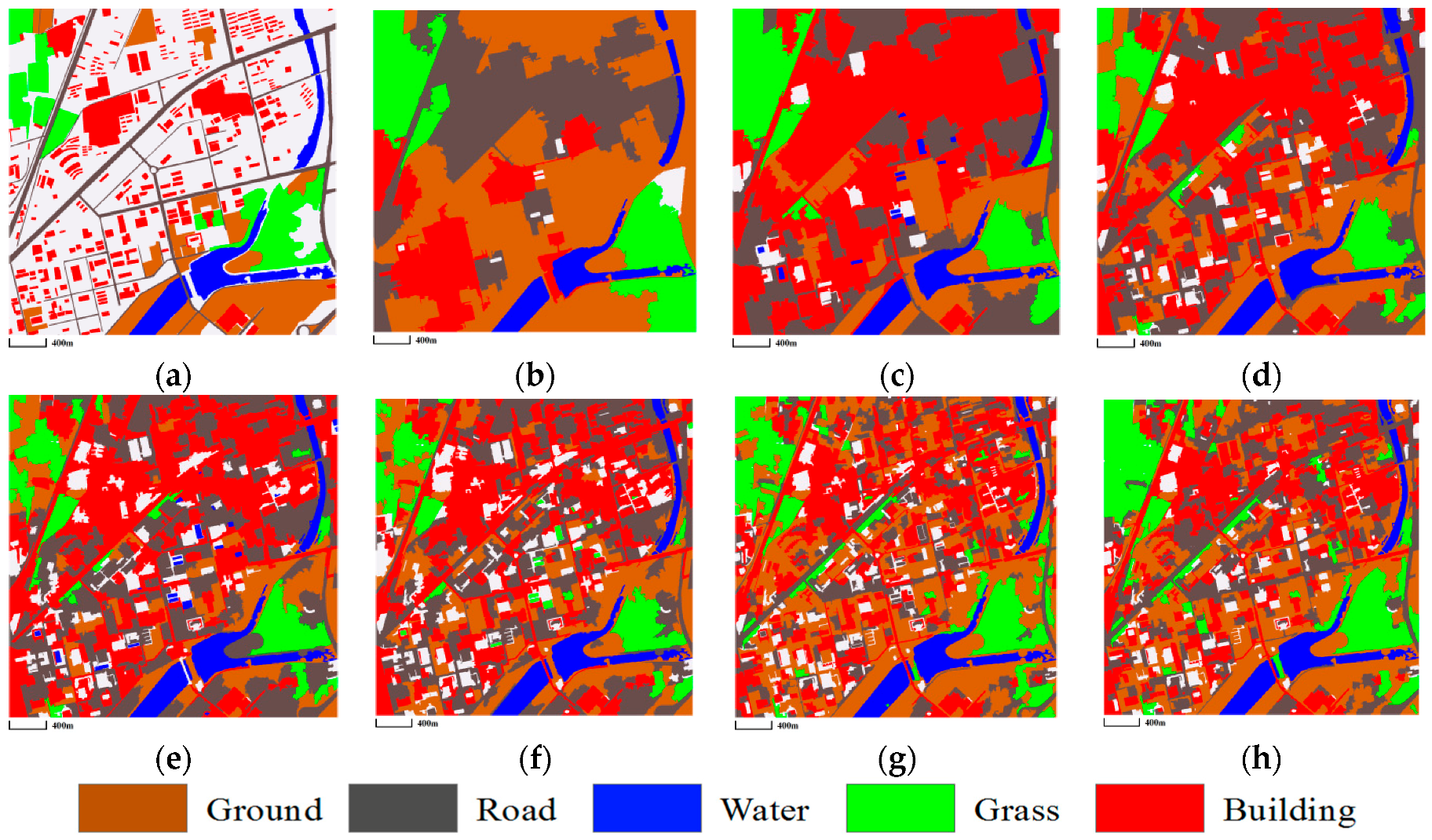
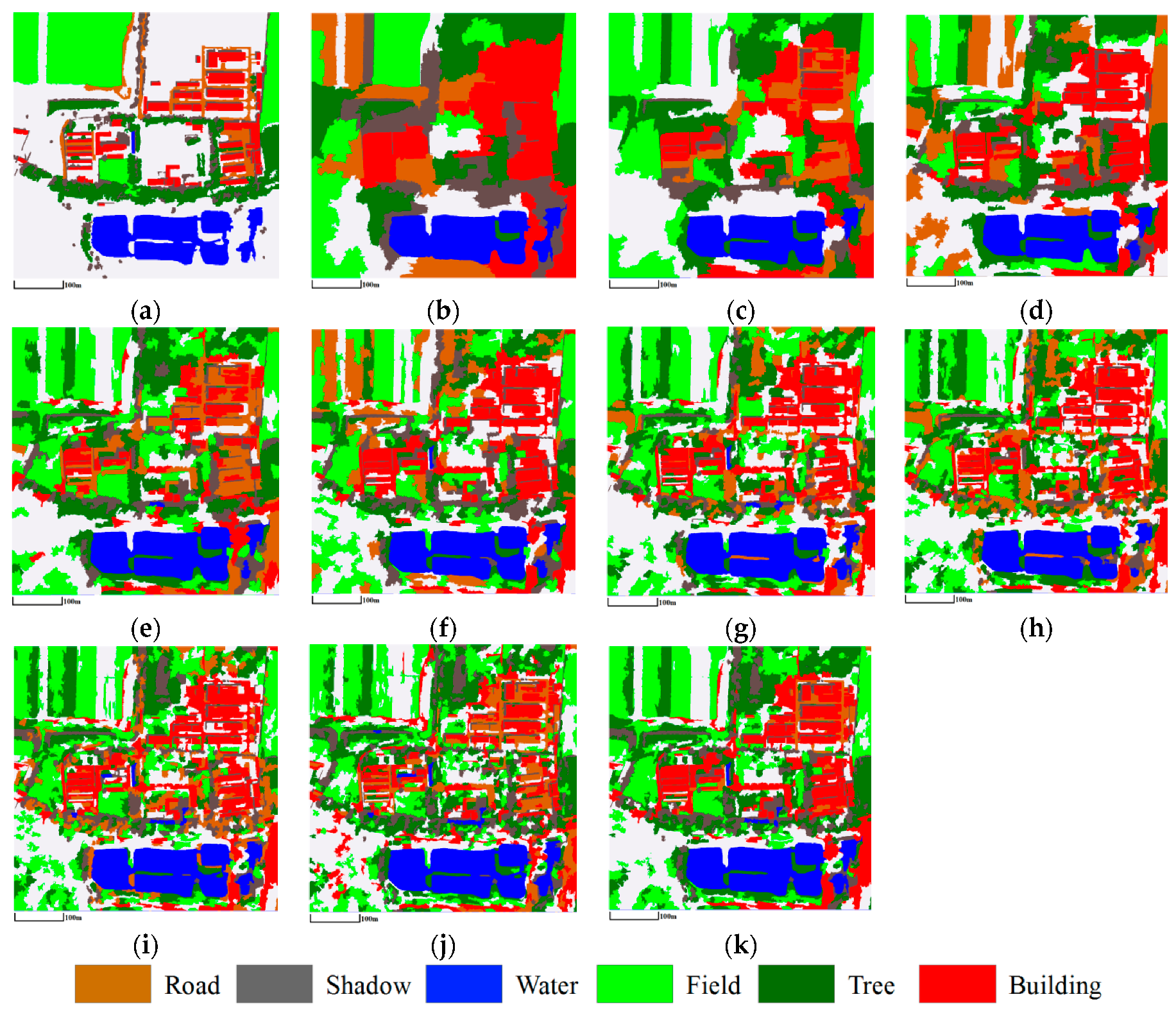
3.3. Comparison of Classification Results

The classification results of various methods for three satellite images are shown in Figure 3, Figure 4 and Figure 5, where each geo-object is represented by a different color.

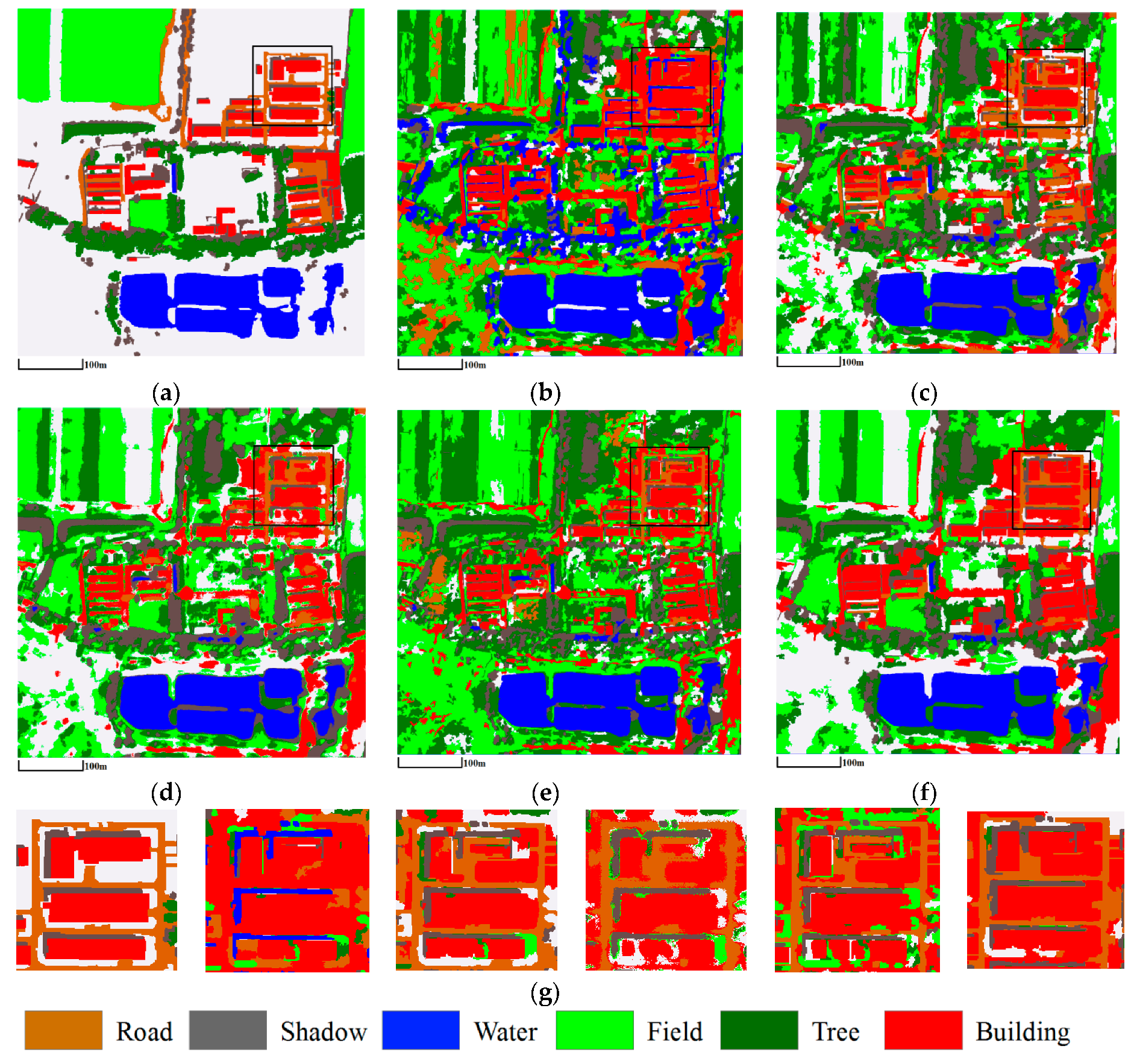
3.3.1. Mapping Satellite-1 and QuickBird Images

From visual inspection, all the unsupervised classification results seem to be compact. The obvious speckle noise or the isolated pixel patches which are often found in the results of pixel-based classification approaches are greatly eliminated. Thus, the advantages of enforcing spatial consistency over the classification by means of performing image segmentation are confirmed. On the other hand, obvious misclassification between water and grass in Figure 3b,g, and water and shadow in Figure 4b,g can be observed in the classification results of the ISODATA. Two types of geo-objects, i.e., grass and shadow, are entirely incorrectly identified as water. This phenomenon can be explained by the fact that there exist obvious spectral overlaps between water and grass in Figure 2a, and water and shadow in Figure 2c. For this reason, the ISODATA which groups image pixels merely according to their grayscale values and, thus, are not able to differentiate various geo-objects with similar spectra well. While the O_ISODATA that conducts pixel-based ISODATA classification, followed by spatial regularization using the segmentation map can ensure spatial continuity within segments, it does not change the essential mechanism of the ISODATA.

However, benefitting from topic modelling, for the topic model-based approaches, the co-occurrence information, characterized by the mixture distribution of various geo-objects within each segment, can be utilized to correctly recognize different objects with similar spectra. As illustrated in Figure 3c–g and Figure 4c–g, two types of geo-objects, i.e., grass and shadow, are well separated from water in the classification results of the topic model based approaches.

Furthermore, because the O_LDA is built on a single-scale over-segmentation map, it lacks a mechanism to model multiscale features of various-objects and, thus, cannot realize an adaptive smoothing on classification results. As shown in Figure 4c, the smoothing effect on the fine-scale road is proper, but is not sufficient for the large-scale field. Additionally, the majority voting scheme adopted by the O_LDA within the adaptive neighborhoods defined by the over-segmentation also results in the relatively fragmented classification map. In order to encode the scale-adaptive classification ability, the msLDA combines the topic model with a multiscale image representation derived by convoluting a given image with a variable-scale Gaussian into an automatic framework by embedding both image block and scale selections, and the HDP_IBP introduces the hierarchical spatial information, particularly the high-level scene cues, into the classification. As shown in Figure 3d–e and Figure 4d–e, both the HDP_IBP and msLDA improve the adaptive smoothing effect on the classification results to a certain extent compared with the O_LDA. However, the improvement is still limited. As a contrast, as shown in Figure 3f,g and Figure 4f,g the proposed mSegLDA could realized a more significant self-adaptive spatial regularization on classification results according to various geo-object types at different scales, i.e., the large-scale geo-object (e.g., field) is heavily smoothed, resulting in a more homogenous classification, and the fine-scale geo-object (e.g., road) accepts a slight smoothing, thus preserving detailed structures and edge patterns.

From quantitative evaluation, both OA and OE in different classification results for two experiment images are calculated, as shown in

Table 1. OA and OE of various methods for the Mapping Satellite-1 image.

	O_ISODATA	O_LDA	msLDA	HDP_IBP	mSegLDA
OA	48.6	69.3	68.4	70.1	72.0
OE	0.89	0.79	0.84	0.76	0.72

and

Table 2. OA and OE of various methods for the QuickBird image.

	O_ISODATA	O_LDA	msLDA	HDP_IBP	mSegLDA
OA	49.8	65.1	68.2	65.5	74.3
OE	0.96	0.84	0.80	0.84	0.71

, respectively. The mSegLDA approach yields the best classification accuracies and the lowest values of OE, compared to other methods, indicating the proposed method can achieve a better classification performance on the whole.

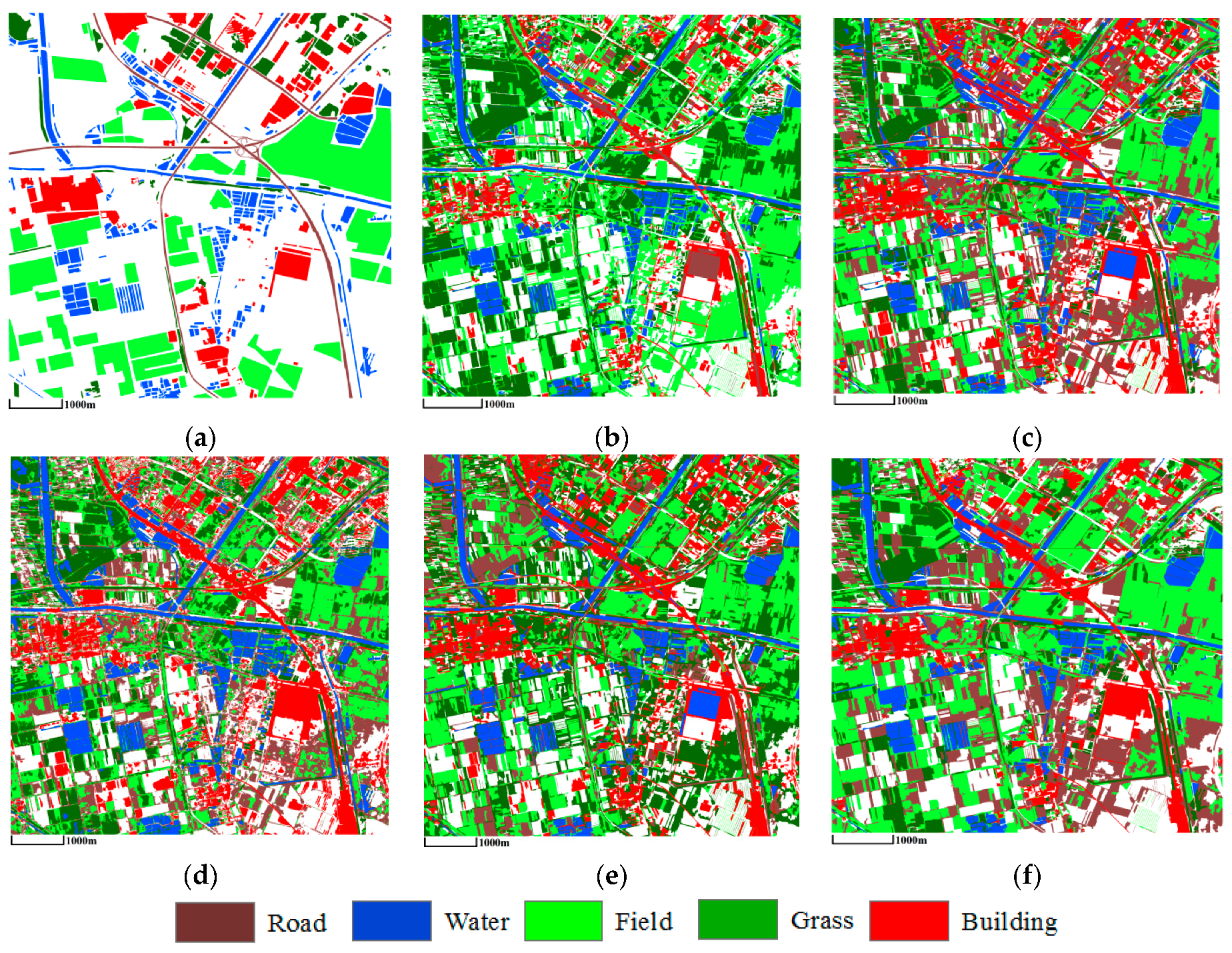
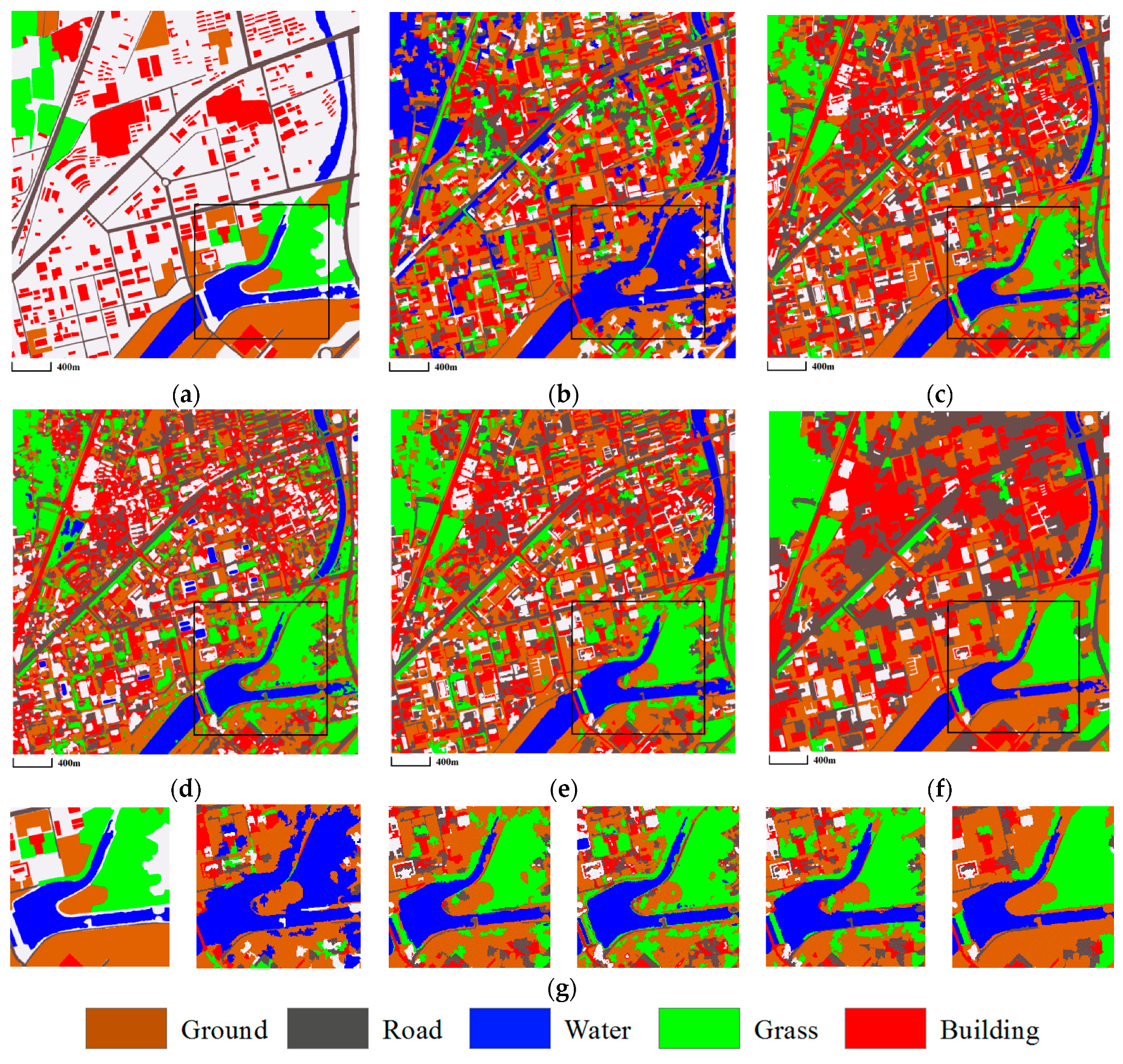
3.3.2. ZY-3 Image

In this subsection, a ZY-3 satellite image of a large scene covering over 50 km² is used to evaluate the effectiveness of the proposed mSegLDA. As shown in Figure 5, the complexity of the scene significantly increases. For example, various geo-objects, and even an identical geo-object (e.g., building or field), are present at different sizes in the image. However, the proposed mSegLDA is still able to realize a more significant self-adaptive spatial regularization on classification maps according to various geo-object types at different scales, compared to other methods. As shown in

Table 3. OA and OE of various methods for the ZY-3 image.

	O_ISODATA	O_LDA	msLDA	HDP_IBP	mSegLDA
OA	63.0	58.9	61.6	59.2	65.7
OE	0.78	0.93	0.85	0.87	0.74

, the largest value of OA and the lowest value OE are also obtained by the mSegLDA.

3.4. Analysis of Computational Efficiency

The computational efficiency of the mSegLDA is also compared with that of other three topic model-based methods using the QuickBird image as an example, i.e., the O_LDA, the msLDA and the HDP_IBP. All the methods are coded using MATLAB R2013b (The MathWorks, Inc., Natick, MA, USA), and have been performed on a PC with an Intel (R) Core (TM) i7-4710MQ 2.50 GHz CPU and 8.00 GB RAM. As can be seen in

Table 4. Running time of various methods for the QuickBird image.

Methods	Running Time (in Seconds)
O_LDA	797
msLDA	5056
HDP_IBP	766
mSegLDA	2413

, the O_LDA and the HDP_IBP spend a relatively less amount of running time compared to the msLDA and the mSegLDA due to their modelling mechanism, i.e., utilizing only a single-scale segmentation map as a corpus. Instead, since the mSegLDA needs to use multiple segmentation maps for the topic model inference and calculate a large number of KL divergences between segments, it is less efficient than the O_LDA and the HDP_IBP. However, the computation efficiency of the mSegLDA is better than that of the msLDA, because each pixel and its surrounding pixels within the square neighborhood represent a document in the msLDA, resulting in the significant increase in the number of documents and accompanying extensive computation.

In order to speed up the execution of the proposed mSegLDA, the Gibbs sampling component of the mSegLDA, which is computationally expensive, has been written using C++ MEX code. The running time of the mSegLDA for the QuickBird image is approximately 65 s.

3.5. Analysis of Scale Setting

3.5.1. Influence of Different Settings on the Range of Scales

As the number of scales S may influence the classification results, we, therefore, analyze how the performance of the proposed mSegLDA behaves with different settings on the range of scales using the Mapping Satellite-1 and QuickBird images. Since the ERSS algorithm utilizes the number of segments to control the scale size of image segmentation, the number of segments could be equivalent to the size of scales. Given the candidate scale set {100, 200, 500, 800, 1000, 1500, 2000, 2500, 3000, 3500, 4000}, for both the Mapping Satellite-1 and QuickBird images, a set of experiments for two images with different settings on the range of scales by adding one scale every time, i.e., {100, 200}, {100, 200, 500}, {100, 200, 500, 800} …, {100, 200, 500, 800, 1000, 1500, 2000, 2500, 3000, 3500, 4000}, are modelled using the mSegLDA.

Figure 6 and Figure 7 show the values of OA and OE against the different settings on the range of scales. As can be seen, as the number of scales S increases, there is an approximately monotonic increase in OA and decrease in OE, and the classification performance remains relatively stable when S is larger than 6 for the Mapping Satellite-1 and 9 for the QuickBird image. This is due to the reason that, the mSegLDA approach needs to create a series of segmentation maps at multiple scales from fine to coarse ones for modelling, and the ideal multiscale image segmentation representation is expected to be able to represent all structural patterns at different scales as much as possible. Hence, a too small S, e.g., {100, 200}, means that only large-scale structure information can be characterized. As the increase of S, e.g., {100, 200, 500, 800, 1000, 1500} and {100, 200, 500, 800, 1000, 1500, 2000, 2500, 3000}, the fine to coarse range of scales makes it possible to characterize multiscale features of various geo-objects. On the other hand, although it can also ensure all structural patterns at different scales are presented, a larger value of S increases the computational efficiency.

Following the above rules, the range of scales for three experiment images are set to {100, 200, 500, 800, 1000, 1500}, {100, 200, 500, 800, 1000, 1500, 2000, 2500, 3000}, and {2000, 3500, 5000, 6500, 8000, 9500, 11,000, 12,500, 14,000, 15,500, 17,000}, respectively.

3.5.2. Special Cases of the mSegLDA

In this subsection, we analyze several special cases of the mSegLDA for the Mapping Satellite-1 and QuickBird images qualitatively and quantitatively to evaluate the effectiveness of modelling multiple segmentations by setting the number of scales to 1, i.e.,

• Case #1: the mSegLDA based on a single-segmentation map with 100 segments;
• Case #2: the mSegLDA based on a single-segmentation map with 200 segments;
• Case #3: the mSegLDA based on a single-segmentation map with 500 segments;
• Case #4: the mSegLDA based on a single-segmentation map with 800 segments;
• Case #5: the mSegLDA based on a single-segmentation map with 1000 segments;
• Case #6: the mSegLDA based on a single-segmentation map with 1500 segments;
• Case #7: the mSegLDA based on a single-segmentation map with 2000 segments;
• Case #8: the mSegLDA based on a single-segmentation map with 2500 segments; and
• Case #9: the mSegLDA based on a single-segmentation map with 3000 segments.

As shown in Figure 8 and Figure 9, a smaller number of segments results in a more heavily smoothed classification result. However, it also filters the detailed patterns of certain geo-objects. On the contrary, a larger number of segments produces a relatively fragmented result. The advantage of integrating multiscale segmentation maps for modelling is further confirmed, as shown

Table 5. OA and OE of six special cases of the mSegLDA for the Mapping Satellite-1 image.

	Case #1	Case #2	Case #3	Case #4	Case #5	Case #6	mSegLDA
OA	64.1	62.6	66.2	66.1	68.1	66.0	72.0
OE	0.87	0.89	0.83	0.83	0.81	0.81	0.72

and

Table 6. OA and OE of nine special cases of the mSegLDA for the QuickBird image.

	Case #1	Case #2	Case #3	Case #4	Case #5	Case #6	Case #7	Case #8	Case #9	mSegLDA
OA	57.8	67.7	59.7	60.1	65.4	67.1	63.7	66.5	0.71	74.3
OE	0.87	0.87	0.76	0.75	0.85	0.74	0.74	0.79	0.78	0.72

.

4. Conclusions

This paper has presented a novel unsupervised object-based approach named mSegLDA for the classification of VHR panchromatic satellite images. The approach addresses the issues that: (1) various structural patterns at different scales are usually presented simultaneously in the same scene of a VHR image; and (2) different geo-objects may have nearly identical spectra. Our major contribution is to propose an automatic framework that combines the latent Dirichlet allocation with a multiscale image segmentation representation to model both the co-occurrence of various geo-objects and multiscale structures. Experimental results using VHR panchromatic satellite images with different scenes and spatial resolutions indicate that the proposed approach can achieve scale-adaptive classification results, and improve the ability to differentiate the geo-objects with spectral overlap, such as water and grass, and water and shadow.

Furthermore, the proposed framework still needs to determine the range of scales for creating multiscale segmentation empirically. In the future, we will develop an automatic strategy to obtain the appropriate range.

References

- Benediktsson, J.A.; Chanussot, J.; Moon, W.M. Advances in very-high-resolution remote sensing. Proc. IEEE 2013, 101, 566–569. [Google Scholar] [CrossRef]
- Blaschke, T. Object based image analysis for remote sensing. ISPRS J. Photogramm. Remote Sens. 2010, 65, 2–16. [Google Scholar] [CrossRef]
- Myint, S.W.; Gober, P.; Brazel, A.; Grossman-Clarke, S.; Weng, Q. Per-pixel vs. Object-based classification of urban land cover extraction using high spatial resolution imagery. Remote Sens. Environ. 2011, 115, 1145–1161. [Google Scholar] [CrossRef]
- Blaschke, T.; Hay, G.J.; Kelly, M.; Lang, S.; Hofmann, P.; Addink, E.; Feitosa, R.Q.; van der Meer, F.; van der Werff, H.; van Coillie, F.; et al. Geographic object-based image analysis-towards a new paradigm. ISPRS J. Photogramm. Remote Sens. 2014, 87, 180–191. [Google Scholar] [CrossRef] [PubMed]
- Judah, A.; Hu, B.; Wang, J. An algorithm for boundary adjustment toward multi-scale adaptive segmentation of remotely sensed imagery. Remote Sens. 2014, 6, 3583–3610. [Google Scholar] [CrossRef]
- Dragut, L.; Csillik, O.; Eisank, C.; Tiede, D. Automated parametrisation for multi-scale image segmentation on multiple layers. ISPRS J. Photogramm. Remote Sens. 2014, 88, 119–127. [Google Scholar] [CrossRef] [PubMed]
- Yang, J.; He, Y.; Weng, Q. An automated method to parameterize segmentation scale by enhancing intrasegment homogeneity and intersegment heterogeneity. IEEE Geosci. Remote Sens. Lett. 2015, 12, 1282–1286. [Google Scholar] [CrossRef]
- Zhang, L.; Jia, K.; Li, X.; Yuan, Q.; Zhao, X. Multi-scale segmentation appoach for object-based land-cover classification using high-resolution imagery. Remote Sens. Lett. 2014, 5, 73–82. [Google Scholar] [CrossRef]
- Malisiewicz, T.; Efros, A.A. Improving spatial support for objects via multiple segmentations. In Proceedings of the 18th British Machine Vision Conference, Warwick, UK, 10–13 September 2007. [Google Scholar]
- Russell, B.C.; Freeman, W.T.; Efros, A.A.; Sivic, J.; Zisserman, A. Using multiple segmentations to discover objects and their extent in image collections. In Proceedings of the 2006 IEEE Computer Society Conference on Computer Vision and Pattern Recognition, New York, NY, USA, 17–22 June 2006. [Google Scholar]
- Pantofaru, C.; Schmid, C.; Hebert, M. Object recognition by integrating multiple image segmentations. In Proceedings of the 10th European Conference on Computer Vision, Marseille, France, 12–28 October 2008; pp. 481–494. [Google Scholar]
- Karadağ, Ö.Ö.; Senaras, C.; Vural, F.T.Y. Segmentation fusion for building detection using domain-specific information. IEEE J. Sel. Top. Appl. Earth Obs. Remote Sens. 2015, 8, 3305–3315. [Google Scholar] [CrossRef]
- Akcay, H.G.; Aksoy, S. Automatic detection of geospatial objects using multiple hierarchical segmentations. IEEE Trans. Geosci. Remote Sens. 2008, 46, 2097–2111. [Google Scholar] [CrossRef] [Green Version]
- Santos, J.A.d.; Gosselin, P.-H.; Philipp-Foliguet, S.; Torres, R.d.S.; Falao, A.X. Multiscale classification of remote sensing images. IEEE Trans. Geosci. Remote Sens. 2012, 50, 3764–3775. [Google Scholar] [CrossRef]
- Syu, J.-H.; Wang, S.-J.; Wang, L.-C. Hierarchical image segmentation based on iterative contraction and merging. IEEE Trans. Image Process. 2017, 26, 2246–2260. [Google Scholar] [CrossRef] [PubMed]
- Blei, D.M.; Ng, A.Y.; Jordan, M.I. Latent dirichlet allocation. J. Mach. Learn. Res. 2003, 3, 993–1022. [Google Scholar]
- Hofmann, T. Probabilistic latent semantic indexing. In Proceedings of the 22nd Annual International SIGIR Conference on Research and Development in Information, Retrieval Berkeley, CA, USA, 15–19 August 1999; pp. 50–57. [Google Scholar]
- Teh, Y.W.; Jordan, M.I.; Beal, M.J.; Blei, D.M. Hierarchical dirichlet processes. J. Am. Stat. Assoc. 2006, 101, 1566–1581. [Google Scholar] [CrossRef]
- Lienou, M.; Maitre, H.; Datcu, M. Semantic annotation of satellite images using latent dirichlet allocation. IEEE Geosci. Remote Sens. Lett. 2010, 7, 28–32. [Google Scholar] [CrossRef]
- Bratasanu, D.; Nedelcu, I.; Datcu, M. Bridging the semantic gap for satellite image annotation and automatic mapping applications. IEEE J. Sel. Top. Appl. Earth Obs. Remote Sens. 2011, 4, 193–204. [Google Scholar] [CrossRef]
- Luo, W.; Li, H.; Liu, G.; Zeng, L. Semantic annotation of satellite images using author-genre-topic model. IEEE Trans. Geosci. Remote Sens. 2013, 52, 1356–1368. [Google Scholar] [CrossRef]
- Li, S.; Tang, H.; He, S.; Shu, Y.; Mao, T.; Li, J.; Xu, Z. Unsupervised detection of earthquake-triggered roof-holes from uav images using joint color and shape features. IEEE Geosci. Remote Sens. Lett. 2015, 12, 1823–1827. [Google Scholar]
- Zhao, B.; Zhong, Y.; Zhang, L. Scene classification via latent dirichlet allocation using a hybrid generative/discriminative strategy for high spatial resolution remote sensing imagery. Remote Sens. Lett. 2013, 4, 1204–1213. [Google Scholar] [CrossRef]
- Zhong, Y.; Zhu, Q.; Zhang, L. Scene classification based on the multifeature fusion probabilistic topic model for high spatial resolution remote sensing imagery. IEEE Trans. Geosci. Remote Sens. 2015, 53, 6207–6222. [Google Scholar] [CrossRef]
- Zhao, B.; Zhong, Y.; Xia, G.-S.; Zhang, L. Dirichlet-derived multiple topic scene classification model for high spatial resolution remote sensing imagery. IEEE Trans. Geosci. Remote Sens. 2016, 54, 2108–2123. [Google Scholar] [CrossRef]
- Yi, W.; Tang, H.; Chen, Y. An object-oriented semantic clustering algorithm for high-resolution remote sensing images using the aspect model. IEEE Geosci. Remote Sens. Lett. 2011, 8, 522–526. [Google Scholar] [CrossRef]
- Tang, H.; Shen, L.; Qi, Y.; Chen, Y.; Shu, Y.; Li, J.; Clausi, D.A. A multiscale latent dirichlet allocation model for object-oriented clustering of vhr panchromatic satellite images. IEEE Trans. Geosci. Remote Sens. 2013, 51, 1680–1692. [Google Scholar] [CrossRef]
- Xu, K.; Yang, W.; Liu, G.; Sun, H. Unsupervised satellite image classification using markov field topic model. IEEE Geosci. Remote Sens. Lett. 2013, 10, 130–134. [Google Scholar] [CrossRef]
- Shen, L.; Tang, H.; Chen, Y.; Gong, A.; Li, J.; Yi, W. A semisupervised latent dirichlet allocation model for object-based classification of vhr panchromatic satellite images. IEEE Geosci. Remote Sens. Lett. 2014, 11, 863–867. [Google Scholar] [CrossRef]
- Shu, Y.; Tang, H.; Li, J.; Mao, T.; He, S.; Gong, A.; Chen, Y.; Du, H. Object-based unsupervised classification of vhr panchromatic satellite images by combining the hdp and ibp on multiple scenes. IEEE Trans. Geosci. Remote Sens. 2015, 53, 6148–6162. [Google Scholar] [CrossRef]
- Shen, L.; Wu, L.; Li, Z. Topic modelling for object-based classification of VHR satellite images based on multiscale segmentations. Int. Arch. Photogramm. Remote Sens. Spat. Inf. Sci. 2016, 41, 359–363. [Google Scholar] [CrossRef]
- Barnard, K.; Duygulu, P.; Forsyth, D.; de Freitas, N.; Blei, D.M.; Jordan, M.I. Matching words and pictures. J. Mach. Learn. Res. 2003, 3, 1107–1135. [Google Scholar]
- Heinrich, G. Parameter Estimation for Text Analysis; Technical Note; Vsonix GmbH: Darmstadt, Germany; University of Leipzig: Leipzig, Germany, 2008. [Google Scholar]
- Tarabalka, Y.; Benediktsson, J.A.; Chanussot, J. Spectral-spatial classification of hyperspectral imagery based on partitional clustering techniques. IEEE Trans. Geosci. Remote Sens. 2009, 47, 2973–2987. [Google Scholar] [CrossRef]
- Halkidi, M.; Batistakis, Y.; Vazirgiannis, M. On clustering validation techniques. J. Intell. Inf. Syst. 2001, 17, 107–145. [Google Scholar] [CrossRef]
- Liu, M.-Y.; Tuzel, O.; Ramalingam, S.; Chellappa, R. Entropy rate superpixel segmentation. In Proceedings of the 13rd IEEE Conference on Computer Vision and Pattern Recognition, Colorado Springs, CO, USA, 20–25 June 2011; pp. 2097–2104. [Google Scholar]