Novel Decomposition Scheme for Characterizing Urban Air Quality with MODIS


Department of Civil Engineering, Institute of Industrial Science, The University of Tokyo, Meguro, Tokyo 153-8505, Japan
*
Author to whom correspondence should be addressed.
†
Current address: Institute of Industrial Science, The University of Tokyo, Tokyo 153-8505, Japan
Remote Sens. 2017, 9(8), 812; https://doi.org/10.3390/rs9080812
Submission received: 30 May 2017
/
Revised: 31 July 2017
/
Accepted: 2 August 2017
/
Published: 7 August 2017
(This article belongs to the Section Atmospheric Remote Sensing)
Abstract
:Urban air pollution is one of the most widespread global sustainability problems. Previous research has studied growth or fall of particulate matter (PM) levels using on-ground monitoring stations in urban regions. However, studying this worldwide is difficult because most cities do not have sufficient infrastructure to monitor air quality. Thus, satellite data is increasingly being employed to solve this limitation. In this paper, we use 16 years (2001–2016) of aerosol optical depth (AOD) and Angstrom exponent () datasets, retrieved from MODIS (Moderate Resolution Imaging Spectroradiometer) sensors on the National Aeronautics and Space Administration’s (NASA) Terra satellite to study air quality over 60 locations globally. We propose a novel technique, called AirRGB decomposition, to characterize urban air quality by decomposing AOD and retrievals into ‘components’ of three distinct scenarios. In the AirRGB decomposition method, using AOD and dataset three scenarios were investigated: ‘R’—high and high AOD, ‘G’—high and low AOD, and ‘B’—low and low AOD values. These scenarios were mapped and quantified over a triangular red, green and blue color scale. This visualization easily segregates regions having a high concentration of industrial aerosol from only natural aerosols. Our analysis indicates that a sharp divide exists between North American and European cities and Asian cities in terms of baseline pollution and slopes of R and G trends. We found that while pollution in cities in China has started to decrease (e.g., since 2011 for Beijing), it continues to increase in South Asia and Southeast Asia. e.g., R offset of Beijing and New Delhi was 54.98 and 50.43 respectively but R slope was −0.04 and 0.08 respectively. High offset (≥45) and slope (≥0.025) of B for New York, Tokyo, Sydney and Sao Paolo shows that they have clean air, which is still getting better.

1. Introduction
Goal number 11.6 of the ‘2030 Agenda Sustainable Development Goals’ (SDG) adopted by the United Nations General Assembly [1] targets ‘reducing environmental impact of adverse urban air quality’. In order to achieve this, these regions need to be identified where air quality is reaching unacceptable levels. Air quality species that are commonly considered to characterize overall urban air quality are PM2.5 and PM10 (particulate matter of sized 2.5 m and 10 m), NO, SO, CO and O. Both PM particles and NO constitute aerosols. Particulate matter (PM2.5, PM10) is commonly found to exceed limits set by the World Health Organization, especially in developing countries. Recent reports by World Health Organization [2] indicate that across several urban locations globally polluting aerosol species is rising against the target of the SDG.
Studies have extensively employed in situ observations and satellite datasets to investigate the factors leading to a build-up of pollutants borne out of human activities. Depending on the scale at which it is being studied, urban air pollution and its growth can be a result of trans-boundary transport [3], anthropogenic emissions and meteorology [4], and socio-economic development [5]. Source apportionment studies from various cities [6,7,8,9,10] have routinely reported that vehicular, industrial emissions and resuspended soil-dust are main contributors in raising mean annual pollution levels.
Ground infrastructure is required to monitor urban air quality reliably. This is seldom found in most cities globally. In recent years, several countries have instituted public air quality monitoring programs in the form of Air Quality Index (AQI) which is basically an index to report air quality at fixed time intervals using a set of air pollutants. However, different methodologies for AQI make it difficult to compare air quality across countries, e.g., US’s AQI and China’s AQI (called ambient AQI) consider different pollutants as well as a different formula. Several research works have monitored the trend of particulate matter levels over cities on a global scale [5,11,12,13]. An important component of these studies was availability of long-running temporal data from ground monitoring sensors in their research locations. Availability of historical dataset is also important to monitor long-term growth or a fall in pollutants to assess efficacy of mitigation policies.
Satellite sensors such as MODIS (Moderate-resolution imaging spectroradiometer) and MISR (Multi-angle imaging spectroradiometer) can provide aerosol retrievals that are suitable for studying air pollution trends. Although the satellite sensors cannot measure particulate matter levels directly, they can retrieve variation in aerosol concentration and composition fraction of fine mode and coarse mode particles, which can then be related to particulate matter. Aerosol concentration is represented by aerosol optical depth (AOD) , which is the integrated extinction coefficient over columns of unit cross section measured at a particular wavelength . Change in AOD relative to various wavelengths of light is quantified by the Angstrom exponent, . By observing and at wavelength and , respectively, can be approximated as follows [14]:
reflects particle size mode of aerosol [14]. is inversely related with the particle size, i.e., a high indicates dominance of fine mode particles (radii ≤ 0.6 m) [15]. Such fine mode particles are associated with biomass burning or anthropogenic combustion activities [16]. The following Nakajima and Higurashi [17] high values of (>1) indicate the presence of fine urban-industrial aerosol, while prominence of mineral or marine aerosol is indicated by small (∼0). Small and AOD values result in high visibility of the sky, which gets reduced under large and low AOD conditions. This happens due to Mie scattering [18] of incoming light by fine aerosol particles from industrial and vehicular emissions (black carbon, sulphates, etc.) [19]. Thus, inferences can be drawn about concentration and the dominant mode of particulate matter (and therefore the nature of the polluting source) by considering AOD and together.
Current online portals for global aerosol visualizations using satellite datasets e.g., NASA Worldview [20] and NASA Giovanni [21] can depict concentration of specific sized aerosol or global concentration of aerosol optical depth (e.g., Giovanni) or AOD and in the same map (e.g., Worldview). Their capabilities can be enhanced by representing dominant aerosol mode () and aerosol concentration (AOD) on a single map in such a manner that not only aerosol level but also its type can be distinguished. This can be achieved by quantifying it over a scale that considers both AOD and information.
The objective of this study is to characterize urban air quality by decomposing urban AOD and levels into ‘components’ of three distinct scenarios and investigate their trend over the last 16 years. The originality of this research lies in utilizing the long-running 16 year satellite AOD and the dataset to monitor air quality in urban locations globally.
2. Methodology
2.1. Study Location and Flowchart
Forty-six country capitals are selected for this research, as shown in Figure 1. These cities are selected on the basis of countries with the most car ownership in 2010 or country capitals that have the highest growth rate of car ownership in 2006–2010. In addition, 14 other highly populated cities known to be undergoing variation in air pollution are also selected e.g., Chongqing, Mumbai, Los Angeles, etc. All locations are shown in Figure 1. In the figure, cities are also color coded by developing or a developed country based on the United Nations’ country classification [22].
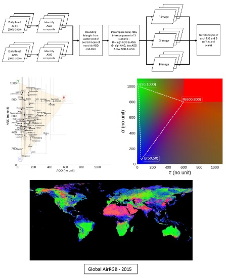
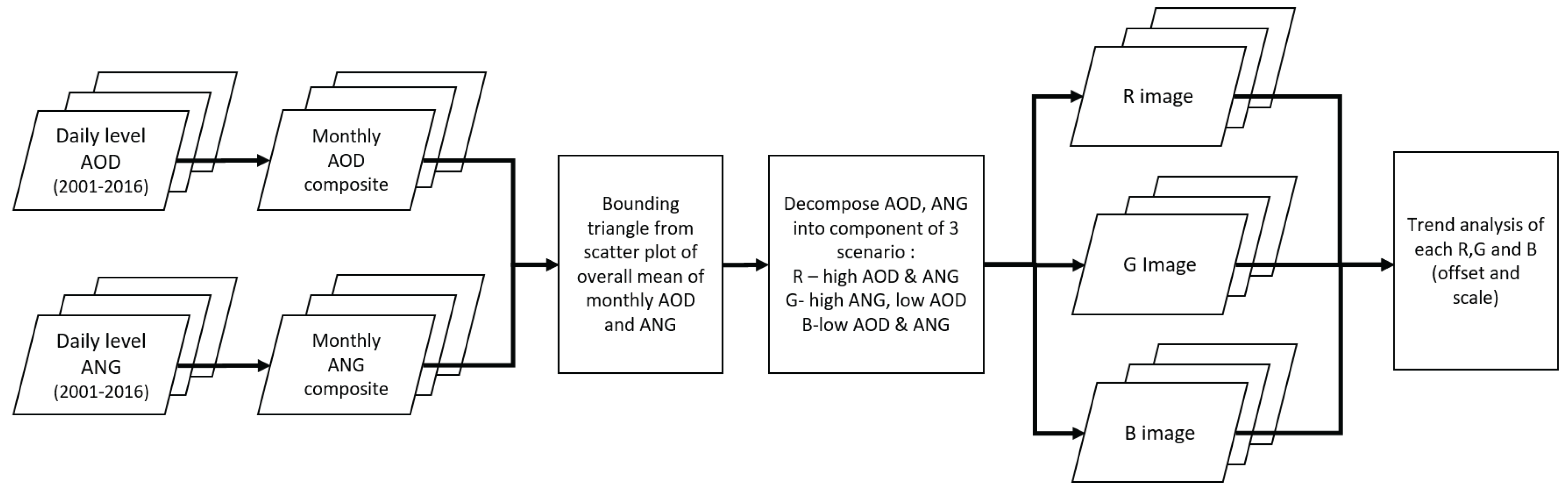
Figure 2 lays down the flowchart of data processing and analysis to obtain results.
2.2. Datasets Used
Retrieval of AOD and was based on Level2 Atmosphere Daily Global Product ‘MOD04L2’ Collection6 obtained from the Moderate Resolution Imaging Spectroradiometer (MODIS) sensor onboard NASA’s Earth Observing System (EOS) Terra satellite. Terra has a sun synchronous, near polar circular orbit that passes over at approximately 10:30 a.m. local time. ‘Deep_Blue_Aerosol_Optical_Depth_550_Land’ dataset was used for AOD images and ‘Deep_Blue_Angstrom_Exponent_Land’ dataset was used for images. MODIS was considered for its ability to provide spatially and temporally contiguous global coverage. To develop global daily products, cloud-free pixels (quality flag QA = 3) were considered and composited spatially. This daily data has a 10 km resolution and observes between 82 North to 82 South latitudes. The acquisition period consists of 16 years of datasets from January 2001 to December 2016. In this paper, we are converting MODIS observations to integer numbers by multiplying the float values by 1000.
Over bright surfaces (like urban areas) aerosol retrievals obtained from Deep Blue (DB) algorithm of MODIS show good agreement with those obtained by AERONET ground stations and are useful for urban areas [23]. DB performed better than the other dominant aerosol retrieval algorithm, Dark Target (DT), in Indo-Gangetic Plains [24]. The uncertainty of DB retrieval is dependent on geographical location and meteorological season. For example, Ginoux et al. [25] found that, while DB based AOD values were within the standard deviation of AERONET data in Africa, the Arabian Peninsula, and India, they were overestimated in California, Australia, and Israel. Payra et al. [26] observed dependence of estimation accuracies on Monsoon in a semi-arid urban region in India. In 2013, the second generation of DB (as part of Collection 6) was proposed [27], which used a hybrid approach to account for inhomogeneously vegetated urban/built-up areas among other improvements. In various regions of China, Tao et al. [28] found that although DB tends to underestimate AOD compared to DT, it provides a much larger sampling frequency in high aerosol loading conditions (AOD > 1) like regional haze pollution. Bilal and Nichol [29] found that DB retrieved AOD performed well compared to AERONET in the national capital region of China on both hazy and clear days, yet tended to overestimate during very polluted days (AOD > 1.5). The level of uncertainty of DB Collection 6 AOD retrievals (QA = 3) is approximately ±() [30], an improvement over Collection 5.1 uncertainty of ±() [31]. In Collection 6, a ‘best of’ AOD product also exists that combines AOD from DB and DT algorithms to estimate aerosol distribution over densely vegetated areas as well as bright surfaces. Sayer et al. [32] compared DB, DT as well as the combined DB-DT product and found that neither ‘consistently outperforms the other’. Although DB does give a higher fraction of observations agreeing with AERONET than DT, in very high AOD areas of South Asia DB tends to underestimate while DT tends to overestimate. The authors suggest that, in such areas, the combined product is likely to perform better than either DB or DT by canceling the opposing errors [32]. Therefore, further verification of the combined DB-DT product is desirable in terms of seasonality and long term trends, especially for Asian cities with evolving trends. Since, in this research, the area of interest is only urban/built-up regions, we have considered DB only, but there is also scope for the merged DB-DT product.
AOD and cannot be retrieved under cloudy sky conditions, as MODIS is an optical sensor. This results in significant reductions of cloud-free composites over equatorial regions of West Africa, South America, and Asia, as well as boreal regions of Europe and Canada [33]. To overcome this deficiency, usually a mean monthly composite is generated using daily images. Possible techniques include generating simple and quality weighted mean over a period of 16 days or 30 days [34], n-day composites on a rolling basis [33] and pixel coverage threshold monthly mean [35]. However, final values between these images can vary as much as 30% and, in light of different biases involved in each of these methods, Levy et al. [35], have noted that neither technique can be adjudged superior to another. In this research, a simple mean of daily images has been considered to obtain monthly datasets.
For validation of the proposed technique, measurement of PM2.5 from Beijing was used. Beijing was considered, since it is one of the few highly polluted cities with a publicly available and long-running PM2.5 measurements from a ground monitoring sensor. The sensor is installed at the United States’ embassy in the Chaoyang district (latitude −39.95, longitude −116.47), Beijing [36] and the observation dataset is available online [37]. The dataset consists of daily hourly measurements since May 2008. Although this data is not fully verified, previous studies have demonstrated its close correspondence with citywide PM2.5 concentrations [38,39]. For our study, we only considered ‘valid’ (quality flag) measurements made at 10:00 a.m. between May 2008 and December 2016.
2.3. AirRGB Decomposition and Visualization
Global aerosols have been visualized using color schemes in earlier research works to obtain more information. For example, Putman et al. [40] studied the effect of local emissions and large-scale weather systems on column CO mixing ratios by portraying global clouds (white) and aerosols (sulfate (blue), dust (brown) and carbon (green) from GEOS-5 model simulation. Penning de Vries et al. [41] determined the aerosol type by making use of trace gas abundance, aerosol absorption, mean aerosol size and MODIS derived AOD and to represent desert dust (red), biomass burning smoke (gray), secondary biogenic aerosols (green) and sea salt (blue).
Mukai et al. [42] and Sano et al. [43] used about three years of daily AOD and observation in urban Osaka, Japan to cluster aerosols into dust episodes, anthropogenic aerosol events and background clear atmosphere. The scatter points tended to lie within a triangular space when plotted over an and AOD orthogonal axes. Vertices of the said triangle represent three diverse scenarios corresponding to very high and low AOD value regime (signifying high composition of fine mode particles by anthropogenic contribution in emissions), high AOD value regime (signifying high aerosol levels in general), and low and low AOD value regime (signifying clean air quality).
In this paper, a three component decomposition technique called ‘AirRGB’ for visualizing aerosols to study trend of aerosols in urban regions has been proposed. The key idea was representing proximity of AOD and values to the three scenarios by decomposing it into three components. The three components are visualized by representing corresponding channels over a three-channel red-green-blue (RGB) scale varying from 0 to 100. In the AirRGB technique, we consider AOD and value as a Cartesian coordinate—(AOD, ) and refer to it as an ‘aerosol coordinate’. A bounding triangle is chosen such that, for each location, monthly aerosol coordinates shall lie within the triangle as much as possible. After setting the bounding triangle, aerosol coordinate is then transformed into a three-element vector that contains distance metrics from each vertex of the triangle. Since urban locations seldom show very high AOD and low unless regularly affected by dust storms, this scenario is not represented. Aerosol coordinates of each location is transformed onto a RGB scale to represent its ‘closeness’ to each scenario. The transformation procedure is discussed in detail in the following steps:
- For each urban location, the overall mean of monthly (from year 2001 to 2016) and AOD values of its central pixel were plotted on y and x-axis, respectively. The central pixel refers to the pixel corresponding to the city center. It was chosen to deal with cities (specially megacities) that are spread across several MODIS pixels (e.g., New York). This scheme is unlikely to affect the AOD and estimates since neighboring pixels have similar values over an urban area [44].
- Consider a bounding triangle, , such that its vertices corresponding to a) high and high AOD, (b) high and low AOD and, (c) low and low AOD are labeled as , , and , respectively. and B correspond to the colors red, green and blue (the color assigned to the vertex is irrelevant, but, in this paper, it is considered in the same fashion to ensure consistency).
- For any coordinate C () lying inside , decompose it over 3-band RGB-scale by first computing its distance metric from each vertex ( and B) as and . Thereafter, a distance vector l is derived by normalizing each distance metric by the side opposite to the corresponding vertex in , i.e., and , respectively. l is given for a general point coordinate C as:whereFor intuitive understanding of Equation (3), suppose that proximity of C is increasing to a vertex of . Then, components of l corresponding to other vertices will start decreasing to zero. The distance components for any vertex is in fact the sum of the area of two rectangles formed between C and each of the other vertices. For example, in Figure 3, component is the sum of yellow and green rectangles. Note that as C approaches towards either R or B vertices, linearly reduces to zero.
- For RGB color representation, values for channel [R, G, B] are normalized by maximum possible distance vector and multiplied by 100. It is given as:where
- For locations whose aerosol coordinates lie outside , is set as per the following rule:
AirRGB decomposition can be interpreted as a transformation technique using any aerosol coordinate (i.e., AOD and combination) that can be mapped onto a RGB scale. On this scale, high values () of a component imply significant closeness towards the corresponding scenario. Note that, if any component has a value , other components will be <50. Additionally, if values of all three components are <50, then a careful interpretation is needed since aerosol coordinates lie in the central region of the triangle and do not show proximity to any scenarios. For example, if B is trending to high values (), it indicates that the aerosol concentration is decreasing and the dominant aerosol mode is gradually shifting towards mineral aerosol (e.g., dust, etc.). This holds irrespective of R or G value. On the other hand, decreasing value or a low value of B only indicates that it is approaching a poor air quality regime. Only considering this information does not tell us whether this is due to anthropogenic emissions or mineral dusts unless R or G values are also probed simultaneously. It should be noted that, since it is a triangular space, the values of RGB components are not independent. Therefore, in Figure 3, it is impossible for C to trend in such a way that only one of the components change.
2.4. Uncertainty Estimation and Validation
The uncertainty in the AOD () from DB is ±() [30] as discussed before. We used the uncertainty calculated from DT, which is 0.4 [45], since we could not find literature supporting uncertainty of () derived from DB. Equation (6) was derived to estimate uncertainty () in R, G and B based on error propagation in Equation (3):
The R, G and B values obtained in the previous Section are validated with PM2.5 values using Beijing as a test case. Daily observations of R, G and B were plotted against corresponding PM2.5 measurements. Since PM2.5 sensor provides roadside measurements rather than background measurements, we expected consideration variation in the distribution of the plot. To overcome these mean values at range intervals of 25, g/m of PM2.5 were also plotted.
3. Result and Discussion
3.1. AirRGB Decomposition Parameters
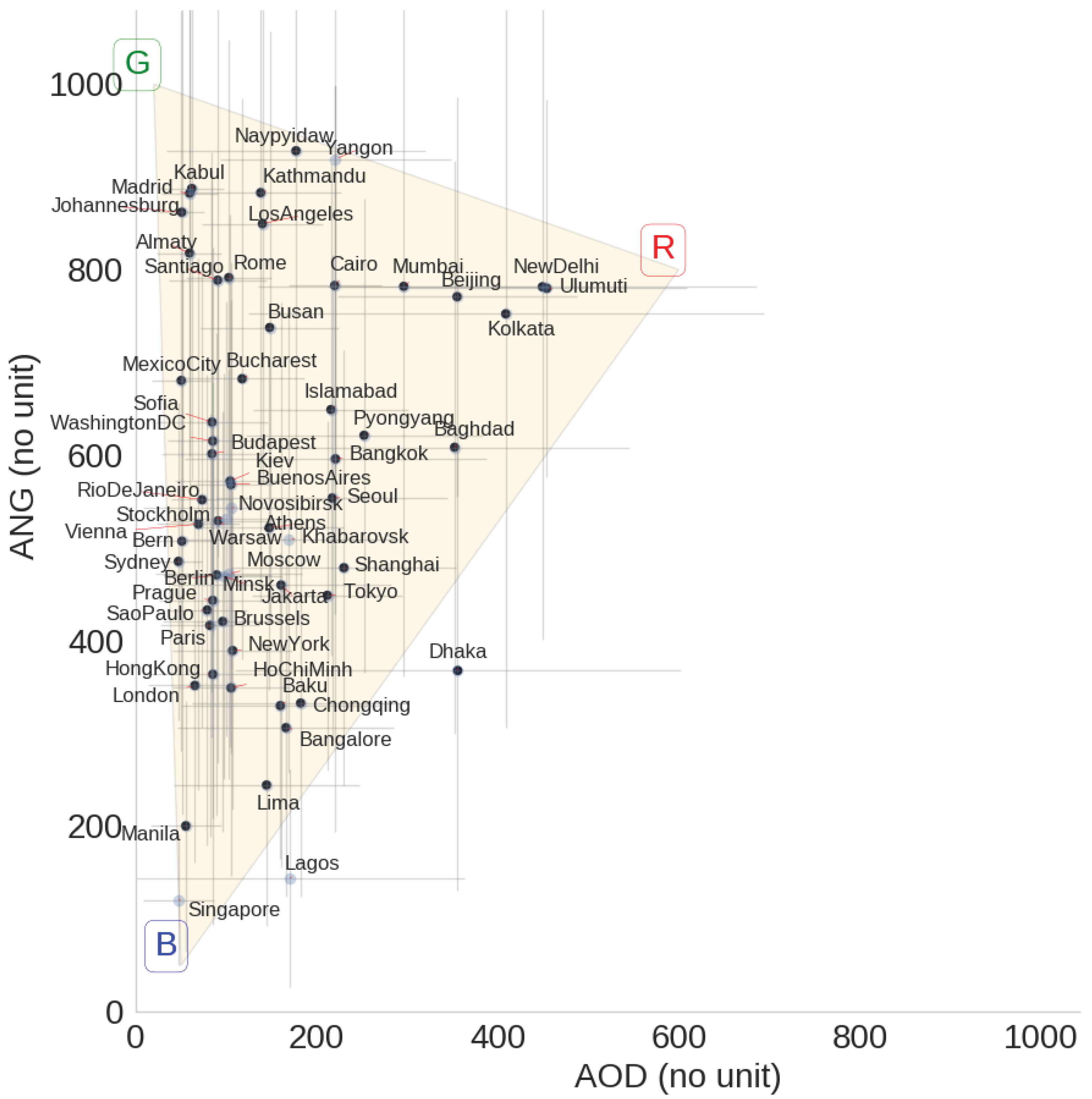
Figure 4 shows a scatter plot of mean AOD and mean and respective standard deviations (over the mean monthly values from January 2001 to December 2016) for all locations. The aerosol coordinates are scattered within an approximate triangular space, vertices of which correspond to the three scenarios discussed earlier in Section 2.3. It can also be seen that many cities from developed countries, e.g., Busan, Sydney, Los Angeles, Madrid, etc., have low AOD yet high values, while cities of rapidly developing countries (India and China) generally constitute the rightmost vertex of the triangle (R) that signifies high AOD and high . Most cities have large standard deviation along than AOD. This is expected to result in variations in time-series of G and B values. However, if a large standard deviation in AOD is also present, it will result in fluctuations of R and G values. Generally, a high standard deviation would imply a large change in aerosol levels either compared to its historic levels or strong annual seasonal variations. In Figure 4, if a standard deviation bar of a city exceeds the AirRGB triangle, then extreme values of either of R, G or B shall be obtained.
Based on the distribution of scatter points as discussed in Section 2.3 and as observed in Figure 4, aerosol coordinates of vertices of AirRGB bounding triangle were identified as and for red, green and blue channels, respectively. Two cities lay outside the triangular space: Lagos and Dhaka. Lagos’ valid observations were less than 48 months (four years) out of the total 16 years of observations and were not considered as reliable.
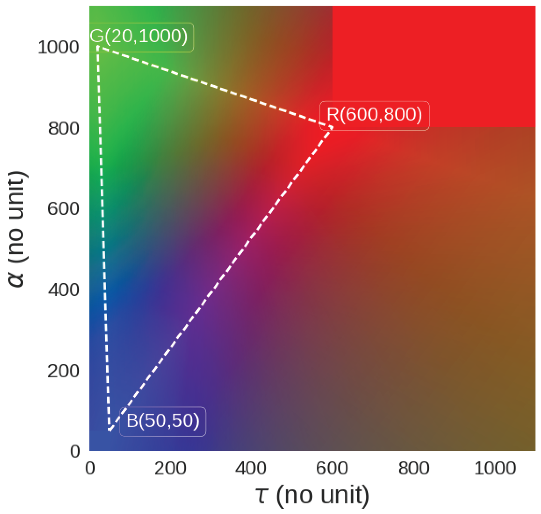
The transformation scale based on the vertex parameters of the AirRGB triangle is visualized in Figure 5. The values of the vertices R, G and B (based on Equation (4)) are respectively: , and . Points lying far outside the triangle are not covered by the three scenarios, except for those discussed in Equation (5).
3.2. Global AirRGB Visualization
The global AirRGB visualization map is shown at five-year intervals beginning in 2001 in Figure 6. It is easy to locate the highly polluted regions across East China and the Indian subcontinent, which show up in a bright red color (high R value). Furthermore, between the year 2010 and 2015, falling anthropogenic pollution in the Chinese urban region can be seen by a decreased intensity of red over Eastern China. In the same period, man-made pollution increased to an intense red in North India, West Asia and Central-West Africa and Central South America. Most regions across Western Europe, North America and South Japan are combinations of blue and green, inclined towards the former. This shows that, although industrial emissions are active, their levels are relatively lower than the regions discussed before.
While this paper does not focus on non-urban areas like dense vegetation and deserts, we would like to point out that application of the AirRGB technique over such regions may sometimes cause difficulty in interpreting values. This is likely to happen since AOD and characteristics of such areas lie far beyond the bounding AirRGB triangle. For instance, the dusty Australian desert has an AOD in the range of 100 to 250 [25], but its lies far above 1000, resulting in bright green (high value of G). This is clearly misleading. Values of AOD and over other prominent desert regions like the Sahara desert, the Arabian desert, the Thar desert and parts of the Gobi desert also lie outside the AirRGB triangle but still show up in red due to proximity to the vertex R. Furthermore, DB retrieves only under bright surfaces in the visible wavelength. Thus, data over regions with extensive biomass or dense vegetation like Central Africa and Amazon cannot be retrieved completely since their surface reflectances in the visible are less than 0.15 [25]. Here, the DB sampling rate is much less and often of poor quality as compared to DT. This also leads to underestimation in the mean monthly images prepared by us. Furthermore, a bright green strip can be seen in the Western Asia in the Red Sea as well as the Persian Gulf. Although there are no urban centers of interest here, we suspect it has high G value on account of fine mode aerosols of sulphur dioxide emissions from oil refineries in this area [46,47]. Thus, to incorporate effective representation of non-urban regions, the AirRGB triangle with different vertex parameters can be specified using aerosol coordinates from such pixels.
3.3. AirRGB Trend of Cities
We further discuss variation in urban air quality due to anthropogenic causes using AirRGB decomposition. We first investigated representative cities lying near the vertices of AirRGB bounding triangle in Figure 4: New Delhi (highest R value), Madrid (highest G value) and Manila (highest B value). A four-month moving average of their R, G, B values was plotted and shown in Figure 6.
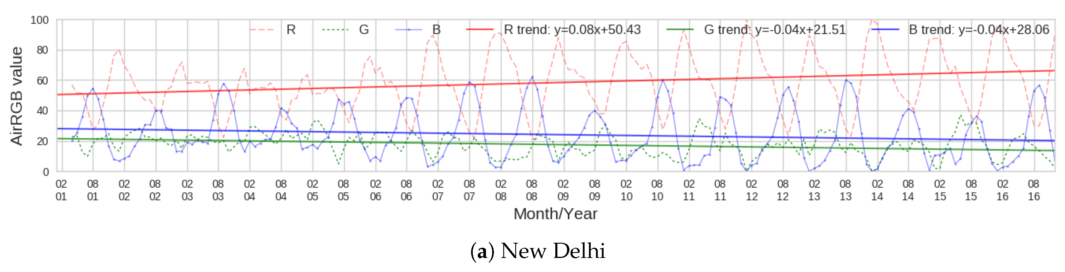
Air quality in New Delhi, which is located in the Indo-Gangetic Plains, undergoes strong seasonal variations. From Figure 7a, rapidly rising R values (slope is 0.08) can be noticed distinctly. High R (≥50) values are a seasonal phenomena that have been rising even further since 2009. This establishes that contribution and concentration of fine mode particles is rising gradually in these places. The annual maximum value of R occurs around the December–January period, while the lowest values are seen in August–September. B values have been decreasing (slope is −0.04), with high B values (∼50) rarely being seen except peak Monsoon season month (July). This signifies a constant presence of aerosols due to anthropogenic emissions, which undergo wet scavenging in rain. High peaks of G are observed frequently in the September months, which is caused by biomass burning after the harvesting season in neighboring farmlands.
In contrast to New Delhi, RGB components of Madrid (Figure 7b) did not show any seasonality. Low R values (<10) signify low aerosol loading, but G values are much higher (∼70) than other components, signifying a large contribution of anthropogenic emissions (mostly vehicular) to urban aerosol levels. This has also been confirmed by Borge et al. [48] as a violation of NO standards. At certain events, air quality also tends to become very clean, as evidenced by transition from high G value to high B value in January–February of 2003, 2004, 2010, 2013, 2014 and 2016.
Manila (Figure 7c) has very clean air with low aerosol emissions in the early part of the observation period. This was seen from high offset of B (∼76) and very low offset of R (∼4) and G (∼12) values. However, there is also a sharp fall in B level (slope = −0.06).
As cases, we focus on the Asian cities of Beijing, Tokyo and Dhaka. In Figure 7d, it was observed that traditionally high R values are decreasing in Beijing. This has especially become apparent after the year 2011 when higher values of B can also be seen. It was noteworthy that, during the month of August in 2008, R value suddenly drops to much lower than what is expected during this time of year. This was likely due to the 2008 Beijing Olympics Games, during which several traffic and emission restrictions were strictly enforced from the period of April 2007 to January 2009, as has also been confirmed by Wang et al. [49].
Dhaka also presented an interesting case of varying air pollution. The initial decrease in R between 2001 and 2005 has been attributed to government policy intervention factors e.g., a ban on two stroke vehicles, and a promotion of compressed natural gas (CNG) as fuel and the control of industrial emission [50]. A rise in R can be seen post 2006, which has been attributed to a rise in emissions from brick factories, while the fall in R after 2011 is a result of efforts to convert petrol/diesel vehicles to CNG emissions [7]. It appears then that a rise in G despite a fall in R could largely be a cause of brick factories.
Among the four cities, Tokyo has the lowest R offset (∼30). Its B offset (47.83) is similar to that of Dhaka (50.28), but recent B values are much higher than the latter. Furthermore, air quality in Tokyo has been consistently improving, especially in the last 10 years, as represented by a positive slope of B (0.03) and negative slopes of R (−0.01) and G (−0.02).
3.4. Global AirRGB Component Trend
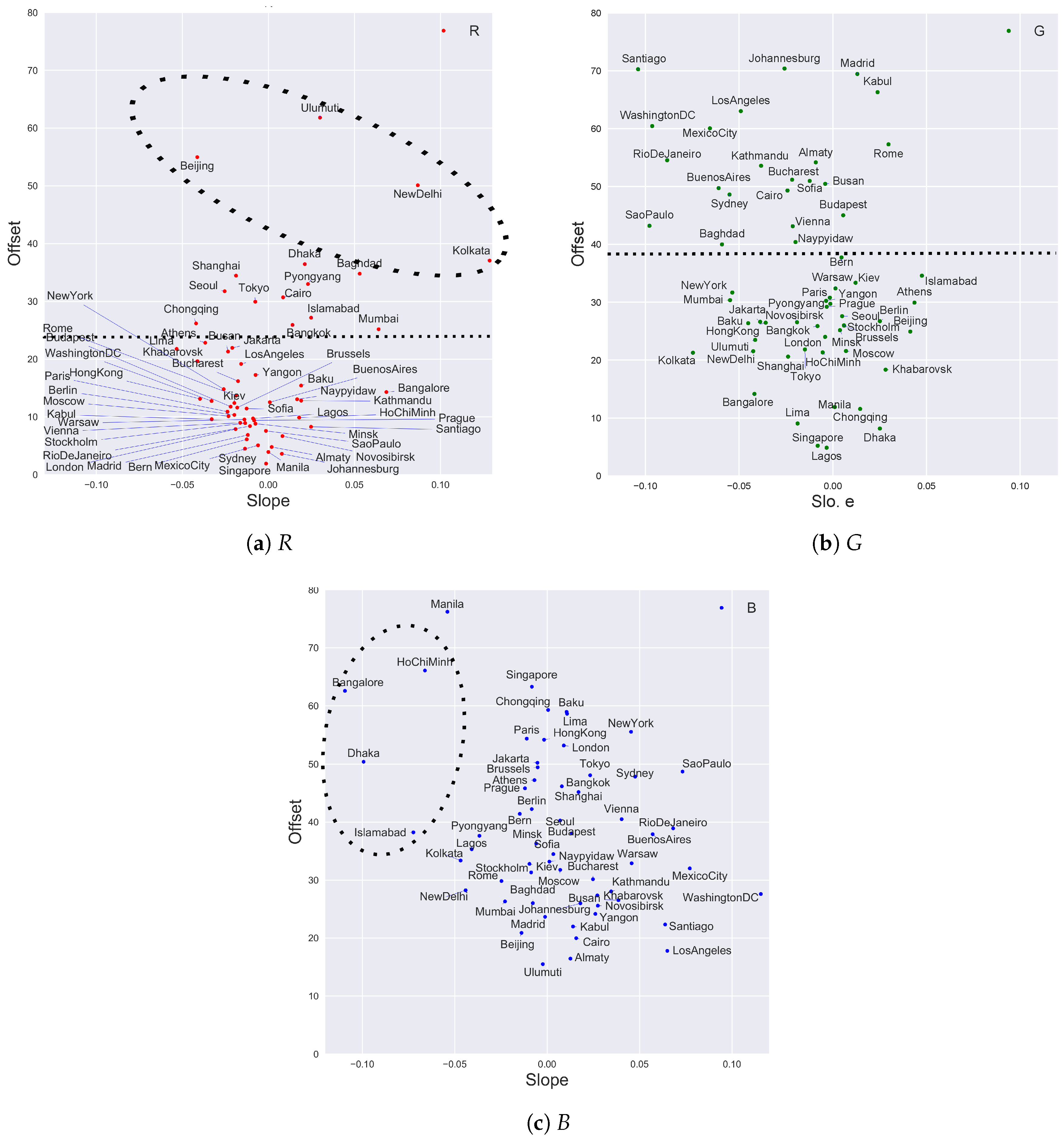
Global trends of AirRGB components of all locations under study were computed for each component using the least squares method over monthly composites from the year 2001 to 2016. Offset and slope of the best fit line for each city so obtained is shown in Figure 8. The offset corresponds to baseline levels of each RGB component while its slope depicts trends of the components.
3.4.1. Global Trend of R
In Figure 8a, a positive slope of R was observed for most Asian cities. Furthermore, all such cities belong to the developing countries located in South Asia and South East Asia (e.g., India, Nepal, Vietnam). Cities of North America (e.g., New York, Washington DC) and Europe (e.g., Brussels, Paris) were concentrated in a narrow region with a negative slope (between −0.03 and 0.00) and small offset (less than 16) except Athens and Los Angeles. Both Athens and Los Angeles count amongst the most polluted cities in Europe and North America on account of traffic and industrial emissions (Chaloulakou et al. [51], American Lung Association [52]). However, their offset was much less than that of Asian cities, which is mostly greater than 25. Notable outliers with large offsets include Beijing, Urumqi, New Delhi and Kolkata. Of these, only Beijing has a negative slope, as discussed previously. Several other cities in China (Shanghai, Chongqing) also have high offsets but negative slopes. This is likely an indication that although baseline aerosol levels in Chinese cities have historically been high, its air quality is improving. It is of further interest to identify factors leading to increase or decrease of slope in these cities.
3.4.2. Global Trend of G
Slope and offset G values of the cities (Figure 8b) show where fine mode aerosol dominates under low aerosol loading conditions. Unlike the plot for R, here European and North American cities were not concentrated in a well-defined region. This implies varying contributions of traffic and industrial emissions to urban pollution in cities in developed countries. However, based on offset values, two clusters of cities are visible (a) 70 to 40 and (b) 35 to 5. In the first cluster, it was hard to distinguish between cities from developed and developing countries. This implied that, even with cleaner air quality, fine mode aerosol from traffic and industrial emission can dominate. South American cities Rio de Janeiro, Buenos Aires and Sao Paulo were present in the former cluster and showed negative slopes. This is in agreement with issues associated with SO ( additionally CO for Sao Paulo) and PM2.5 levels caused by vehicular and industrial emissions as identified previously (Toledo et al. [53], Mage et al. [5], Bogo et al. [54]). The second cluster shows that cities like Tokyo and London have similar offsets (∼25) as Kolkata and Beijing. However, these cities have midrange offsets that lie along and close to the side in (Figure 5), and so analyzing the second cluster based on G values alone can lead to misleading conclusions.
3.4.3. Global Trend of B
In the offset and slope plot of global cities for B (Figure 8c), notable outliers existed in terms of slope. These were Ho Chi Minh, Bangalore, Dhaka and Islamabad. They have relatively high offset of B values (≥40) from historically anthropogenic polluting activities, but a large negative slope (≤0.07) indicates pollutants surging rapidly. In conjunction with their R and G plots, we find that they are rapidly moving towards high pollution and urban emissions in the following descending order: Bangalore, Islamabad, Ho Chi Minh and Dhaka. On the other hand, New York, Tokyo, Sydney and Sao Paolo have high B offsets (>45) but a positive B slope, which indicates that these cities not only had low aerosol levels but are still achieving cleaner air. All South American cities are also on a rapid course to achieving high B values.
In some cities like Kabul and Baghdad, not much literature is available regarding air quality trend of anthropogenic emissions. For instance, we inferred domination of primary fine mode aerosol at Kabul based on its high offset (∼65) and positive slope (∼0.03) of G value. This inference is similar to [55], who collected samples at urban locations in Kabul but unlike that realized by [56], who used two weeks of data monitored at military camps). For Baghdad, high R and G values point to a presence of mineral dust and fine aerosols. This is in conjunction with [57], who identified the dominant sources to be dust and carbonaceous aerosols (gasoline and diesel engines) using source apportionment study.
The AirRGB technique provides a strong hint of emission issues by visualizing which of the three representative scenarios are prime in the city. Trends of R, G and B help identify the effect of a policy intervention, conclusions based on which can lead to establishing more robust ground monitoring sensor systems and systematic control of air quality by city authorities.
3.5. Uncertainty and Validation
3.5.1. Uncertainty
Using Equation (6) and AirRGB parameters, the maximum uncertainties in R, G and B were computed as: and . We would like to point that these uncertainties are dependent on values of AOD, and we used the values of the vertex to compute corresponding uncertainties. Although R’s uncertainty is the lowest amongst the three, it can considerably impact interpretation drawn from Figure 8a, especially those locations showing a high standard deviation in their AOD. The high uncertainty in G and B values is on account of the uncertainty in .
3.5.2. Validation
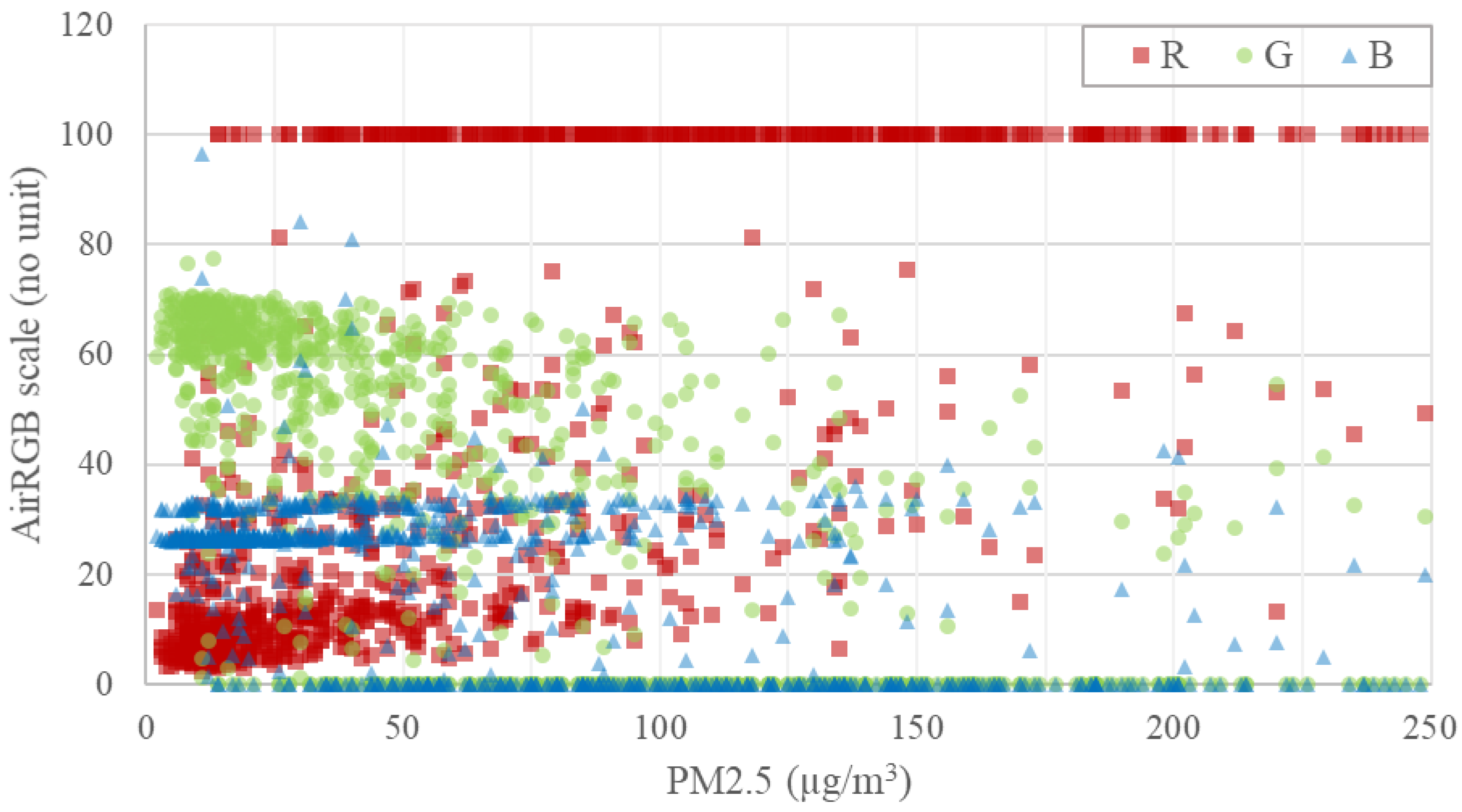
Nine hundred forty-five data points from Beijing with valid concurrent PM2.5 and AirRGB observations were found. They are plotted in Figure 9. A clear separation between AirRGB components can be seen with respect to PM2.5 values. Many B values occurred between the two bands 20 and 40 for a wide range of PM2.5. This occurs because Deep Blue algorithm caps extremely high at 1.8 and fixes it to 1.5 during very low AOD conditions [31]. Several R values equal to 100 are easily noticeable because Beijing is located almost near the R vertex in the AirRGB triangle. Thus, aerosol coordinates lying beyond the vertex result in higher prominence of R equal to 100. Contrary to expectations, high R values were found during some low PM2.5 (<50 g/m) measurements while B reached moderate levels during high PM2.5 (>100 g/m) measurements. This is probably due to the difference between a ground monitoring sensor (which is affected local events) and a coarse resolution satellite sensor (reflecting observation over a 10 km region).
To further analyze AirRGB, we tried overcoming the difference in spatial sampling by considering mean values, as shown in Table 1. Data points get sparse with higher PM2.5 values. When PM2.5 is between 0 and 50 g/m, G has the highest value, implying the absence of coarse particles and aerosol loading, mostly on account of fine mode particles. Despite low values of PM2.5, B rarely gets beyond 25. Thus, even when PM2.5 is low, Beijing’s air quality may still not be as breathable as in other cities with higher B values (e.g., London, New York). As PM2.5 rises beyond 50 g/m, high mean R values are seen, which approach 100 as PM2.5 goes further beyond 150 g/m.
In Beijing’s case, R values showed close agreement with PM2.5 ( ) and a high coefficient of agreement (0.97). This relation might be unique for Beijing since other cities may have different emission characteristics and consequently different relationships between PM2.5 and R, G and B. One of the ways to assess this could be to simulate PM2.5 and PM10 generated using chemistry transport models (e.g., WRF-Chem, CMAQ) at different spatial resolutions [58]. A multi-sensor fusion approach can be also be taken to incorporate other crucial information such as planetary boundary layer height, relative humidity, season, and other geographical attributes of monitoring sites. CALIPSO (Cloud-Aerosol Lidar and Infrared Pathfinder Satellite Observations), an active remote sensing satellite, can be useful in this regard. To resolve coverage issues, aerosol data products from VIIRS (Visible Infrared Imaging Radiometer Suite) are gaining popularity.
One of the most prospective applications of this research can be to generate high resolution AirRGB maps to depict variation in air quality across regions with different characteristics in a city. This can bring out the variation in aerosols over residential, commercial and industrial areas, as they are likely to have different emission sources.
4. Conclusions
In this paper, a novel visualization and monitoring scheme called AirRGB has been proposed that decomposes AOD and Angstrom exponent into three components (labelled as R, G and B) corresponding to three scenarios: high pollution regime (R), clean air dominated by fine mode aerosols (G) and clean air (B). AirRGB contains more interpretable information than a conventional visualization. We used 16 years of AOD and Angstrom exponent () retrievals from MODIS sensor and analyzed trend of their R, G and B components. We identified that, in contrast to European and North American cities, high overall background pollution exists in Asian cities (except Tokyo). Analysis of Asian cities reveals decreasing overall aerosol loading in Tokyo and the opposite scenario for New Delhi and Dhaka. Beijing has started showing an improvement in aerosol concentrations in terms of R values, but rising G values indicate that anthropogenic pollution is still the dominant mode.
In this research, daily levels of AOD and retrievals were composited at the mean monthly scale by considering only cloud free pixel values. This is likely to bias the composite image to some extent, since aerosol concentrations during cloudy days are not considered. Furthermore, uncertainties in AOD and retrievals themselves also lead to uncertainties in R, G and B, which were computed to be and , respectively. Therefore, AirRGB parameters and inferences must be further investigated by considering datasets derived from other techniques of compositing means, such that this bias can be removed.
AirRGB trends inform us about the nature of urban air quality but not about the underlying cause. As a future step, AirRGB components can be linked with energy consumption and economic growth to understand how long-term air quality evolves in urban environments. Nightlight observed from space, e.g., VIIRS DNB satellite images, can be used in this regard, since it is correlated with socio-economic indicators like vehicle count, energy use, GDP, etc. [59]. Analyzing long-term air quality trends with nightlight brightness can inform about how the cause of pollution is changing with socio-economic development [60]. Similarly, AirRGB can also be analyzed with nightlight images observed from space. It can help in studying which of the three scenarios represented by AirRGB decomposition is affected by socio-economic development.
Acknowledgments
This research was in part supported by the Monbukagakusho (MEXT) scholarship.
Author Contributions
A.F. and W.T. conceived and designed the experiments; P.M. and A.F. performed the experiments; P.M. and W.T. analyzed the data; W.T. prepared the base datasets; P.M. wrote the paper and all authors read the paper and provided revision suggestions.
Conflicts of Interest
The authors declare no conflict of interest.
References
- United Nations General Assembly. Transforming Our World: The 2030 Agenda for Sustainable Development. 2015. Available online: http://www.un.org/ga/search/viewdoc.asp?symbol=A/RES/70/1 (accessed on 2 August 2017).
- World Health Organization. Ambient (Outdoor) Air Pollution in Cities Database 2014. Available online: http://www.who.int/phe/healthtopics/outdoorair/databases/cities-2014/en/ (accessed on 2 August 2017).
- Takemura, T.; Uno, I.; Nakajima, T.; Higurashi, A.; Sano, I. Modeling study of long-range transport of Asian dust and anthropogenic aerosols from East Asia. Geophys. Res. Lett. 2002, 29, 11-1–11-4. [Google Scholar]
- Mayer, H. Air pollution in cities. Atmos. Environ. 1999, 33, 4029–4037. [Google Scholar]
- Mage, D.; Ozolins, G.; Peterson, P.; Webster, A.; Orthofer, R.; Vandeweerd, V.; Gwynne, M. Urban Air Pollution in Megacities of the World. Atmos. Environ. 1996, 30, 681–686. [Google Scholar]
- Srivastava, A.; Gupta, S.; Jain, V.K. Source Apportionment of Total Suspended Particulate Matter in Coarse and Fine Size Ranges Over Delhi. Aerosol Air Qual. Res. 2008, 8, 188–200. [Google Scholar]
- Begum, B.A.; Biswas, S.K.; Hopke, P.K. Key issues in controlling air pollutants in Dhaka, Bangladesh. Atmos. Environ. 2011, 45, 7705–7713. [Google Scholar]
- Castanho, D.A.A.; Artaxo, P. Wintertime and summertime Sao Paulo aerosol source apportionment study. Atmos. Environ. 2001, 35, 4889–4902. [Google Scholar]
- Zhang, R.; Jing, J.; Tao, J.; Hsu, S.; Wang, G.; Cao, J.; Lee, C.; Zhu, L.; Chen, Z.; Zhao, Y.; et al. Chemical characterization and source apportionment of PM2.5 in Beijing: Seasonal perspective. Atmos. Chem. Phys. 2013, 13, 7053–7074. [Google Scholar]
- Belis, C.A.; Karagulian, F.; Larsen, B.R.; Hopke, P.K. Critical review and meta-analysis of ambient particulate matter source apportionment using receptor models in Europe. Atmos. Environ. 2013, 69, 94–108. [Google Scholar]
- Baldasano, J.M.; Valera, E.; Jiménez, P. Air quality data from large cities. Sci. Total Environ. 2003, 307, 141–165. [Google Scholar]
- Gupta, P.; Christopher, S.A.; Wang, J.; Gehrig, R.; Lee, Y.; Kumar, N. Satellite remote sensing of particulate matter and air quality assessment over global cities. Atmos. Environ. 2006, 40, 5880–5892. [Google Scholar]
- Gurjar, B.R.; Butler, T.M.; Lawrence, M.G.; Lelieveld, J. Evaluation of emissions and air quality in megacities. Atmos. Environ. 2008, 42, 1593–1606. [Google Scholar]
- Ångström, A. On the atmospheric transmission of Sun radiation and on dust in the air. Geogr. Ann. 1929, 11, 156–166. [Google Scholar]
- Dubovik, O.; Holben, B.; Eck, T.F.; Smirnov, A.; Kaufman, Y.J.; King, M.D.; Tanré, D.; Slutsker, I. Variability of Absorption and Optical Properties of Key Aerosol Types Observed in Worldwide Locations. J. Atmos. Sci. 2002, 59, 590–608. [Google Scholar]
- Eck, T.F.; Holben, B.N.; Reid, J.S.; Dubovik, O.; Smirnov, A.; O’Neill, N.T.; Slutsker, I.; Kinne, S. Wavelength dependence of the optical depth of biomass burning, urban, and desert dust aerosols. J. Geophys. Res. 1999, 104, 31333. [Google Scholar]
- Nakajima, T.; Higurashi, A. A use of two-channel radiances for an aerosol characterization from space. Geophys. Res. Lett. 1998, 25, 3815–3818. [Google Scholar]
- Eldering, A.; Cass, G.R. An air monitoring network using continuous particle size distribution monitors: Connecting properties to visibility via Mie scattering calculations. Atmos. Environ. 1994, 28, 2733–2749. [Google Scholar]
- Baumer, D.; Vogel, B.; Versick, S.; Rinke, R.; Mohler, O.; Schnaiter, M. Relationship of visibility, aerosol optical thickness and aerosol size distribution in an ageing air mass over South-West Germany. Atmos. Environ. 2008, 42, 989–998. [Google Scholar]
- NASA Worldview. Available online: https://worldview.earthdata.nasa.gov/ (accessed on 2 August 2017).
- NASA Earthdata Giovanni. Available online: https://giovanni.gsfc.nasa.gov/giovanni/ (accessed on 2 August 2017).
- United Nations. World Economic Situation Prospects 2014; United Nations Publication: New York, NY, USA, 2014. [Google Scholar]
- Hsu, N.C.; Tsay, S.C.; King, M.D.; Member, S.; Herman, J.R. Aerosol Properties Over Bright-Reflecting Source Regions. IEEE Trans. Geosci. Remote Sens. 2004, 42, 557–569. [Google Scholar]
- Bibi, H.; Alam, K.; Chishtie, F.; Bibi, S.; Shahid, I.; Blaschke, T. Intercomparison of MODIS, MISR, OMI, and CALIPSO aerosol optical depth retrievals for four locations on the Indo-Gangetic plains and validation against AERONET data. Atmos. Environ. 2015, 111, 113–126. [Google Scholar]
- Ginoux, P.; Prospero, J.M.; Gill, T.E.; Hsu, N.C.; Zhao, M. Global-scale attribution of anthropogenic and natural dust sources and their emission rates based on modis deep blue aerosol products. Rev. Geophys. 2012, 50, 1–36. [Google Scholar]
- Payra, S.; Soni, M.; Kumar, A.; Prakash, D.; Verma, S. Intercomparison of Aerosol Optical Thickness Derived from MODIS and in Situ Ground Datasets over Jaipur, a Semi-arid Zone in India. Environ. Sci. Technol. 2015, 49, 9237–9246. [Google Scholar]
- Hsu, N.C.; Jeong, M.J.; Bettenhausen, C.; Sayer, A.M.; Hansell, R.; Seftor, C.S.; Huang, J.; Tsay, S.C. Enhanced Deep Blue aerosol retrieval algorithm: The second generation. J. Geophys. Res. Atmos. 2013, 118, 9296–9315. [Google Scholar]
- Tao, M.; Chen, L.; Wang, Z.; Tao, J.; Che, H.; Wang, X.; Wang, Y. Comparison and evaluation of the MODIS Collection 6 aerosol data in China. J. Geophys. Res. Atmos. 2015, 120, 6992–7005. [Google Scholar]
- Bilal, M.; Nichol, J.E. Evaluation of MODIS aerosol retrieval algorithms over the Beijing-Tianjin-Hebei region during low to very high pollution events. J. Geophys. Res. Atmos. 2015, 120, 7941–7957. [Google Scholar]
- Sayer, A.M.; Hsu, N.C.; Bettenhausen, C.; Jeong, M.J.; Meister, G. Effect of MODIS Terra radiometric calibration improvements on Collection 6 Deep Blue aerosol products: Validation and Terra/Aqua consistency. J. Geophys. Res. Atmos. 2015, 120, 157–174. [Google Scholar]
- Sayer, A.M.; Hsu, N.C.; Bettenhausen, C.; Jeong, M. Validation and uncertainty estimates for MODIS Collection 6 “Deep Blue” aerosol data. J. Geophys. Res. Atmos. 2013, 118, 7864–7872. [Google Scholar]
- Sayer, A.M.; Munchak, L.A.; Hsu, N.C.; Levy, R.C.; Bettenhausen, C.; Jeong, M. MODIS Collection 6 aerosol products: Comparison between Aqua’s e-Deep Blue, Dark Target, and “merged” data sets, and usage recommendations. J. Geophys. Res. Atmos. 2014, 119, 13965–13989. [Google Scholar]
- Roy, D.P.; Lewis, P.; Schaaf, C.B.; Devadiga, S.; Boschetti, L. The global impact of clouds on the production of MODIS bidirectional reflectance model-based composites for terrestrial monitoring. IEEE Geosci. Remote Sens. Lett. 2006, 3, 452–456. [Google Scholar]
- Hubanks, P.; Platnick, S.; King, M.; Ridgway, B. MODIS Atmosphere L3 Gridded Product Plgorithm Pheoretical Basis Document (ATBD) & Users Guide. 2016. Available online: https://modis-images.gsfc.nasa.gov/_docs/L3_ATBD_C6.pdf (accessed on 2 August 2017).
- Levy, R.C.; Leptoukh, G.G.; Kahn, R.; Zubko, V.; Gopalan, A.; Remer, L.A. A critical look at deriving monthly aerosol optical depth from satellite data. IEEE Trans. Geosci. Remote Sens. 2009, 47, 2942–2956. [Google Scholar]
- U.S. Department of State. U.S Embassy Beijing Air Quality Monitor. Available online: https://china.usembassy-china.org.cn/embassy-consulates/beijing/air-quality-monitor (accessed on 2 August 2017).
- U.S. Department of State. Beijing—PM2.5. Available online: http://www.stateair.net/web/post/1/1 (accessed on 2 August 2017).
- Wang, J.F.; Hu, M.G.; Xu, C.D.; Christakos, G.; Zhao, Y. Estimation of Citywide Air Pollution in Beijing. PLoS ONE 2013, 8, 1–6. [Google Scholar]
- Jiang, J.; Zhou, W.; Cheng, Z.; Wang, S.; He, K.; Hao, J. Particulate Matter Distributions in China during a Winter Period with Frequent Pollution Episodes (January 2013). Aerosol Air Qual. Res. 2015, 10, 494–503. [Google Scholar]
- Putman, W.M.; Ott, L.; Darmenov, A.; da Silva, A. A global perspective of atmospheric carbon dioxide concentrations. Parallel Comput. 2016, 55, 2–8. [Google Scholar]
- Penning de Vries, M.J.M.; Beirle, S.; Hörmann, C.; Kaiser, J.W.; Stammes, P.; Tilstra, L.G.; Tuinder, O.N.E. A global aerosol classification algorithm incorporating multiple satellite data sets of aerosol and trace gas abundances. Atmos. Chem. Phys. 2015, 15, 10597–10618. [Google Scholar]
- Mukai, S.; Nishina, M.; Sano, I.; Mukai, M.; Iguchi, N.; Mizobuchi, S. Suspended particulate matter sampling at an urban AERONET site in Japan, part 1: Clustering analysis of aerosols. J. Appl. Remote Sens. 2007, 1, 13518. [Google Scholar]
- Sano, I.; Mukai, M.; Iguchi, N.; Mukai, S. Suspended particulate matter sampling at an urban AERONET site in Japan, part 2: Relationship between column aerosol optical thickness and PM2.5 concentration. J. Appl. Remote Sens. 2010, 4, 43504. [Google Scholar]
- Mi, W.; Li, Z.; Xia, X.; Holben, B.; Levy, R.; Zhao, F.; Chen, H.; Cribb, M. Evaluation of the Moderate Resolution Imaging Spectroradiometer aerosol products at two Aerosol Robotic Network stations in China. J. Geophys. Res. 2007, 112, 1–14. [Google Scholar]
- Levy, R.C.; Remer, L.A.; Kleidman, R.G.; Mattoo, S.; Ichoku, C.; Kahn, R.; Eck, T.F. Global evaluation of the Collection 5 MODIS dark-target aerosol products over land. Atmos. Chem. Phys. 2010, 10, 10399–10420. [Google Scholar] [Green Version]
- Klimont, Z.; Smith, S.J.; Cofala, J. The last decade of global anthropogenic sulfur dioxide: 2000–2011 emissions. Environ. Res. Lett. 2013, 8, 1–6. [Google Scholar]
- McLinden, C.A.; Fioletov, V.; Shephard, M.W.; Krotkov, N.; Li, C.; Martin, R.V.; Moran, M.D.; Joiner, J. Space-based detection of missing sulfur dioxide sources of global air pollution. Nat. Geosci. 2016, 9, 1–7. [Google Scholar]
- Borge, R.; Lumbreras, J.; Pérez, J.; de la Paz, D.; Vedrenne, M.; de Andrés, J.M.; Rodríguez, M.E. Emission inventories and modeling requirements for the development of air quality plans. Application to Madrid (Spain). Sci. Total Environ. 2014, 466–467, 809–819. [Google Scholar]
- Wang, S.; Zhao, M.; Xing, J.; Wu, Y.; Zhou, Y.; Lei, Y.; He, K.; Fu, L.; Hao, J. Quantifying the air pollutants emission reduction during the 2008 olympic games in Beijing. Environ. Sci. Technol. 2010, 44, 2490–2496. [Google Scholar]
- Begum, B.A.; Biswas, S.K.; Hopke, P.K. Assessment of trends and present ambient concentrations of PM2.2 and PM10 in Dhaka, Bangladesh. Air Qual. Atmos. Heal. 2008, 1, 125–133. [Google Scholar]
- Chaloulakou, A.; Kassomenos, P.; Spyrellis, N.; Demokritou, P.; Koutrakis, P. Measurements of PM10 and PM2.5 particle concentrations in Athens, Greece. Atmos. Environ. 2003, 37, 649–660. [Google Scholar]
- American Lung Association. State of the Air 2016; American Lung Association: Chicago, IL, USA, 2016. [Google Scholar]
- Toledo, V.E.; Almeida, P.B.; Quiterio, S.L.; Arbilla, G.; Moreira, A.; Escaleira, V.; Moreira, J.C. Evaluation of levels, sources and distribution of toxic elements in PM10 in a suburban industrial region, Rio de Janeiro, Brazil. Environ. Monit. Assess. 2008, 139, 49–59. [Google Scholar]
- Bogo, H.; Otero, M.; Castro, P.; Ozafrán, M.J.; Kreiner, A.; Calvo, E.J.; Negri, R.M. Study of atmospheric particulate matter in Buenos Aires city. Atmos. Environ. 2003, 37, 1135–1147. [Google Scholar]
- Wingfors, H.; Hägglund, L.; Magnusson, R. Characterization of the size-distribution of aerosols and particle-bound content of oxygenated PAHs, PAHs, and n-alkanes in urban environments in Afghanistan. Atmos. Environ. 2011, 45, 4360–4369. [Google Scholar]
- Magnusson, R.; Hägglund, L.; Wingfors, H. Broad exposure screening of air pollutants in the occupational environment of Swedish soldiers deployed in Afghanistan. Mil. Med. 2012, 177, 318–325. [Google Scholar]
- Hamad, H.S.; Schauer, J.J.; Heo, J.; Kadhim, A.K.H. Source apportionment of PM2.5 carbonaceous aerosol in Baghdad, Iraq. Atmos. Res. 2015, 156, 80–90. [Google Scholar]
- Baklanov, A.; Schlünzen, K.; Suppan, P.; Baldasano, J.; Brunner, D.; Aksoyoglu, S.; Carmichael, G.; Douros, J. Online coupled regional meteorology chemistry models in Europe: Current status and prospects. Atmos. Chem. Phys. 2014, 14, 317–398. [Google Scholar]
- Katayama, N.; Takeuchi, W. Comparison between Nighttime Light and Socioeconomic Indicators an International Scale Using VIIRS Day-Night Band. In Proceedings of the 35th Asian Conference on Remote Sensing, Nay Pyi Taw, Myanmar, 27–31 October 2014. [Google Scholar]
- Misra, P.; Takeuchi, W. Analysis of air quality and nighttime light for Indian urban regions. IOP Conf. Ser. Earth Environ. Sci. 2016, 37, 12077. [Google Scholar]
Figure 1.
Cities considered for analysis in this study. The city markers are sized as per vehicle population. The markers are shown in red if the national gross domestic product per capita (pc GDP, year 2015) is less than $12,000 otherwise, it is shown in green.
Figure 1.
Cities considered for analysis in this study. The city markers are sized as per vehicle population. The markers are shown in red if the national gross domestic product per capita (pc GDP, year 2015) is less than $12,000 otherwise, it is shown in green.
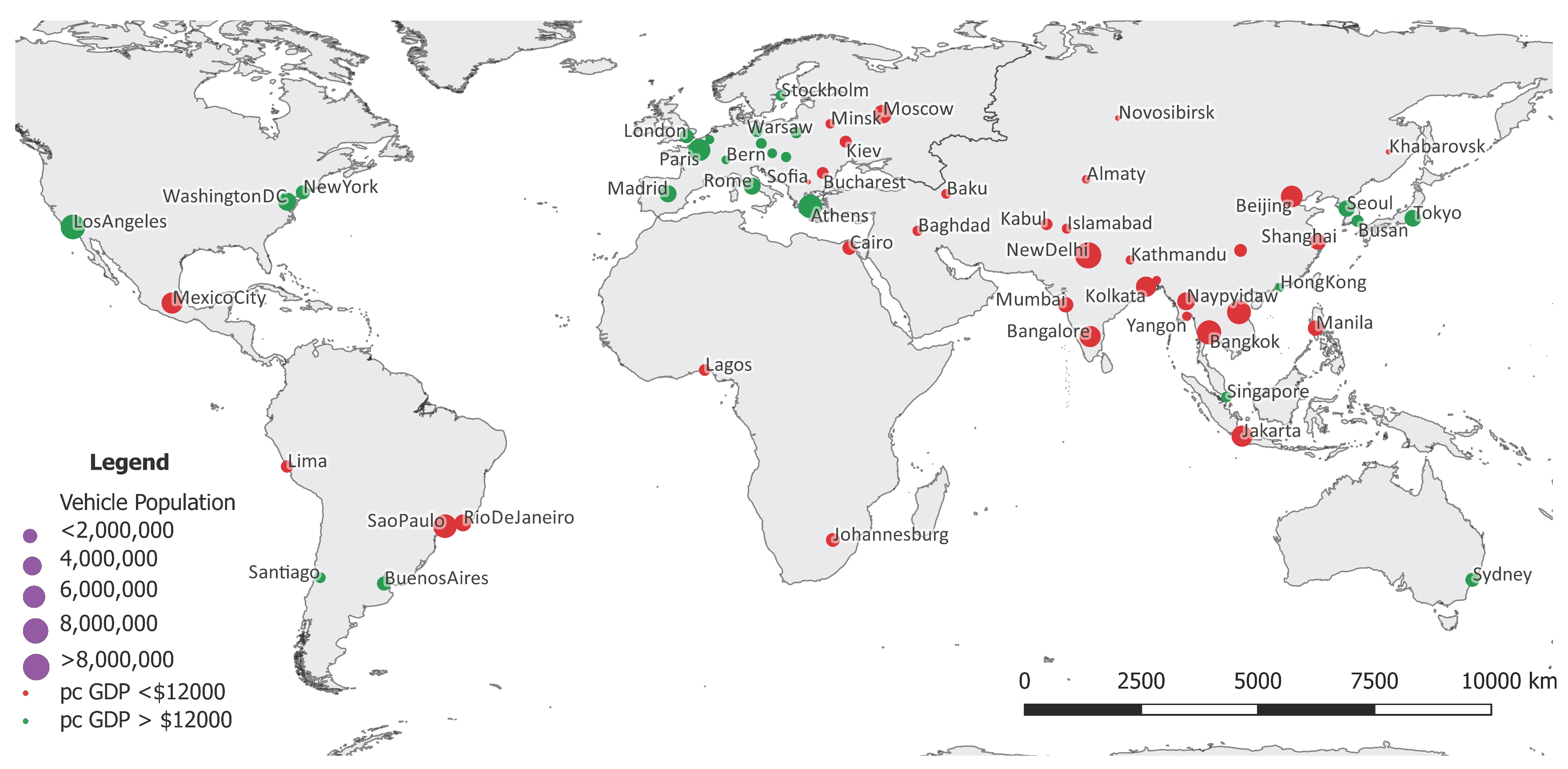
Figure 2.
Flowchart of study outlining data, processing and analysis. AOD and ANG refer to the aerosol optical depth and Angstrom exponent products respectively.
Figure 2.
Flowchart of study outlining data, processing and analysis. AOD and ANG refer to the aerosol optical depth and Angstrom exponent products respectively.

Figure 3.
Finding (distance metric corresponding to vertex G) for a point C lying within bounding . The vertices and B refer to scenarios of (a) high and AOD, (b) high and low AOD and, (c) low and low AOD. In this figure, is the absolute sum of areas of dotted rectangle () and hatched rectangles () (Equation (3)). Note that, since , will effectively be the difference of the areas of rectangles, will decrease towards zero as C approaches any vertex other than G.
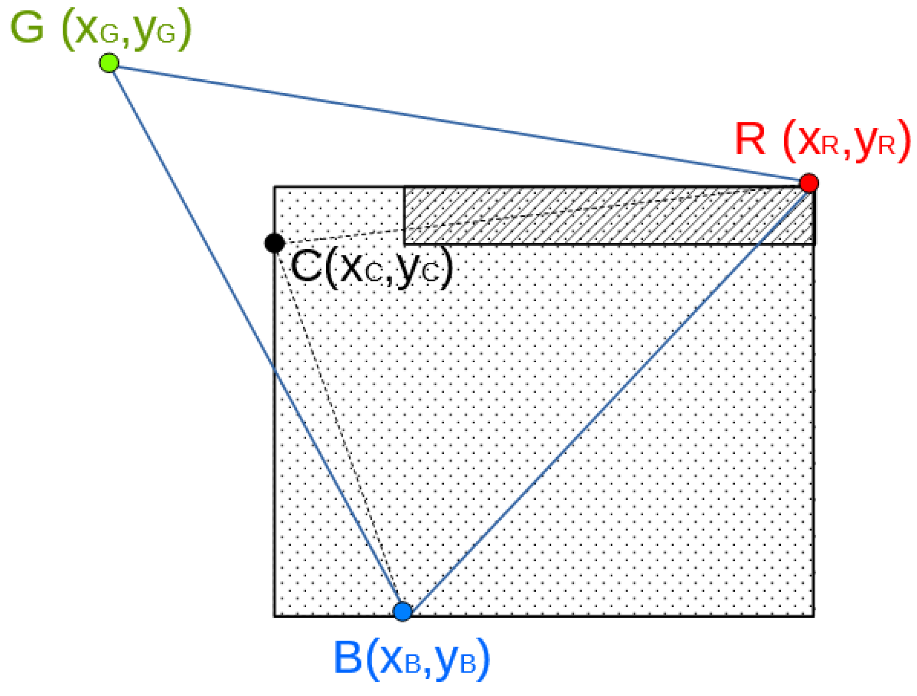
Figure 4.
Scatter plot of mean of monthly aerosol optical depth (AOD) and Angstrom exponent, (ANG) value of each city under study. The corresponding standard deviations are depicted as horizontal and vertical lines. Cities for which availability of valid data is less than 100 months are shaded light (e.g., Lagos, Singapore). This figure also shows the bounding triangle, with each vertex corresponding to extreme scenarios of aerosol optical depth and Angstrom exponent value, and are labeled as R, G and B.

Figure 5.
Proposed AirRGB scale for transformation based on bounding triangle shown as a three-band RGB image. On this scale, proximity to a vertex results in a higher value of the color corresponding to that vertex.
Figure 5.
Proposed AirRGB scale for transformation based on bounding triangle shown as a three-band RGB image. On this scale, proximity to a vertex results in a higher value of the color corresponding to that vertex.

Figure 6.
Global visualization of AirRGB using mean annual datasets of 2001, 2005, 2010 and 2015. Over this period, industrial regions across North India tend towards more intense R while Eastern China shows a decrease in intensity of R after year 2010.
Figure 6.
Global visualization of AirRGB using mean annual datasets of 2001, 2005, 2010 and 2015. Over this period, industrial regions across North India tend towards more intense R while Eastern China shows a decrease in intensity of R after year 2010.
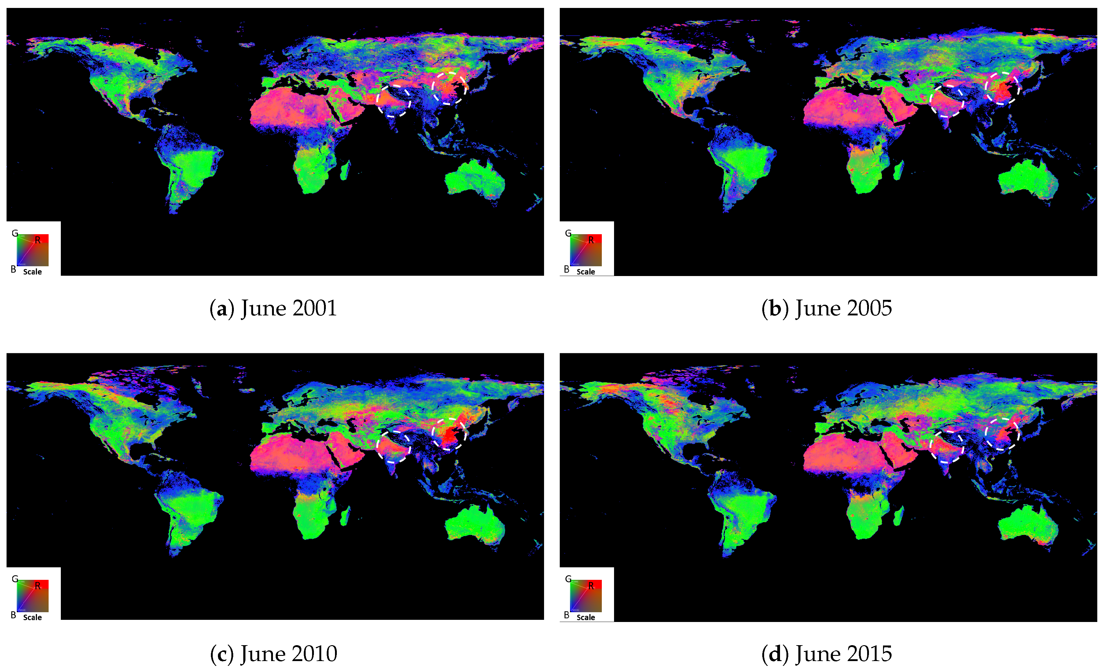
Figure 7.
Comparison of AirRGB trend of offset and slope for cities with extreme RGB values (New Delhi, Manila and Madrid) and other Asian cities (Beijing, Tokyo and Dhaka) over a period from January 2001 to December 2016. Values of R, G, B components are presented as a four-month moving average to ease visual interpretation.


Figure 8.
Global comparison of slope and offset for monthly R, G, B components of AirRGB trend from January 2001 to December 2016. Clusters of cities are separated by a dashed line in (a,b), while outlying locations in (a,c) are denoted within a dotted ellipse.
Figure 8.
Global comparison of slope and offset for monthly R, G, B components of AirRGB trend from January 2001 to December 2016. Clusters of cities are separated by a dashed line in (a,b), while outlying locations in (a,c) are denoted within a dotted ellipse.

Figure 9.
Scatter plot of AirRGB values versus PM2.5 observations. Whenever R reaches 100, G and B reach zero.
Figure 9.
Scatter plot of AirRGB values versus PM2.5 observations. Whenever R reaches 100, G and B reach zero.


Table 1.
Mean values of PM2.5, R, G and B.
| PM2.5 Range (g/m) | Count | Mean PM2.5 (g/m) | Mean R | Mean G | Mean B |
|---|---|---|---|---|---|
| 0–25 | 301 | 13.72 | 13.12 | 60.16 | 26.7 |
| 26–50 | 196 | 36.7 | 29.79 | 44.7 | 25.49 |
| 51–75 | 129 | 61.79 | 51.93 | 30.26 | 17.79 |
| 76–100 | 97 | 86.72 | 64.62 | 20.93 | 14.44 |
| 101–125 | 61 | 111.72 | 74.68 | 16.2 | 9.11 |
| 126–150 | 66 | 137.59 | 80.78 | 10.57 | 8.64 |
| 151–175 | 37 | 161.91 | 88.04 | 6.88 | 5.06 |
| 176–200 | 25 | 189.48 | 95.47 | 2.13 | 2.38 |
© 2017 by the authors. Licensee MDPI, Basel, Switzerland. This article is an open access article distributed under the terms and conditions of the Creative Commons Attribution (CC BY) license (http://creativecommons.org/licenses/by/4.0/).
Share and Cite
MDPI and ACS Style
Misra, P.; Fujikawa, A.; Takeuchi, W. Novel Decomposition Scheme for Characterizing Urban Air Quality with MODIS. Remote Sens. 2017, 9, 812. https://doi.org/10.3390/rs9080812
AMA Style
Misra P, Fujikawa A, Takeuchi W. Novel Decomposition Scheme for Characterizing Urban Air Quality with MODIS. Remote Sensing. 2017; 9(8):812. https://doi.org/10.3390/rs9080812
Chicago/Turabian StyleMisra, Prakhar, Aya Fujikawa, and Wataru Takeuchi. 2017. "Novel Decomposition Scheme for Characterizing Urban Air Quality with MODIS" Remote Sensing 9, no. 8: 812. https://doi.org/10.3390/rs9080812
Note that from the first issue of 2016, this journal uses article numbers instead of page numbers. See further details here.