Article

Sea State Observation through a Three-Antenna Hybrid XT/AT InSAR Configuration: A Preliminary Study Based on the InSAeS4 Airborne System

1
Istituto per il Rilevamento Elettromagnetico dell’Ambiente (IREA)—Consiglio Nazionale delle Ricerche (CNR), 80124 Napoli, Italy
2
Dipartimento di Ingegneria (DI), Università degli Studi di Napoli “Parthenope”, 80143 Napoli, Italy
*
Author to whom correspondence should be addressed.
Remote Sens. 2017, 9(8), 792; https://doi.org/10.3390/rs9080792
Submission received: 28 April 2017 / Revised: 30 June 2017 / Accepted: 28 July 2017 / Published: 1 August 2017
(This article belongs to the Special Issue Radar Systems for the Societal Challenges)

Abstract

:
In this work, we investigate the sea surface monitoring capabilities of a Synthetic Aperture Radar (SAR) system equipped with a three-antenna hybrid Across Track (XT)/Along Track (AT) inteferometric configuration. To do this, we focus on the X-Band airborne InSAeS4 SAR system. Moreover, we propose a simple but effective methodology that allows simultaneous retrieval of the sea surface height and velocity by means of a straightforward, easy-to-implement, linear inversion procedure, which is very general and can be implemented with any system equipped with a three-antenna hybrid XT/AT Interferometric SAR (InSAR) configuration. In our case, we present an experiment carried out in January 2013 in South Italy over the coastline stretch of the Campania region including the Volturno River outlet. In this regard, we highlight that in situ measurements of the retrieved sea surface height and velocity at the time of the airborne mission are unfortunately not available. Notwithstanding, the obtained results show some interesting evidence that the estimated quantities are physically sound. This, on the one side, provides a preliminary validation of the effectiveness of the overall presented methodology and, on the other side, highlights the potentialities of the three-antenna hybrid XT/AT InSAR configuration of the InSAeS4 system for sea state monitoring.

Graphical Abstract

1. Introduction

Synthetic Aperture Radar (SAR) is a microwave remote sensing sensor that can be mounted on spaceborne platforms [1,2], airplanes [1,2], helicopters [3], drones [4], cars [5] and ground stations [6,7], and allows all-weather, night and day imaging of the illuminated area. In particular, exploitation of the phase difference, named interferogram, between focused SAR data pairs acquired by antennas that illuminate the same area from different positions and/or at different times makes it possible to obtain key information on the observed scene [1,2,8,9] through the so-called SAR Interferometry (InSAR) technique.
More specifically, if two SAR antennas are simultaneously present and displaced along the across-track (XT) plane, that is, the direction orthogonal to the radar flight one, the corresponding interferogram is sensitive to the topography of the illuminated area [1,2,10]. In this case, the interferometric technique is referred to as XT-InSAR, and allows us to generate a Digital Elevation Model (DEM) of the observed scene. In fact, an XT-InSAR configuration can be obtained either with a single pass of a multiple antenna system or with repeat passes of a single antenna system.
If two SAR antennas are instead displaced along the radar flight track, the SAR data relevant to the same target are acquired by the different antennas with a short time lag. Accordingly, for each illuminated target, the interferogram is sensitive to the changes (if any) of the sensor-to-target distance occurred during this time lag [11,12]. In this case, the interferometric technique is referred to as Along Track InSAR, briefly AT-InSAR, and allows us to monitor fast-varying phenomena occurring in the observed area, such as those related to currents and waves in marine scenarios [11,12,13,14,15,16] or to the vehicle fluxes in marine as well as land scenarios [17].
Finally, if the antennas are displaced along both the XT and AT directions, the corresponding interferogram is sensitive to both the topography of the illuminated scene as well as the fast-varying phenomena occurred in the time interval elapsed between the different acquisitions carried out by the different antennas. Accordingly, exploitation of a hybrid XT/AT InSAR configuration in marine scenarios involves advanced remote sensing features, because it allows simultaneous retrieval of both the height profile and the velocity of the observed sea surface. Of course, this entails the application of a proper data processing strategy aimed at separating the XT contribution (which is sensitive to the sea surface height) from the AT one (which is sensitive to the sea surface velocity), both present in the obtained interferogram. This task is however not straightforward, and needs to be carefully addressed.
In particular, if a two-antenna hybrid XT/AT InSAR configuration is available, some assumptions on the nature of the observed scene must be necessarily done. For instance, in the airborne experiment in [18] two antiparallel acquisitions were carried out with a time delay of 10 min. In this way, two different single-pass interferograms relevant to the same scene and acquired at different times were collected. Under the assumption that the sea conditions did not change between the repeated passes of the airplane, proper combination of these two single-pass interferograms allowed retrieving the searched XT and AT contributions. However, especially in marine scenarios characterized by strong currents and waves, the assumption that the sea conditions do not significantly change in the time span elapsed between the repeated radar passes may be not well satisfied, even with an airborne platform, which generally allows keeping quite small the time lag between the different flight tracks.
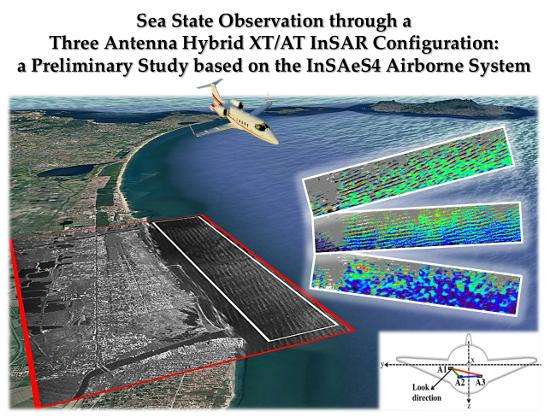
To overcome this problem, we exploit in this work the three-antenna hybrid XT/AT InSAR configuration of the airborne X-Band InSAeS4 SAR system [19]. Moreover, we propose a simple but effective methodology that allows simultaneous retrieval of the sea surface height and velocity by means of a straightforward, easy-to-implement, linear inversion procedure. Indeed, due to the availability of a three-antenna hybrid XT/AT InSAR configuration, it is possible to acquire, simultaneously, two independent interferograms containing the same information about the height and the velocity of the illuminated sea surface. This makes it possible the straightforward separation of the XT and the AT contributions present in the two interferograms, thus allowing us to jointly estimate, on a pixel-by-pixel basis, the velocity and height of the illuminated marine scene.
The proposed methodology, which is very general and can be implemented with any system equipped with a three-antenna hybrid XT/AT InSAR configuration, has been here applied to an interferometric data-set acquired on January 2013 by the InSAeS4 SAR system along the coastline stretch of the Campania region, South of Italy, over the Volturno River.
The work is organized as follows. In Section 2, we provide a brief description of the InSAeS4 system. In Section 3, we present the main rationale of the algorithm that carries out the separation of the XT and AT contributions by exploiting a couple of independent interferograms acquired by a three-antenna hybrid XT/AT InSAR system. The experimental results are shown in Section 4. Section 5 is devoted to the concluding remarks.

2. System Description

InSAeS4 [19], also named TELAER [20], is an Italian interferometric airborne SAR system operating at X-Band. The system is equipped with a hybrid XT/AT InSAR configuration consisting of three antennas installed onboard in such a way to allow the simultaneous presence of three AT baseline components (which, in the absence of pitch and yaw, are equal to 0.56 m, 0.21 m and 0.35 m, respectively), and three XT baseline components (which, in the absence of pitch and yaw, are equal to 0.76 m, 0.93 m and 1.59 m, respectively). For the sake of clearness, the antenna layout is depicted in Figure 1.
The system is installed onboard a Learjet 35A, whose main parameters are collected in Table 1. An extended description of the InSAeS4 system can be found in [19]. Here we report the main radar parameters, see Table 2, and recall that the radar is equipped with a single transmitter; accordingly, for two (of the three available) interferometric channels, the system operates in bistatic mode. Moreover, we remark that this radar system is quite flexible, in the sense that it is able to transmit signals with a bandwidth ranging from 50 MHz to 400 MHz, with an effective (ground) range swath ranging from 2 km to about 6 km (depending on the bandwidth of the transmitted signal as well as on the number of activated interferometric channels). For instance, the widest bandwidth (400 MHz) is coupled with the narrowest swath and allows reaching the highest geometric resolution, that is, 50 cm (slant range) × 15 cm (azimuth) (see [19] for further details).
In [19], a first assessment of the XT-InSAR system capabilities is provided. In particular, to neglect the AT-InSAR contribution in the interferograms obtained with the hybrid XT/AT InSAR configuration of the system, in [19] we have analyzed a data-set acquired over a land area. By doing so, with the 400 MHz mode and with the longest (orthogonal) baseline data pair, we have generated a single-pass DEM characterized by a mean vertical error of few centimeters and standard deviation of half meter on corner reflectors and one meter and half over open terrain.
A detailed analysis on the AT-InSAR capabilities of the system, not addressed in [19], is carried out in the following sections.

3. Rationale of the Proposed Methodology

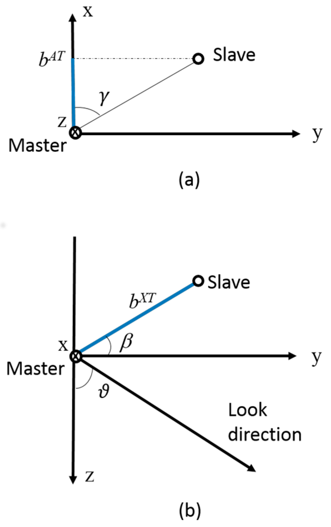
Let us consider a three-antenna hybrid XT/AT InSAR configuration, such as (but not necessarily equal to) that depicted in Figure 1. Following the figure notation, the three antennas are named Ai, i {1, 2, 3}, and the corresponding interferometric channels are named 1, 2 and 3, respectively.
In the following, for the sake of generality, we will consider the airborne SAR case, thus assuming the sensor velocity and the squint angle not constant during the acquisition. In this regard, we underline that the output SAR grid is chosen hereafter with respect to a nominal one, that is rectilinear, representing the reference track relevant to the actual master track [21]. Accordingly, in the following, the azimuth direction is coincident with such nominal direction. Moreover, for sake of simplicity, the mean squint angle during the acquisition is assumed to be zero. Anyway, extension to (on average) squinted acquisitions will be discussed at the end of this section.
Let us consider a marine scenario and denote with ∆ϕij the interferogram obtained with the interferometric channels i and j, being i the master channel and j the slave one, respectively. It is assumed that the interferogram ∆ϕij has been flattened (i.e., the topographic contribution provided by an available, even low accuracy, external DEM, such as the SRTM [22] one, has been removed) and unwrapped [1]. Moreover, it is also assumed that the constant phase offset introduced in the interferogram by the phase unwrapping procedure has been properly removed [23]. In the most general case, that is, when both the XT and AT baseline components are present in the considered interferometric pair, ∆ϕij is sensitive to both the topography of the illuminated area and the fast-varying phenomena therein occurred between the different acquisitions carried out by the different antennas. Accordingly, for each pixel of such interferogram it possible to write:
Δ ϕ i j α i j Δ z + η i j u r
where ∆z is the difference between the vertical height of the considered target and the reference vertical height provided by the external DEM exploited to flatten the interferograms, and ur is the Line-Of-Sight (LOS) component of the target velocity. More specifically, in a marine scenario, ur is the sum of three contributions: the LOS components of the orbital motion of water particles from the swell, the phase velocity of the Bragg waves and any underlying ocean currents that may exist [11]. Moreover, the expressions of the coefficients αij and ηij in Equation (1) can be found in [1,11], respectively, and are reported in the following:
α i j ( x , r ) = d 2 π b i j ( x , r ) λ r sin ϑ ( x , r )
η i j ( x ) = d 2 π b i j A T ( x ) λ V x ( x )
where x and r are the azimuth and range coordinates, respectively, of the considered pixel. Furthermore, in Equations (2) and (3), as usual, the subscripts i and j denote the interferometric channels relevant to corresponding interferogram; λ is the wavelength of the carrier signal and the coefficient d depends on the exploited interferometric configuration (d = 1 for bistatic systems, whereas d = 2 for monostatic ones). Moreover, in Equation (2) ϑ(x, r) is the look angle, b i j ( x , r ) is the so called orthogonal baseline [1,10] (which depends, in turn, on the XT baseline component and the look angle ϑ(x, r), see [1]). Finally, in Equation (3) b i j A T ( x ) is the AT baseline component (defined as the difference between the azimuth coordinates of the antennas i and j) and V x ( x ) is the azimuth component of the aircraft velocity. It is stressed that, according to the notation adopted in Equations (1)–(3), when a generic observed target recedes from the radar the radial velocity ur in Equation (1) is negative. It is also remarked that, due to the aircraft attitude variations, the quantity b i j A T changes (although very marginally) during the acquisition. In this regard, it is also noted that in the satellite case, where the sensor tracks are very stable, both b i j A T and V x can be safely assumed constant during the flight, thus rendering the coefficient η i j in Equation (3) constant as well in the overall interferogram.
When a three-antenna hybrid XT/AT InSAR configuration is used, two independent interferograms are available. Therefore, according to Equation (1), for each pixel it is possible to build a linear system of two equations in two unknowns:
Δ = M ν
where Δ = [ Δ φ i j , Δ φ i k ] i , j , k { 1 , 2 , 3 } , i j k T collects the two available interferograms, ν = [ Δ z , u r ] T collects the two unknowns and M = [ α i j η i j α i k η i k ] . It is worth highlighting that the system in Equation (4) is linear due to the approximations adopted in Equation (1). On the other side, as shown now in the following, such approximations are often appropriate.
More specifically, with reference to the XT InSAR contribution, we have considered in Equation (2) the well-known linear Taylor’s expansion of the (nonlinear) operator that carries out the phase-to-height conversion [1,10]. Such an approximation can be safely applied in a marine scenario where the height of the sea surface (that is, the amount of ∆z in Equation (1)) is expected to be at most on the order of some meters.
Moreover, in Equation (1), it has been neglected the non-linear term that arises when observing a moving target with an InSAR data pair characterized by a non zero XT baseline component. To better clarify this point, we recall that:
(i).
The SAR impulse response of a target moving with radial velocity ur is affected by an azimuth shift equal to u r r / V x [16] and an azimuth phase ramp whose rate γ is equal to d 2 π λ u r V x [24].
(ii).
In an InSAR data pair separated by an XT baseline component, the same (even steady) target is located at two different range coordinates [1] ri and rj (where, as usual, i denotes the master channel and j the slave one) differing by an amount δrij = rj − ri.
Accordingly, combining effects (i) and (ii) leads to the following azimuth misregistration term [18]:
δ x i j = δ r i j V x u r
and then to the following InSAR phase contribution
δ φ i j = γ δ x i j = d 2 π λ ( u r V x ) 2 δ r i j
As shown in Appendix A, in our experiment the extra-phase term in Equation (6) can be safely neglected in Equation (1).
Turning to the AT InSAR contribution, we have exploited in Equation (3) the same linear relation originally proposed in [11], thus neglecting the nonlinear effects discussed in [16] and related to the velocity bunching. With particular reference to the InSAeS4 system described in Section 2, such an approximation can be safely applied because the r/Vx ratio is quite small. Indeed, it ranges from about 50 s in near range to 65 s in the near to coast area of Figure 2, thus being on the same order of magnitude of that found in the X-Band airborne SAR experiment presented in [18] (50 s), where exploitation of the linear relation in Equation (3) rather than the exact one is safely adopted.
Summing up, under the conditions discussed above, with a three-antenna hybrid XT/AT InSAR configuration the separation of the XT and AT InSAR contributions from the available interferograms can be straightforwardly achieved, on a pixel-by-pixel basis, through the inversion of the linear system of two equations in two unknowns reported in Equation (4). In this regard, we note that different options involving the design of the three-antenna layout of a hybrid XT/AT InSAR configuration are possible in order to obtain a full rank system matrix M in Equation (4).
The first, obvious possibility is to deploy the three-antennas in such a way to render the diagonal elements of the matrix M in Equation (4) all equal to zero. This means that (in the absence of pitch and yaw) a couple of antennas are separated only by an XT baseline, whereas other two of them are separated only by an AT baseline. In this case, the two unknowns, namely ur and ∆z, are already separated in the two interferograms, thus rendering this layout particularly attractive in marine scenarios.
On the other side, in land scenarios, where one is interested in calculating only the DEM of the observed scene, such kind of layout cuts off the possibility of exploiting two different XT baseline components to improve the accuracy of the final InSAR DEM in regions characterized by steep topography [25]. For this reason, a more flexible solution, optimally tailored to land scenarios and well exploitable also over marine ones, is the one depicted in Figure 1, where the antennas are deployed in such a way to render all the coefficients of the matrix M in Equation (4) not equal to zero. Indeed, as stressed above, in this case separation of the XT and AT InSAR contributions, both present in the available interferograms, can be easily obtained just inverting the linear system in Equation (4).
Extension of the model in Equations (1)–(4) to squinted acquisitions is now discussed.
When considering a hybrid XT/AT InSAR configuration in the presence of a squint angle, say φs, the azimuth misregistration term in Equation (5) is responsible also for the following phase contribution:
δ φ i j = d 2 π λ sin ( ϕ s ) δ x i j = d 2 π λ V x sin ( ϕ s ) δ r i j u r
where use of Equation (5) has been done in the last equality of Equation (7). This extra phase term, however, does not act on the linearity of the system in Equation (4) and can be easily accounted for by still applying Equation (1), provided that the following substitution:
b i j A T ( x ) b i j A T δ r i j ( x , r ) sin ( φ s )
is done in Equation (3).
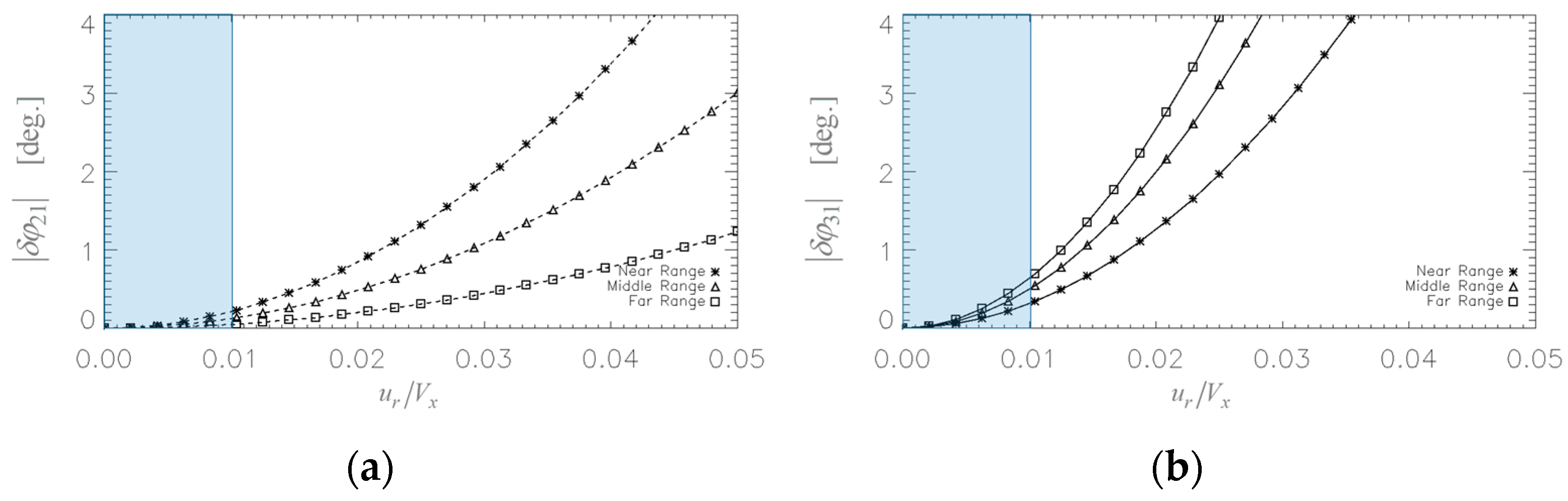
It is finally remarked that the unavoidable presence of errors in the calculation of the orthogonal baseline ( b ) and the AT baseline (bAT) may impair, at least in principle, the accuracy of the inversion of the linear system in Equation (4). However, as shown in Appendix B, in our experiment these effects can be safely neglected.

4. Experimental Results

In this section, we have applied the methodology presented in Section 3 to a real data-set acquired by the InSAeS4 system, exploiting its three-antenna hybrid XT/AT InSAR configuration depicted in Figure 1. The experiment is relevant to the test-flight campaign carried out during January 2013 along a coastline stretch of the Campania region, in the South of Italy, including the estuary of the Volturno River.
SAR data have been transmitted with 100 MHz bandwidth. Table 3 collects the main mission and data processing parameters. 
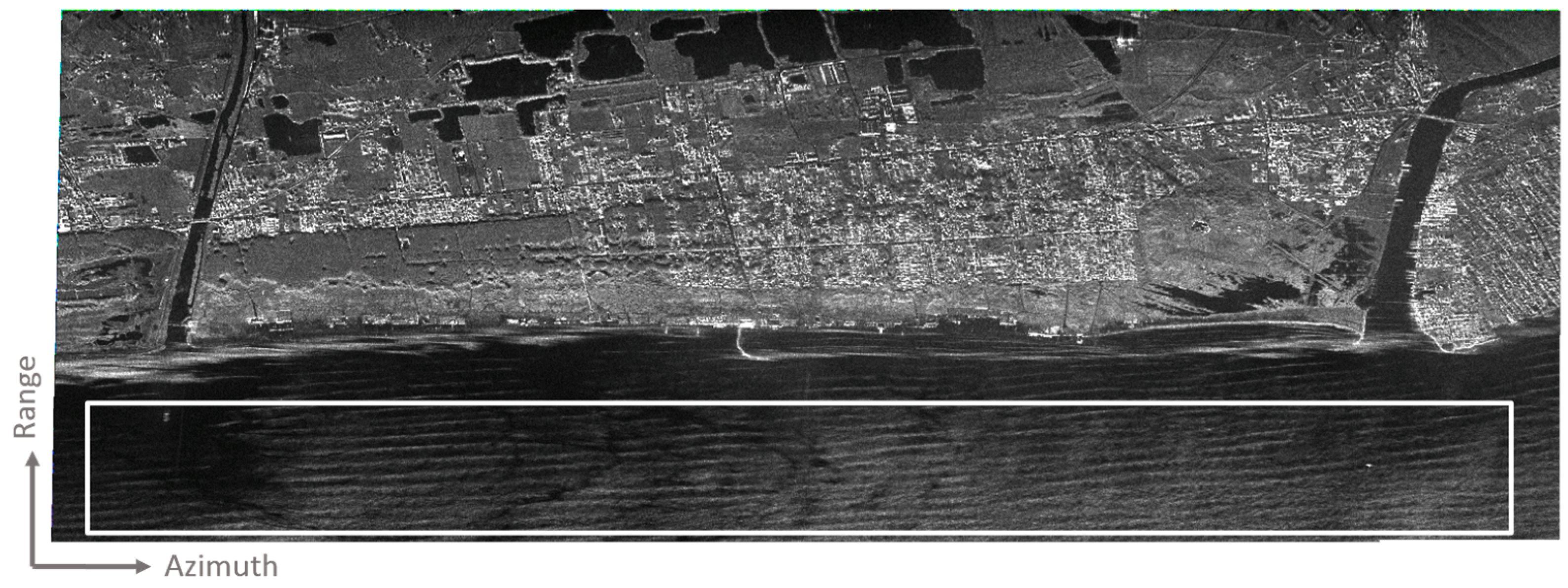
Figure 2 shows one of the three focused multi-look SAR images, where a 4 × 32 (range × azimuth) pixel averaging (leading to a resolution of 6 m in slant range and 5 m in azimuth) has been applied. As can be seen, the test area, which is about 7 km long and almost parallel to the coastline, includes both sea and land regions.
In order to solve the linear system in Equation (4), in this paper, we focus on the interferograms ∆ϕ21 and ∆ϕ31, where reference to Figure 1 has been done to denote the channels’ (antennas’) numbers. It is noted that one data pair (∆ϕ21) is characterized by the longest AT baseline component (which is coupled to the shortest XT baseline component) of the InSAR configuration of the system. The other data pair (∆ϕ31), instead, is characterized by the longest XT baseline component (which is coupled to the intermediate AT baseline component).
Along the lines shown in Section 3, as first step we have calculated the coefficients of the matrix M in Equation (4). In this regard, Figure 3a shows, for both data pairs, the corresponding AT baseline components as a function of the azimuth coordinates. From the reported plots, by considering the operating velocity of the Learjet 35A during the mission (see Table 3), we obtain mean unambiguous velocity values [11,12] equal to 11.5 m/s for the data pair 1–3 and 7.1 m/s for the data pair 1–2. Figure 3b shows, again for both data pairs, the corresponding orthogonal baselines as a function of the range coordinate. In this regard, it is recalled that the orthogonal baseline depends on both range and azimuth. In our case, however, the topographic profile of the illuminated area is quite smooth, thus leading to a very limited variation of the look angle along the azimuth direction. On the other side, as always happens in airborne acquisitions, the look angle shows a very large variation from near to far range (see Table 3). Therefore, the azimuth variations of the orthogonal baseline are negligible with respect to the range ones. In any case, in Figure 3b, for each range coordinate, we have reported the mean value of the orthogonal baseline respect to the azimuth samples. From the reported plots, by considering the flight parameters of Table 3, we obtain a height of ambiguity [1] value that ranges from 58 m to 180 m in the data pair 1–3, and from 121 m to 300 m for the data pair 1–2.
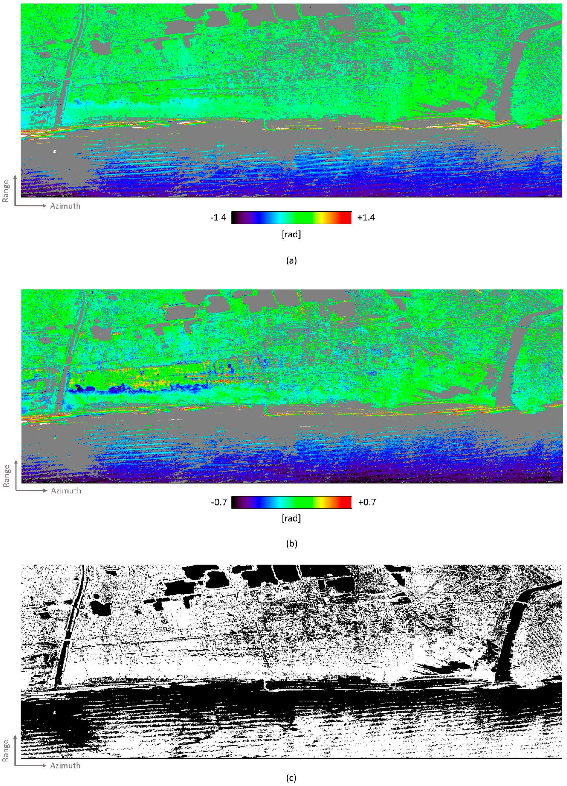
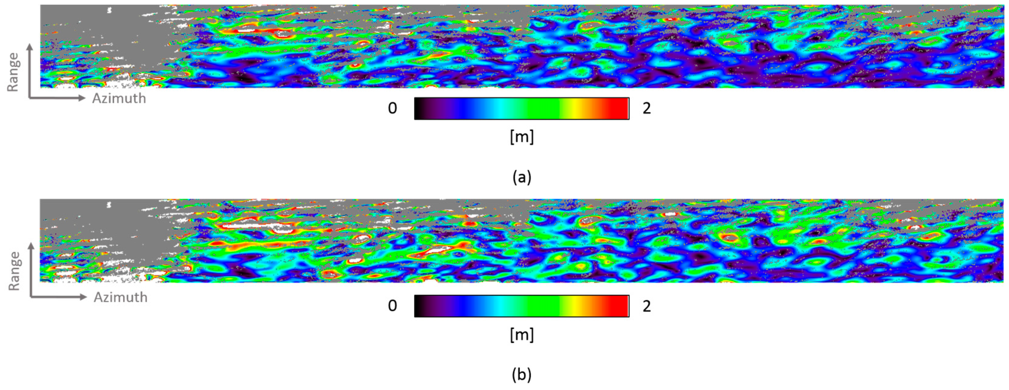
Figure 4a,b shows the two interferograms ∆ϕ21 and ∆ϕ31. It is highlighted that, in the shown figures, we have considered the same multi-look factors as Figure 2 (leading to a resolution of 6 m in slant range and 5 m in azimuth); however, the inversion in Equation (4) has been carried out on higher resolution data (with resolution equal to 1.5 m in slant range and 0.6 m in azimuth). Moreover, as explained in Section 3, both interferograms have been flattened and unwrapped [1].
In particular, the former operation has been carried out by exploiting the SRTM DEM [22]. Such DEM has been used also to carry out the motion compensation procedure during the SAR focusing step [21], and to estimate and remove the unknown phase offset value affecting the interferograms after the application of the unwrapping procedure [26]. Note that in both figures we have masked (with the gray color) the pixels whose InSAR coherence [1] value is smaller than 0.7 at least in one of the two interferograms. The adopted coherence mask is shown in Figure 4c. It can be observed that, in both interferograms, wide areas of the considered sea region exhibit high coherence along the whole sea wave profiles (that is, from the crests to the troughs).
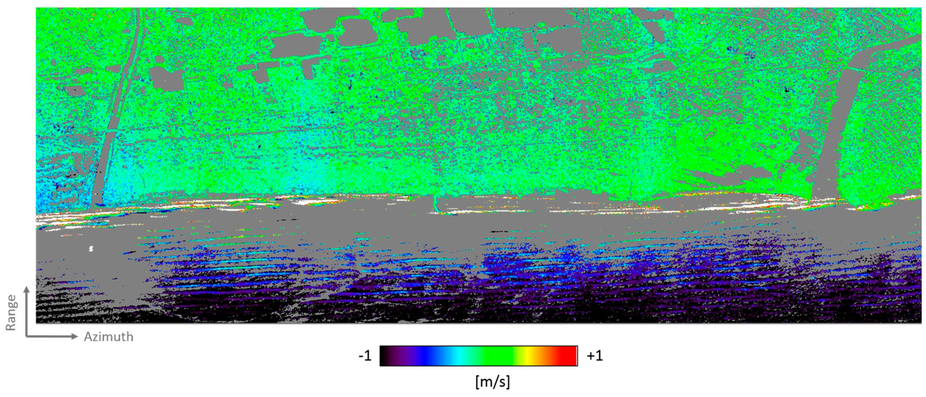
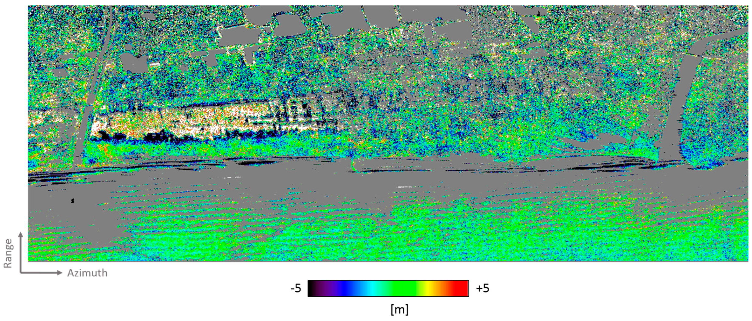
By inverting the system in Equation (4), we have obtained the surface height ( Δ z ^ ) and velocity ( u ^ r ) maps reported in Figure 5 and Figure 6, respectively. In both maps, we have masked the pixels whose interferometric coherence value is smaller than 0.7 at least in one of the two interferograms of Figure 4. Moreover, the maps, which have been obtained at 1.5 m (range) × 0.6 m (azimuth) resolution, are shown in the figure at the same resolution as that of the data reported in Figure 2 and Figure 4.
Although precise information on the ground truth provided by buoys or similar instruments is not available, the obtained results show some interesting evidence of the effectiveness of the presented procedure.
First, in Figure 6, we can see that the estimated radial velocity u ^ r turns out to be approximately zero in correspondence of the land region. This of course represents a good first order check of the effectiveness of the proposed procedure in separating the XT and AT contributions occurring in the interferograms generated through the considered three-antenna hybrid XT/AT InSAR system.
Turning to the estimated surface height map Δ z ^ shown in Figure 5, we stress once again that it represents the difference between the vertical height provided by the SRTM DEM (which has been used to flatten our interferograms) and that achieved with our InSAR configuration. In particular, over the land region, the topographic map of Figure 5 highlights the difference between the vertical accuracy of the SRTM DEM and the DEM achievable with the InSAeS4 system, whose topographic mapping capabilities have been previously discussed in [19]. Over the sea region, instead, the topographic map of Figure 5 represents the height of the illuminated sea surface, since over such region the topographic height provided by SRTM is constant and equal to zero. In this regard, it is stressed that Δ z ^ must not be confused with the true wave height (which is instead related to the difference between the crests and the troughs).
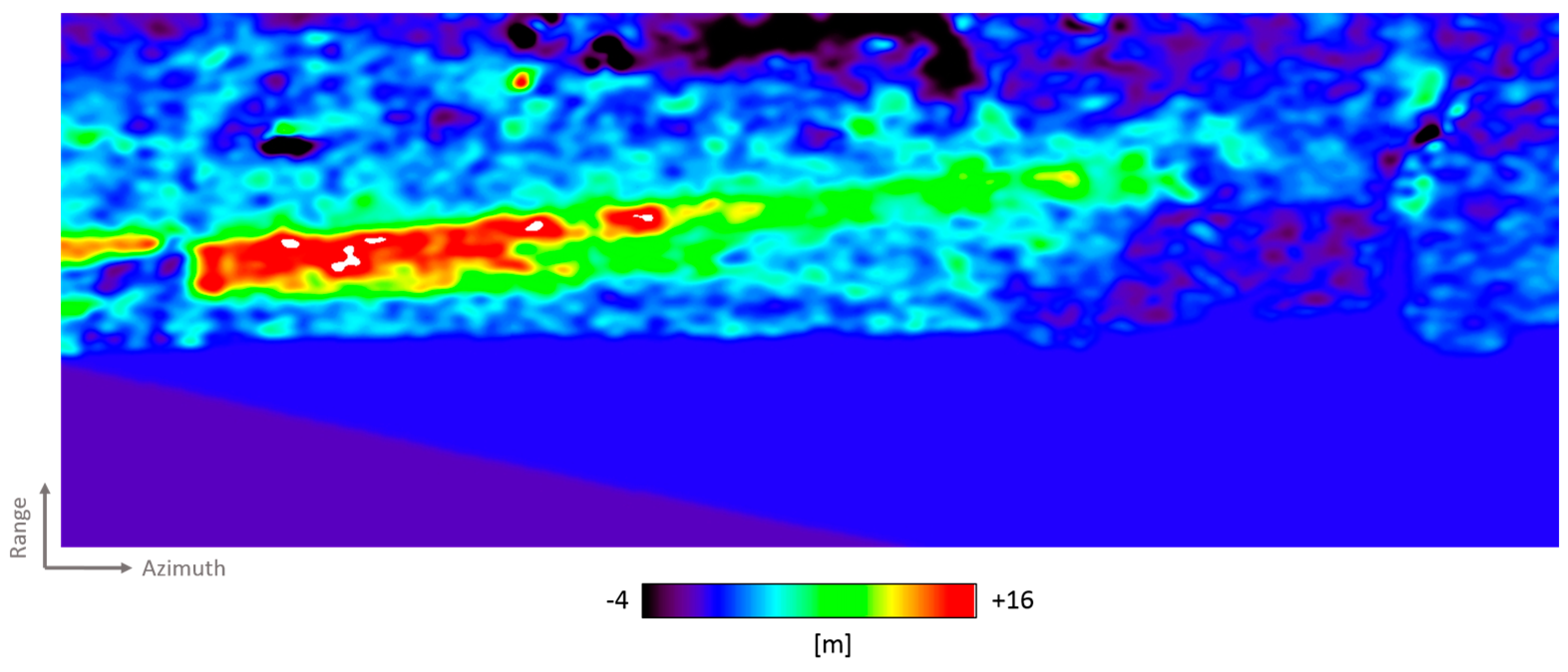
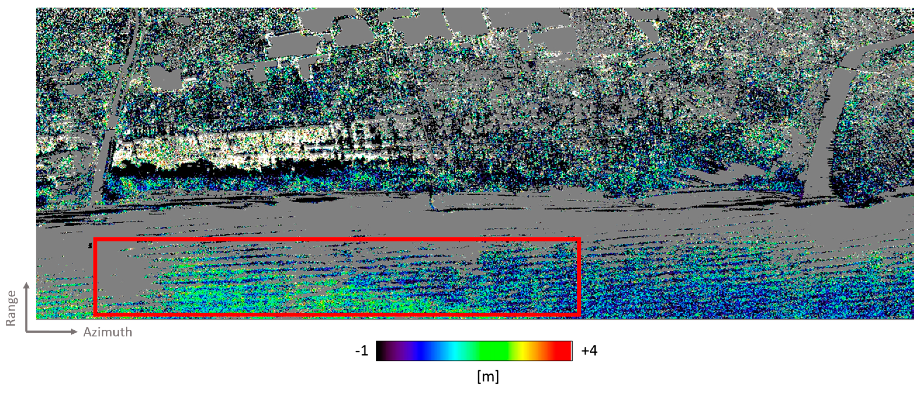
To provide a better insight on the effectiveness of the proposed approach in estimating the vertical profile of the illuminated sea waves, we have carried the following experiment. First, we have deliberately introduced a vertical bias of 1 m in the SRTM DEM in correspondence of a small portion of the illuminated sea area. The so obtained vertical profile, which is shown in Figure 7 in radar coordinates, has been then exploited to flatten our interferograms. Finally, we have applied the procedure of Section 3 to the so achieved interferograms. By doing so, we have obtained the surface height map Δ z ^ shown in Figure 8.
As can be seen, the 1 m step on the bottom-left corner of Figure 7 can be appreciated also in the surface height map Δ z ^ of Figure 8. To quantify this effect, within the obtained Δ z ^ map we have selected the rectangular region highlighted in red in Figure 8. Within this region, we have calculated the mean value of Δ z ^ in the top-right triangular region (where the vertical height of the reference DEM used to flatten the interferogram is 0 m, see Figure 7) and in the bottom-left triangular region (where the vertical height of the reference DEM used to flatten the interferogram is −1 m, see Figure 7). The difference between the so obtained values turned out to be equal to 1.14 m: the 1 m step in Figure 7 has been thus correctly retrieved in the map of Figure 8. Once again, the obtained results confirm the effectiveness of the overall methodology proposed to separate the XT and the AT contributions in the interferograms generated through the considered three-antenna hybrid XT/AT InSAR system. Moreover, this experiment shows that a vertical bias induced by tides on the external DEM relevant to the sea region does not affect significantly the capability of the presented procedure in separating the XT and the AT contributions from the interferograms.
Turning back to the results of Figure 5 and Figure 6, to improve the estimates obtained over the sea area, a filtering procedure has been applied to the Δ z ^ and u ^ r maps within the Region of Interest (RoI) highlighted with the white rectangle in Figure 2. In particular, since the considered RoI is relevant to a coastal region (see Figure 2), where the variability of the sea depth involves a spatial inhomogeneity of the sea wave features, an adaptive filtering procedure has been exploited. More specifically, for both maps we have performed a band pass filtering driven by the local properties of the quantities to be filtered. To this aim, we have split the RoI into a number of partly overlapping patches and tailored the filters according to the spectral properties of Δ z ^ and u ^ r 
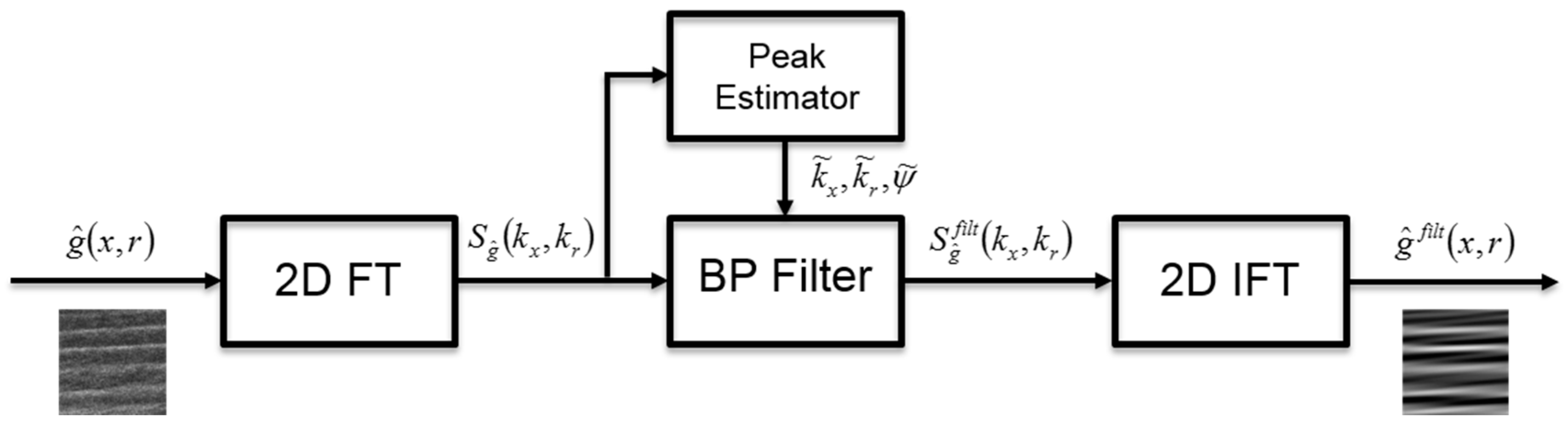
restricted to each patch. Finally, we have combined the so obtained filtered quantities by means of a mosaicking procedure. Some further considerations on the patch dimensioning and filtering are now needed.
Broadly speaking, the patch size must be large enough to allow a reliable spectral resolution but, at the same time, small enough to preserve as much as possible the space stationarity of the observed sea parameters. Moreover, enlarging the overlap between adjacent patches reduces the discontinuities of the filtered quantities at expenses of an increased computational burden of the overall procedure. According to these considerations we have set a patch size of about 384 m in range × 320 m in azimuth, with an overlap percentage of about 80% (with respect to the patch sizes). By doing so, we have covered the RoI with 1376 patches (16 along the range direction and 86 along the azimuth one).
As for the filtering procedure, for each patch we have first computed the 2D power spectra of u ^ r and Δ z ^ , say S u ^ r ( k x , k r ) and S Δ z ^ ( k x , k r ) , where kx and kr are the wavenumbers relevant to the azimuth and range directions, respectively.
Then, for each spectrum we have retrieved the dominant components, say ( k x u r , k r u r ) and ( k x Δ z , k r Δ z ) , and in turn the corresponding dominant propagation directions, say ψ u r = arctan ( k x u r / k r u r ) and ψ Δ z = arctan ( k x Δ z / k r Δ z ) , respectively. These values have been used to build two bivariate raised cosine band pass filters (whose complete expression is reported in Appendix C) to be applied to S u ^ r ( k x , k r ) and S Δ z ^ ( k x , k r ) , respectively. The block diagram of the patch filtering procedure is reported in Figure 9.
It is finally remarked that since the filtering procedure works in the spectral domain, it provides accurate results only if it can operate on coherent InSAR phases along the whole sea wave profiles (that is, from the crests to the troughs). As discussed above, in our case, this condition is well satisfied for both the exploited interferograms.
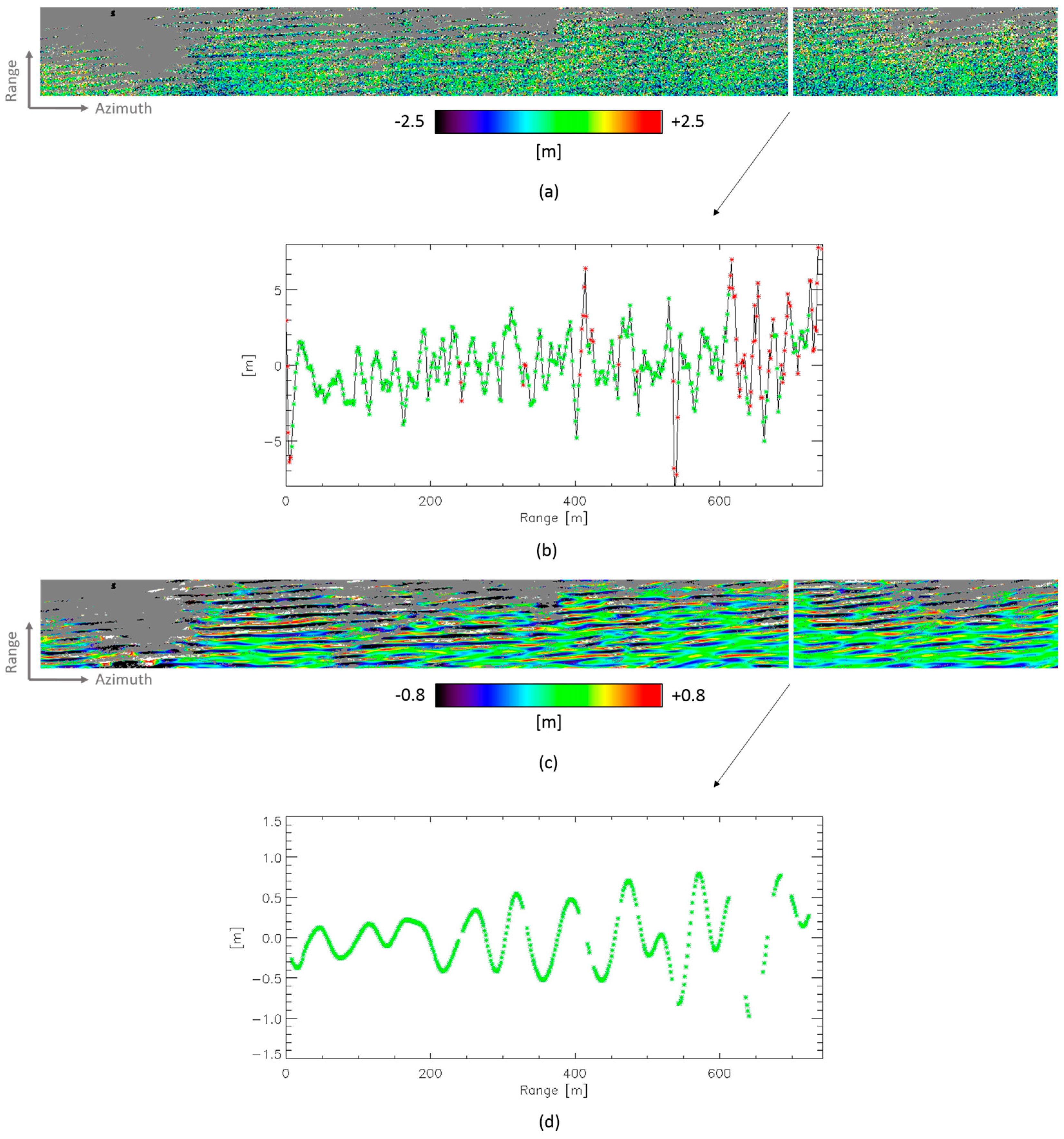
Figure 10 and Figure 11 show the estimated sea surface height and velocity maps, respectively, before (Figure 10a and Figure 11a) and after (Figure 10c and Figure 11c) the application of the filtering procedure. In both the filtered maps, say Δ z ^ f i l t and u ^ r f i l t , the features of the sea waves, which move toward the coastline along a direction very close to the range one, are clearly visible. As usual, in all maps, we have superimposed the mask of Figure 4c, that is, we have masked the pixels whose interferometric coherence value is smaller than 0.7 at least in one of the two interferograms of Figure 4.
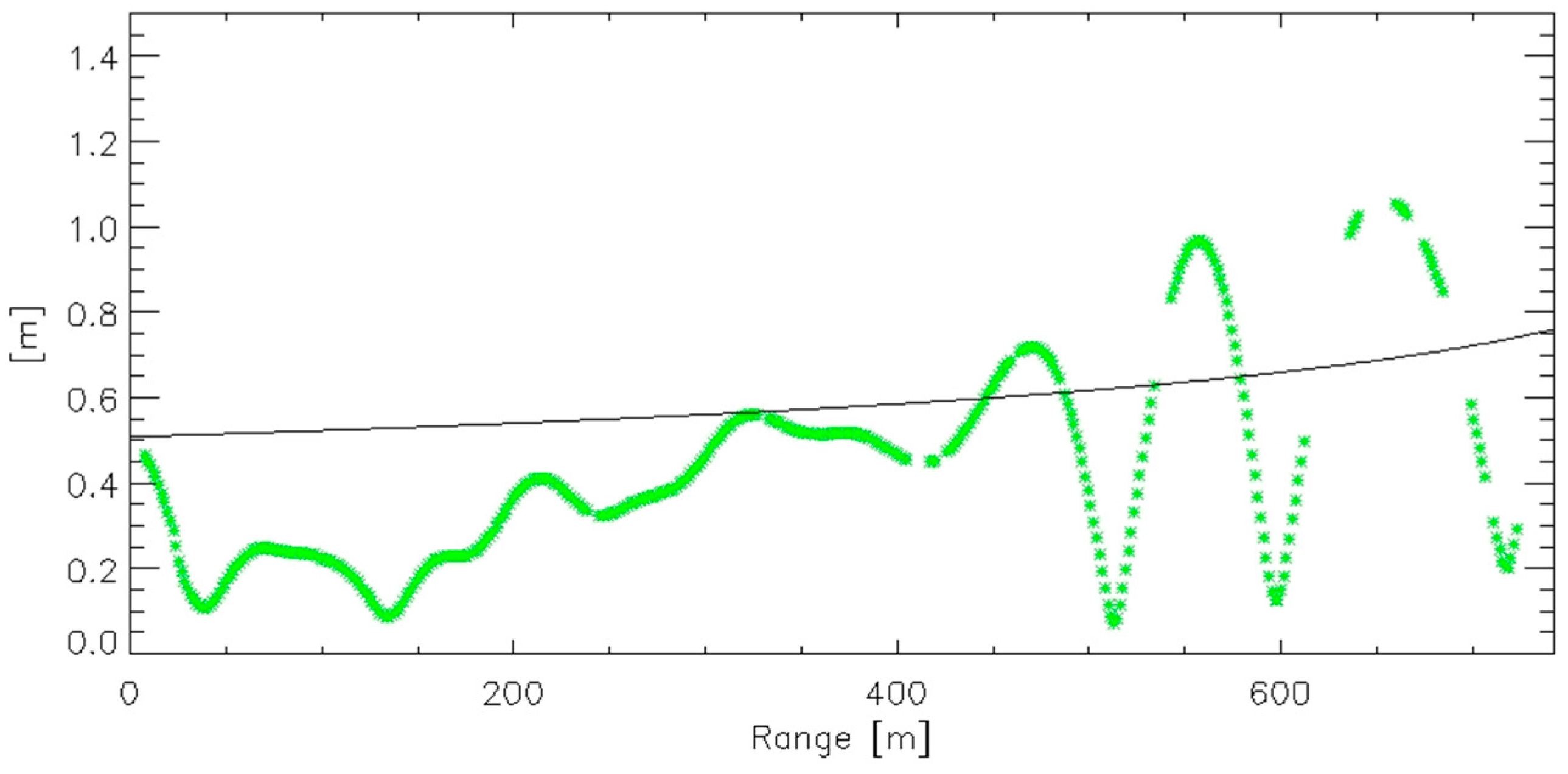
Let us concentrate on the sea surface height maps of Figure 10. For both maps, we have focused on the range cut highlighted in white in Figure 10a,c. The corresponding plots are reported in Figure 10b,d, respectively. In particular, in Figure 10b, we have represented with red stars the masked pixels and with green stars the high coherence ones (that is, with a coherence value greater than 0.7 in both interferograms). In Figure 10d, instead, we show the filtered signal corresponding only to the high coherence pixels. By comparing Figure 10b,d, we clearly understand that the applied filtering procedure operated on coherent InSAR pixels along the whole sea wave profiles (that is, from the crests to the troughs).
Moreover, in Figure 10c, we can observe that, in proximity of the coast, the estimated sea surface height increases. This behavior is clearly shown in the cut of Figure 10d and it seems physically sound because of the increasing level of the sea bottom when one moves toward the coast. To better investigate this trend, we have tried to reconstruct at best, from the available (even rough) external information [27], the sea bottom in correspondence of the ROI. In particular, we have obtained that for the quoted cuts the bathymetry varies approximately from 15 m in near range to 3 m in far range. Considering that the sea wavelength in the considered ROI is about 60 m (Figure 10d), we can reasonably assume to be in shallow water, where sea waves shoal and increase their amplitude while they move toward the coast. To quantify this effect, we have roughly assumed a bathymetry profile linearly varying from 15 m to 3 m, from which we can get a ballpark prediction of the sea wave amplitude using the following relation [28]:
A ( r g ) [ 1 h ( r g ) ] 1 4
where rg is the ground range, h(·) is the bathymetry profile and A(·) is the sea wave amplitude, that is, the envelope of the sea surface height ∆z. It is remarked that the relation in Equation (9) holds for shallow water waves that propagate over a slowly varying bathymetry, outside the breaking zone [28]. It can be thus applied in our case where these conditions are well satisfied. The so obtained profile A(rg) has been converted in radar geometry (through the transformation A(rg)→A(r)) and then plotted in Figure 12. In the same figure, we have then superimposed the envelope of the Δ z ^ f i l t cut of Figure 10d, where we have reported only the coherent InSAR pixels (represented as usual with green stars).
As can be seen, we have obtained a quite good agreement between the sea wave amplitude retrieved from an (even rough) available bathymetry profile and the estimates provided by our procedure. This good agreement is preserved if we move from the single range cut to the whole ROI. In particular, in Figure 13 we show the envelope of the estimated sea surface height (Figure 13a) and its counterpart normalized to the theoretical wave amplitude obtained from the available bathymetry through the expression in Equation (9) (Figure 13b). These figures clearly show that the increasing trend occurring in the estimated wave envelope along the range direction is well compensated after the normalization to the theoretical predicted wave amplitude.
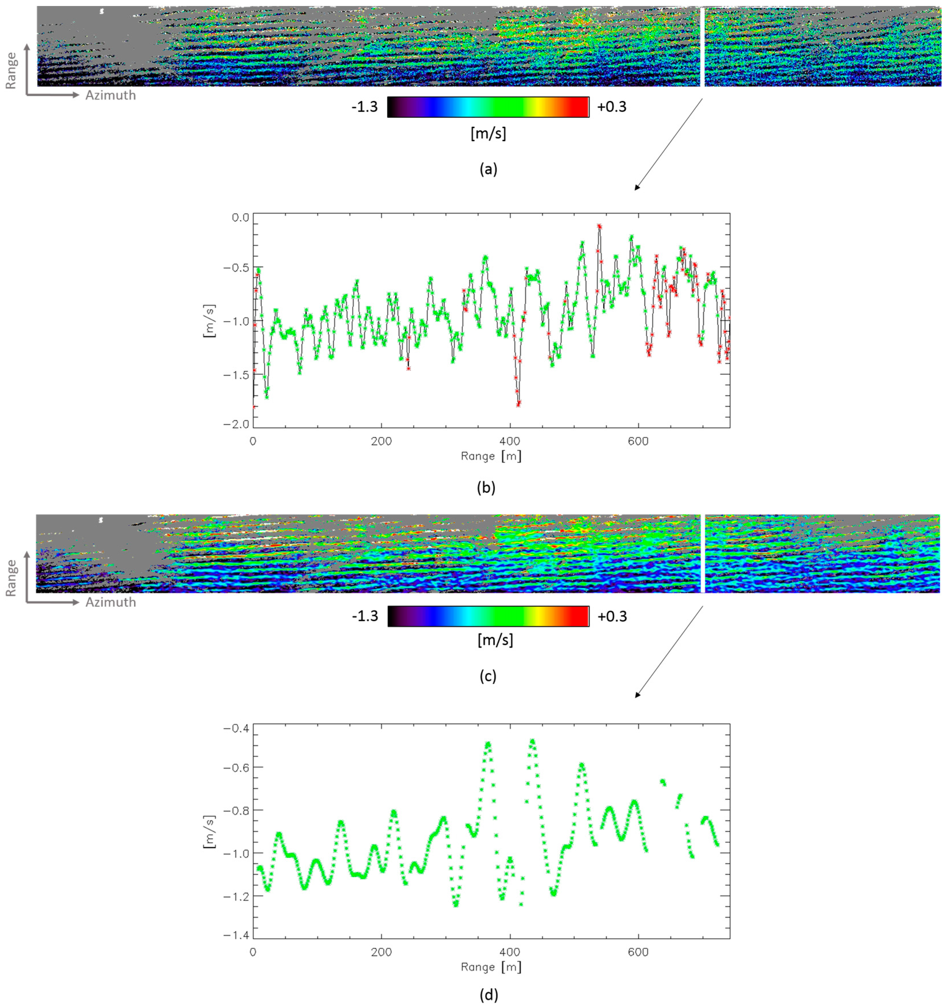
Turning to the estimated velocity, in Figure 11c, we can observe that the mean value of the estimated sea surface velocity magnitude decreases in proximity of the coastline. This behavior is clearly shown in the plot of Figure 11d, which is relevant to the same range cut of Figure 10d. As above, we have reported in Figure 11b also the corresponding cut picked up from the unfiltered map, and (as usual) we have plotted with red stars the masked (low coherence) pixels and with green stars the high coherence pixels.
A physical explanation of the decreasing trend of the estimated velocity magnitude in Figure 11d is now in order.
We recall that the velocity measured with an AT-InSAR system is the sum of different LOS contributions: the orbital motion of water particles from the swell, the phase velocity of the Bragg waves and the currents.
In our case, the swell is certainly present, as testified by the shoaling waves visible in the SAR image of Figure 2. Therefore, the LOS component of the orbital velocity certainly contributes to the u ^ r and u ^ r f i l t maps and in the corresponding range cuts reported in Figure 11. In this regard, it is worth noting that the orbital velocity is expected to increase as the waves get closer to shore. Turning to the Bragg waves, their presence cannot be excluded in our case. In this regard, it is noted that within the considered ROI the incidence angle ranges approximately from 30 to 40°; accordingly, our X-Band radar is sensitive to resonant Bragg wavelengths varying from 3.1 cm (in near range) to 2.5 cm (in far range). This means that the phase velocity of the Bragg waves detectable by our radar changes from about 27 cm/s (in near range) to 25 cm/s (in far range) [29]. Accordingly, even assuming the presence of Bragg waves, they are in any case expected to provide a very marginal contribution to the decreasing trend observed in Figure 11d for the overall measured sea surface velocity magnitude. Summing up, in our case as the sea waves move toward the shore the orbital velocity of water particles is expected to increase, whereas the phase velocity of the Bragg waves detectable by our radar is expected to be practically constant. Accordingly, we can draw the conclusion that the decreasing trend in Figure 11d is due to the presence of a sea surface current field. In this regard, it is worth noting that near the coast the currents may be generated by tides or by the river outlets (such as the Volturno one), and may become appreciable (more than 1 m/s, say) [30]: they are thus compatible with the velocity values retrieved with the proposed method.
A final consideration on the maps and plots reported in Figure 11 is necessary.
Since the LOS component of the measured sea surface velocity depends on the incidence angle, the range behavior of u ^ r and u ^ r f i l t is then somehow influenced by the variation of the incidence angle itself from the near to the far range of the considered ROI. Compensating such geometrical effect is however not a straightforward task. Indeed, in each point of the observed sea area, the orbital velocity, the phase velocity of the Bragg waves and the currents are generally three different vectors with three different amplitude and orientations. Compensation of the influence of the incidence angle in the sum of the LOS components of these three different vectors would require some information on their amplitude and orientation, which, in our case, we do not have. In this regard, it is underlined that some attempts to compensate for the geometrical effect of the incidence angle have been provided in the literature [11,31], but under precise conditions that, unfortunately, do not hold in our case. In particular, in [11], it is assumed the absence of Bragg waves and swell, whereas in [31] it is assumed the absence of swell and currents. Unfortunately, in our case these assumptions cannot be done since, as clarified above, it is likely that the swell, the sea surface currents and the Bragg waves all occur in the observed area.

5. Conclusions

In this work, we have investigated the sea surface monitoring capabilities of a three-antenna hybrid XT/AT InSAR configuration. To do this, we have focused on the on the X-Band airborne InSAeS4 SAR system. Moreover, we have proposed a very general methodology, which can be implemented with any system equipped with a three-antenna hybrid XT/AT InSAR configuration and allows simultaneous retrieval of the sea surface height and velocity through a simple linear inversion procedure. In addition, to improve the achieved sea surface height and velocity estimates, an effective filtering procedure tailored to the local properties of these sea parameters has been presented.
The shown results are relevant to a dataset acquired by the InSAeS4 SAR system in South Italy over the coastline stretch of the Campania region including the Volturno River outlet. Although in situ benchmark measurements provided by buoys or similar instruments and relevant to the time of the considered airborne mission are not available, the obtained results show some interesting evidence that the estimated quantities are physically sound.
More specifically, we have verified that the estimated velocity of the observed scene is approximately zero in correspondence of the land region. Although the paper is focused on marine scenarios and not land, this result is however interesting because it represents a good first order check of the effectiveness of the proposed procedure in separating the XT and AT contributions present in the interferograms generated through the considered three-antenna hybrid XT/AT InSAR system.
Moreover, in the marine area, we have observed that as one moves toward the coast, the estimated sea surface height increases approximately from few cm to about half meter. This behavior is physically sound and is due to the increasing level of the sea bottom when one moves toward the coast. To show this, we have compared the envelope of the sea surface height retrieved with our method and the sea wave amplitude obtained from an (even rough) available bathymetry profile of the observed area, by achieving a quite good agreement between measured and expected values.
To provide a better insight on the effectiveness of the presented approach in estimating the vertical profile of the illuminated sea surface, we have deliberately introduced a vertical bias of 1 m in a small portion of the external DEM exploited to flatten our interferograms. Then, we have shown that when applying the proposed approach, this vertical bias is effectively retrieved in the obtained sea surface height map.
Turning to the estimated sea surface velocity, we have observed that as one moves toward the coast its mean magnitude decreases approximately from 1.1 m/s to 0.8 m/s. Considering that in the observed marine area the orbital velocity of water particles is expected to increase as the sea waves move toward the shore, whereas the phase velocity of the detectable Bragg waves is expected to be practically constant, we can conclude that the decreasing trend of the measured sea surface velocity magnitude is likely due to the presence of current fields induced by tides or the Volturno River outlet. Indeed, from the literature we know that such kinds of currents near the coast may become appreciable (more than 1 m/s) and thus compatible with the values retrieved with the proposed method.
Summing up, the presented results show that the estimated quantities are physically sound. This, on the one side, provides a preliminary validation of the effectiveness of the overall presented methodology and, on the other one, highlights the potentialities of the three-antenna hybrid XT/AT InSAR configuration of the InSAeS4 system for sea state monitoring. Further validation of the achieved results is possible, and can be carried out by exploiting the analytical models provided through the literature [14] and/or through comparisons with in-situ measurements. This is however beyond the scope of this work and represents the matter of current study and the objective of future analysis.

Acknowledgments

This work has been supported by the Italian Department of Civil Protection. In addition, the author thank S. Guarino, F. Parisi and M.C. Rasulo of IREA-CNR for their support.

Author Contributions

The work has been prepared with the contribution of all the authors. In particular, A.N. has mainly worked on the data filtering and provided the physical interpretation of the proposed results; G.J. and C.E. have mainly worked on the data processing and analysis; G.F. and R.L. were the project managers of the whole SAR mission and designed the interferometric configuration of the InSAeS4 system; S.P. was the responsible of the mission planning and supervisor of the entire work.

Conflicts of Interest

The authors declare no conflict of interest.

Appendix A

In this Appendix, we show that the linear model in Equation (4) can be safely applied in our experiment. Starting from the acquisition geometry of our experiment, the mean sensor velocity reported in Table 3 and the u ^ r map shown in Figure 11, we have estimated the δϕ21 and δϕ31 terms in Equation (6) within the ROI highlighted in Figure 2. From this analysis, we obtained that, in our case, the extra phase term in Equation (6) can be safely neglected. To better show this, we focus on one azimuth coordinate (the central one) and three range coordinates (the near, the middle and far) of the considered ROI. For these coordinates, we have calculated the δr21 and δr31 terms in Equation (6), and then plotted in Figure A1 the corresponding extra phase terms |δϕ21| and |δϕ31| as a function the ur/Vx ratio. According to the mean sensor velocity reported in Table 3 and to the u ^ r map shown in Figure 11, we obtain that, in our experiment, the ur/Vx ratio belongs to the light blue region highlighted in both panels of Figure A1. As can be seen from the plots, within this region, the extra phase term in Equation (6) is always less than one degree: the linear model in Equation (4) can be thus safely applied in our case.
Figure A1. |δϕ21| (a); and | δϕ31| (b) terms in Equation (6) as a function of the ur/Vx ratio in the acquisition geometry of our experiment. In both panels, the three plots refer to the near, middle and far range within the ROI highlighted in Figure 2. In our experiment, the ur/Vx ratio belongs to the light blue region highlighted in both panels.
Remotesensing 09 00792 g014

Appendix B

In this Appendix, we show that, in our experiment, the baseline errors do not impair the accuracy of the inversion of the linear system in Equation (4).
In this regard, we recall that the calculation of both the orthogonal baseline ( b ) and the AT baseline (bAT) components in Equations (2) and (3) requires the knowledge of the positions of the phase center (PhC) of the radar antennas during the acquisition. To this aim, for each radar antenna the following procedures must be applied:
  • measurement in laboratory of the precise position of its PhC;
  • measurement of the lever arm, namely, the distance between the antenna PhC and the reference center of the Navigation Unit (NU), once they are mounted onboard the airplane; and
  • calculation of the PhC position during the flight through the exploitation of the flight data recorded by the NU.
Accordingly, errors in the baseline calculation are basically due to three sources: first, the inaccuracies in calculating the antennas’ PhC positions in laboratory; second, the inaccuracies of the lever arm measurement procedure; and, third, the inaccuracies of the NU mounted onboard the airplane. With particular reference to the NU errors, it is worth stressing that in a single pass InSAR system, such as the InSAeS4 one, the baseline calculation depends only on the attitude flight parameters (roll, pitch and yaw angles) and not by the positioning ones.
In our case, the antenna PhC positions were accurately measured in anechoic chamber [32], with an accuracy on the order of 0.1 mm [33]. The lever arms were measured just before the beginning of the flight mission by using the laser ray of an Electronic Distance Meter (EDM) integrated within a Total Station Theodolite (TST), which guarantees an accuracy of 0.5 mm [33]. Finally, the NU of the InSAeS4 system consists of modern embedded GNSS-IMU equipment [19]. In particular, thanks to the application of post-processing techniques aimed at merging GNSS and IMU data, we can achieve an accuracy of 0.005° for the roll and pitch angle measurement and of 0.008° for the yaw angle measurement (see [19]).
With reference to the proposed procedure, errors in the baseline calculation have a twofold effect. First, they impair the accuracy of the so called synthetic phase, say ϕsint, that is, the topographic phase contribution calculated from an available external DEM to obtain the flattened phase term ∆ϕ exploited by the system in Equation (1). Second they induce errors in the evaluation of the coefficients α and η in the system in Equation (1). These effects are addressed separately in the following.
To evaluate the error, say ε φ s i n t , in the calculation of the synthetic phase ϕsint, let us refer to Figure A2a, where the InSAR acquisition geometry is depicted in the vertical plane for a two-antenna system in the absence of pitch, roll and yaw. In particular, bXT is the across track baseline, that is, the baseline component reported in Figure 1b for the three available channel pairs of the InSAeS4 system. From [1] we obtain:
φ s i n t d 2 π λ b X T sin ( ϑ β r o l l )
where the angle β is depicted in Figure A2b. Moreover, just for the sake of simplicity, we have assumed the pitch and yaw angles equal to zero, since their impact in the evaluation of ϕsint is negligible with respect to that of the roll angle. The meaning of the remaining symbols in Equation (A1) is explained in the body of the paper: we just underline that hereafter in the appendix we will set d = 1 according to the InSAeS4 specifications. We also underline that the incidence angle ϑ in Equation (A1) is computed starting from the external DEM. From Equation (A1), we easily obtain that:
| ε φ s i n t | = 2 π λ | sin ( ϑ β r o l l ) | | ε b X T | < 2 π λ | ε b X T |
| ε φ s i n t | = 2 π λ b X T | cos ( ϑ β r o l l ) | | ε β + r o l l | < 2 π λ b X T | ε β + r o l l |
where ε b X T is the error in the measurement of bXT, whereas ε β + r o l l is the error in the evaluation of β and the roll angle. In particular, ε b X T ε l a + ε P h C depends on the accuracy of both the lever arm (through ε l a ) and the PhC (through ε P h C ) measurement procedures, whereas ε β + r o l l ε β + ε r o l l depends on both the accuracy of the lever arm measurement procedure (through ε β ) and the accuracy of the NU (through ε r o l l ). In our specific case, as clarified above, ε b X T is on the order of 0.6 mm. Moreover, we can safely assume that ε β < < ε r o l l , thus leading to ε β + r o l l ε r o l l , which in our case is on the order of 0.005°. From Equations (A2) and (A3), considering the InSAR configuration of the InSAeS4 system depicted in Figure 1 and the acquisition parameters reported in Table 3, we obtain that, in all the cases (that is, for both the considered channel pairs, and within the overall considered ROI), | ε φ s i n t | turns out to be less than 6.8°. Accordingly, we can safely conclude that in our case baseline errors induce negligible errors in the calculation of the flattened phase ∆ϕ in Equation (1).
Turning to the error, say ε Δ z , in the evaluation of the sea surface height ∆z in Equation (1), let us still refer to Figure A2b and assume ur = 0 in Equation (1); from Equations (1) and (2), we easily obtain:
| ε Δ z | = λ 2 π | Δ φ   r sin ϑ cos ( ϑ β r o l l ) ( b X T ) 2 | | ε b X T |
| ε Δ z | = λ 2 π | Δ φ   r sin ϑ b X T sin ( ϑ β r o l l ) cos 2 ( ϑ β r o l l )   | | ε β + r o l l |
where the meaning of all symbols in Equation (A5) is explained in the body of the paper, and use of the following relation [1]
b = b X T cos ( ϑ β r o l l )
has been done. Moreover, just for the sake of simplicity, we have again assumed the pitch and yaw angles equal to zero, since their impact in the evaluation of ∆z is negligible with respect to that of the roll angle. From Equations (A4) and (A5), from the InSAeS4 specifications discussed above and from the attitude data recorded by the NU during the flight, we obtain that, in all the cases (that is, for both the considered channel pairs, and within the overall considered ROI), | ε Δ z | turns out to be less than 3 cm, which is largely acceptable.
Turning to the error, say ε u r , in the evaluation of the sea surface velocity ur in Equation (1), let us refer to Figure A2a, where the InSAR acquisition geometry is depicted in the horizontal plane for a two antenna system in the absence of pitch, roll and yaw. In particular, bAT is the along track baseline, that is, the baseline component reported in Figure 1a for the three available channel pairs of the InSAeS4 system. Let us assume ∆z = 0 in Equation (1); from Equations (1) and (3) we easily obtain:
| ε u r | = λ 2 π | Δ φ cos ( γ + y a w ) V x   ( b A T ) 2 | | ε b A T |
| ε u r | = λ 2 π | Δ φ tan ( γ + y a w ) V x   b A T   | | ε γ + y a w |
where the angle γ is depicted in Figure A2a, whereas the meaning of all symbols in Equations (A7) and (A8) is explained in the body of the paper. Moreover, ε b A T is the error in the measurement of bAT, whereas ε γ + y a w is the error in the evaluation of γ and the yaw angle. In this case, for the sake of simplicity, we have assumed the pitch and roll angles equal to zero. Indeed, the shown results can be straightforwardly extended to the case of pitch and roll angles equal to zero.
Following the same considerations carried out above, we can say that ε b A T ε l a + ε P h C , whereas ε γ + y a w ε γ + ε y a w depends on both the accuracy of the lever arm measurement procedure (through ε γ ) and the accuracy of the NU (through ε y a w ). In our specific case, as clarified above, ε b A T is on the order of 0.6 mm. Moreover, we can safely assume that, ε γ + y a w ε y a w which in our case is on the order of 0.008°.
From Equations (A7) and (A8), from the InSAeS4 specifications discussed above and from the attitude data recorded by the NU during the flight, we obtain that in all the cases | ε u r | turns out to be less than 1.2 cm/s, and thus, once again, negligible.
Figure A2. (a) AT InSAR acquisition geometry in the horizontal plane; and (b) XT InSAR acquisition geometry in the vertical plane.
Remotesensing 09 00792 g015

Appendix C

The filter exploited in Section 4 is a bivariate raised cosine whose support is an ellipse centered around ( k ˜ x , k ˜ r ) and oriented along ψ ˜ , where the triple ( k ˜ x , k ˜ r , ψ ˜ ) is equal to ( k x u r , k r u r , ψ u r ) when the filter is tailored to u ^ r , and to ( k x Δ z , k r Δ z , ψ Δ z ) when the filter is tailored to Δ z ^ . Accordingly, the expression of the filter is the following:
H ( k x , k r ) = { 1 i f   F 1 ρ 1 2 + 1 2 cos ( π 2 ρ [ F ( k x , k r ) 1 + ρ ] ) i f 1 ρ < F 1 + ρ 0 i f F > 1 + ρ
where kx and kr are the Fourier mates of x and r, respectively; ρ is the roll-off factor; and the function F(kx,kr) sets the spectral support of the filter; its expression is:
F 2 ( k x , k r ) = ( k x k ˜ x ) 2 ( A + B cos 2 ψ ˜ 2 C ) + ( k r k ˜ r ) 2 ( A B cos 2 ψ ˜ 2 C ) ( k r k ˜ r ) ( k x k ˜ x ) B C sin 2 ψ ˜
being
A = B W / / 2 + B W 2 4 ; B = B W / / 2 B W 2 4 ; C = B W / / 2 B W 2 4
where B W / / and B W represent the filter-6 dB bandwidths along and across the direction ψ ˜ , respectively. Accordingly, in the plane kxkr, the function in Equation (A10) defines, through the equation F 2 ( k x , k r ) = 1 , an ellipse with center ( k ˜ x , k ˜ r ) , orientation ψ ˜ and axes B W / / and B W .
In the experiments presented in Section 4 the bandwidths B W / / and B W have been set through empirical inspection of the spectral content of the signal to be filtered. In particular, we have set B W / / = 0.38 rad/m and B W = 0.38 rad/m to filter u ^ r , and B W / / = 0.16 rad/m and B W = 0.6 rad/m to filter Δ z ^ . Finally, the value of the roll-off factor has been set to ρ = 0.5.

References

  1. Franceschetti, G.; Lanari, R. Synthetic Aperture Radar Processing; CRC Press: New York, NY, USA, 1999. [Google Scholar]
  2. Moreira, A.; Prats-Iraola, P.; Younis, M.; Krieger, G.; Hajnsek, I.; Papathanassiou, K.P. A tutorial on synthetic aperture radar. IEEE Geosci. Remote Sens. Mag. 2013, 1, 6–43. [Google Scholar] [CrossRef] [Green Version]
  3. Fornaro, G.; Tebaldini, S.; Perna, S.; Mariotti d’Alessandro, M.; Berardino, P.; Lanari, R.; Manzo, M.; Rocca, F.; Soldovieri, F.; Alberti, G.; et al. Interferometric experiments with the first Italian airborne P-band radar. In Proceedings of the IEEE International Geoscience and Remote Sensing Symppsium, Beijing, China, 10–15 July 2016. [Google Scholar]
  4. Aguasca, A.; Acevo-Herrera, R.; Broquetas, A.; Mallorqui, J.J.; Fabregas, X. ARBRES: Light-weight CW/FM SAR sensors for small UAVs. Sensors 2013, 13, 3204–3216. [Google Scholar] [CrossRef] [PubMed] [Green Version]
  5. Moranduzzo, T.; Melgani, F. Car speed estimation method for UAV images. In Proceedings of the IEEE International Geoscience and Remote Sensing Symppsium, Quebec City, QC, Canada, 13–18 July 2014. [Google Scholar]
  6. Monserrat, O.; Crosetto, M.; Luzi, G. A review of ground-based SAR interferometry for deformation measurement. ISPRS J. Photogramm. Remote Sens. 2014, 93, 40–48. [Google Scholar] [CrossRef]
  7. Caduff, R.; Schlunegger, F.; Kos, A.; Wiesmann, A. A review of terrestrial radar interferometry for measuring surface change in the geosciences. Earth Surf. Process. Landf. 2015, 40, 208–228. [Google Scholar] [CrossRef]
  8. Burgmann, R.; Rosen, P.A.; Fielding, E.J. Synthetic aperture radar interferometry to measure Earth’s surface topography and its deformation. Annu. Rev. Earth Planet. Sci. 2000, 28, 169–209. [Google Scholar] [CrossRef]
  9. Massonnet, D.; Feigl, K.L. Radar interferometry and its application to changes in the Earth’s surface. Rev. Geophys. 1998, 36, 441–500. [Google Scholar] [CrossRef]
  10. Bamler, R.; Hartl, P. Synthetic Aperture Radar Interferometry; Inverse Problems; IOP Publishing: Bristowl, UK, 1998; pp. R1–R54. [Google Scholar]
  11. Goldstein, R.M.; Zebker, H.A. Interferometric radar measurement of ocean surface currents. Nature 1987, 328, 707–709. [Google Scholar] [CrossRef]
  12. Goldstein, R.M.; Zebker, H.A.; Barnett, T.P. Remote sensing of ocean currents. Science 1989, 246, 1282–1285. [Google Scholar] [CrossRef] [PubMed]
  13. Romeiser, R.; Thompson, D.R. Numerical study on the along-track interferometric radar imaging mechanism of oceanic surface currents. IEEE Trans. Geosci. Remote Sens. 2000, 38, 446–458. [Google Scholar] [CrossRef]
  14. Romeiser, R.; Breit, H.; Eineder, M.; Runge, H.; Flament, P.; de Jong, K.; Vogelzang, J. Current measurements by SAR along-track interferometry from a Space Shuttle. IEEE Trans. Geosci. Remote Sens. 2005, 43, 2315–2324. [Google Scholar] [CrossRef]
  15. Romeiser, R.; Runge, H. Theoretical evaluation of several possible along-track InSAR modes of TerraSAR-X for ocean current measurements. IEEE Trans. Geosci. Remote Sens. 2007, 45, 21–35. [Google Scholar] [CrossRef]
  16. Bao, M.; Alpers, W.; Bruning, C. A new nonlinear integral transform relating ocean wave spectra to phase image spectra of an along-track interferometric synthetic aperture radar. IEEE Trans. Geosci. Remote Sens. 1999, 37, 461–466. [Google Scholar] [CrossRef]
  17. Suchandt, S.; Runge, H.; Breit, H.; Steinbrecher, U.; Kotenkov, A.; Balss, U. Automatic extraction of traffic flows using TerraSAR-X along-track interferometry. IEEE Trans. Geosci. Remote Sens. 2010, 48, 807–819. [Google Scholar] [CrossRef]
  18. Siegmund, R.; Bao, M.; Lehner, S.; Mayerle, R. First demonstration of surface currents imaged by hybrid along- and cross-track interferometric SAR. IEEE Trans. Geosci. Remote Sens. 2004, 42, 511–519. [Google Scholar] [CrossRef]
  19. Perna, S.; Esposito, C.; Amaral, T.; Berardino, P.; Jackson, G.; Moreira, J.; Pauciullo, A.; Vaz Junior, E.; Wimmer, C.; Lanari, R. The InSAeS4 airborne X-band interferometric SAR system: A first assessment on its imaging and topographic mapping capabilities. Remote Sens. 2016, 8, 40. [Google Scholar] [CrossRef]
  20. Perna, S.; Berardino, P.; Britti, F.; Cirillo, C.; Esposito, C.; Fornaro, G.; Lubeck, D.; Monaldi, G.; Moreira, J.; Pauciullo, A.; et al. Capabilities of the TELAER airborne SAR system upgraded to the multiantenna mode. In Proceedings of the IEEE International Geoscience and Remote Sensing Symppsium, Munich, Germany, 22–27 July 2012; pp. 1545–1548. [Google Scholar]
  21. Moreira, A.; Huang, Y. Airborne SAR processing of highly squinted data using a chirp scaling approach with integrated motion compensation. IEEE Trans. Geosci. Remote Sens. 1994, 32, 1029–1040. [Google Scholar] [CrossRef]
  22. Rabus, B.; Eineder, M.; Roth, A.; Bamler, R. The shuttle radar topography mission—A new class of digital elevation models acquired by spaceborne radar. ISPRS J. Photogramm. Remote Sens. 2003, 57, 241–262. [Google Scholar] [CrossRef]
  23. Perna, S.; Esposito, C.; Berardino, P.; Pauciullo, A.; Wimmer, C.; Lanari, R. Phase offset calculation for airborne InSAR DEM generation without corner reflectors. IEEE Trans. Geosci. Remote Sens. 2015, 53, 2713–2726. [Google Scholar] [CrossRef]
  24. Raney, R.K. Synthetic aperture imaging radar and moving targets. IEEE Trans. Aerosp. Electron. Syst. 1971, 3, 499–505. [Google Scholar] [CrossRef]
  25. Krieger, G.; Moreira, A.; Fiedler, H.; Hajnsek, I.; Werner, M.; Younis, M.; Zink, M. TanDEM-X: A satellite formation for high-resolution SAR interferometry. IEEE Trans. Geosci. Remote Sens. 2007, 45, 3317–3334. [Google Scholar] [CrossRef] [Green Version]
  26. Esposito, C.; Pauciullo, A.; Berardino, P.; Lanari, R.; Perna, S. A simple solution for the phase offset estimation of airborne SAR interferograms without using corner reflectors. IEEE Geosci. Remote Sens. Lett. 2017, 14, 379–383. [Google Scholar] [CrossRef]
  27. Navionics. Available online: https://www.navionics.com (accessed on 1 April 2017).
  28. Salmon, R. Lectures on the Course Introduction to Ocean Waves. Available online: http://pordlabs.ucsd.edu/rsalmon/111.textbook.pdf (accessed on 1 April 2017).
  29. Martin, S. An Introduction to Ocean Remote Sensing; Cambridge University Press: Cambridge, UK, 2004; Chapter 2. [Google Scholar]
  30. Holthuijsen, L. Waves in Shallow Water, in Guide to Wave Analysis and Forecasting, 2nd ed.; Sectretariat of the World Meteorological Organization: Geneva, Switzerland, 1998. [Google Scholar]
  31. Marom, M.; Shemer, L.; Thornton, E.B. Energy density directional spectra of a nearshore wave field measured by interferometric synthetic aperture radar. J. Geophys. Res. 1991, 96, 22125–22134. [Google Scholar] [CrossRef]
  32. Perna, S.; Esposito, C.; Pauciullo, A.; Romano, P.; Gifuni, A. A fast approach for antenna phase center evaluation. In Proceedings of the IEEE International Geoscience and Remote Sensing Symppsium, Quebec City, QC, Canada, 13–18 July 2014. [Google Scholar]
  33. Wimmer, C.; Siegmund, R.; Schwabisch, M.; Moreira, J. Generation of high precision DEMs of the Wadden Sea with airborne interferometric SAR. IEEE Trans. Geosci. Remote Sens. 2000, 38, 2234–2245. [Google Scholar] [CrossRef]
Figure 1. The interferometric layout of the InSAeS4 system. The Three antennas are denoted as A1, A2, and A3. (a) Horizontal plane: The z-axis points downward. (b) Vertical plane: The x-axis points ahead.
Remotesensing 09 00792 g001
Figure 2. Multi-look amplitude SAR image relevant to the acquired data. Spatial resolution: 6 m × 5 m (slant range × azimuth). The white frame highlights the region of interest considered for the filtering procedure summarized in Figure 9.
Remotesensing 09 00792 g002
Figure 3. (a) AT baseline components for ∆ϕ21 and ∆ϕ31 interferograms as a function of the azimuth coordinates; and (b) the orthogonal baseline components for ∆ϕ21 and ∆ϕ31 interferograms as a function of the range coordinates.
Remotesensing 09 00792 g003
Figure 4. The unwrapped and flattened interferograms: ∆ϕ21 (a); and ∆ϕ31 (b). (c) We have superimposed (in gray) the mask obtained by selecting the pixels whose coherence is smaller than 0.7 at least in one of the two interferograms. Spatial resolution: 6 m × 5 m (slant range × azimuth).
Remotesensing 09 00792 g004
Figure 5. The estimated surface height Δ z ^ . We have superimposed (in gray) the mask of Figure 4c. Spatial resolution: 6 m × 5 m (slant range × azimuth).
Remotesensing 09 00792 g005
Figure 6. The estimated surface velocity map u ^ r . We have superimposed (in gray) the mask of Figure 4c. Spatial resolution: 6 m × 5 m (slant range × azimuth).
Remotesensing 09 00792 g006
Figure 7. The vertical height (in radar grid) of the external DEM exploited to flatten the InSAeS4 interferograms. The vertical height reported in the figure has been obtained starting from the SRTM vertical height and applying a 1 m bias in the triangular area in the bottom-left corner.
Remotesensing 09 00792 g007
Figure 8. The same as Figure 6, but after exploiting the external DEM of Figure 7 (rather than the original SRTM one) to flatten the available interferograms. We have superimposed (in gray) the mask of Figure 4c.
Remotesensing 09 00792 g008
Figure 9. Block diagram of the filtering procedure applied to the estimated sea surface velocity and height maps. In the former case, the symbol g stands for ur; in the latter one for ∆z.
Remotesensing 09 00792 g009
Figure 10. Sea surface height map: before (a); and after (c) the filtering procedure, with the mask of Figure 4c superimposed (in gray). The range cut is highlighted in white (a,c); and is plotted in (b,d).
Remotesensing 09 00792 g010
Figure 11. Sea surface velocity map: before (a); and after (b) the filtering procedure, with the mask of Figure 4c superimposed (in gray). The range cut is highlighted in white (a,c); and is plotted (b,d).
Remotesensing 09 00792 g011
Figure 12. Envelope of the estimated sea surface height profile of Figure 10d (green stars) with superimposed the expected trend of the theoretical sea wave amplitude obtained from the external bathymetry using the expression in Equation (9) (black solid line).
Remotesensing 09 00792 g012
Figure 13. Envelope of the filtered sea surface height map of Figure 10c: before (a); and after (b) the normalization to the theoretical sea wave amplitude obtained from the external bathymetry using the expression in Equation (9). We have superimposed (in gray) the mask of Figure 4c.
Remotesensing 09 00792 g013
Table 1. Main airplane features.
Feature
ModelLearJet 35A
Propulsion2 Turbofan Garret T731
Velocityup to 800 km/h
Autonomy4000 km
Altitudeup to 8.40 km
Table 2. Main radar parameters.
Parameter
Carrier Frequency9.55 GHz
Carrier wavelength0.0314 m
Bandwidth50–400 MHz
PRF0.20–16 kHz
Number of antennas3
PolarizationHH
Table 3. Main mission and processing parameters.
Parameter
Bandwidth100 MHz
Range pixel spacing (*)1.50 m
Azimuth pixel spacing (*)0.15 m
Mean aircraft altitude5.2 km
Mean aircraft velocity127 m/s
Geometric resolution (range × azimuth)1.50 m × 0.50 m
Range swath 3 km
Look angle29–55°
(*) Focused data.

