A Robust Inversion Algorithm for Surface Leaf and Soil Temperatures Using the Vegetation Clumping Index
by
 ,
,
Zunjian Bian
1,2 ,
,
Biao Cao
1,†,
Hua Li
1,†,
Yongming Du
1,*,
Lisheng Song
3,
Wenjie Fan
4,
Qing Xiao
1,† and
Qinhuo Liu
1,*
1
State Key Laboratory of Remote Sensing, Institute of Remote Sensing and Digital Earth, Chinese Academy of Sciences, Beijing 10010, China
2
College of Resources and Environment, University of Chinese Academy of Sciences, Beijing 100049, China
3
Chongqing Key Laboratory of Karst Environment School of Geographical Sciences, Southwest University, Chongqing 400712, China
4
Institute of RS and GIS, Peking University, Beijing 100871, China
*
Authors to whom correspondence should be addressed.
†
These authors contributed equally to this work.
Remote Sens. 2017, 9(8), 780; https://doi.org/10.3390/rs9080780
Submission received: 12 June 2017
/
Revised: 13 July 2017
/
Accepted: 28 July 2017
/
Published: 30 July 2017
(This article belongs to the Special Issue Remote Sensing for Land Surface Temperature (LST) Estimation, Generation, and Analysis)
Abstract
:The inversion of land surface component temperatures is an essential source of information for mapping heat fluxes and the angular normalization of thermal infrared (TIR) observations. Leaf and soil temperatures can be retrieved using multiple-view-angle TIR observations. In a satellite-scale pixel, the clumping effect of vegetation is usually present, but it is not completely considered during the inversion process. Therefore, we introduced a simple inversion procedure that uses gap frequency with a clumping index (GCI) for leaf and soil temperatures over both crop and forest canopies. Simulated datasets corresponding to turbid vegetation, regularly planted crops and randomly distributed forest were generated using a radiosity model and were used to test the proposed inversion algorithm. The results indicated that the GCI algorithm performed well for both crop and forest canopies, with root mean squared errors of less than 1.0 °C against simulated values. The proposed inversion algorithm was also validated using measured datasets over orchard, maize and wheat canopies. Similar results were achieved, demonstrating that using the clumping index can improve inversion results. In all evaluations, we recommend using the GCI algorithm as a foundation for future satellite-based applications due to its straightforward form and robust performance for both crop and forest canopies using the vegetation clumping index.

1. Introduction
Land surface temperature (LST) is an important forcing variable for physical processes in surface–atmosphere interactions, including the energy budget and the hydrological cycle [1,2]. In the context of remote sensing applications, LST inversion can currently be performed at multiple spatial and temporal scales [3,4,5,6], and the accuracy of the satellite-based LST product is close to or less than 1.0 K [7,8]. The importance of the temperature distribution in heterogeneous and non-isothermal pixels has been increasingly recognized for the full characterization of the surface temperature state.
This issue arises from surface temperature differences between components of a vegetation–soil system during most of the day because of the inhomogeneity of the intrinsic structures and physical properties. These differences can reach up to 11.0 °C, as has been reported in many in situ experiments [9,10,11]. This temperature information can facilitate understanding the complicated physical processes in energy and radiative transfers. For instance, these temperature differences are a factor that leads to the directional anisotropy of measured radiance in the thermal infrared (TIR) domain. This anisotropy makes directly comparing LSTs retrieved from a study area using different images difficult due to the viewing angle dependence [6]. To improve the quality of LST to fit a reference viewing angle, information about the surface temperature difference should be considered. Moreover, a practical two-source energy balance (TSEB) model developed by Norman et al. [12] and Kustas et al. [13,14] has been applied for various landscapes, with consideration of the temperature difference between the leaves and soil. Accurate surface component temperatures are, therefore, primarily required to derive evapotranspiration [15]. However, no component temperature product has yet been released despite the wide potential use.
Multi-angle remote sensing has been identified as a useful tool for the separation of leaf and soil temperatures [16,17]. Previous efforts have been directed toward inverting component temperatures using both experimental and satellite-borne multi-angle datasets [16,17,18,19]. Many directional algorithms have been proposed based on radiative transfer models (RTMs), such as the geometric model proposed by Kimes et al. [20] for row-planted crops and the analytical RTM known as FR97 proposed by Francois et al. [21] for homogenous canopies. Using these RTMs, the temperatures of surface sunlit and shaded areas and their vertical distributions can be inverted. For instance, Timmermans et al. [16] retrieved four-component (sunlit and shaded leaves and sunlit and shaded soil) temperatures using the four-stream scattering by arbitrarily inclined leaves (4SAIL) model. Colaizzi et al. [22] proposed a radiometer footprint model to estimate sunlit and shaded components for row crops. However, because most of these algorithms were limited to a specific scene, they are not robust enough for the several possible landscapes in a satellite pixel.
Li et al. [19] and Jia et al. [18] proposed a practical inversion algorithm that uses the normalized difference vegetation index (NDVI) to invert leaf and soil temperatures from a satellite pixel. Shi et al. [23] proposed a combined model with consideration of the bare soil in a satellite pixel. However, acquiring the rate of bare soil in a satellite pixel is not easy, particularly in the mixed pixels of sparse forest and bare soil. To some extent, the effects of different types of pixels on component temperature inversion are due to the vegetation clumping phenomena related to the study objects, i.e., mostly crop and forest plants. This vegetation clumping effect can be quantitatively described using the clumping index, which is a vital structural parameter used to accurately estimate the gap frequency in various landscapes, especially sparse forest [24]. Therefore, using the clumping index of leaves represents a good option for determining the vegetation distribution pattern in a satellite pixel. Thus, applying the clumping index to component temperature inversion appears to be acceptable and practical. Anderson et al. have analyzed the effects of vegetation clumping on estimating evapotranspiration [25], but its effects on component temperature inversion have not been completely analyzed.
In this paper, we propose an inversion procedure for leaf and soil surface temperatures using the gap frequency with clumping index (hereafter referred to as GCI). This algorithm was evaluated against both simulated and measured surface temperatures over several small-scale scenes. We selected a novel radiosity model, i.e., radiosity applicable to porous individual objects (RAPID) proposed by Huang et al. [26], as the benchmark for forward simulations. The measured dataset was collected by the wide-angle infrared dual mode line/area array scanner (WIDAS) sensor over orchard, maize and wheat canopies. In this paper, the evaluations mostly depend on simulated datasets because of the scarcity of experimental datasets that provide surface directional observations and synchronous component temperatures. Although a temperature difference between sunlit and shaded portions exists, only two components of the leaf and soil were assumed in the paper. In Section 2, the GCI inversion algorithm is introduced. Then, this proposed inversion algorithm is evaluated using simulated and measured datasets in Section 3 and Section 4, respectively. Section 5 provides a short summary of the paper.
2. Inversion Algorithm
2.1. Inversion Method
Thermal radiance, as observed by an infrared sensor aboard an aircraft or satellite, is usually treated as a linear combination of the radiance from the land surface and the upward radiance from the atmosphere, as shown in Equation (1). The radiance from the land surface can also be divided into an emission term due to surface components (leaves and soil) and a ground-reflected term due to the downward radiance from the atmosphere, as shown in Equation (2). In these two equations, each component is assumed to have a homogeneous temperature.
where and represent the viewing zenith angle (VZA) and viewing azimuth angle (VAA), respectively; is the radiance observed at ground level; is the effective transmittance of the atmosphere; and are the upward and downward atmospheric radiances, respectively; is the Planck radiative function; and are the component temperature and component effective emissivity (CEE), respectively; represents the surface total effective emissivity; and the subscripts and s represent the leaves and soil, respectively.
In this paper, the CEE is defined differently from the material emissivity because multiple scattering radiation and the visible proportions of the components are both considered according to the conceptual model of Chen et al. [27]. This effective emissivity is related to the viewing angle and is used to explain the directional anisotropy of measurements in the TIR domain [28]. Because the estimation error of the atmospheric effect appears equivalent in different algorithms according to Equation (2), we assume that this effect can be eliminated in the data pre-processing, despite the fact that atmospheric correction always plays an important role in LST inversion. The inversion equation can be simplified to a linear equation after atmospheric correction. In general, the temperature emissivity separation is an underdetermined problem. For the component temperature inversion, the emissivity values of the leaf and soil are known. Therefore, the inversion results are directly related to the accuracy of the CEE as reported in Equations (3) and (4).
where and represent the zenith angles of the two observations. Many optimized algorithms, such as least-square, Bayes, and genetic algorithms have been proposed to improve the inversion results [16,29,30,31]. Since only two observed angles are used and direct results can be clear, we do not use an optimization algorithm in this paper. Thus, the estimation of the CEE and the analysis of the effects on the inversion results are the core of the component temperature inversion.
2.2. Component Effective Emissivity
According to many radiative transfer theories, such as 4SAIL and FR97, the CEE is mainly composed of (1) the direct emissions of the components and (2) the multiple scattering radiation between components, as follows:
where represents the gap frequency; represents the visible proportion of leaves; and and represent the leaf and soil material emissivity values, respectively. The subscript m () represents the multiple scattering contribution to the CEE. In this algorithm, the surface gap frequency is estimated using Equation (7) according to Nilson et al. [24].
where G represents the mean projection of the unit foliage area in the viewing or solar direction, which is set to 0.5 for the spherical leaf inclination distribution function (LIDF). is the leaf area index, and is a vegetation dispersion parameter at a given zenith angle with a value ranging from 1.0 to close to 0. When is 1.0, the canopy is random. The vegetation dispersion parameter is also described by the clumping index [32]. Accurate gap frequencies can be calculated once the clumping index and the leaf area index (LAI) are accurately determined. The CEE is important to the inversion results, and it will be introduced in detail in the next sub-section. An analytical method in the FR97 model is used for the multiple scattering radiation. In the FR97 model, the multiple scattering contribution for soil is ignored, and the multiple scattering contribution for leaves can be estimated as follows (Equation (9)):
where M represents the hemispheric average gap frequency [21]; and is the cavity effect coefficient. According to Ren et al. [33], this value can be estimated using the 4SAIL model. The FR97 model provides analytical expressions for the effective emissivity of leaves and soil over a homogeneous scene. The GCI algorithm can be considered a combination between the FR97 model and the inversion algorithm of the vegetation clumping index, and the latter is described below.
2.3. Vegetation Clumping Index
According to Equations (5)–(7), the clumping index is of importance for CEE. Although the clumping index is directional, the average clumping index can be used for crop scenes, which is defined as the ratio between the effective LAI and actual LAI values. It can be owing to the fact that the 4SAIL model performed well over many crop canopies with effective LAI values [34]. Currently, several algorithms have been proposed to calculate the average vegetation clumping information [35].
As for sparse forest canopies, strong vegetation clumping effects usually exist. A practical algorithm to estimate the vegetation clumping index of savanna canopies was proposed by Li et al. [36]. In this paper, the clumping effect contributed by tree crowns was retrieved using the gap frequency as follows:
where represents the gap frequency of the forest in direction ; is the crown count density; is the horizontal crown radius; represents the interception proportion by tree crowns; represents the gaps within crowns; represents the actual LAI of a single tree; and is the viewing zenith angle in the transformed dimension, which can be calculated using and the vertical crown radius, , as in Equation (11):
In addition, the row-planted structure always plays a vital role in a temperature inversion over a small-scale study area. To accurately estimate the clumping index in this case, an algorithm proposed by Yan et al. [37] is recommended. The average gap frequency across the row direction can be described as follows (Equation (12)):
where a and c refer to the row width and row spacing, respectively; H represents the height of the canopy; and u represents the leaf volume density function.
3. Sensitivity Analysis
This section demonstrates the performance of the new inversion algorithm by comparing it to two existing algorithms using a simulated dataset. The two existing algorithms are based on the FR97 model and the NDVI. A forward dataset generated by the RAPID model was used to examine the precision of the estimated effective emissivity and to explore the performance of the inversion algorithm. The RAPID model is a novel computer graphics-based radiosity model applicable to porous individual thin objects [26]. In the GCI algorithm, the sources of error in the retrieved results were mainly from the clumping index and the LAI. Therefore, their effects are also analyzed in this section.
3.1. Simulated Dataset
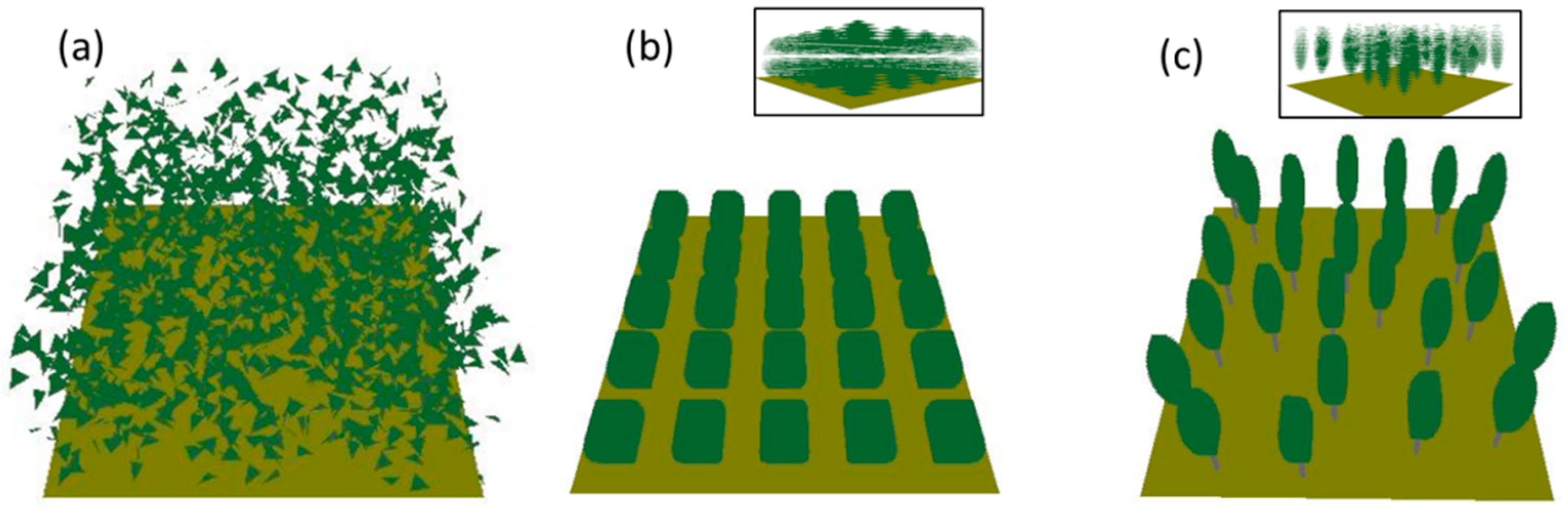
In nature, surface component temperatures result from the energy balance in a specific canopy structure under certain meteorological conditions. To assess the sensitivity of the effective emissivity and inversion scheme, we constructed three typical scenes in this study—turbid canopies, regularly planted crops and randomly distributed forest—as shown in Figure 1. Strictly speaking, a real turbid canopy does not exist in nature. However, dense canopies are usually treated as turbid, and many models have been proposed based on the assumption of a turbid canopy, such as the 4SAIL and FR97 models. In this study, turbid scenes were constructed with vegetation leaves composed of many equilateral triangular facets. The facets had a random spatial distribution, and their zenithal angle distribution followed the spherical LIDF. The crop scenes were composed of regularly arranged vegetation objects with a row and column spacing of 0.5 m. These objects were composed of many porous square facets, and their size increases as the LAI value of the scene increases. Note that although row-planted crops are common in nature, we constructed only regularly planted crop scenes in this simulated dataset because it is difficult to consider the row orientation in pixels with low spatial resolutions. The forest scenes were composed of randomly distributed ellipsoidal objects with a horizontal to vertical crown radius ratio of one to three and a single tree LAI value of 6.0. The LAI value of the forest scene was related to the density of these objects. Although RAPID can work well for both flat leaves and conifer shoots, we used only the broadleaf case in the forest scene and did not consider the effect of the trunks. Limiting the dataset to porous objects rather than real-structure canopy scenarios, such as maize and wheat, does not jeopardize the degree of representativeness because we focus on a universal case rather than a specific one in the evaluation process. All of the scenes were generated as an infinite canopy by juxtaposing identical scenes.
Three categories of input must be considered to produce the simulated dataset: the canopy geometrical structure, the component emissivity and the component temperature. In this study, we first simulate 14 scenarios for different conditions (consisting of two component emissivity profiles and seven canopy structures). Next, five temperature profiles were applied independently in these scenarios. The simulated dataset is shown in Table 1, in which represents the temperature difference between the leaves and soil and and represent the component reflectance and transmittance, respectively.
The canopy structure is a vital factor that determines the surface radiative transfer. The surface gap frequency varies with vegetation growth, and we therefore selected LAI values varying from 0.5 to 3.5 with a step size of 0.5 for different growth periods. In this simulated dataset, we did not select growth periods with LAI values greater than 3.5 because small directional variations could appear. In nature, the average soil temperature is predominantly affected by shaded soil under a dense vegetation canopy. In this case, the temperature difference between the leaves and the soil is not expected to be large. In addition, only a spherical LIDF is discussed in this paper. Based on the scene directional projection in the RAPID model, the effective LAI, , can be calculated with the gap frequency described above as follows (Equation (13)):
The component material emissivity can significantly influence the multiple scattering contribution. The emissivity values of leaf and soil material mainly range from 0.96 to 0.99 and from 0.90 to 0.98, respectively. In this simulated dataset, two emissivity profiles were used: a high-emissivity profile (0.99 and 0.97 for leaves and soil, respectively) and a low-emissivity profile (0.97 and 0.93 for leaves and soil, respectively).
The temperature profile can be simulated using the temperature difference between the leaves and soil. In this paper, we simulated five temperature profiles with differences of 0 °C, 5.0 °C, 10.0 °C, 15.0 °C and 20.0 °C, and a leaf temperature of 25 °C.
To examine the precision of the CEE, we compared simulations with VZAs varying from 0 to 60° with a step size of 5°. In the inversion process, only two VZAs (nadir and a forward inclination of 55°) were used. Because the NDVI was used in the NDVI algorithm, we also simulated the surface directional reflectance in the red (670 nm) and near-infrared (NIR) (870 nm) bands.
3.2. Inversion by the FR97 and NDVI Algorithms
Equations (5)–(9) can be used for the FR97 algorithm. However, the vegetation clumping effect was not considered. Therefore, the vegetation clumping index was set to 1.0 in the inversion process. For the NDVI algorithm, the CEE was also determined using Equations (5) and (6), but the gap frequency was estimated via the following empirical method using the NDVI [18]:
where and are the NDVI values corresponding to an infinite leaf area and to bare soil, respectively; and is the fitting coefficient. In this simulated dataset, the coefficient k was determined by fitting the actual gap frequency of the scene with values of 0.65, 0.53 and 0.64 for turbid, crop and forest scenes, respectively. For the FR97 and GCI algorithms, the LAI value is required for the gap frequency by using an exponential expression. For practical applications, the NDVI value is directly determined by an empirical method, and the multiple scattering effect is also simplified by using slightly higher material emissivity values of 0.99 and 0.97 for leaves and soil, respectively [18].
3.3. Results
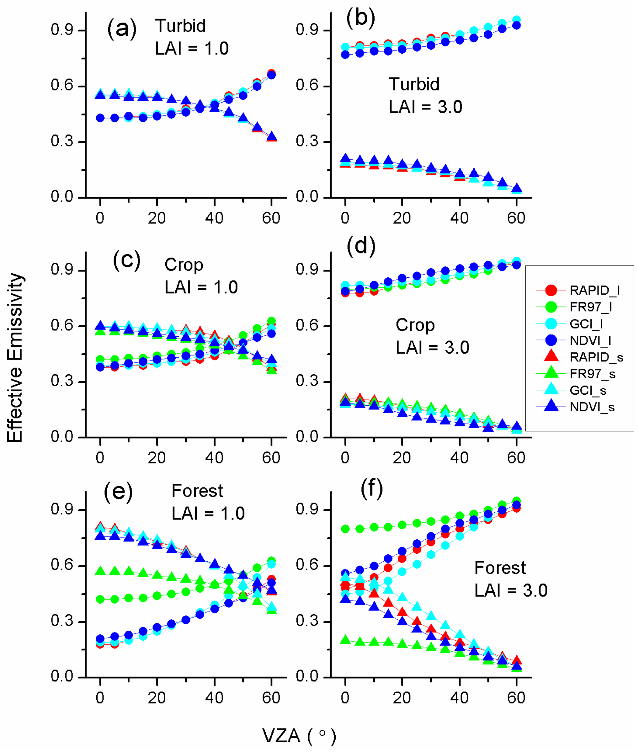
Figure 2 depicts comparisons of the simulated and reference CEE values for three scenes with LAI values of 1.0 and 3.0. Similar angular variations in the CEE with the VZAs were estimated, and an increase in VZA leads to an increase in the effective emissivity of leaves and a decrease in the effective emissivity of soils. In this paper, the directional variation was defined as the difference between the off-nadir and nadir values. For the turbid canopies, we assumed that the leaf dispersion was completely random with an average clumping index of 1.0. Therefore, the same performance can be found by using the FR97 and GCI algorithms. Regarding the NDVI algorithm, a good agreement can be found for the scene with an LAI value of 1.0, but a slight underestimation of the leaf effective emissivity and a slight overestimation of the soil effective emissivity appeared over the scene with an LAI value of 3.0. Similar performances are found for both crop and turbid scenes. However, regarding the FR97 algorithm, a slight overestimation of leaf effective emissivity and a slight underestimation of the soil effective emissivity appeared. Nevertheless, the shape of the simulated angular variations was still similar to the reference. Regarding the NDVI algorithm, the shape of simulated angular variations was slightly different from the reference, particularly at VZAs ranging from 20 to 40°. For forest scenes, stronger angular variations of CEE were found compared with those over turbid and crop scenes. The FR97 algorithm resulted in clear overestimations of the leaf effective emissivity and underestimations of the soil effective emissivity relative to the reference. Additionally, the maximum difference appeared at nadir. Slight overestimations and slight underestimations were found for the angular variations simulated by the GCI and NDVI algorithms, respectively.
Figure 3 shows the difference distribution between the retrieved and reference component temperatures. Their root mean squared errors (RMSEs) can be found in Figure 4. Over turbid and crop scenes, the FR97 and GCI algorithms performed similarly, with RMSEs less than 1.0 °C. Over crop scenes, because the average clumping index was used in the GCI algorithm, the RMSEs of the retrieved results were slightly lower than those of the FR97 algorithm. Regarding the NDVI algorithm, the retrieved results over crop scenes were less satisfactory, with an obvious overestimation of the soil temperatures. Over forest scenes, the best results were retrieved using the GCI algorithm, and the performance of the NDVI algorithm was acceptable, with RMSEs of approximately 2.0 °C. However, the soil temperatures obtained with the FR97 algorithm were considerably overestimated, which corresponded to an obvious peak on the right side of the soil histogram in Figure 3f.
3.4. Effect of the Clumping Index Error
Regarding the FR97 algorithm, the sources of error in the gap frequency are associated with the assumption of a homogeneous canopy. According to the performance of the FR97 and GCI algorithms, because of the vegetation clumping effect over crop scenes, the RMSEs of the retrieved results using the GCI algorithm were lower than those using the FR97 algorithm. The vegetation clumping effect was stronger in forest scenes than in crop scenes, as shown in Figure 5a. In this case, the angular variation of the CEE was obviously underestimated by the FR97 algorithm. This underestimation could result in an overestimation of the temperature difference between the leaves and the soil, depending on the angular variation in the observations. According to the retrieved results over forest scenes, this discrepancy may result in soil RMSE values greater than 15.0 °C. Regarding the NDVI algorithm, no clumping information was required, and acceptable results appeared over turbid and forest scenes, whereas large discrepancies appeared over crop scenes. This difference may be because the gap frequency in a serially planted crop scene, in which the LAI increases as the plant size increases, cannot be accurately estimated by an empirical method. And the fitting coefficients determined by reference gap frequencies ranging from 0 to 60° may not always accurately mimic its angular variation between the nadir and 55°.
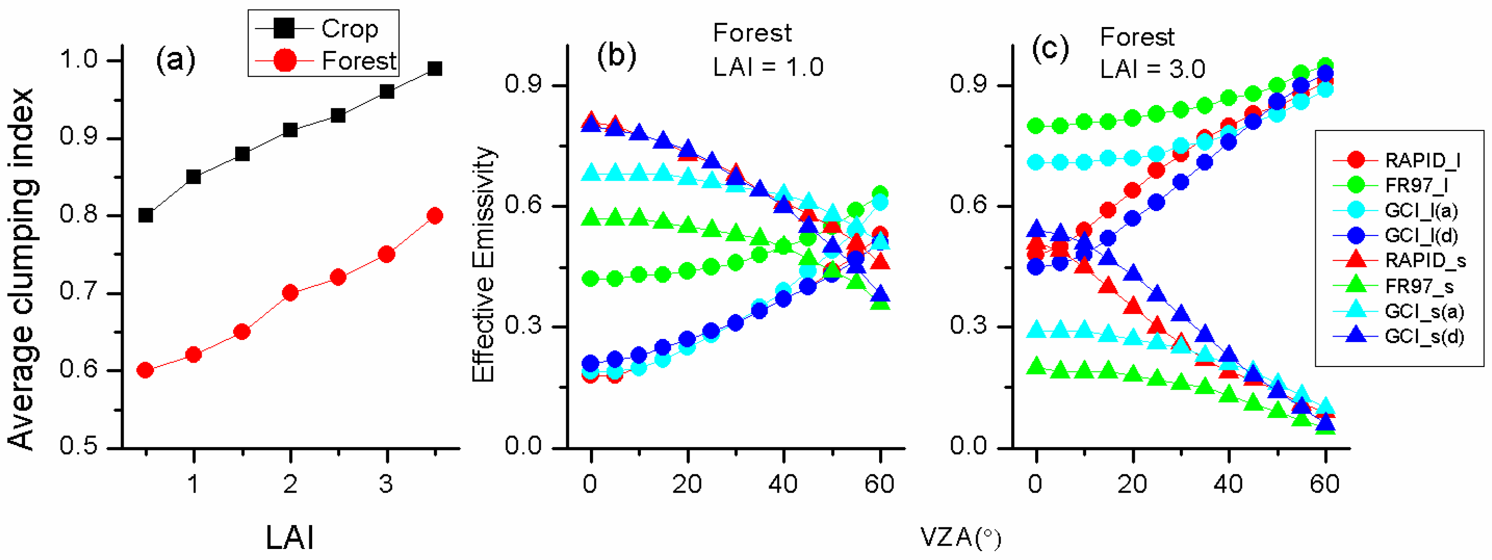
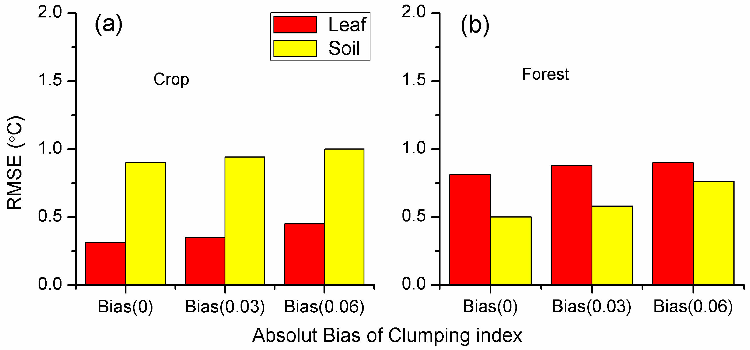
These comparisons demonstrate that the use of the clumping index improves the retrieved results. Because the average clumping index can usually be easily acquired, the question then arises as to whether the directional clumping index can be replaced over forest scenes. To discuss this question, the average clumping index was applied to forest scenes as shown in Figure 5b,c. Compared to the FR97 algorithm, the average clumping index led to considerable improvements in simulating the CEE, but the simulated CEE using the directional clumping index still agreed better with the reference. To analyze the effect of the error in the clumping index, biases of ±0.03 and ±0.06 were imposed on the inversion process. Figure 6a,b show the RMSEs over crop and forest scenes, respectively, when a bias was imposed. The results show that the clumping index bias had no significant effect on the inversion results. It is not surprising that such biases in the clumping index had a limited effect on in Equation (7).
3.5. Effect of the LAI Error
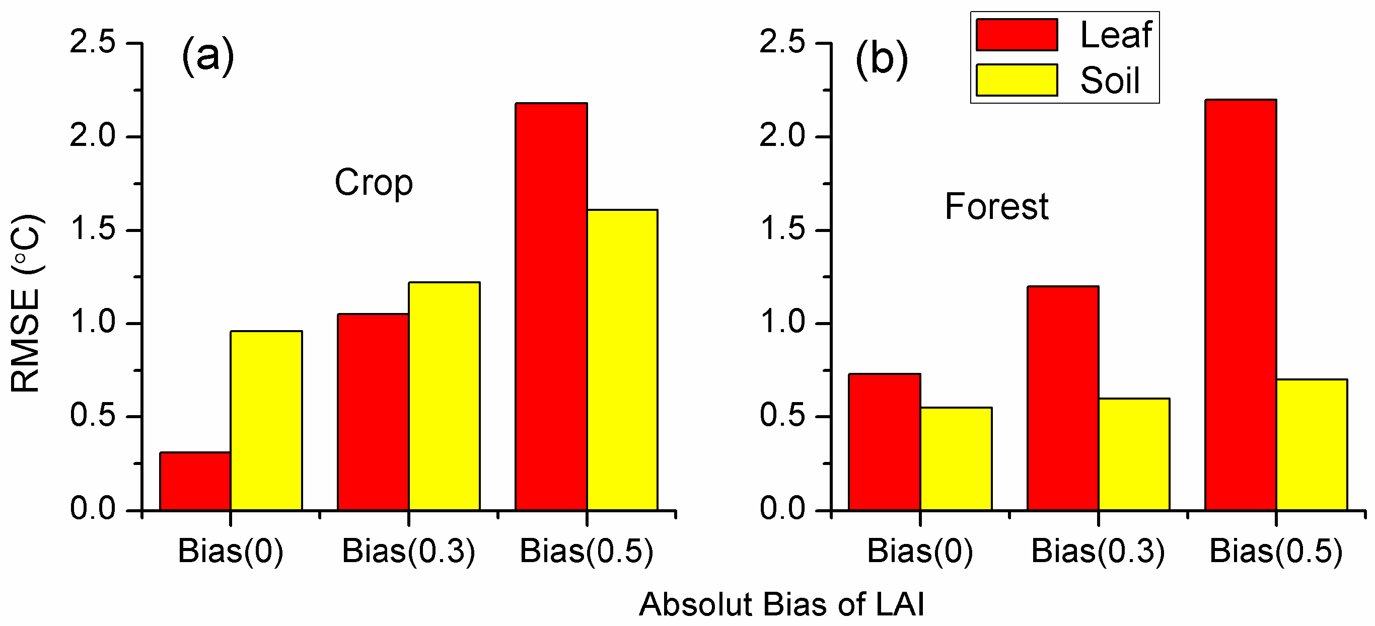
Strictly speaking, we do not consider the effect of the LAI error on the retrieved temperatures in the GCI algorithm; however, this error does not exist in the NDVI algorithm. Figure 7a,b show the RMSEs of the results retrieved by the GCI algorithm over crop and forest scenes with imposed LAI biases of ±0.3 and ±0.5. In this case, only LAI values varying from 1.0 to 3.5 were considered. When the LAI bias increased, RMSEs of both leaf and soil temperatures increased, especially for leaves. In addition, the soil RMSEs in the forest scenes are affected less by the imposed LAI biases than those in the crop scenes. It is mainly due to the fact that a stronger vegetation clumping effect occurred in the forest scenes as shown in Figure 5a, that the results show larger angular variations of the CEE. When LAI biases of ±0.3 and ±0.5 were imposed, the RMSEs of the retrieved leaf temperatures were approximately 1.0 °C and 2.0 °C, respectively. Therefore, the LAI played a vital role in the component temperature inversion.
4. Inversion Validation
4.1. Experimental Campaign
The WIDAS data were used to test the proposed inversion scheme. The observations over orchard canopies were from the Heihe Watershed Allied Telemetry Experimental Research (HiWATER) campaign [38], which took place in an arid region in Gansu Province, China. During the HiWATER campaign, multi-angle observations over orchard canopies (100.369° E, 38.845° N) were derived by an airplane platform on 3 August 2012. In the assessed area, trees were row planted with a spacing of approximately 2.5 m. We also performed multi-angle observations of maize and wheat canopies at the Huailai remote sensing station, which is located in Huailai, Hebei Province, China (115.785° E, 40.349° N). This experiment was conducted using a tower crane platform on 17 June 2014. During this period, the heights of the maize and wheat were approximately 0.65 m and 0.52 m, respectively. The maize was regularly planted with a row and column spacing of 0.5 m, and the wheat was row planted with a distance of 0.1 m between rows. The information about the measured data set is provided in Table 2.
4.2. Measured Dataset
The WIDAS sensor was designed and built by the Institute of Remote Sensing and Digital Earth of the Chinese Academy of Sciences and Beijing Normal University in 2008 [38,39]. The thermal infrared image was acquired by the FLIR A655sc camera with 640 × 480 pixels. The camera was equipped with a wide-angle lens (68 × 54°) with a forward inclination angle of 12° to increase the range of the VZAs investigated. The accuracy of the radiometer was 0.03 °C, with a central wavelength of 10.43 μm (7.5–14.0 μm).
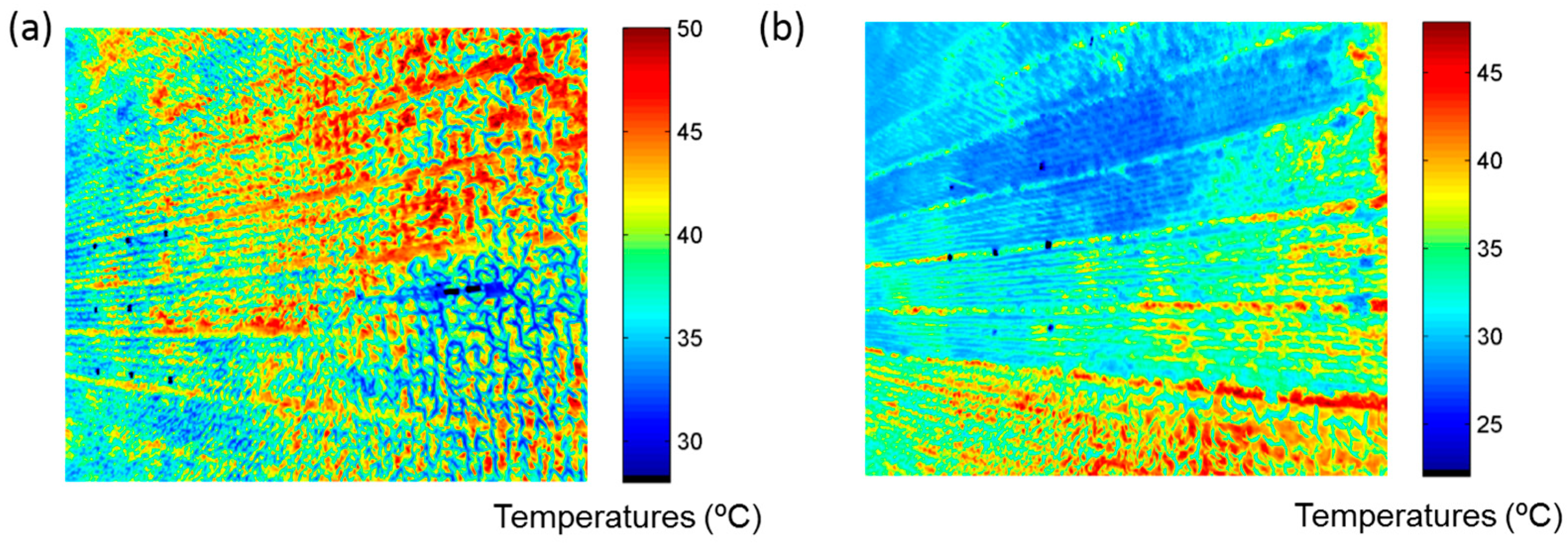
Multi-angle observations were collected via consecutive observations as the WIDAS sensor passed over the area of interest. Targets were observed on multiple occasions to form a series of images. The observation angle varied with the relative position between the flight and the target. After observation, the thermal camera was calibrated using a Blackbody Mikron340 at the State Key Laboratory of Remote Sensing Science. The atmospheric correction of the airborne dataset was conducted with the moderate resolution atmospheric transmission (MODTRAN) code, version 4.0, and synchronous radio soundings [40]. After the geometric correction, the spatial resolutions of the thermal band were resampled to 5.0 m. We selected a study area with a size of 100.0 m × 100.0 m, where another thermal camera simultaneously measured the brightness temperatures of the leaves and soil. Observations of the study area were acquired by aggregating all of the pixels. For the dataset measured with the tower crane, only the downward-directed atmospheric effect was considered using the measured effective atmospheric temperature, because the WIDAS sensor was suspended only 10.0 m above the surface. Figure 8a,b shows the observed TIR images over maize and wheat canopies. In the experiment, the azimuth angle corresponded to the sensor approaching and receding for two observations. In this paper, we used the two observations with azimuth angles of 120–300° for the orchard canopy and four observations along two azimuth angles (0–180° and 90–270°) for both maize and wheat canopies. Unfortunately, because the images in the visible band were not successfully calibrated, only two algorithms (FR97 and GCI) were used.
The leaf and soil material emissivity values were measured using an ABB BOMEM MR304 Fourier transform infrared spectrometer and retrieved using the iterative spectrally smooth temperature and emissivity separation (ISSTES) algorithm [41]. The leaf and soil brightness temperatures in the validation were acquired from TIR images that were simultaneously captured using an FLIR S60 thermal camera during the flights. The component brightness temperatures were classified and converted to radiative temperatures using the atmospheric long-wave radiation and the component material emissivity values [42]. We acquired the component temperatures for the dataset measured with the tower crane platform using a similar method but from the same image for directional observations, because the at-nadir spatial resolution was less than 0.02 m.
Accurate gap frequency and clumping index information can be acquired from the simulated dataset. In contrast, for an actual inversion task, obtaining the actual directional clumping index is difficult. According to the aforementioned comparisons, we used the average clumping index of 0.80 in the maize canopies. Considering the row structure of the orchard and wheat canopies, the estimation algorithm from Yan et al. [37] was used for the gap frequency.
4.3. Results
The leaf and soil temperatures were retrieved using VZAs of approximately 5 and 45° (Table 3). The results retrieved using the GCI algorithm agreed well with the measured values, especially for the wheat and orchard canopies. For maize canopies, similar soil temperatures were retrieved using the GCI and FR97 algorithms. In contrast, the leaf temperatures retrieved by the GCI algorithm were slightly lower than those retrieved by the FR97 algorithm. This difference is likely due to the average clumping index used in the GCI algorithm.
For the wheat canopies, the leaf temperatures retrieved using the GCI algorithm were higher than those using the FR97 algorithm with the sensor-toward angles of 0 and 180°, which corresponded to the cross-row direction. In general, larger angular variations in the measurements occur in the cross-row direction. Therefore, lower leaf temperatures and higher soil temperatures may be retrieved if the estimated CEE in a homogeneous canopy was used in this case. The same conditions apply to the orchard canopy.
4.4. Discussion
Surface temperature validation is difficult because of the strong temporal and spatial variations in large-scale pixels. It should be mentioned that relatively few measurements were used for the validation, although the GCI algorithm appears to perform better and has lower RMSEs. In this study, scenes of turbid vegetation, regularly planted crops and randomly distributed forest were constructed to evaluate the proposed inversion algorithm, but limited measured data were used. Although the simulated and measured results both indicated that using the clumping index can improve the inversion results, the directional anisotropy in a large-scale pixel may be significantly different from that in a small-scale area. For instance, the row structure may play an important role in the directional anisotropy of near-surface measurements. However, at a low spatial resolution, its effect may decrease because of a mixture of plots with different row directions [43]. Therefore, future work should focus on temperature inversion using satellite-based thermal images directly. In addition, in the inversion process, only two VZAs, i.e., nadir and forward 55°, were used, in order to remain consistent with the setting of the along-track scanning radiometer (ATSR) sensor. If additional observations are used, more detailed temperature information about a pixel could be retrieved.
In this paper, we propose a simple inversion procedure for leaf and soil surface temperatures that uses a clumping index. The average clumping index was applied for crop and dense forest canopies. For sparse forest canopies, the average clumping index cannot accurately reproduce the angular variation in the CEE, therefore the directional clumping index was used. The geometric optics theory was adopted to estimate the directional clumping index. Using a similar geometric optics theory, Pinheiro et al. [44] analyzed the angular effect of the advanced very high resolution radiometer (AVHRR) LST data over Africa. Therefore, applying such geometric optics theories to component temperature inversion is possible. In fact, the gap frequency of sparse forest and row-planted crops calculated using Equations (10) and (12) can directly replace in Equations (5)–(9). However, we are trying to propose a unified inversion procedure for surface component temperatures by attributing vegetation distribution patterns to the clumping index. In this case, the inversion procedure would become certain, if the clumping index can be retrieved by many existing algorithms in advance.
5. Conclusions
In this paper, we proposed a simple but robust temperature inversion algorithm that uses a clumping index for leaf and soil surface temperatures. We also recommended several existing algorithms for estimating the average and directional clumping indexes for different landscapes, including row-planted and regular-planted crops and forest. Evaluations were conducted based on both simulated and measured datasets. The results indicated that the GCI algorithm was very promising, with RMSEs less than 1.0 °C relative to the simulated dataset. However, the inversion algorithm appears to be highly sensitive to the LAI. When an LAI bias of ±0.5 was imposed, the RMSEs of the retrieved results were as large as approximately 2.0 °C. The measured datasets over orchard, maize and wheat canopies were also used for validation, and similar results were obtained. Therefore, using the clumping index can improve inversion results.
Currently, the sea and land surface temperature radiometer (SLSTR) aboard the Sentinel-3A satellite, which was launched on 16 February 2016, can be used to obtain quasi-real-time observations with two viewing angles of approximately nadir and oblique (55°) [45]. This sensor represents a continuation of the ATSR sensor series and makes it possible to invert large-scale component temperatures from operational satellite data. We recommend the GCI algorithm as a good foundation for future satellite-based applications for two reasons: (1) its robust performance over both crop and forest scenes and (2) its straightforward form.
Acknowledgments
This work was supported by the National Natural Science Foundation of China (41501366, 41571359, 41571357, 41571329 and 41671366), and the Major State Basic Research Development Program of China (2013CB733401). The ground data and airborne observations used in this study were obtained from the HiWATER and Huailai experiments, and the authors thank all of the scientists, engineers, and students who participated in the HiWATER and Huailai campaigns.
Author Contributions
Biao Cao, Yongming Du, Wenjie Fan, Qing Xiao and Qinhuo Liu convinced and designed the experiments. Zunjian Bian, Biao Cao and Wenjie Fan performed the experiments. Zunjian Bian analyzed the data. Biao Cao, Hua Li, Yongming Du, Wenjie Fan and Lisheng Song participated in the discussion. Zunjian Bian wrote the manuscript. Yongming Du contributed to the conclusion and revision.
Conflicts of Interest
The authors declare no conflict of interest.
References
- Bastiaanssen, W.G.; Molden, D.J.; Makin, I.W. Remote sensing for irrigated agriculture: Examples from research and possible applications. Agric. Water Manag. 2000, 46, 137–155. [Google Scholar] [CrossRef]
- Seelan, S.K.; Laguette, S.; Casady, G.M.; Seielstad, G.A. Remote sensing applications for precision agriculture: A learning community approach. Remote Sens. Environ. 2003, 88, 157–169. [Google Scholar] [CrossRef]
- Wan, Z.; Dozier, J. A generalized split-window algorithm for retrieving land-surface temperature from space. IEEE Trans. Geosci. Remote Sens. 1996, 34, 892–905. [Google Scholar]
- Wan, Z.; Li, Z.-L. A physics-based algorithm for retrieving land-surface emissivity and temperature from eos/modis data. IEEE Trans. Geosci. Remote Sens. 1997, 35, 980–996. [Google Scholar]
- Gillespie, A.; Rokugawa, S.; Matsunaga, T.; Cothern, J.S.; Hook, S.; Kahle, A.B. A temperature and emissivity separation algorithm for advanced spaceborne thermal emission and reflection radiometer (aster) images. IEEE Trans. Geosci. Remote Sens. 1998, 36, 1113–1126. [Google Scholar] [CrossRef]
- Li, Z.L.; Tang, B.H.; Wu, H.; Ren, H.; Yan, G.; Wan, Z.; Trigo, I.F.; Sobrino, J.A. Satellite-derived land surface temperature: Current status and perspectives. Remote Sens. Environ. 2013, 131, 14–37. [Google Scholar] [CrossRef]
- Hulley, G.C.; Hughes, C.G.; Hook, S.J. Quantifying uncertainties in land surface temperature and emissivity retrievals from aster and modis thermal infrared data. J. Geophys. Res. 2012, 117, D23. [Google Scholar] [CrossRef]
- Li, H.; Sun, D.; Yu, Y.; Wang, H.; Liu, Y.; Liu, Q.; Du, Y.; Wang, H.; Cao, B. Evaluation of the viirs and modis lst products in an arid area of northwest China. Remote Sens. Environ. 2014, 142, 111–121. [Google Scholar] [CrossRef]
- Kimes, D.S. Effects of vegetation canopy structure on remotely sensed canopy temperatures. Remote Sens. Environ. 1980, 10, 165–174. [Google Scholar] [CrossRef]
- Du, Y.; Liu, Q.; Chen, L.; Liu, Q.; Yu, T. Modeling directional brightness temperature of the winter wheat canopy at the ear stage. IEEE Trans. Geosci. Remote Sens. 2007, 45, 3721–3739. [Google Scholar] [CrossRef]
- Yu, T.; Gu, X.F.; Guoliang, G.L.; LeGrand, M.; Baret, F.; Hanocq, J.F.; Bosseno, R.; Zhang, Y. Modeling directional brightness temperature over a maize canopy in row structure. IEEE Trans. Geosci. Remote Sens. 2004, 42, 2290–2304. [Google Scholar] [CrossRef]
- Norman, J.M.; Kustas, W.P.; Humes, K.S. Source approach for estimating soil and vegetation energy fluxes in observations of directional radiometric surface temperature. Agric. For. Meteorol. 1995, 77, 263–293. [Google Scholar] [CrossRef]
- Kustas, W.P.; Norman, J.M. A two-source approach for estimating turbulent fluxes using multiple angle thermal infrared observations. Water Resour. Res. 1997, 33, 1495–1508. [Google Scholar] [CrossRef]
- Kustas, W.P.; Norman, J.M. A two-source energy balance approach using directional radiometric temperature observations for sparse canopy covered surfaces. Agron. J. 2000, 92, 847–854. [Google Scholar] [CrossRef]
- Song, L.; Liu, S.; Kustas, W.P.; Zhou, J.; Xu, Z.; Xia, T.; Li, M. Application of remote sensing-based two-source energy balance model for mapping field surface fluxes with composite and component surface temperatures. Agric. For. Meteorol. 2016, 230, 8–19. [Google Scholar] [CrossRef]
- Timmermans, J.; Verhoef, W.; van der Tol, C.; Su, Z. Retrieval of canopy component temperatures through bayesian inversion of directional thermal measurements. Hydrol. Earth Syst. Sci. 2009, 13, 1249–1260. [Google Scholar] [CrossRef]
- Menenti, M.; Jia, L.; Li, Z.L.; Djepa, V.; Wang, J.; Stoll, M.P.; Su, Z.; Rast, M. Estimation of soil and vegetation temperatures with multiangular thermal infrared observations: Imgrass, heife, and sgp 1997 experiments. J. Geophys. Res. 2001, 106, 11997–12010. [Google Scholar] [CrossRef]
- Jia, L.; Li, Z.L.; Menenti, M.; Su, Z.; Verhoef, W.; Wan, Z. A practical algorithm to infer soil and foliage component temperatures from bi-angular atsr-2 data. Int. J. Remote Sens. 2003, 24, 4739–4760. [Google Scholar] [CrossRef]
- Li, Z.; Stoll, M.; Renhua, Z.; Li, J.; Zhongbo, S. On the separate retrieval of soil and vegetation temperatures from atsr data. Sci. China Ser. D 2001, 44, 97–111. [Google Scholar]
- Kimes, D. Remote sensing of row crop structure and component temperatures using directional radiometric temperatures and inversion techniques. Remote Sens. Environ. 1983, 13, 33–55. [Google Scholar] [CrossRef]
- Francois, C.; Ottle, C.; Prevot, L. Analytical parameterization of canopy directional emissivity and directional radiance in the thermal infrared. Application on the retrieval of soil and foliage temperatures using two directional measurements. Int. J. Remote Sens. 1997, 18, 2587–2621. [Google Scholar] [CrossRef]
- Colaizzi, P.D.; O’Shaughnessy, S.; Gowda, P.; Evett, S.; Howell, T.; Kustas, W.; Anderson, M. Radiometer footprint model to estimate sunlit and shaded components for row crops. Agron. J. 2010, 102, 942–955. [Google Scholar] [CrossRef]
- Shi, Y. Thermal infrared inverse model for component temperatures of mixed pixels. Int. J. Remote Sens. 2011, 32, 2297–2309. [Google Scholar] [CrossRef]
- Nilson, T. A theoretical analysis of the frequency of gaps in plant stands. Agric. Meteorol. 1971, 8, 25–38. [Google Scholar] [CrossRef]
- Anderson, M.C.; Norman, J.; Kustas, W.P.; Li, F.; Prueger, J.H.; Mecikalski, J.R. Effects of vegetation clumping on two-source model estimates of surface energy fluxes from an agricultural landscape during smacex. J. Hydrometeorol. 2005, 6, 892–909. [Google Scholar] [CrossRef]
- Huang, H.; Qin, W.; Liu, Q. Rapid: A radiosity applicable to porous individual objects for directional reflectance over complex vegetated scenes. Remote Sens. Environ. 2013, 132, 221–237. [Google Scholar] [CrossRef]
- Chen, L.F.; Li, Z.L.; Liu, Q.H.; Chen, S.; Tang, Y.; Zhong, B. Definition of component effective emissivity for heterogeneous and non-isothermal surfaces and its approximate calculation. Int. J. Remote Sens. 2004, 25, 231–244. [Google Scholar] [CrossRef]
- Xu, X.; Fan, W.; Chen, L. Matrix expression of thermal radiative characteristics for an open complex. Sci. China Ser. D 2002, 45, 654–661. [Google Scholar] [CrossRef]
- Sun, K.; Chen, S.-B. Genetic algorithm based surface component temperatures retrieval by integrating modis tir data from terra and aqua satellites. J. Infrared Millim. Waves 2012, 31, 462–468. [Google Scholar] [CrossRef]
- Bian, Z.; Xiao, Q.; Cao, B.; Du, Y.; Li, H.; Wang, H.; Liu, Q.; Liu, Q. Retrieval of leaf, sunlit soil, and shaded soil component temperatures using airborne thermal infrared multiangle observations. IEEE Trans. Geosci. Remote Sens. 2016, 54, 4660–4671. [Google Scholar] [CrossRef]
- Fan, W.; Xu, X. Integrative inversion of land surface component temperature. Sci. China Ser. D 2005, 48, 2011–2019. [Google Scholar] [CrossRef]
- Chen, J.; Black, T. Foliage area and architecture of plant canopies from sunfleck size distributions. Agric. For. Meteorol. 1992, 60, 249–266. [Google Scholar] [CrossRef]
- Ren, H.; Liu, R.; Yan, G.; Li, Z.-L.; Qin, Q.; Liu, Q.; Nerry, F. Performance evaluation of four directional emissivity analytical models with thermal sail model and airborne images. Opt. Express 2015, 23, A346–A360. [Google Scholar] [CrossRef] [PubMed]
- Verhoef, W.; Jia, L.; Xiao, Q.; Su, Z. Unified optical-thermal four-stream radiative transfer theory for homogeneous vegetation canopies. IEEE Trans. Geosci. Remote Sens. 2007, 45, 1808–1822. [Google Scholar] [CrossRef]
- He, L.; Chen, J.M.; Pisek, J.; Schaaf, C.B.; Strahler, A.H. Global clumping index map derived from the modis brdf product. Remote Sens. Environ. 2012, 119, 118–130. [Google Scholar] [CrossRef]
- Li, J.; Fan, W.; Liu, Y.; Zhu, G.; Peng, J.; Xu, X. Estimating savanna clumping index using hemispherical photographs integrated with high resolution remote sensing images. Remote Sens. 2017, 9, 52. [Google Scholar] [CrossRef]
- Yan, B.; Xu, X.; Fan, W. A unified canopy bidirectional reflectance (BRDF) model for row ceops. Sci. China Earth Sci. 2012, 55, 824–836. [Google Scholar] [CrossRef]
- Li, X.; Cheng, G.; Liu, S.; Xiao, Q.; Ma, M.; Jin, R.; Che, T.; Liu, Q.; Wang, W.; Qi, Y. Heihe watershed allied telemetry experimental research (hiwater): Scientific objectives and experimental design. Bull. Am. Meteorol. Soc. 2013, 94, 1145–1160. [Google Scholar] [CrossRef]
- Liu, Q.; Xiao, Q.; Liu, Z.; Li, F.; Peng, J.J.; Li, B. Image processing method of airborne widas sensor in water campaign. Remote Sens. Technol. Appl. 2010, 25, 797–804. [Google Scholar]
- Berk, A.; Anderson, G.P.; Bernstein, L.S.; Acharya, P.K.; Dothe, H.; Matthew, M.W.; Adler-Golden, S.M.; Chetwynd, J.H., Jr.; Richtsmeier, S.C.; Pukall, B. Modtran 4 Radiative Transfer Modeling for Atmospheric Correction; SPIE—The International Society for Optical Engineering: Bellingham, WA, USA, 1999; pp. 348–353. [Google Scholar]
- Borel, C.C. Surface emissivity and temperature retrieval for a hyperspectral sensor. In Proceedings of the IEEE Geoscience and Remote Sensing Symposium 1998, Seattle, WA, USA, 6–10 July 1998; pp. 546–549. [Google Scholar]
- Song, L.; Liu, S.; Zhang, X.; Zhou, J.; Li, M. Estimating and validating soil evaporation and crop transpiration during the hiwater-musoexe. IEEE Geosci. Remote Sens. Lett. 2015, 12, 334–338. [Google Scholar] [CrossRef]
- Cao, B.; Liu, Q.; Du, Y.; Li, H.; Wang, H.; Xiao, Q. Modeling directional brightness temperature over mixed scenes of continuous crop and road: A case study of the heihe river basin. IEEE Geosci. Remote Sens. Lett. 2015, 12, 234–238. [Google Scholar] [CrossRef]
- Pinheiro, A.C.T.; Privette, J.L.; Mahoney, R.; Tucker, C.J. Directional effects in a daily avhrr land surface temperature dataset over africa. IEEE Trans. Geosci. Remote Sens. 2004, 42, 1941–1954. [Google Scholar] [CrossRef]
- Donlon, C.; Berruti, B.; Buongiorno, A.; Ferreira, M.-H.; Féménias, P.; Frerick, J.; Goryl, P.; Klein, U.; Laur, H.; Mavrocordatos, C. The global monitoring for environment and security (gmes) sentinel-3 mission. Remote Sens. Environ. 2012, 120, 37–57. [Google Scholar] [CrossRef]
Figure 1.
Three scenes for the simulated datasets: (a) turbid canopy; (b) regularly planted crops; and (c) randomly distributed forest. In scenes (b) and (c), the plants are composed of a series of horizontally layered and porous facets. The green facets represent the leaves, and the brown facets represent the soil.

Figure 2.
Comparisons of the component effective emissivity (CEE) over turbid (a,b); crop (c,d) and forest (e,f) scenes with leaf area index (LAI) values of 1.0 and 3.0, and a material emissivity profile of 0.99 (leaf) and 0.97 (soil). The colors red, green, cyan and blue are used to differentiate data from different inversion algorithms. Circles and triangles represent leaf and soil components, respectively.

Figure 3.
Temperature difference distribution of retrieved leaf and soil temperatures relative to the reference over turbid (a,b); crop (c,d) and forest (e,f) scenes.
Figure 3.
Temperature difference distribution of retrieved leaf and soil temperatures relative to the reference over turbid (a,b); crop (c,d) and forest (e,f) scenes.
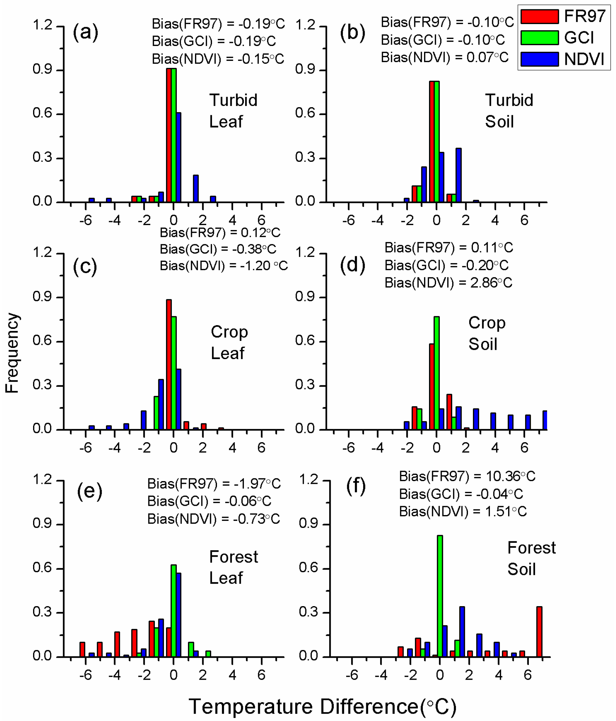
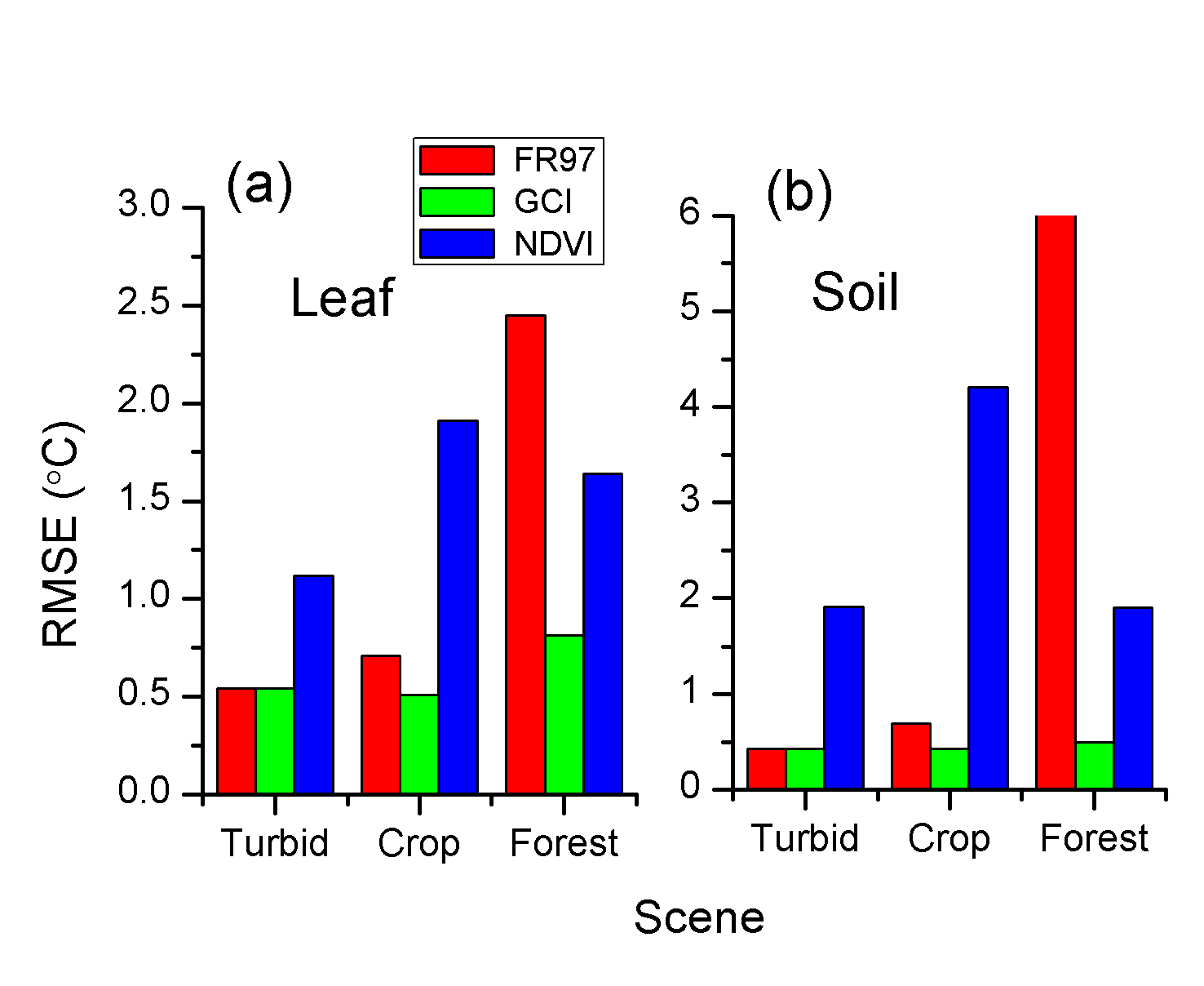
Figure 4.
Root mean squared errors (RMSEs) of retrieved leaf (a) and soil (b) temperatures over turbid, crop and forest scenes. The RMSE for retrieved soil temperatures by the FR97 algorithm over forest scene was approximately 15.0 °C.
Figure 4.
Root mean squared errors (RMSEs) of retrieved leaf (a) and soil (b) temperatures over turbid, crop and forest scenes. The RMSE for retrieved soil temperatures by the FR97 algorithm over forest scene was approximately 15.0 °C.
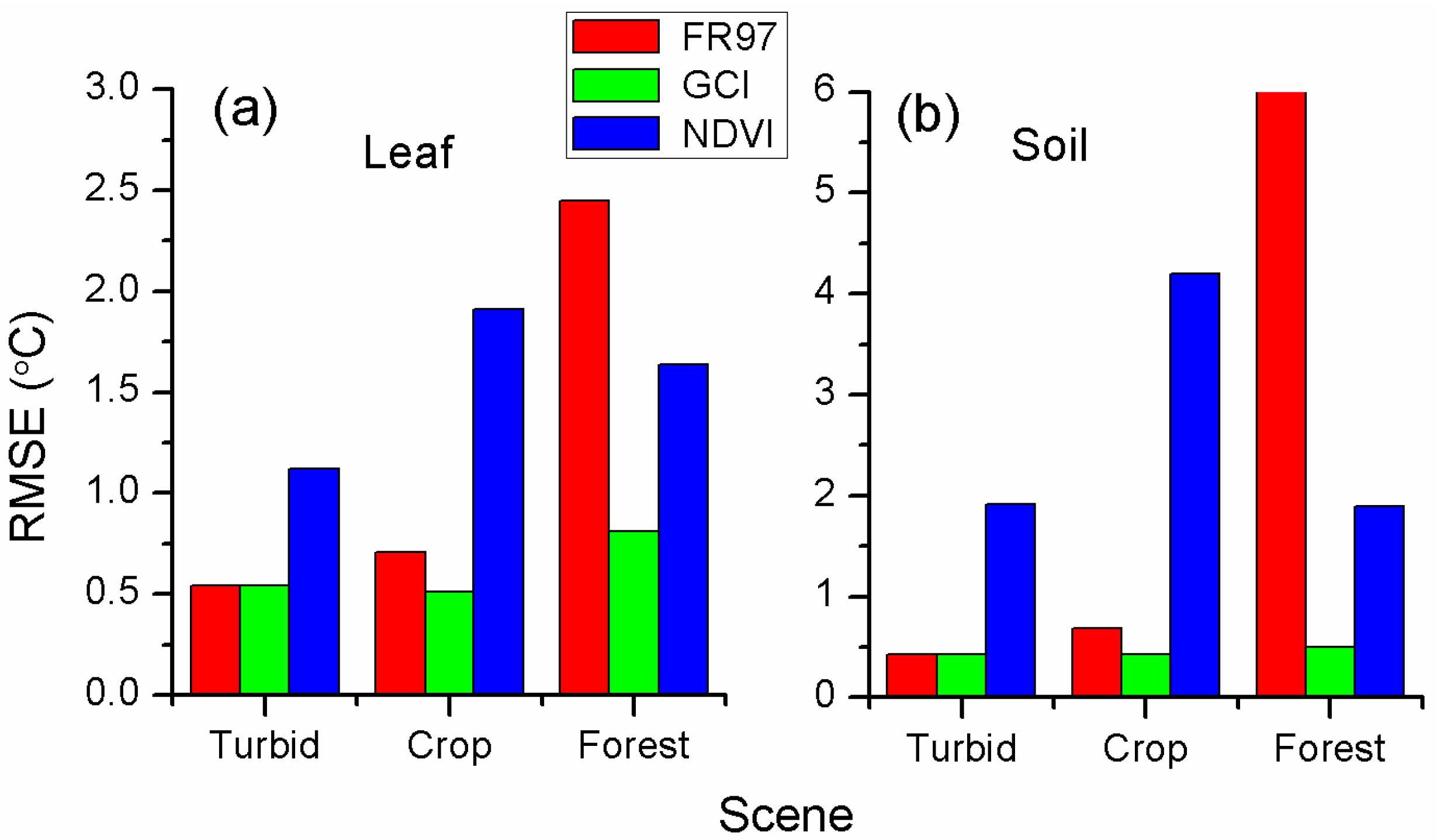
Figure 5.
(a) Average clumping index of crop and forest scenes; The CEE simulated by different algorithms over forest scenes with LAI values of 1.0 (b) and 3.0 (c). Subscripts a and d, respectively, represent the average and directional clumping indexes.
Figure 5.
(a) Average clumping index of crop and forest scenes; The CEE simulated by different algorithms over forest scenes with LAI values of 1.0 (b) and 3.0 (c). Subscripts a and d, respectively, represent the average and directional clumping indexes.

Figure 6.
RMSEs of the retrieved results over crop (a) and forest (b) scenes when different clumping index biases were imposed.
Figure 6.
RMSEs of the retrieved results over crop (a) and forest (b) scenes when different clumping index biases were imposed.

Figure 7.
Retrieved results from the new algorithm over crop (a) and forest (b) scenes, when LAI biases (±0.3, ±0.5) were imposed on LAI values varying from 1.0 to 3.5.
Figure 7.
Retrieved results from the new algorithm over crop (a) and forest (b) scenes, when LAI biases (±0.3, ±0.5) were imposed on LAI values varying from 1.0 to 3.5.

Figure 8.
Thermal images acquired over maize (a) and wheat (b) canopies at the Huailai remote sensing site.
Figure 8.
Thermal images acquired over maize (a) and wheat (b) canopies at the Huailai remote sensing site.


Table 1.
Scenario set.
| Parameter | Unit | Value or Range |
|---|---|---|
| Scene | -- | Turbid, Crop, Forest |
| LAI | -- | 0.5, 1,0, 1.5, 2.0, 2.5, 3.0, 3.5 |
| LIDF | -- | Spherical |
| (red) | -- | 0.057 |
| (red) | -- | 0.042 |
| (red) | -- | 0.164 |
| (NIR) | -- | 0.460 |
| (NIR) | -- | 0.462 |
| (NIR) | -- | 0.244 |
| -- | 0.99, 0.97 | |
| -- | 0.97, 0.93 | |
| VZA | ° | [0, 60] |
| °C | 0, 5, 10, 15, 20 |
Red: red band (670 nm); NIR: near infrared band (870 nm).
Table 2.
Information on the study area.
| Date | Beijing Time | Type | LAI | LIDF | Structure |
|---|---|---|---|---|---|
| 3 August 2012 | 14:00–14:30 | Orchard | 2.4 | Spherical | Row planted; a = 2.5 m; c = 6.0 m; H = 5.0 m; |
| 17 June 2014 | 12:00–14:00 | Maize | 1.2 | Plagiophile | Regularly planted; Spacing = 0.5 m; |
| Wheat | 1.5 | Row plated; a = 0.1 m; c = 0.2 m; H = 0.65 m |
Table 3.
Leaf and soil temperatures from measurements and retrievals.
| Leaf (°C) | Soil (°C) | ||||||
|---|---|---|---|---|---|---|---|
| Scene | Toward Angle (°) | Measured | FR97 | GCI | Measured | FR97 | GCI |
| maize | 180 | 29.3 | 31.7 | 30.3 | 41.2 | 42.5 | 42.4 |
| 0 | 29.4 | 31.3 | 29.0 | 48.2 | 48.5 | 48.1 | |
| 90 | 31.2 | 35.5 | 34.1 | 45.9 | 47.4 | 47.2 | |
| 270 | 32.8 | 34.5 | 32.9 | 46.0 | 46.7 | 46.6 | |
| wheat | 180 | 28.4 | 22.4 | 24.4 | 33.9 | 39.3 | 35.2 |
| 0 | 30.9 | 29.3 | 30.2 | 36.2 | 38.2 | 36.3 | |
| 90 | 32.0 | 32.7 | 31.3 | 42.2 | 41.3 | 41.8 | |
| 270 | 29.1 | 31.0 | 30.1 | 37.7 | 37.2 | 37.5 | |
| orchard | 300 | 29.3 | 26.3 | 28.7 | 46.0 | 46.1 | 45.4 |
| 120 | 30.3 | 27.2 | 29.0 | 48.7 | 45.1 | 45.5 | |
| RMSE | 3.0 | 1.7 | 2.3 | 1.2 | |||
© 2017 by the authors. Licensee MDPI, Basel, Switzerland. This article is an open access article distributed under the terms and conditions of the Creative Commons Attribution (CC BY) license (http://creativecommons.org/licenses/by/4.0/).
Share and Cite
MDPI and ACS Style
Bian, Z.; Cao, B.; Li, H.; Du, Y.; Song, L.; Fan, W.; Xiao, Q.; Liu, Q. A Robust Inversion Algorithm for Surface Leaf and Soil Temperatures Using the Vegetation Clumping Index. Remote Sens. 2017, 9, 780. https://doi.org/10.3390/rs9080780
AMA Style
Bian Z, Cao B, Li H, Du Y, Song L, Fan W, Xiao Q, Liu Q. A Robust Inversion Algorithm for Surface Leaf and Soil Temperatures Using the Vegetation Clumping Index. Remote Sensing. 2017; 9(8):780. https://doi.org/10.3390/rs9080780
Chicago/Turabian StyleBian, Zunjian, Biao Cao, Hua Li, Yongming Du, Lisheng Song, Wenjie Fan, Qing Xiao, and Qinhuo Liu. 2017. "A Robust Inversion Algorithm for Surface Leaf and Soil Temperatures Using the Vegetation Clumping Index" Remote Sensing 9, no. 8: 780. https://doi.org/10.3390/rs9080780
Note that from the first issue of 2016, this journal uses article numbers instead of page numbers. See further details here.