Feasibility of GNSS-R Ice Sheet Altimetry in Greenland Using TDS-1
by
 , , and
Antonio Rius
1,* ,
,
Estel Cardellach
1,
Fran Fabra
1,
Weiqiang Li
1,
Serni Ribó
1 and
Manuel Hernández-Pajares
2 1
Earth Observation Research Group, Institute of Space Sciences (CSIC/IEEC), Barcelona 08193, Spain
2
UPC-IonSAT, IEEC-CTE-CRAE, Universitat Politècnica de Catalunya, Barcelona 08034, Spain
*
Author to whom correspondence should be addressed.
Remote Sens. 2017, 9(7), 742; https://doi.org/10.3390/rs9070742
Submission received: 19 May 2017
/
Revised: 11 July 2017
/
Accepted: 13 July 2017
/
Published: 19 July 2017
Abstract
:Radar altimetry provides valuable measurements to characterize the state and the evolution of the ice sheet cover of Antartica and Greenland. Global Navigation Satellite System Reflectometry (GNSS-R) has the potential to complement the dedicated radar altimeters, increasing the temporal and spatial resolution of the measurements. Here we perform a study of the Greenland ice sheet using data obtained by the GNSS-R instrument aboard the British TechDemoSat-1 (TDS-1) satellite mission. TDS-1 was primarily designed to provide sea state information such as sea surface roughness or wind, but not altimetric products. The data have been analyzed with altimetric methodologies, already tested in aircraft based experiments, to extract signal delay observables to be used to infer properties of the Greenland ice sheet cover. The penetration depth of the GNSS signals into ice has also been considered. The large scale topographic signal obtained is consistent with the one obtained with ICEsat GLAS sensor, with differences likely to be related to L-band signal penetration into the ice and the along-track variations in structure and morphology of the firn and ice volumes. The main conclusion derived from this work is that GNSS-R also provides potentially valuable measurements of the ice sheet cover. Thus, this methodology has the potential to complement our understanding of the ice firn and its evolution.
1. Introduction
Greenland and Antarctica hold about 99 percent of the Earth’s total freshwater ice. Sea level would rise by the order of several tens of meters if these ice sheets were to ever melt [1,2]. Even under a partial loss of these enormous ice masses, coastal areas would suffer significant impacts. Recent studies state that mass loss from the Greenland ice sheet currently accounts for ∼10 percent of the observed global mean sea level rise [3], and that some of its glaciers are melting and retreating rapidly [4]. There is growing evidence that mass loss from the Antarctic ice sheet is also accelerating [5]. Furthermore, some melting events affect large areas of the ice sheet surfaces within a short time span, such as the extreme event recorded in July 2012, when for one day about 98 percent of Greenland’s ice sheet presented signs of surface melting [6]. This possibility requires a precise knowledge of the mass balance of the large ice sheets in Greenland and Antarctica, that is, the difference between the precipitation over the sheets (essentially snowfall) and the effect of different ice loss mechanisms: ablation (evaporation of the ice), surface melt, calving at the interface with the ocean, and melting from contact with the warmer ocean.
One of the techniques to study the ice mass balance uses measurements of the ice elevation taken from satellite altimeters. The changes of the ice topography are evaluated over time to infer the volumetric variation of the ice sheets. The ice sheets topography is also relevant to other scientific questions, such as their influence on weather and climate. For instance, high altitude topographic features of ice caps can alter storm tracks and they also play a role in the development of dry and cold down-slope winds that reach hurricane forces. These dry cold winds over the ice surface can lead to ablation of the ice, which in turn modifies its topography.
Two distinct types of sensors are used to obtain ice topography from space: dedicated radar and laser altimeters (e.g., NASA’s ICESat [7] and ESA’s Cryosat-2 [8]) and opportunistic radar altimeters (e.g., ESA’s ERS-1, ERS-2, ENVISAT). While the dedicated instruments are optimized to perform altimetry over sea ice and ice sheets, with fine spatial resolution and capability to recover steep slopes of the terrain, the opportunistic ones were not originally intended for ice applications. Nevertheless, analysis of their data has contributed to expanding the time series of ice topography and mass balance studies back to times before dedicated missions were launched. The precision of these instruments ranges from decimeters to several meters, and it depends on the employed technique and slope of the terrain [9]. ICESat stopped data acquisition in 2010 and Cryosat-2 is still active, but it has doubled its designed lifetime. Current or planned opportunistic altimetric missions include ESA’s Sentinel-3 and NASA/CNES Jason-n series, as well as NASA’s SWOT. Unfortunately, none of them fully covers the Poles.
In this study we present the preliminary performance of a new opportunistic ice topographic technique. The altimetric retrievals are based on bi-static radar measurements of the delay between the location of a transmitter of the Global Navigation Satellite System (GNSS), the icy reflecting cover and a low Earth orbiter able to capture GNSS signals reflected off the Earth. This technique is called GNSS reflectometry (GNSS-R), and it can be done (a) by cross-correlating the well-known available codes transmitted by the GNSS satellites (e.g., the Global Positioning System–GPS–C/A codes) with the reflected signals or (b) by cross-correlating the received direct signals with the reflected signals. The former approach, named conventional GNSS-R (cGNSS-R), presents coarse delay resolutions as determined by the narrow bandwidth of the public codes. The latter approach, named interferometric GNSS-R (iGNSS-R) makes use of the whole transmitted bandwidth, including the broader bandwidth encrypted codes, of greater delay resolution [10]. Traditionally, cGNSS-R has been linked to ocean scattering applications, such as in the NASA mission CYGNSS [11], which do not require a delay resolution as fine as in altimetric applications. The iGNSS-R was conceived for ocean altimetric purposes with precision assessed to be 2 to 4 times better than those obtained by the conventional cGNSS-R approach [12,13].
2. GNSS-R and the TDS-1 Reflectometry Instrument
Currently, there is no spaceborne experiment to check the actual performance of the iGNSS-R altimetry over ice sheets. The ESA mission GEROS-ISS [14], which plans to include the iGNSS-R technique for ocean altimetry applications, will not cover the main ice sheets because of the low inclination of its orbit. On the other hand, the UK TDS-1 satellite, a British technological demonstration satellite, carries a payload that takes cGNSS-R measurements during two days out of eight [15]. The TDS-1 satellite was placed into a quasi Sun synchronous orbit with altitude of 635 km and an inclination of , and thus able to cover the whole Greenland sheet and most of Antarctica.
Because of the implementation of the conventional approach, its altimetric precision is expected to be much coarser than the corresponding to an iGNSS-R instrument. Despite this limitation, in this study we aim to test its performance over the Greenland ice sheet, to be understood as the lowest performance bound of the technique for ice sheet topography (Figure 1). Reference [16] reported altimetry over Greenland using GPS reflected signals found in GPS radio-occultation data collected aboard the German CHAMP satellite. As in UK TDS-1, the observables were also based on conventional GNSS-R, but unlike UK TDS-1 data, they were obtained at very low elevation angles (close to tangential reflection, elevation angles of 0–1), resulting in purely coherent scattering. In that case, the phase of the electromagnetic field was tracked and used to conduct the altimetry (phase-delay altimetry technique). We could also expect a certain degree of coherence in the signals reflected off Greenland ice sheet, as we found in a ground based experiment over the Antarctica ice sheet, around Concordia station, where we applied radio-holographic techniques to sense sub-surface snow layers [17]. However, the TDS-1 data available over Greenland were integrated incoherently aboard the satellite, and the phase information was lost. Therefore, in this study we can only deal with group-delay altimetric techniques.
Data captured by the TDS-1 GNSS-R instrument, hereinafter TDS-1 data, were made publicly available in March 2015 [20]. The main product is a large set of Delay Doppler Maps (DDM), defined as the power of the correlator output as a function of the applied delay and Doppler f offsets with respect to a reference. A DDM is provided in a rectangular window of the correlation space , with dimensions (128 lags, 10,000 Hz). This window is tiled with cells of dimensions (1 lag, 500 Hz).
This data set has been analyzed by different groups to research the remote sensing possibilities offered by the spaceborne GNSS-R technique. For instance, references [15,20,21,22] focus on system aspects of TDS-1. The reader is referred to these references for the details of the TDS-1 mission. Sea surface applications are reported in [23] for scatterometry. Soil moisture applications of TDS-1 are given in [24,25] and the ionosphere is studied in [26].
TDS-1 group-delay spaceborne altimetry has been reported over ocean and sea ice surfaces. Over smooth sea ice in the Hudson Bay the reported precision is 0.96 m in 0.5 s and 3.5 km sampling [27]. Over open ocean, it is reported in [28] that the group-delay cGNSS-R precisions of the order of 7 to 8 m in 1 s observations. High accuracy in sea ice detection and altimetry have been obtained using DDM observables through investigating the signatures of the DDM in [27,29,30,31], and the sea water-ice transition has been detected using radar images reconstructed from the DDMs in [32]. However, the altimetric performance over the continental ice sheet using the group-delay of the reflected signal has never been reported.
Our study aims to expand the list of applications to cover a different objective: the feasibility of near-nadir group-delay altimetric capacity of GNSS-R over ice sheets.
3. Data Set and Models Used in This Study
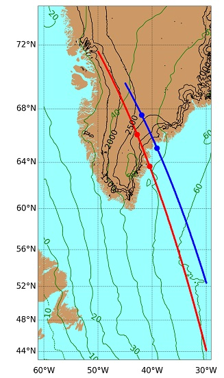
We have analyzed two sets of TDS-1 DDMs gathered on 26 and 27 January 2015, with specular points over the Ocean and Greenland. In Figure 1 we have represented the specular points corresponding to these sets. In this case we should consider three different scattering mechanisms [33]: surface scattering on the sea surface and the ice sheet, volume scattering over the ice, and possible multipath when large changes in the slopes of the reflecting surface are present. Consequently, in each track we distinguish three zones, from South to North: sea, topographic step (strong gradient) and ice, depending on the position of the specular point. The points along the step will not be discussed here, because of the difficulties in modeling such reflections.
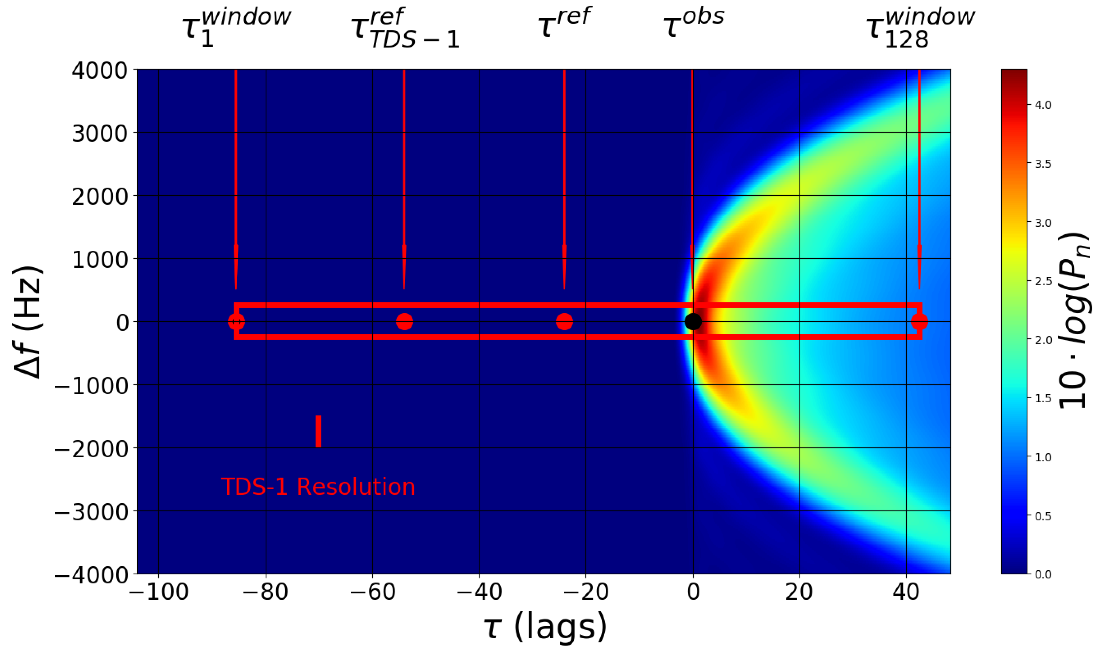
In Figure 2 we present the main elements needed to establish the relation between the TDS-1 observables and the observables as used in this paper. The size of one cell is indicated in the figure as a small red rectangle. In our study we will only use the Doppler slice corresponding to , shown in the figure as a red long rectangle. The power waveforms represented in Figure 2 are normalized using , where is the mean value of P where there is no signal. The quantity represents the observable delay assigned to each power waveform, defined, in the present study, as the delay where its derivative is maximum [34,35]. The point is the TDS-1 reference point. Then the quantity defined as
contains the observational information to correct the model assumptions used in the definition of .
Because the main intended application of the TDS-1 only involves the study of the shape of the power DDMs, the computation of is based on simplified algorithms, and discrepancies on the order of magnitude of 15 m and 200 Hz are expected, as explained in [20]. In fact, this reference suggest recalculation of this quantity, when better accuracy is needed for other applications.
In this study we use a different reference . The main differences with respect to are: (a) we suppose that the specular points are located either in the EGM2008 [18] or in the NSIDC GLAS/ICESat digital elevation model [9] , and (b) to compute the specular point we consider the position of the transmitter, taking into account the signal transit time, and its velocity. In our case, the ellipsoidal longitude and latitude of the specular point are those corresponding to one reflection on the WGS84 ellipsoid, and the ellipsoidal height h is either an interpolated value of the EGM2008 model, when the specular point is over the sea, or otherwise (NSIDC) GLAS/ICESat. Taking into account these considerations, we define our observed delays as:
The characteristics of the sea scattering could be interpreted using the Zavorotny-Voronovich model [36], while for the ice sheet case the surface-volume scattering model described in [37] could be used. Both models correspond to GNSS signals, and are expressed as the convolution product of two functions, one representing the power waveform of the unscattered signal , which is also known as Woodward Ambiguity Function, and the other describing the contribution to the building of the waveform of the elemental scatterers, located in the surface or distributed in the volume:
The model functions correspond to the primary observables used to estimate the observed delays .
3.1. Additional Model Components
In addition to the geometrical model considered above to build our observables, we have included other effects whose magnitudes are on the order of few meters: tidal, tropospheric and ionospheric.
The tidal delays for the specular points over the ocean have been modeled by means of the Oregon State University Tidal Inversion Software (OTIS) [38] and using the tidal regional solution for the Atlantic Ocean (2008), with data assimilated from spaceborne altimeters.
The tropospheric delays (in meters) are computed using a first order Saastamonien model supplemented with a simple mapping function [39]:
where is the standard atmospheric pressure at height h, and i is the incidence angle.
The ionospheric delays experienced by the reflected signal have been estimated by means of the Global Ionospheric Maps (GIM) of Vertical Total Electron Content (VTEC) [40], at 5 deg × 2.5 deg × 15 min of resolution in longitude, latitude and time (see this reference for a discussion on the performance of this model in the context of the International GNSS Service (IGS)). In this case the ionospheric delays were moderate, but it should be noted that the ionospheric delays could be one order of magnitude larger in the case of major geomagnetic storms affecting high-latitude regions.
Estimates of these three effects are shown in Figure 3. Other components regularly used in radar altimetry or space geodesy (e.g, ocean and atmospheric loading, surface slope, etc.) have not been considered in this study given that their corresponding delays, in the sea or ice regions, are much smaller than the uncertainty of our measurements.
3.2. Expected Delay Precision
For the sea case, where the speckle noise is reduced by incoherent averaging of a large quantity of independent power waveforms, reference [10] provides an expression for the estimation of the standard deviation of the delay as
where and are the mean values of the signal part of the waveform and its derivative, is the signal to thermal noise ratio at the observation point, and is the number of independent waveforms taken during the incoherent integration interval.
For the spaceborne scenario, the coherent time of the reflected C/A code signal is expected to be ∼1 ms [41] which means that the TDS-1 one-shot power waveforms are essentially uncorrelated.
The first fraction in (5), which can be computed from the measured waveform, or through theoretical simulation, can be taken as 120 m for the spaceborne case. Considering an incoherent average time of 1 s, i.e., , and ( values from both data and models agree on this approximate value), the expected uncertainty in the delay measurements is m.
As mentioned before, and based on the findings in [17], we can expect a slightly more coherent reflection process over the smooth ice sheets. Nevertheless, as it is predicted by the model explained in reference [37], the volumetric scattering drives the shaping of the waveform. Overall, the data show that levels over both sea and ice sheets are of the same order of magnitude and as a consequence we can expect similar levels of uncertainty.
3.3. Selected Waveforms over Greenland
As mentioned earlier, we have selected two sets of TDS-1 waveforms obtained over Greenland. The selection criteria were: (a) tracks obtained in two consecutive days -26 and 27 January 2015-, (b) tracks transmitted by the same GPS satellite -PRN 31-, (c) tracks with relatively small incidence angles and (d) high antenna gain toward the nominal specular position. These criteria were chosen to produce good quality data, in very similar conditions, and to facilitate comparisons. Only two tracks fulfilled these conditions among the TDS-1 data. Table 1 summarizes the relevant parameters defining both data transects.
In Figure 4 we have represented, in two panels, the normalized power waveforms , in dB, as a function of the second of the day t and the correlator lag for both days. To facilitate the interpretation of the power waveforms, we include in each panel the modeled delay , here understood as the delay with respect to an hypothetical reflection off the reference ellipsoid WGS84. These modeled delays are derived assuming that the sea surface elevation corresponds to the EGM 2008 and the ice surface elevation corresponds to the topography given by NSIDC GLAS/ICESat. Note (a) the nearly linear variation of the peak delay of the sea waveforms-probably related to the open loop nature of the TDS-1 tracking, uncertainties in the determination of the transmitter trajectory or other instrumental causes, (b) the evident similarity between the time evolution of and the peak delays of the ice waveforms, and (c) the reduced number of waveforms visible in the topographic step region, due to the limitations of the model used to track the reference point.
As it has been indicated in Equation (3), the power waveforms could be expressed as the convolution product . In reference ([42], p. 143), it is shown that the variance of this should be the sum of the variances of the two factors and . Because in our case is fixed, the variance of the power waveform will be a measure of the scattering. As indicator of such variance, we use the 3 dB widths of the power waveforms. In each panel of Figure 4 we have included these quantities, which are a source of information of the reflecting media. The systematic difference between sea and ice sheet waveform widths will produce different bias in the determination of the delays as explained in reference [35].
4. Results
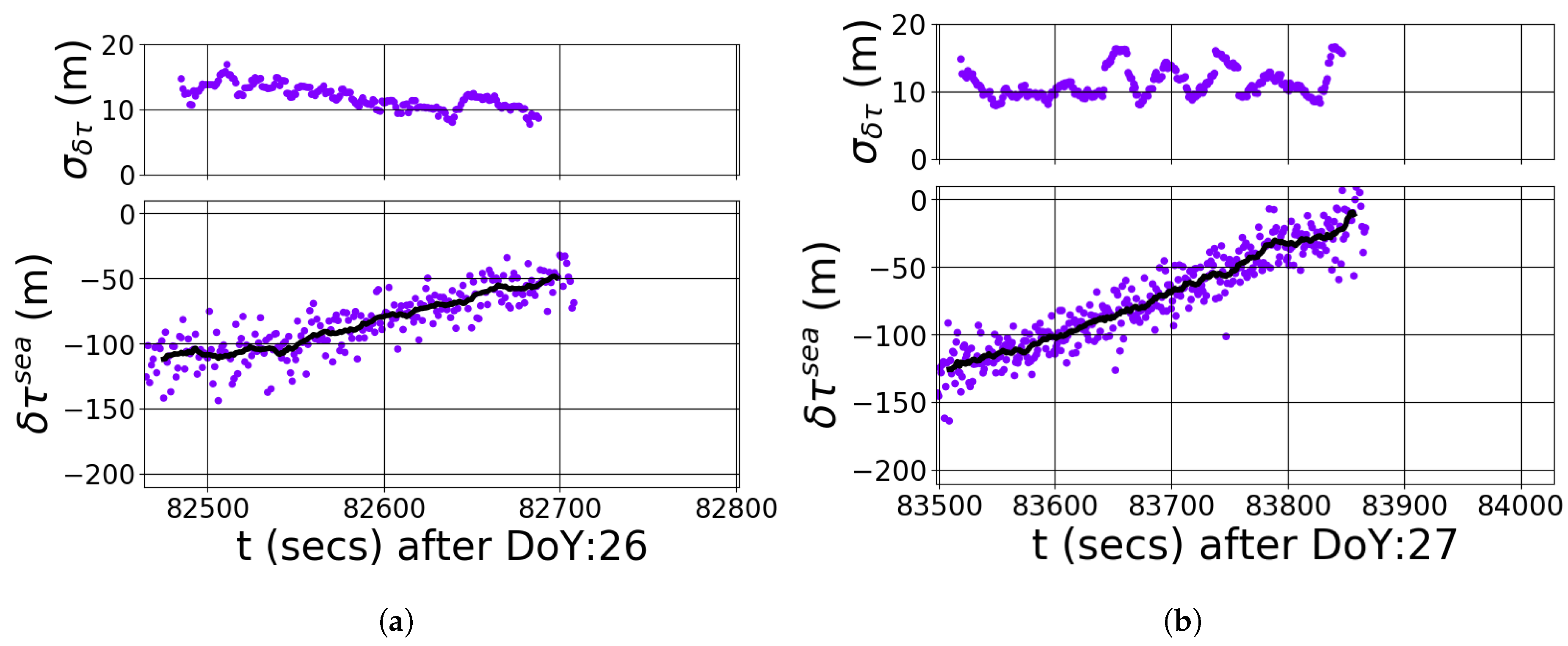
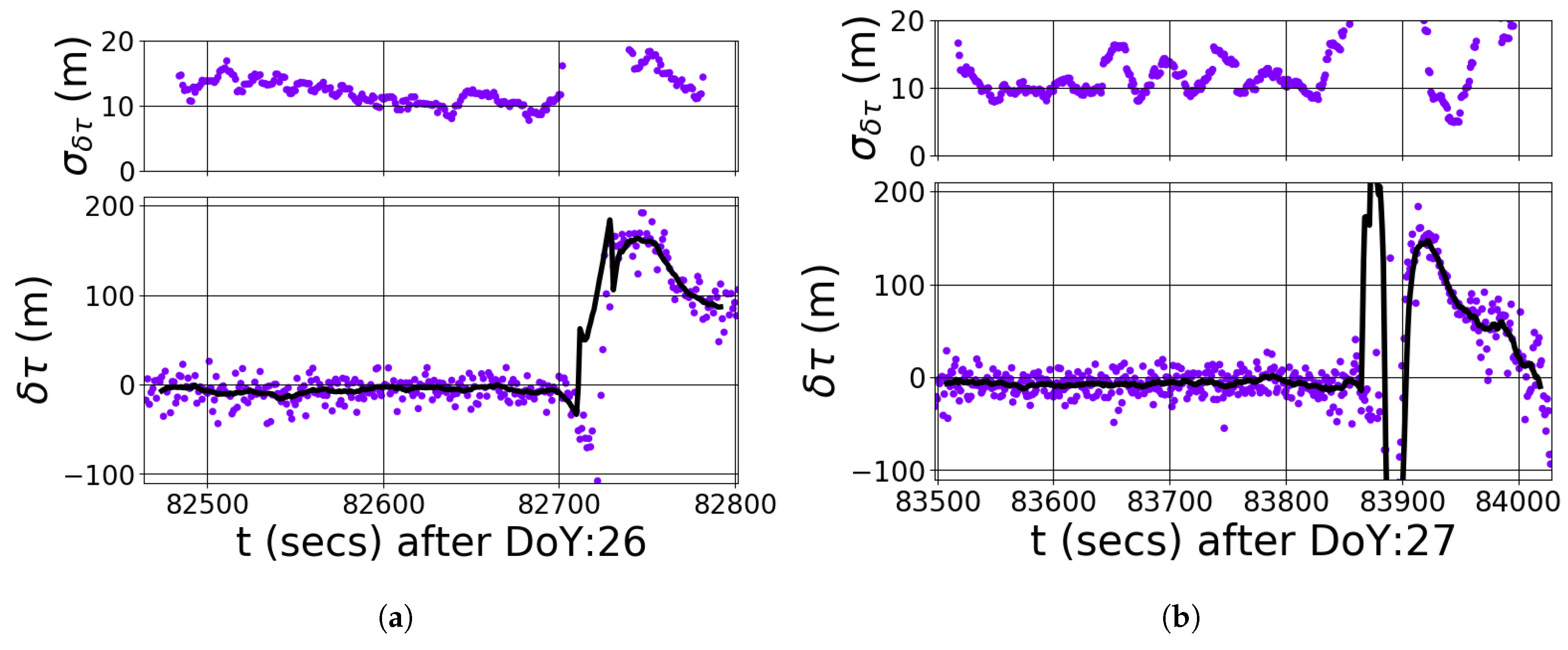
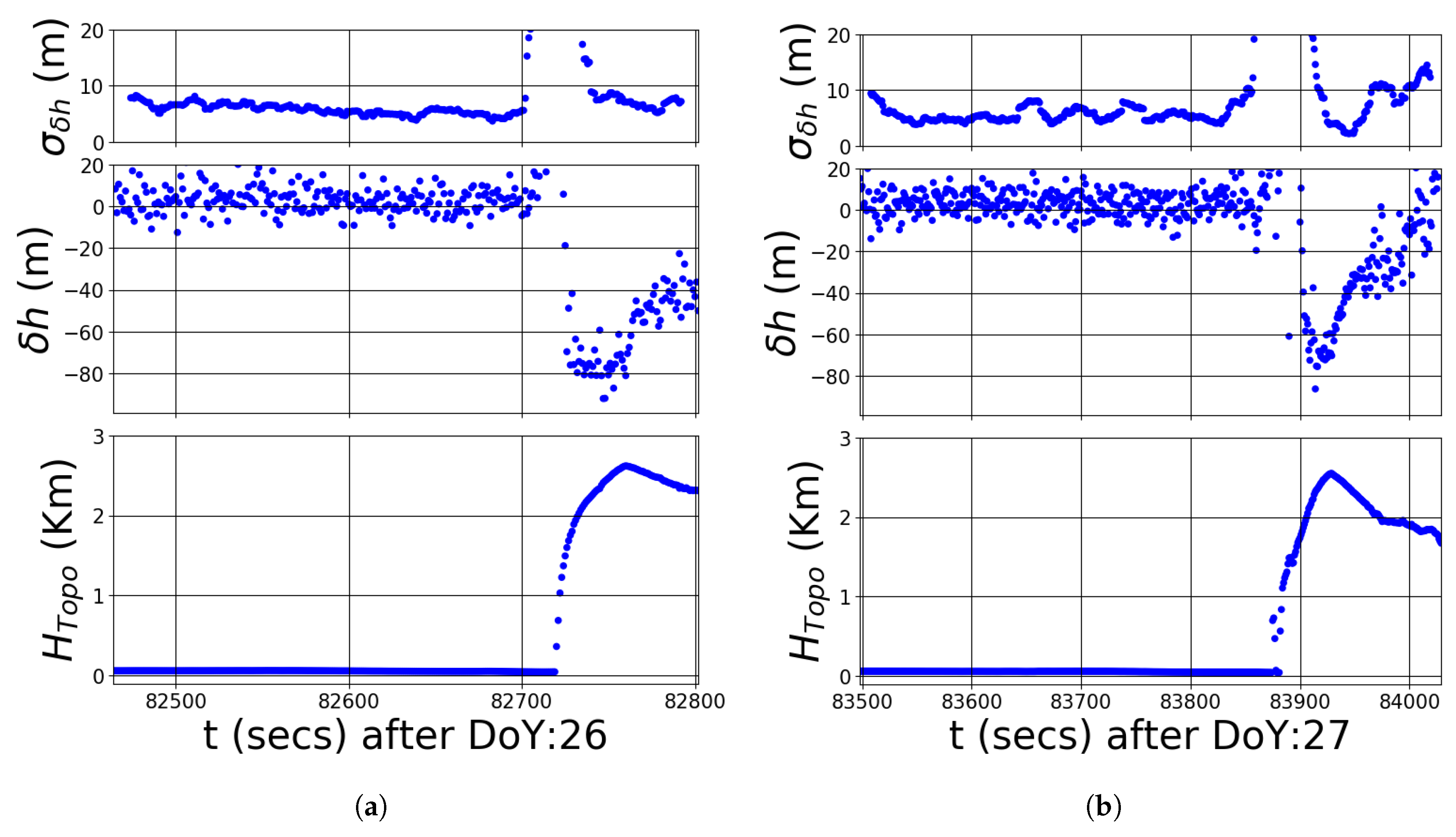
In Figure 5 we have represented the observed delays and their standard deviation over the sea section. These data over the sea have been used to estimate the nearly linear variation of the observed sea delays, unexplained by any geophysical phenomena. We consider these variations as observational nuisance effects to be calibrated. We have extrapolated these variations to all the observation interval, and we have removed this variation to all observations (including those over the ice sheets). The corresponding calibrated observations are presented in Figure 6. From these quantities we derive the apparent height variation computed as
which are represented in Figure 7. The use of the superscript apparent is introduced here to express that in Equation (6) we have not taken into account the refractive index of the ice, i.e., it is assumed that the signal travels through the air solely–no penetration into the ice has been considered.
5. Discussion
If we assume that the extra delay is due to the ice sheet scattering, we need to account for the actual refractive index of the ice. In this case, the vertical distance of the mean locus of the backscatter will be referred as effective height instead of apparent height. We introduce here the term effective height to avoid the use of penetration depth, which, as noted in reference [43], has different definitions in the existing literature.
An approximate relation between apparent heights and its effective counterpart could be obtained assuming that (a) the complex dielectric constant is uniform within the ice sheet, (b) its imaginary component is negligible, and (c) its refractive index is . A signal entering to the ice sheet, from the air () with an incidence angle will be refracted into the direction defined by the Snell’s Law as
Consequently, for a signal entering with an incidence angle i, the relation between the effective height and its apparent counterpart could be written as:
where the mapping F is defined as:
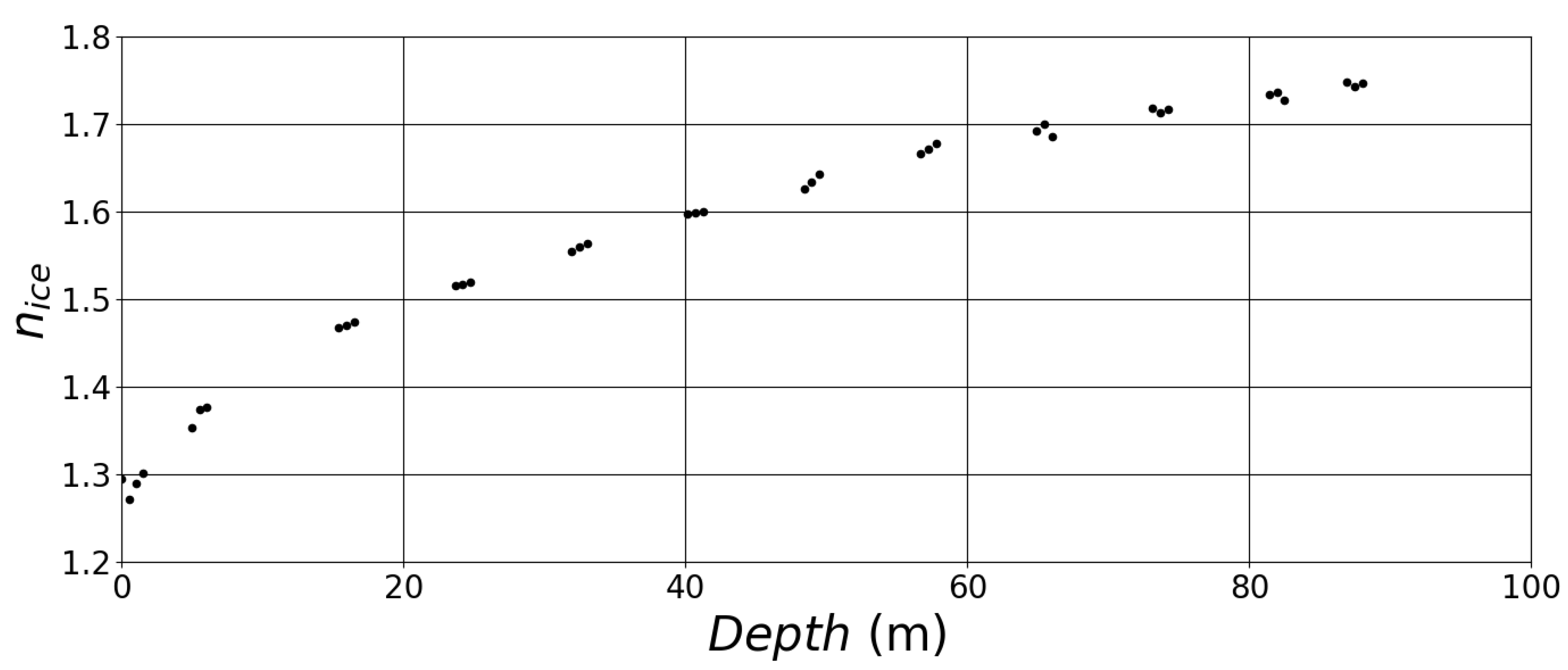
Reference ([44], p. 848) explains that the refractive index within the ice sheet is a function of its depth, being a weighted mean of air () and pure ice ( in the microwave region) refractive indices. To have an order of magnitude value of the expected refractive index in the Greenland ice sheet, we show in Figure 8 a profile of , based on Table 4 of reference [45]. They obtained this as a result of the analysis of data obtained from one of the firn cores drilled down to 88.55 m in the North Greenland Eemian Ice Drilling (NEEM) camp, northwest Greenland at an elevation of 2450 m. These profiles correspond to dry snow, which presents different structure and density profiles than ice in percolation zones. For example, reference [46] shows ice density profiles varying from 600 kg/m to 900 kg/m in the upper 35 m of the firn. According to reference [44], this range of densities corresponds to refractive indexes between ∼1.49 and ∼1.76, nearly 0.2 units higher than the ones in Figure 8.
Reference [47] shows penetration depths up to 120 m in Greenland at L Band. Then, from Figure 8, we take as a representative value for our L-band case. Taking into account the limited range of incidence angles of our observations (see Table 1) and the uncertainties associated to our choice of , we have approximated Equation (9) with the constant . The corresponding effective heights computed using Equation (8) are indicated in the left panel of Figure 9.
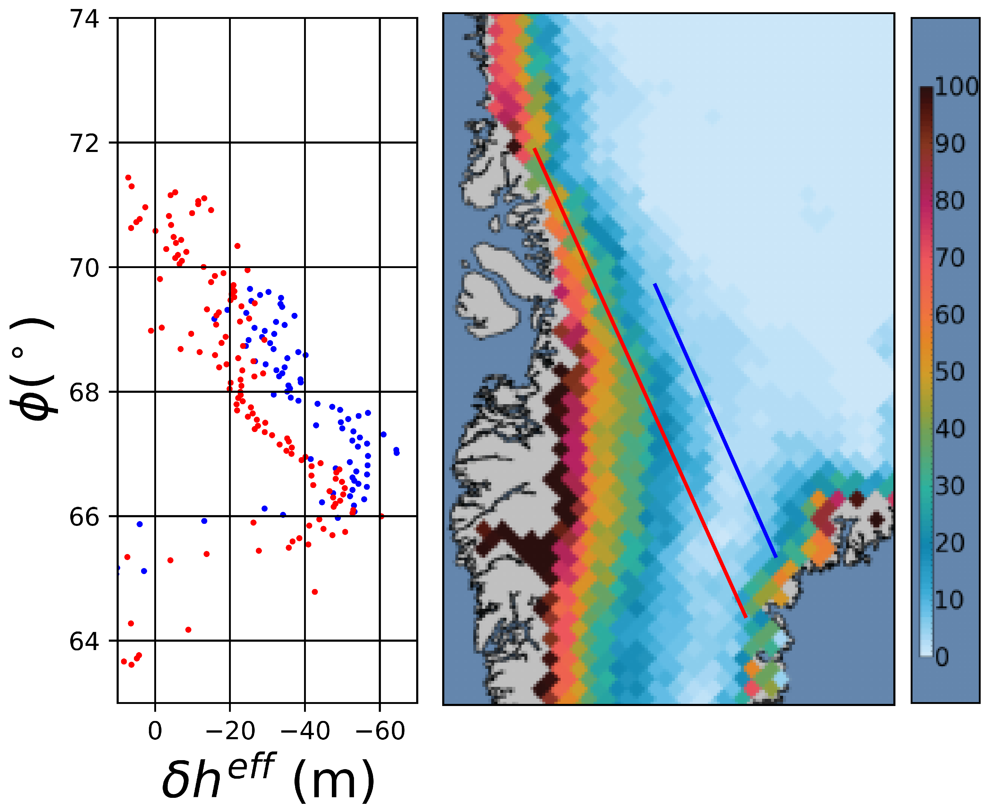
Now we compare qualitatively the results with the melting extent of the Greenland ice sheet, measured with passive microwave instruments [48]. This is done in Figure 9, where it is shown in parallel with a map of the NSIDC Greenland Cumulative Melt Days (GCM). The retrieved effective heights appears correlated with the number of melting days, which in turn correspond to lighter and drier snow conditions. As mentioned above, percolation zones such as the northern tip of the track observed in 27 January (red color) present denser ice profiles, which are less prompt to penetration. Consequently, the efficient height is closer to the surface elevation provided by ICESat (smaller ). These measurements might therefore be a potential contributor to characterize the upper layers of the ice, as variations in homogeneity, density and liquid water content change the penetration capabilities of the signal.
The comparison is also affected by the dispersion of the data (of the order of 10 m in 1 s sampling), and probably biased by residual effects. One of the residual effects is related with the instrumentation used: the TDS-1 GNSS-R receiver has very low delay resolution (≈75 m, on the order of ), and this coarse sampling may introduce biases which in turn can be different over the sea (broader shaped waveforms) from those biases over the ice (narrower shaped waveforms, see the differences in in Figure 4). Therefore, the calibration strategy presented in Section 4, with corrections estimated from the tracks segments over the sea, might not fully correct the potential biases over ice. Instrumentation capturing wider band signals with higher gain antennas, lower noise receivers and correlators with higher resolution, as planned for GEROS-ISS mission [14] payload, should help in reducing these uncertainties. Future analysis should also benefit from the more extensive ground truth information, such as, e.g., data along the EGIG transect (e.g., [49]) or the outcome of NASA IceBridge campaigns (e.g., [50,51]). Furthermore, analysis of the presence of sea ice at the coast of Greenland could also be studied, as suggested in [27,29,30,31,32].
6. Conclusions
This work presents, for the first time, a feasibility study of ice-sheet altimetry, using L-Band GNSS signals. We have used Delay Doppler Maps (DDM) gathered by the TDS-1 mission overflying the southern part of Greenland, in two consecutive days.
The information contained in the DDMs have been inverted to obtain altimetric estimates, and the retrieved height shows, as expected, significant discrepancy with the the ice surface elevation corresponding to the topography given by NSIDC GLAS/ICESat. The difference between the GNSS-R derived surface height and the ice surface elevation can be related to the penetration of the L-band signal into the ice-sheet, which is in the range of [0–60] m, compatible with those obtained in monostatic L-Band radar missions.
This feasibility study shows that a future cryospheric GNSS-R space mission, working with L1, L2 and L5, could provide simultaneous measurements corresponding to different penetration depths of an ice sheet. Such measurements will complement data obtained with other technologies working at different bands.
Acknowledgments
This work has been carried out with the financial support of the Spanish research project ESP2015-70014-C2-2-R (MINECO/FEDER). The authors are grateful to Surrey Satellite Technology Ltd. for making the TDS-1 GNSS-R DDM data available trough the MERRByS website (http://www.merbys.org). We would like to thank the editors and the anonymous reviewers for their help to improve the quality of the paper.
Author Contributions
A.R. coordinated the study. A.R., E.C., F.F., W.L. and S.R. contributed equally to the analysis and interpretation of the GNSS-R aspects of this study. M.H.-P. contributed to the analysis and interpretation of the ionospheric part.
Conflicts of Interest
The authors declare no conflict of interest. The funding sponsors had no role in the design of the study, in the collection, analyses, or interpretation of data, in the writing of the manuscript, and in the decision to publish the results.
Abbreviations
The following abbreviations are used in this manuscript:
| CYGNSS | Cyclone Global Navigation Satellite System |
| DDM | Delay-Doppler Map |
| DEM | Digital Elevation Model |
| EGM | Earth Gravitational Model |
| GCM | Greenland Cumulative Melt |
| GIM | Global Ionospheric Maps |
| GNSS | Global Navigation Satellite System |
| GNSS-R | GNSS Reflectometry |
| cGNSS-R | Conventional GNSS-R |
| iGNSS-R | Interferometric GNSS-R |
| GPS | Global Positioning System |
| IGS | International GNSS Service |
| NEEM | North Greenland Eemian Ice Drilling |
| NSIDC | National Snow and Ice Data Center |
| Signal-to-Noise Ratio | |
| TDS | TechDemoSat |
| TDX | Tandem-X Mission |
| VTEC | Vertical Total Electron Content |
| WGS | World Geodetic System |
References
- Gregory, J.M.; Huybrechts, P.; Raper, S.C.B. Climatology: Threatened loss of the Greenland ice-sheet. Nature 2004, 428, 616. [Google Scholar] [CrossRef] [PubMed] [Green Version]
- Lythe, M.B.; Vaughan, D.G. BEDMAP: A new ice thickness and subglacial topographic model of Antarctica. J. Geophys. Res. Solid Earth 2001, 106, 11335–11351. [Google Scholar] [CrossRef]
- Church, J.A.; Clark, P.U.; Cazenave, A.; Gregory, J.M.; Jevrejeva, S.; Leverman, A.; Merrifield, M.A.; Milne, G.A.; Nerem, R.S.; Nunn, P.D.; et al. Sea Level Change. In Climate Change 2013: The Physical Science Basis. Contribution of Working Group I to the Fifth Assessment Report of the Intergovernmental Panel on Climate Change; Cambridge University Press: Cambridge, UK; New York, NY, USA, 2013. [Google Scholar]
- Mouginot, J.; Rignot, E.; Scheuchl, B.; Fenty, I.; Khazendar, A.; Morlighem, M.; Buzzi, A.; Paden, J. Fast retreat of Zachariæ Isstrøm, northeast Greenland. Science 2015, 350, 1357–1361. [Google Scholar] [CrossRef] [PubMed]
- McMillan, M.; Shepherd, A.; Sundal, A.; Briggs, K.; Muir, A.; Ridout, A.; Hogg, A.; Wingham, D. Increased ice losses from Antarctica detected by CryoSat-2. Geophys. Res. Lett. 2014, 41, 3899–3905. [Google Scholar] [CrossRef]
- Nghiem, S.V.; Hall, D.K.; Mote, T.L.; Tedesco, M.; Albert, M.R.; Keegan, K.; Shuman, C.A.; DiGirolamo, N.E.; Neumann, G. The extreme melt across the Greenland ice sheet in 2012. Geophys. Res. Lett. 2012, 39. [Google Scholar] [CrossRef]
- Zwally, H.J.; Schutz, B.; Abdalati, W.; Abshire, J.; Bentley, C.; Brenner, A.; Bufton, J.; Dezio, J.; Hancock, D.; Harding, D.; et al. ICESat’s laser measurements of polar ice, atmosphere, ocean, and land. J. Geodyn. 2002, 34, 405–445. [Google Scholar] [CrossRef]
- Wingham, D.J.; Francis, C.R.; Baker, S.; Bouzinac, C.; Brockley, D.; Cullen, R.; de Chateau-Thierry, P.; Laxon, S.W.; Mallow, U.; Mavrocordatos, C.; et al. CryoSat: A mission to determine the fluctuations in Earth’s land and marine ice fields. Adv. Space Res. 2006, 37, 841–871. [Google Scholar] [CrossRef]
- Brenner, A.C.; DiMarzio, J.P.; Zwally, H.J. Precision and Accuracy of Satellite Radar and Laser Altimeter Data Over the Continental Ice Sheets. IEEE Trans. Geosci. Remote Sens. 2007, 45, 321–331. [Google Scholar] [CrossRef]
- Martin-Neira, M.; D’Addio, S.; Buck, C.; Floury, N.; Prieto-Cerdeira, R. The PARIS Ocean Altimeter In-Orbit Demonstrator. IEEE Trans. Geosci. Remote Sens. 2011, 49, 2209–2237. [Google Scholar] [CrossRef]
- Ruf, C.; Unwin, M.; Dickinson, J.; Rose, R.; Rose, D.; Vincent, M.; Lyons, A. CYGNSS: Enabling the Future of Hurricane Prediction [Remote Sensing Satellites]. IEEE Geosci. Remote Sens. Mag. 2013, 1, 52–67. [Google Scholar] [CrossRef]
- Cardellach, E.; Rius, A.; Martin-Neira, M.; Fabra, F.; Nogués-Correig, O.; Ribó, S.; Kainulainen, J.; Camps, A.; D’Addio, S. Consolidating the Precision of Interferometric GNSS-R Ocean Altimetry Using Airborne Experimental Data. IEEE Trans. Geosci. Remote Sens. 2014, 52, 4992–5004. [Google Scholar] [CrossRef]
- Camps, A.; Park, H.; Domènech, E.V.i.; Pascual, D.; Martin, F.; Rius, A.; Ribó, S.; Benito, J.; Andrés-Beivide, A.; Saameno, P.; et al. Optimization and Performance Analysis of Interferometric GNSS-R Altimeters: Application to the PARIS IoD Mission. IEEE J. Sel. Top. Appl. Earth Obs. Remote Sens. 2014, 7, 1436–1451. [Google Scholar] [CrossRef]
- Wickert, J.; Cardellach, E.; Martín-Neira, M.; Bandeiras, J.; Bertino, L.; Andersen, O.B.; Camps, A.; Catarino, N.; Chapron, B.; Fabra, F.; et al. GEROS-ISS: GNSS REflectometry, Radio Occultation, and Scatterometry Onboard the International Space Station. IEEE J. Sel. Top. Appl. Earth Obs. Remote Sens. 2016, 9, 4552–4581. [Google Scholar] [CrossRef]
- Unwin, M.; Jales, P.; Tye, J.; Gommenginger, C.; Foti, G.; Rosello, J. Spaceborne GNSS-Reflectometry on TechDemoSat-1: Early Mission Operations and Exploitation. IEEE J. Sel. Top. Appl. Earth Obs. Remote Sens. 2016, 9, 4525–4539. [Google Scholar] [CrossRef]
- Cardellach, E.; Ao, C.O.; de la Torre Juárez, M.; Hajj, G.A. Carrier phase delay altimetry with GPS-reflection/occultation interferometry from low Earth orbiters. Geophys. Res. Lett. 2004, 31, 377–393. [Google Scholar] [CrossRef]
- Cardellach, E.; Fabra, F.; Rius, A.; Pettinato, S.; D’Addio, S. Characterization of dry-snow sub-structure using GNSS reflected signals. Remote Sens. Environ. 2012, 124, 122–134. [Google Scholar] [CrossRef]
- Pavlis, N.K.; Holmes, S.A.; Kenyon, S.C.; Factor, J.K. The development and evaluation of the Earth Gravitational Model 2008 (EGM2008). J. Geophys. Res. Solid Earth 2012, 117, B04406. [Google Scholar] [CrossRef]
- Benson, C. Stratigraphic Studies in the Snow and Firn of the Greenland Ice Sheet; Cold Regions Research and Engineering Lab: Hanover, NH, USA, 1962. [Google Scholar]
- Jales, P.; Unwin, M. MERRByS Product Manual: GNSS-Reflectometry on TDS-1 with the SGR-ReSI; Surrey Satellite Technol. Ltd.: Guildford, UK, 2015. [Google Scholar]
- Jales, P. Spaceborne Receiver Design for Scatterometric GNSS Reflectometr. Ph.D. Thesis, University of Surrey, Guildford, UK, 2012. [Google Scholar]
- Schiavulli, D.; Nunziata, F.; Migliaccio, M.; Frappart, F.; Ramilien, G.; Darrozes, J. Reconstruction of the Radar Image From Actual DDMs Collected by TechDemoSat-1 GNSS-R Mission. IEEE J. Sel. Top. Appl. Earth Obs. Remote Sens. 2016, 9, 4700–4708. [Google Scholar] [CrossRef]
- Foti, G.; Gommenginger, C.; Jales, P.; Unwin, M.; Shaw, A.; Robertson, C.; Roselló, J. Spaceborne GNSS reflectometry for ocean winds: First results from the UK TechDemoSat-1 mission. Geophys. Res. Lett. 2015, 42, 5435–5441. [Google Scholar] [CrossRef] [Green Version]
- Camps, A.; Park, H.; Pablos, M.; Foti, G.; Gommenginger, C.; Liu, P.W.; Judge, J. Soil moisture and vegetation impact in GNSS-R TechDemosat-1 observations. In Proceedings of the 2016 IEEE International Geoscience and Remote Sensing Symposium (IGARSS), Beijing, China, 10–15 July 2016; pp. 1982–1984. [Google Scholar]
- Chew, C.; Shah, R.; Zuffada, C.; Hajj, G.; Masters, D.; Mannucci, A.J. Demonstrating soil moisture remote sensing with observations from the UK TechDemoSat-1 satellite mission. Geophys. Res. Lett. 2016, 43, 3317–3324. [Google Scholar] [CrossRef]
- Camps, A.; Park, H.; Foti, G.; Gommenginger, C. Ionospheric Effects in GNSS-Reflectometry From Space. IEEE J. Sel. Top. Appl. Earth Obs. Remote Sens. 2016, 9, 5851–5861. [Google Scholar] [CrossRef]
- Hu, C.; Benson, C.; Rizos, C.; Qiao, L. Single-Pass Sub-Meter Space-Based GNSS-R Ice Altimetry: Results From TDS-1. IEEE J. Sel. Top. Appl. Earth Obs. Remote Sens. 2017, 1–7. [Google Scholar] [CrossRef]
- Clarizia, M.P.; Ruf, C.; Cipollini, P.; Zuffada, C. First spaceborne observation of sea surface height using GPS-Reflectometry. Geophys. Res. Lett. 2016, 43, 767–774. [Google Scholar] [CrossRef] [Green Version]
- Yan, Q.; Huang, W. Spaceborne GNSS-R Sea Ice Detection Using Delay-Doppler Maps: First Results From the U.K. TechDemoSat-1 Mission. IEEE J. Sel. Top. Appl. Earth Obs. Remote Sens. 2016, 9, 4795–4801. [Google Scholar] [CrossRef]
- AlonsoArroyo, A.; Zavorotny, V.U.; Camps, A. Sea ice detection using GNSS-R data from UK TDS-1. In Proceedings of the 2016 IEEE International Geoscience and Remote Sensing Symposium (IGARSS), Beijing, China, 10–15 July 2016; pp. 2001–2004. [Google Scholar]
- Yan, Q.; Huang, W.; Moloney, C. Neural Networks Based Sea Ice Detection and Concentration Retrieval From GNSS-R Delay-Doppler Maps. IEEE J. Sel. Top. Appl. Earth Obs. Remote Sens. 2017, 1–10. [Google Scholar] [CrossRef]
- Schiavulli, D.; Frappart, F.; Ramillien, G.; Darrozes, J.; Nunziata, F.; Migliaccio, M. Observing Sea/Ice Transition Using Radar Images Generated From TechDemoSat-1 Delay Doppler Maps. IEEE Geosci. Remote Sens. Lett. 2017, 14, 734–738. [Google Scholar] [CrossRef]
- Elachi, C. Spaceborne Radar Remote Sensing: Applications and Techniques; IEEE Press: New York, NY, USA, 1988. [Google Scholar]
- Hajj, G.A.; Zuffada, C. Theoretical description of a bistatic system for ocean altimetry using the GPS signal. Radio Sci. 2003, 38, 1089. [Google Scholar] [CrossRef]
- Rius, A.; Cardellach, E.; Martin-Neira, M. Altimetric Analysis of the Sea-Surface GPS-Reflected Signals. IEEE Trans. Geosci. Remote Sens. 2010, 48, 2119–2127. [Google Scholar] [CrossRef]
- Zavorotny, V.U.; Voronovich, A.G. Scattering of GPS signals from the ocean with wind remote sensing application. IEEE Trans. Geosci. Remote Sens. 2000, 38, 951–964. [Google Scholar] [CrossRef]
- Wiehl, M.; Legresy, B.; Dietrich, R. Potential of reflected GNSS signals for ice sheet remote sensing. Prog. Electromagn. Res. 2003, 40, 177–205. [Google Scholar] [CrossRef]
- Egbert, G.D.; Erofeeva, S.Y. Efficient Inverse Modeling of Barotropic Ocean Tides. J. Atmos. Ocean. Technol. 2002, 19, 183–204. [Google Scholar] [CrossRef]
- Misra, P.; Enge, P. Global Positioning System: Signals, Measurements and Performance, 2nd ed.; Ganga-Jamuna Press: Lincoln, MA, USA, 2006. [Google Scholar]
- Hernández Pajares, M.; Roma Dollase, D.; Krankowski, A.; García Rigo, A.; Orús Pérez, R. Comparing performances of seven different global VTEC ionospheric models in the IGS context. In Proceedings of the International GNSS Service Workshop (IGS 2016), Sydney, Australia, 8–12 February 2016; pp. 1–13. [Google Scholar]
- Gleason, S.; Hodgart, S.; Sun, Y.; Gommenginger, C.; Mackin, S.; Adjrad, M.; Unwin, M. Detection and Processing of bistatically reflected GPS signals from low Earth orbit for the purpose of ocean remote sensing. IEEE Trans. Geosci. Remote Sens. 2005, 43, 1229–1241. [Google Scholar] [CrossRef]
- Bracewell, R. The Fourier Transform and Its Applications; Electrical and Electronic Engineering; McGraw-Hill: New York, NY, USA, 1965. [Google Scholar]
- Hoen, E.W.; Zebker, H.A. Penetration depths inferred from interferometric volume decorrelation observed over the Greenland ice sheet. IEEE Trans. Geosci. Remote Sens. 2000, 38, 2571–2583. [Google Scholar]
- Ulaby, F.T.; Moore, R.K.; Fung, A.K. Volume 2—Radar remote sensing and surface scattering and emission theory. In Microwave Remote Sensing: Active and Passive; Artech House: Norwood, MA, USA, 1982. [Google Scholar]
- Fujita, S.; Hirabayashi, M.; Goto-Azuma, K.; Dallmayr, R.; Satow, K.; Zheng, J.; Dahl-Jensen, D. Densification of layered firn of the ice sheet at NEEM, Greenland. J. Glaciol. 2014, 60, 905–921. [Google Scholar] [CrossRef]
- Simonsen, S.B.; Stenseng, L.; Aðalgeirsdóttir, G.; Fausto, R.S.; Hvidberg, C.S.; Lucas-Pichery, P. Assessing a multilayered dynamic firn-compaction model for Greenland with ASIRAS radar measurements. J. Glaciol. 2013, 59, 545–558. [Google Scholar] [CrossRef]
- Rignot, E.; Echelmeyer, K.; Krabill, W. Penetration depth of interferometric synthetic-aperture radar signals in snow and ice. Geophys. Res. Lett. 2001, 28, 3501–3504. [Google Scholar] [CrossRef]
- Mote, T.L.; Anderson, M.R. Variations in snowpack melt on the Greenland ice sheet based on passive-microwave measurements. J. Glaciol. 1995, 41, 51–60. [Google Scholar] [CrossRef]
- Overly, T.B.; Hawley, R.L.; Helm, V.; Morris, E.M.; Chaudhary, R.N. Greenland annual accumulation along the EGIG line, 1959–2004, from ASIRAS airborne radar and neutron-probe density measurements. Cryosphere 2016, 10, 1679–1694. [Google Scholar] [CrossRef]
- Forster, R.R.; van den Broeke, M.R.; Miège, C.; Burgess, E.W.; van Angelen, J.H.; Lenaerts, J.T.; Koenig, L.S.; Paden, J.; Lewis, C.; Gogineni, S.P.; et al. Extensive liquid meltwater storage in firn within the Greenland ice sheet. Nat. Geosci. 2014, 7, 95–98. [Google Scholar] [CrossRef]
- Koenig, L.S.; Alexander, P.M.; MacGregor, J.A.; Paden, J.D.; Forster, R.R.; McConnell, J.R. Annual Greenland accumulation rates (2009–2012) from airborne snow radar. Cryosphere 2016, 10, 1739. [Google Scholar] [CrossRef]
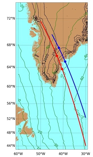
Figure 1.
Map of the region considered in this study, containing the southern part of Greenland. The black contour levels over Greenland have been extracted from the National Snow and Ice Data Center (NSIDC) GLAS/ICESat 1 km laser altimetry digital elevation model of Greenland [9]. The green contour lines have been obtained from the Earth Gravitational Model (EGM) 2008 [18]. The two transects correspond to the specular points selected in this study, crossing different Benson facies [19]. The blue trace corresponds to 26 January 2015, and the red one to the day after. There are two points that divide, from South to North, each trace in three sections, sea, topographic step, and ice, with different prevailing scattering mechanisms. Within these tracks the peak-to-peak variations of the heights with respect WGS84 are on the order of ten meters for the WGM2008 levels, while they are of two kilometers for the (NSIDC) GLAS/ICESat levels.
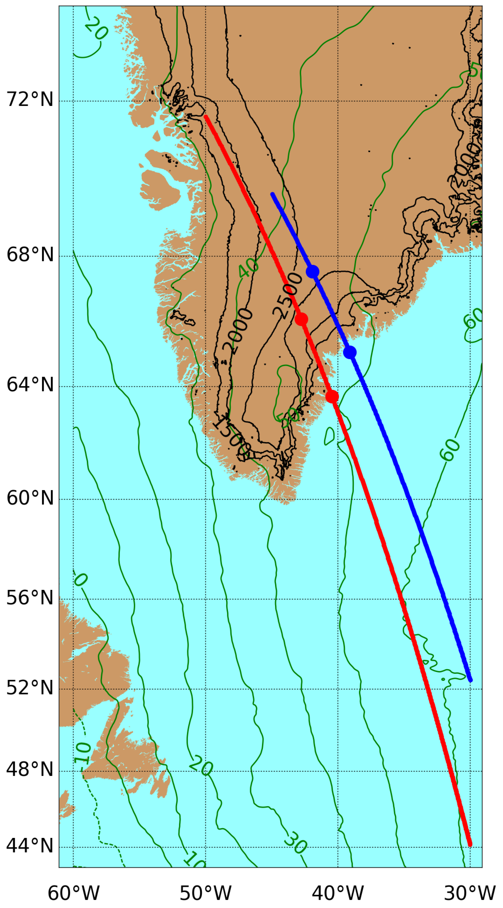
Figure 2.
The normalized power of a simulated TDS-1 one-second sea DDM, computed with typical values encountered in the TDS-1 situation. The origin of the coordinate system has been assigned to the point corresponding to the observed delay and . The TDS-1 resolution is indicated by the small red box. The larger red rectangle indicates the TDS-1 correlation pixels used in this altimetric study. The beginning and end of the waveform are indicated with the labels and . The point corresponds to the TDS-1 a priori reference and is the corresponding a priori value considered in this study.

Figure 3.
The modeled delays due to tidal (green), ionospheric (blue) and tropospheric effects (red), are represented for the two transects. (a) 26 January 2015. (b) 27 January 2015.
Figure 3.
The modeled delays due to tidal (green), ionospheric (blue) and tropospheric effects (red), are represented for the two transects. (a) 26 January 2015. (b) 27 January 2015.
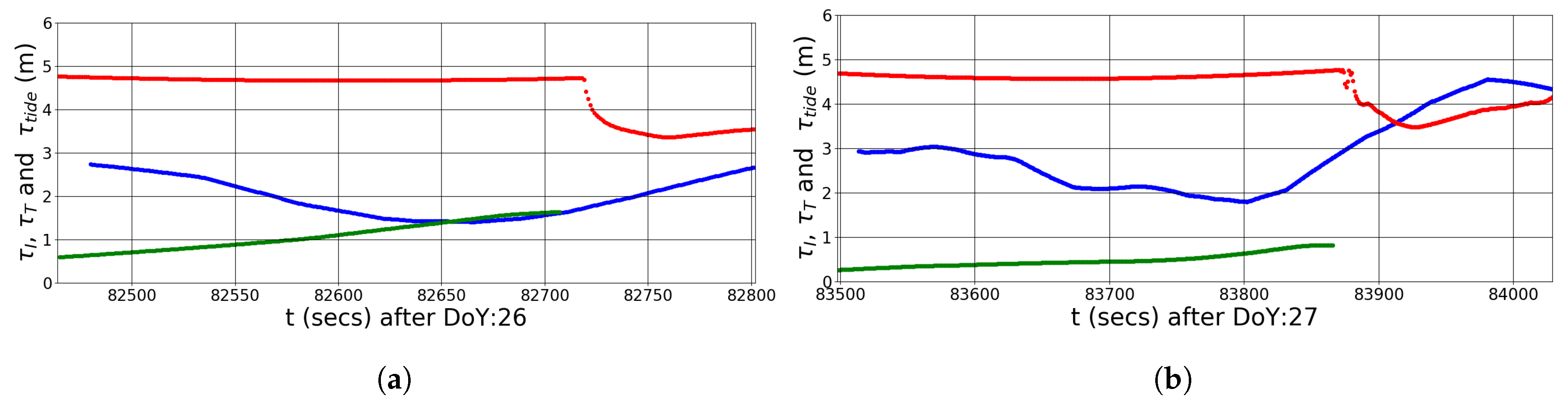
Figure 4.
Two panels showing the time evolution of the power waveforms, one for each track. The left-hand figure in each panel contains the waveform widths , defined at their 3-dB level. The vertical red line corresponds to the width of unscattered GPS C/A code signals. In the middle figure of each panel we show the modeled delay as expected with respect to a reflection off a point on the reference WGS-84 ellipsoid. The model has assumed surface topographies provided by the EGM 2008 geoid over the sea and by NSIDC GLAS/ICESat over Greenland. In the right figure of each panel we present all the waveforms 2D image. (a) 26 January 2015. (b) 27 January 2015.
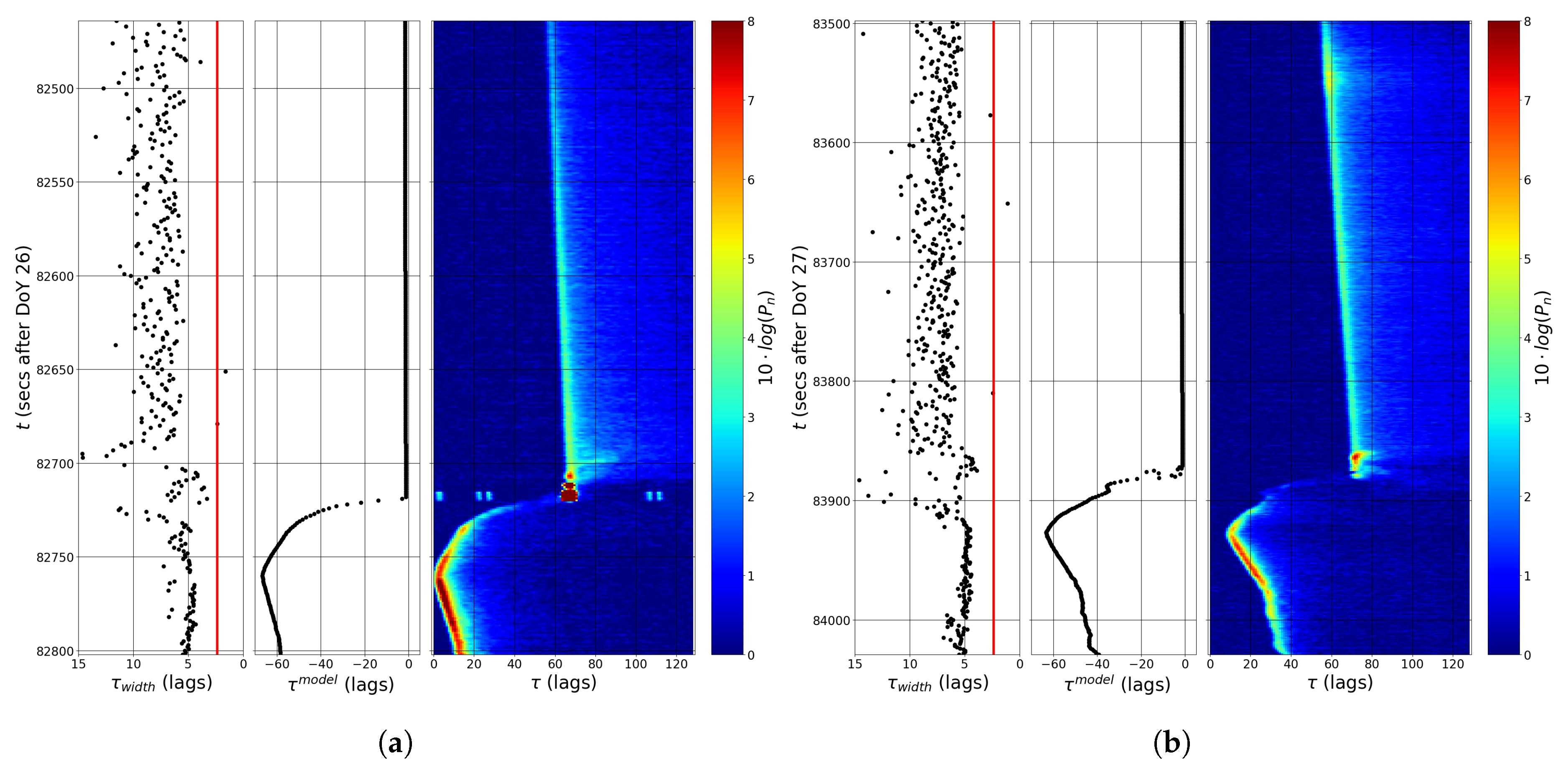
Figure 5.
The observed delays and their standard deviation obtained from the sea waveforms. Superimposed on the values we include a running mean used to derive . The trend in the observed delays is attributed in this study to effects of TDS-1 clock inaccuracies. (a) 26 January 2015. (b) 27 January 2015.

Figure 6.
The differential delays and their standard deviation obtained from the whole data set, after correcting for the trend derived from the sea waveforms. Superimposed to the values we include a running mean used to derive . (a) 26 January 2015. (b) 27 January 2015.
Figure 6.
The differential delays and their standard deviation obtained from the whole data set, after correcting for the trend derived from the sea waveforms. Superimposed to the values we include a running mean used to derive . (a) 26 January 2015. (b) 27 January 2015.

Figure 7.
In each column we have represented from bottom to top (1) the topography associated to each track , (2) the estimate of the apparent the height relative to the a priori model , and (3) its standard deviation . (a) 26 January 2015. (b) 27 January 2015.
Figure 7.
In each column we have represented from bottom to top (1) the topography associated to each track , (2) the estimate of the apparent the height relative to the a priori model , and (3) its standard deviation . (a) 26 January 2015. (b) 27 January 2015.

Figure 8.
Refractive index as a function of ice depth, as reported in Table 4 of Ref [45], estimated from North Greenland Eemian Ice Drilling (NEEM) camp data.
Figure 8.
Refractive index as a function of ice depth, as reported in Table 4 of Ref [45], estimated from North Greenland Eemian Ice Drilling (NEEM) camp data.

Figure 9.
(a) Estimates of as a function of the latitude of the specular point for the 26 January 2015 track (blue), and the 27 January 2015 (red). (b) Section of the Greenland Map, courtesy of University of Georgia/Thomas Mote, supplied by the National Snow and Ice Data Center, University of Colorado, showing the number of melting days [48], indicated by the color scale, for the period January–October 2016. The two traces correspond to the approximate location of the specular points considered.


Table 1.
Selected TDS-1 Data waveforms.
| First Transect | Second Transect | |
|---|---|---|
| TDS-1 RD ID | 16 | 16 |
| TDS-1 Track ID | 120 | 765 |
| Date | 26 January 2015 | 27 January 2015 |
| Second of Day | 82,470–82,800 (s) | 83,505–84,200 (s) |
| GPS PRN | 31 | 31 |
| SP Lat&Lon (Start) | [52.775N, 30.164W] | [43.687N, 25.605W] |
| SP Lat&Lon (End) | [69.574N, 44.747W] | [78.828N, 71.880W] |
| Incidence angle i | 3–19 () | 4–28 () |
| Gain | 8–12 (dBi) | 8–13 (dBi) |
© 2017 by the authors. Licensee MDPI, Basel, Switzerland. This article is an open access article distributed under the terms and conditions of the Creative Commons Attribution (CC BY) license (http://creativecommons.org/licenses/by/4.0/).
Share and Cite
MDPI and ACS Style
Rius, A.; Cardellach, E.; Fabra, F.; Li, W.; Ribó, S.; Hernández-Pajares, M. Feasibility of GNSS-R Ice Sheet Altimetry in Greenland Using TDS-1. Remote Sens. 2017, 9, 742. https://doi.org/10.3390/rs9070742
AMA Style
Rius A, Cardellach E, Fabra F, Li W, Ribó S, Hernández-Pajares M. Feasibility of GNSS-R Ice Sheet Altimetry in Greenland Using TDS-1. Remote Sensing. 2017; 9(7):742. https://doi.org/10.3390/rs9070742
Chicago/Turabian StyleRius, Antonio, Estel Cardellach, Fran Fabra, Weiqiang Li, Serni Ribó, and Manuel Hernández-Pajares. 2017. "Feasibility of GNSS-R Ice Sheet Altimetry in Greenland Using TDS-1" Remote Sensing 9, no. 7: 742. https://doi.org/10.3390/rs9070742
Note that from the first issue of 2016, this journal uses article numbers instead of page numbers. See further details here.