
Pre-Flight SAOCOM-1A SAR Performance Assessment by Outdoor Campaign


1
ARESYS srl, Via Flumendosa 16, 20132 Milan, Italy
2
Politecnico di Milano, Piazza Leonardo da Vinci 32, 20133 Milan, Italy
3
CONAE, Avda. Paseo Colon 751, 1063 Buenos Aires, Argentina
*
Author to whom correspondence should be addressed.
Remote Sens. 2017, 9(7), 729; https://doi.org/10.3390/rs9070729
Submission received: 23 May 2017
/
Revised: 7 July 2017
/
Accepted: 12 July 2017
/
Published: 14 July 2017
(This article belongs to the Special Issue Advances in SAR: Sensors, Methodologies, and Applications)
Abstract
:In the present paper, we describe the design, execution, and the results of an outdoor experimental campaign involving the Engineering Model of the first of the two Argentinean L-band Synthetic Aperture Radars (SARs) of the Satélite Argentino de Observación con Microondas (SAOCOM) mission, SAOCOM-1A. The experiment’s main objectives were to test the end-to-end SAR operation and to assess the instrument amplitude and phase stability as well as the far-field antenna pattern, through the illumination of a moving target placed several kilometers away from the SAR. The campaign was carried out in Bariloche, Argentina, during June 2016. The experiment was successful, demonstrating an end-to-end readiness of the SAOCOM-SAR functionality in realistic conditions. The results showed an excellent SAR signal quality in terms of amplitude and phase stability.
1. Introduction
The forthcoming Argentinean mission Satélite Argentino de Observación con Microondas (SAOCOM) [1] is constituted by two identical Low-Earth-Orbit (LEO) satellites, SAOCOM-1A and -1B, carrying as the main payload an L-band Synthetic Aperture Radar (SAR). The SAOCOM-SAR has an active array antenna with elevation and azimuth steering capability for frequent-revisit, wide-swath, and medium resolution Earth observation.
The mission’s target applications [2] require a tight overall amplitude and phase stability performance, which is imposed to a large extent by the instrument critical elements, such as the chirp generator, the distribution network, the Transmit-Receive Modules (TRMs), the clock, and the antenna. The pre-launch assessment and verification of the phase and amplitude performance is paramount in order to limit the calibration and verification efforts to be done in-flight (e.g., during the commissioning phase).
Typically, the instrument elements can be tested on a singular basis, and the antenna far-field radiation pattern can be reconstructed from planar-near-field-scanner (PNFS) measurements of the near field radiation patterns of the elements of the antenna by means of an accurate antenna model [3]. In the latter case, extreme care is needed in the measurement setup to avoid biases in the measurements. The far-field pattern is not available on-ground and the antenna model can be verified only in-flight, exploiting e.g., homogeneous targets for the elevation case and recording transponders for the azimuth. A typical example is the acquisition over the Amazonian rainforest. However, the in-flight data intensity profile depends on a list of other factors (e.g., pointing, time-variant instrument gains, processor gains), also to be calibrated or verified, so that it might be difficult to isolate the antenna contribution from the others, as reported for the case of Sentinel-1 in References [4,5]. Furthermore, the in-flight verification allows a limited verification of the elevation antenna pattern, within the angular range used by the imaging swath.
One way to check the mid- and long-term stability of the system, say from seconds to minutes, is an outdoor experiment where SAR acquisitions are carried out with the full antenna (or a part of it, e.g., one tile) pointed to targets of opportunity or man-made calibrators in the far-field. In addition, the collected power measures for different antenna pointing can be correlated to the theoretical antenna model to obtain a first far-field verification, complementary to what could be obtained with PNFS measurements.
2. Outdoor Experiment Concept, Design, and Simulations
The well-known far field condition on the distance R for an antenna with size L operating at central wavelength λ, is:
In the case of the SAOCOM-1A SAR instrument, we refer to the SAR antenna, a planar array with the total size along azimuth L equal to 9.94 m. The antenna is made by seven tiles with the size of 1.42 m × 3.48 m (azimuth × elevation), and the center frequency is 1.275 GHz ( is equal to 23.53 cm). The far field distance results are in the order of 40 m. Moreover, the SAR instrument cannot receive echoes returning to the antenna while the chirp transmission is still active. Considering a minimum chirp length of 10 μs, and another 10 μs of guard time between the end of transmission and the start of echo reception, the minimum distance of a “visible” target is 3.3 km.
Compared to the SAR acquisition in space, here the antenna is not moving along an orbit, so there is no synthetic aperture. The area illuminated by the antenna is limited by the range resolution and by the real antenna aperture in azimuth . Considering a homogeneous reflective scenario (e.g., bare soil or short vegetation) in front of the radar, with reflectivity equal to , the radar cross-section (RCS) of each resolution cell is computed as:
Considering the bandwidth range equal to 50 MHz and one tile of the antenna with a length equal to 1.42 m, the resolution cell at the SAOCOM central frequency is as large as 1600 m2. Assuming a reflectivity of −15 dB, the obtained RCS is 17 dBsm. (We indicate with dBsm the ratio of the area with respect to 1 m2, expressed in logarithmic scale).
This large backscattered power can be considered either as a signal—if stable—or as a noise—if unstable. Water and leaves are highly unstable; however, their contribution is effectively reduced if averaged for seconds. Slower-moving targets could provide long-term noise contributions that affect the measure. We then decided that the observed scenario might not be stable enough for an accurate measurement, so we inserted a trihedral corner reflector in the scene.
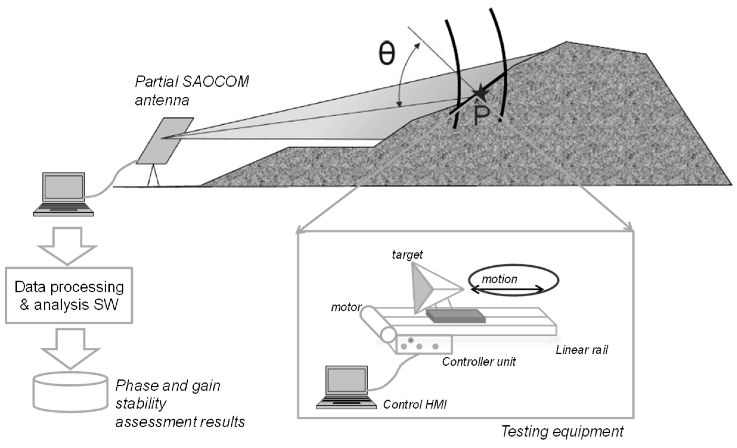
Figure 1 shows the schematic representation of the overall concept of the SAOCOM outdoor test (ODT): the SAOCOM SAR antenna points towards a known point target (trihedral corner reflector), moving along the line of sight, with a linear motion, thanks to a linear actuator. The acquired data are downloaded and processed to extract signal characteristics and to assess the phase and gain stability of the instrument.
The reason for target motion is to effectively limit the size of the corner reflector to reasonable values. The target, moving with controlled and known motion, can be separated from the background and other moving targets provided that the motion is significant with respect to half the wavelength.
The RCS of the trihedral corner reflector with length d can be modeled as:
In order to distinguish it from the background and to have sufficient accuracy in the phase and amplitude measurement, we ask for a signal to clutter ratio of at least 30 dB. With the computed RCS of the clutter as above, this would lead to a target with a size greater than 8 m.
Let us then assume that the corner reflector is mounted on a rail, and moves with time, say of an extent much less than a range resolution cell. The return from successive echoes measured at the target range can be modeled as a mono-dimensional time-variant signal, given by the superposition of the distributed target (or clutter), the signal from the trihedral target, and the noise w, due to thermal and quantization:
where the first integral is extended to the unfocused azimuth aperture, the resolution . In the equation above, τ represents the time and ξ the spatial coordinate. The phase noise term accounts for the propagation within the troposphere and it is discussed later on in the text. The two terms and are the returns, respectively, from the distributed target and the trihedral. The second term is the signal related to the target. The phase term accounts for the motion of the target and represents an equivalent of the “phase history” of the target, to be compensated for (“focused”).
In the case of linear motion along the line of sight with velocity , the phase history corresponds to a linear phase ramp:
And hence the observed data sequence at the target range is a sampled sinusoid with frequency:
The term is the Doppler Frequency created by the target motion. Unlike a spaceborne SAR, in which every target in the scene has its own Doppler, here all the fixed targets appear at Doppler zero except for the one of interest.
Assuming a very good knowledge of the phase , the “focused” target response is retrieved by compensation of the phase on the signal , performing what in SAR focusing is called “backprojection”:
In the following, we study the content of , making different hypotheses on the disturbing phase noise and on the clutter statistics.
The impact of propagation (the phase noise term ), accounts for the additional delay introduced by the non-free space propagation within the troposphere. If the monochromatic approximation holds (a small bandwidth compared to the carrier frequency), the phase term is linearly related to the delay, which in turn depends on the integral of the refraction index along the path.
where N is the space- and time-variant refractivity index of the atmosphere, a function of the space r and the time of acquisition. The statistics of the atmosphere have been widely studied in the past [6]. Limiting the temporal scope to one day (far longer than one SAR acquisition), we can well consider the Kolmogorov turbulence statistical model of the delay, represented by the power law:
where is a temporal constant depending on the local atmospheric conditions (typical values are in the order of hours). The exponent α is also defined as slope, as the function is a line in a log-log space, assuming values experimentally determined to be close to 2/3. The applicability of the model was verified with experimental ground-based radar measurements in Reference [6]. Numerical simulations were carried out to investigate the impact on the obtained signal-to-clutter ratio due to the atmospheric delay spatial and temporal variation.
We now analyze the clutter contribution (the first term in Equation (4)), assuming sufficient stability of the atmosphere in the time interval of one acquisition. This assumption was verified by analyzing the Doppler spectrum of the acquired clutter echoes (see Section 4). The result of the focusing operation in (7) is a stochastic process with variance depending on the clutter spatial and temporal covariance matrix. This will depend on the scenario (e.g., rocks or vegetation) and on its stability (e.g., due to wind).
To show the principle of the outdoor test, we analytically derive the case of clutter perfectly correlated in time (frozen scene). In this case, the clutter is a constant along time, so its contribution to the focused signal is given by:
where L is the total length of the target motion. The relation above shows that the contribution of the clutter to the focused moving target is a cardinal sinc, which depends only on the total motion extent L. With a motion extent multiple of , the clutter power is (ideally) completely cancelled, as the total signal-to-noise ratio is only thermal-noise limited. In this ideal case, the velocity of the target is completely irrelevant (provided that the radar Pulse repetition Frequency (PRF) is sufficient to sample the sinusoid at , which, for typical PRFs in the order of KHz, is practically always true).
3. SAOCOM Outdoor Experiment Setup
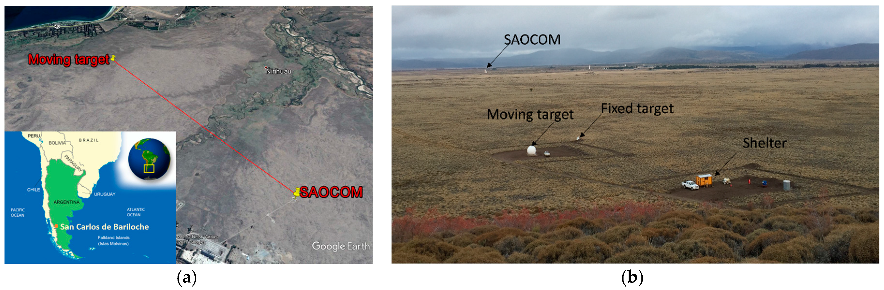
The SAOCOM-1A outdoor test (ODT) took place in the Investigación Aplicada (INVAP) facility close to the Bariloche Airport, Patagonia, Argentina. The facility consisted of a radome hosting one tile of the SAOCOM antenna and the SAOCOM electronics, connected to a control and data-processing room.
The moving target was hosted in a radome placed at a distance of 3755 m in the plane in front of the facility.
Figure 2 shows the setup on Google Earth (a) and an aerial view of the area (b). The picture was taken standing on a small hill of approximately 50 m altitude above the large plane. In the foreground, there is the area hosting the shelter with the guard and the power generator, connected to the small radome hosting the moving target. The fixed target was placed on the right, approximately 20 m away from the radome. Far beyond, the facility hosting the SAOCOM with the large radome can be seen.
Three trihedral corner reflectors were available during the ODT campaign:
- 75 cm
- 100 cm (visible in Figure 3b)
- 150 cm
The first two corner reflectors could be mounted on the moving actuator, while the large one was placed to be kept immobile at approximately 20 m from the moving target radome.
The Advanced Remote Sensing Systems (ARESYS) corners are trihedral-shaped aluminum reflectors with modular faces that were assembled on-site.
Table 1 below reports the RCS in dB square meters (dBsm) of the corner reflectors at the SAOCOM center wavelength (0.2353 m).
The accurate pointing of the corner reflectors mounted on the moving rail was ensured by the alignment of the rail itself with the line of sight, which was carried out by Comisión Nacional de Actividades Espaciales (CONAE) with the use of a differential Global Positioning System (GPS).
The pointing of the large corner reflector was instead performed with the use of a compass and an inclinometer (resulting thus in a coarser pointing). This method was employed because the large corner reflector was thought to have sufficient RCS so as to be left movable around the scene, in order to ease the execution of preliminary visibility tests.
The SAOCOM antenna was one single tile of the total antenna. One tile is composed of 20 elements in the elevation direction and one element in the azimuth direction, with a total size of 3.48 m in elevation and 1.424 m in azimuth. Each TRM was transmitting 50 W with an efficiency of 75%. The excitation coefficients were set according to a Taylor (amplitude only) tapering, in order to shape the side-lobes. The pointing in elevation and azimuth was possible thanks to the mechanical support equipment which could be steered with steps of approximately 1 degree and the knowledge of the pointing was of approximately 0.1 degree. The link budget, accounting for all the gains and losses from the transmitter, through the medium, and to the receiver, and the corresponding signal-to-noise-ratio (SNR) computation, are reported in Table 2 below. The noise figure NF term is used to define the equivalent noise temperature of the receiver and to then compute the thermal noise power with the classical equation:
where KB is the Boltzmann constant, B is the signal bandwidth, and Ta is the ambient temperature (290 K).
The acquisition parameters were set in order to ease the execution of the outdoor test by putting:
- a short chirp to allow close range
- the maximum bandwidth to reduce the resolution
- a reduced sampling window length to avoid unnecessarily large datasets
The main SAOCOM settings are described in Table 3 below.
In addition to the moving target, a sampling equipment was placed to measure the transmitted chirp and to check the PRF.
4. SAOCOM Outdoor Experiment Results
The raw data, provided by a dedicated implementation of the CONAE User Segment Service (CUSS), called mini-CUSS, were non-Block-Adaptive-Quantizer (BAQ) compressed and modulated (at 30 MHz) data. The processing software had then to perform the following steps:
- digital down conversion
- range compression
- azimuth compression
The digital down conversion step performs the demodulation of the signal to baseband. In the employed software, it also allowed the sub-sampling of the input dataset in order to speed up the processing for a fast analysis of the input data. In fact, the PRF of the SAOCOM is quite high compared to the Doppler content of the illuminated scene. The real input samples are also converted into complex samples during this step.
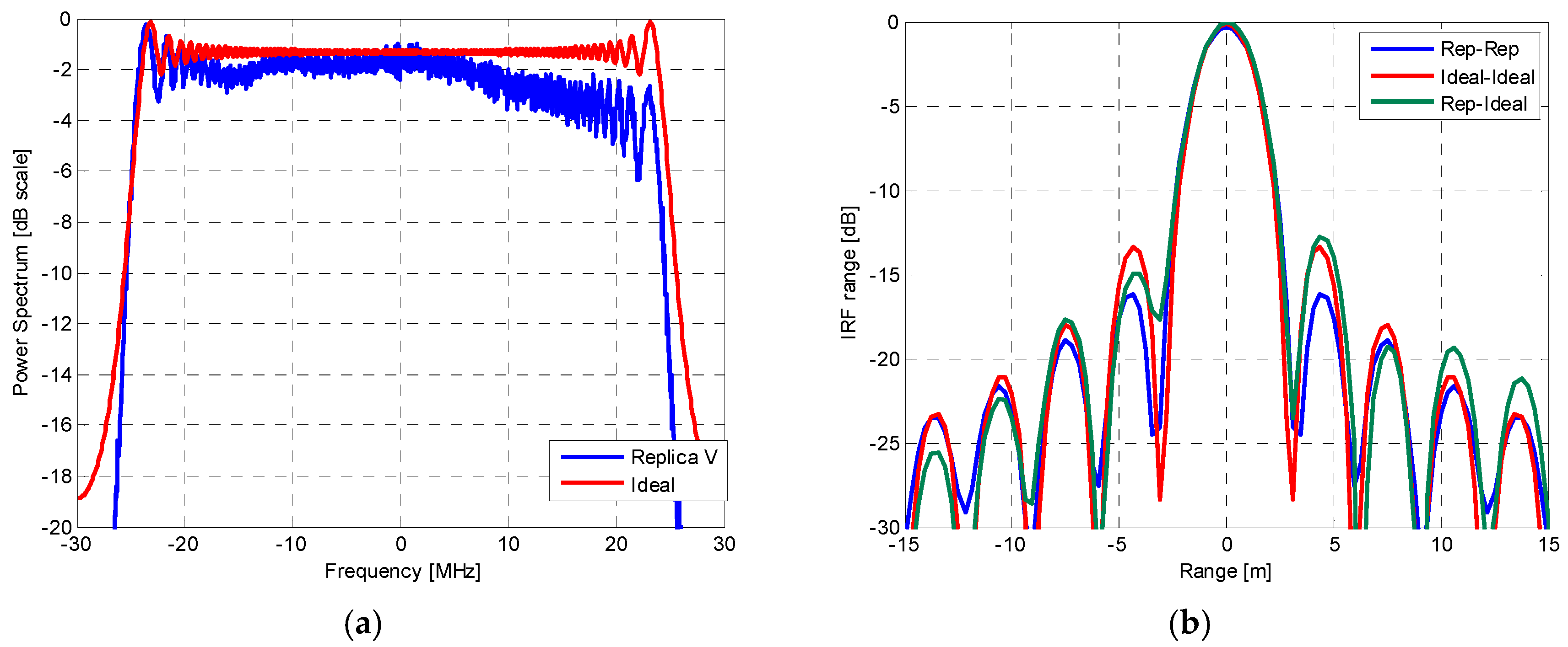
The range compression performs the matched filter either with an ideal chirp (synthetically generated by the routine itself, or with the chirp replica coming from internal calibration.
It is noted that the chirp replica is close to the ideal chirp, except for an amplitude tapering in the upper part of the chirp (Figure 4a). The effect of the imperfect flatness in frequency is seen in the impulse-response-function (IRF) side-lobes level, which are lower than the ideal level of the perfectly rectangular spectrum of the ideal chirp (Figure 4b). The effect on resolution is of about 4% resolution loss (see Table 4), which is almost completely recovered when the replica is focused with the ideal chirp.
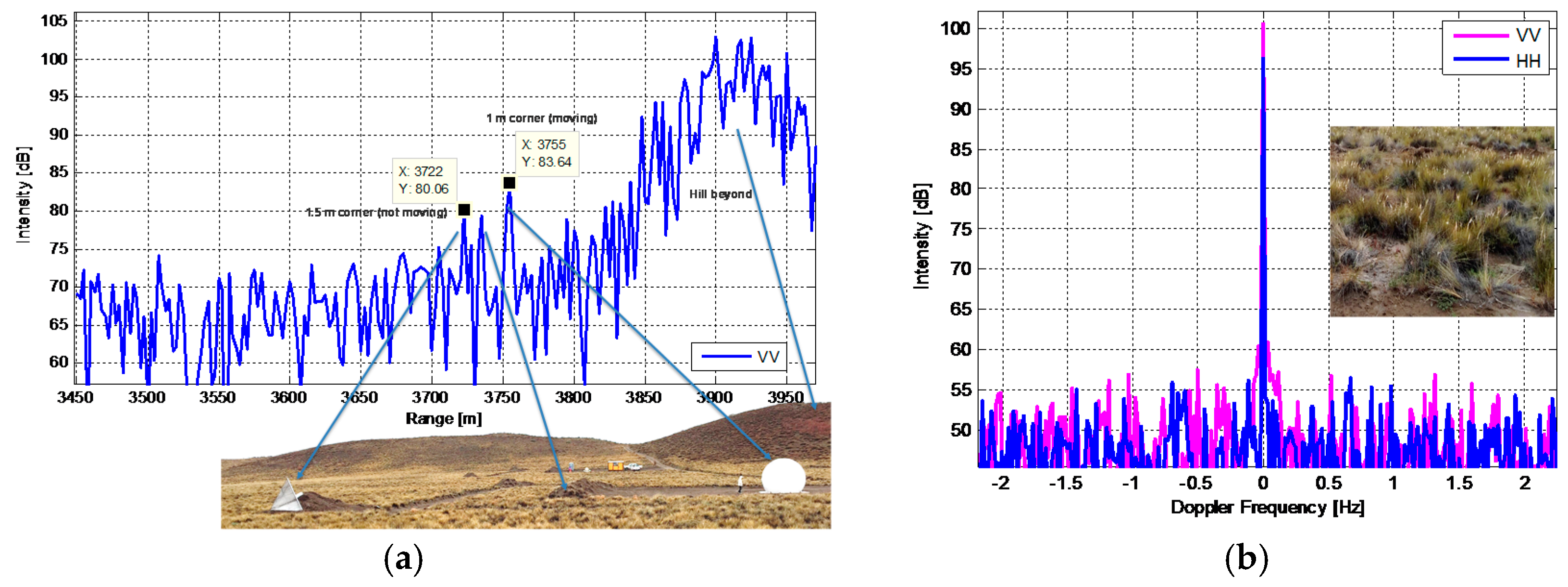
The range power profile of one acquisition is shown in the following figure, for the VV polarization.
The high backscatter from the small hill and three main peaks can be recognized, corresponding to the fixed corner reflector (closest), a small heap of dirt (mid), and the moving target inside the radome (at 3755 m).
The signal to clutter ratio of the latter is approximately 13 dB. Considering the 100-cm corner RCS as in Table 1, we can estimate a clutter RCS in the resolution cell in the order of 5 dBsm. This value is 12 dB lower than the assumption made during the design phase (clutter RCS of 17 dBsm) and reported in Section 2. We can then refine the clutter signal level to −27 dB. The analysis in the Doppler domain (Figure 5b) of the clutter shows a very low impact of the wind, with an estimated stable to time-variant components ratio (also called DC/AC ratio) of 40 dB.
The effect of the target motion is clearly seen in the range-Doppler map, showing the Doppler spectrum for each range. The two “targets” are the focused responses of the moving target. The bright stripe at the higher range is the backscatter of moving people inside the control shelter.
The azimuth impulse response function of the system can be extracted as a horizontal cut of the range-Doppler map and is shown in Figure 6. The importance of the result below is to have the possibility to analyze in advance the impulse response of the Synthetic Aperture Radar, normally obtained only once the instrument is flying and the data are properly processed on ground.
Concentrating now on the moving target range bin, we can assess the end-to-end overall amplitude and phase stability, which will be a combination of the instrument and of the propagation medium stability.
Figure 7 shows, on the left, the reconstructed phase of the signal corresponding to the moving target bin. The expected sawtooth trend can be seen, corresponding to the movement of the corner reflector back and forth during the acquisition. The image in the center shows the corresponding time-variant concentration of the signal energy in the azimuth frequency domain, moving from positive to negative frequencies depending on the direction of motion. The location of the peaks in frequency allows one to estimate with high precision the actual motion velocity and to synthesize an ideal linear motion and the corresponding phase trend. The rightmost plot shows instead the residual phase after linear motion compensation.
By collecting the phase of all the peaks from the acquired 10 min of long data, the amplitude and phase stability results reported in Table 5 were obtained.
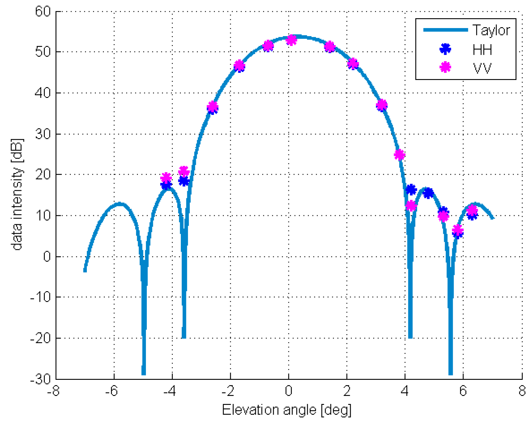
The correctness of the antenna excitation setting and the validation against the theoretical antenna pattern calculation was carried out by repeating the data acquisition with different antenna pointing in elevation thanks to the mechanical steering of the antenna.
Figure 8 below shows an example of the obtained results, where each dot on the plot represents the average power at the moving target range, estimated on one data acquisition, either VV or HH. The dots are superimposed over the theoretical antenna pattern shape, corresponding to the applied tapering on the antenna (Taylor tapering). The good agreement of the measures with the expected pattern can be seen up to the second side-lobe. The agreement is better for positive angles than for negative angles. This can be explained considering the known interaction of the antenna with the ground, introducing a ripple on the whole pattern.
5. Discussion
The execution of the ODT and the processing of the collected data provides an important set of results that give the first significant insights on the overall system performance. First of all, the transmitted signal, after its replica were provided by internal calibration and their similarity to an ideal chirp were checked, showed an almost ideal IRF in range. The compensation of the known phase function, corresponding to the target motion, allowed us to check the phase stability of the system over a long time interval spanning up to 10 min. The analysis over datasets acquired with different azimuth and elevation pointing of the SAOCOM antenna tile allowed the successful validation of the antenna pattern pointing and shape over a large interval including the first and second side-lobes. The main limitations remain the single antenna tile used, thus allowing us to test only the beamforming in the elevation direction, and the target used, which responded only with the co-pol channels. Nevertheless, the collected results allow us to state that the key functionalities of the SAR system are verified, even with the limitations that an on-ground setup unavoidably brings.
6. Conclusions
The SAOCOM-1A outdoor test took place in Bariloche, Patagonia, Argentina, during June 2016.
The main objective of the outdoor test (ODT) was to provide an end-to-end validation of the SAOCOM-SAR functionality, in a realistic condition, where the SAR pulses are radiated by the antenna, reflected by a target, and then received by the antenna and recorded as SAR data. The test setup was made up of two main elements: the SAOCOM SAR engineering model, including one of the seven antenna tiles, and the moving target. It was proven to work as expected throughout the full duration of the tests. Several datasets were successfully acquired through the setup and processed to L0B data.
Overall, the ODT objectives were met and the SAOCOM-1A proved to show an excellent signal quality, both from radiometric and interferometric points of view. The ODT provided the unique occasion to obtain a set of pre-flight far-field measurements. The results can be considered representative for SAOCOM-1A and for SAOCOM-1B as well, so no additional experiments are foreseen. The conclusive and formal verification of the SAOCOM performance is left to the laboratory pre-flight tests and to the commissioning phase.
Acknowledgments
The authors would like to thank CONAE and INVAP for the fruitful cooperation before, during, and after the execution of the outdoor test campaign.
Author Contributions
Andrea Monti Guarnieri originally conceived the experiment. Davide Giudici carried out the feasibility study, coordinated the moving target design and development and processed the acquired SAR data. Juan Pablo Cuesta Gonzalez provided a thorough review of the feasibility study and coordinated the actual setup and execution of the experiment.
Conflicts of Interest
The authors declare no conflict of interest.
References
- SAOCOM Mission Website. Available online: http://www.conae.gov.ar/index.php/english/satellite-missions/saocom/introduction (accessed on 13 July 2017).
- SAOCOM Mission Applications. Available online: http://www.conae.gov.ar/index.php/english/satellite-missions/saocom/technical-characteristics (accessed on 13 July 2017).
- Hees, A.; Koch, P.; Rostan, F.; Huchler, M.; Croci, R.; Østergaard, A. Sentinel-1 Antenna Model Validation: Pattern Prediction vs. PNFS Measurements. In Proceedings of the 2013 IEEE International Symposium on Phased Array Systems and Technology, Waltham, MA, USA, 5–18 October 2013. [Google Scholar]
- Miranda, N.; Meadows, P.; Hajduch, G.; Pilgrim, A.; Piantanida, R.; Giudici, D.; Small, D.; Schubert, A.; Husson, R.; Vincent, P.; et al. The Sentinel-1A Instrument and Operational Product Performance Status. In Proceedings of the 2015 IEEE International Geoscience and Remote Sensing Symposium (IGARSS), Milan, Italy, 26–31 July 2015. [Google Scholar]
- Schwerdt, M.; Schmidt, K.; Ramon, N.T.; Alfonzo, G.C.; Döring, B.J.; Zink, M.; Prats-Iraola, P. Independent Verification of the Sentinel-1A System Calibration. IEEE J. Sel. Top. Appl. Earth Obs. Remote Sens. 2016, 9, 994–1007. [Google Scholar] [CrossRef]
- Iannini, L.; Guarnieri, A.M. Atmospheric phase screen in ground-based radar: Statistics and compensation. IEEE Geosci. Remote Sens. Lett. 2011, 8, 537–541. [Google Scholar] [CrossRef]
Figure 1.
SAOCOM outdoor test (ODT) concept overall view. In the figure, P represents the moving target to be acquired and ϑ the inclination of the Radar Line of Sight with respect to the local normal to the terrain.
Figure 1.
SAOCOM outdoor test (ODT) concept overall view. In the figure, P represents the moving target to be acquired and ϑ the inclination of the Radar Line of Sight with respect to the local normal to the terrain.

Figure 2.
SAOCOM-1A outdoor test setup. (a) View on map; (b) aerial photo.

Figure 3.
(a) Radome hosting the SAOCOM antenna tile; (b) Radome hosting the moving target.
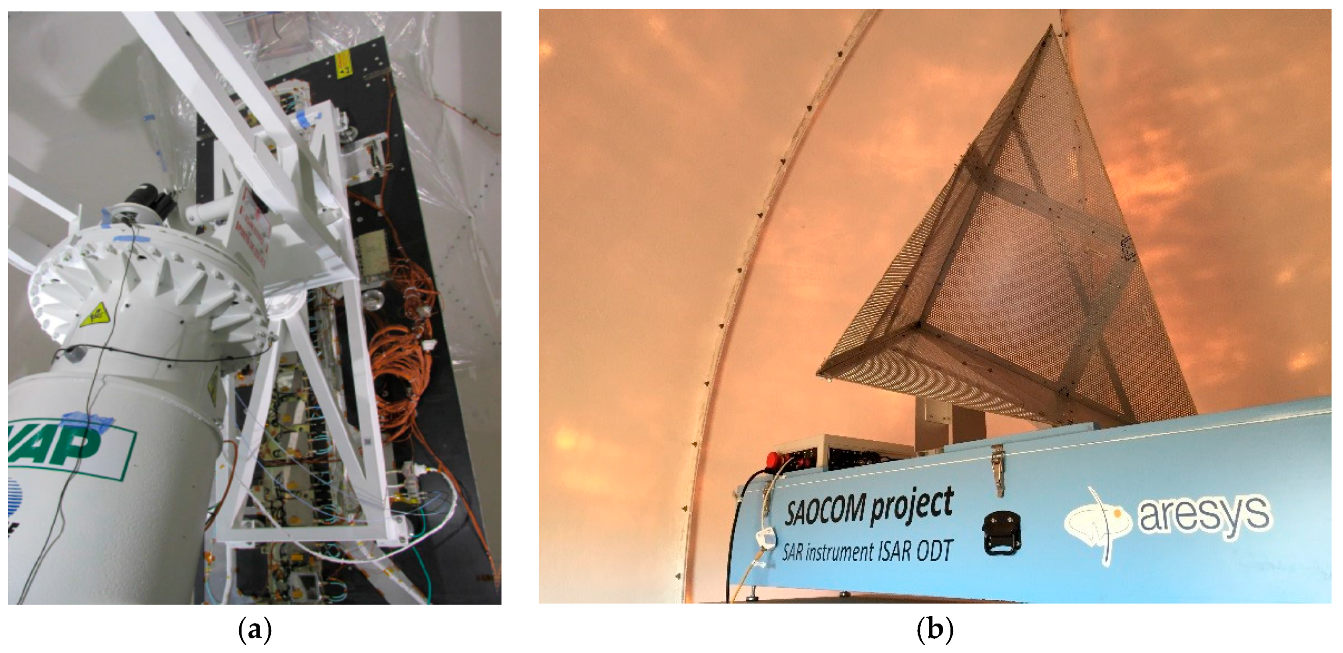
Figure 4.
(a) Comparison between the ideal chirp and the chirp extracted from internal calibration; (b) Range-compressed Impulse Response Function (IRF) comparison.
Figure 4.
(a) Comparison between the ideal chirp and the chirp extracted from internal calibration; (b) Range-compressed Impulse Response Function (IRF) comparison.

Figure 5.
(a) Range-compressed data intensity profile and interpretation; (b) Doppler analysis of the clutter.
Figure 5.
(a) Range-compressed data intensity profile and interpretation; (b) Doppler analysis of the clutter.

Figure 6.
(a) Range-Doppler map with the focused moving target clearly visible; (b) Azimuth IRF.
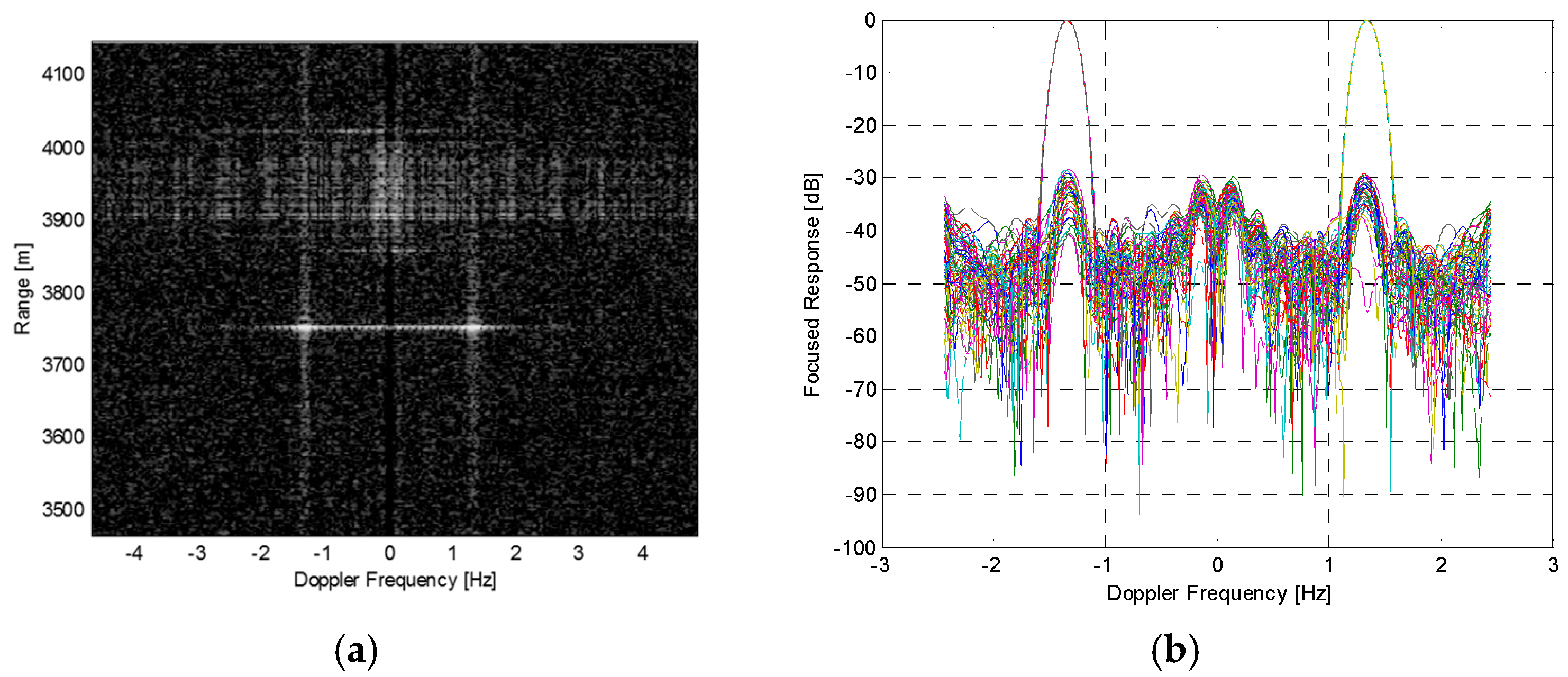
Figure 7.
Analysis of the moving target signal. (a) Phase versus time; (b) Doppler frequency versus time (colorscale in dB, normalized to the maximum); (c) Residual phase after linear motion compensation.
Figure 7.
Analysis of the moving target signal. (a) Phase versus time; (b) Doppler frequency versus time (colorscale in dB, normalized to the maximum); (c) Residual phase after linear motion compensation.
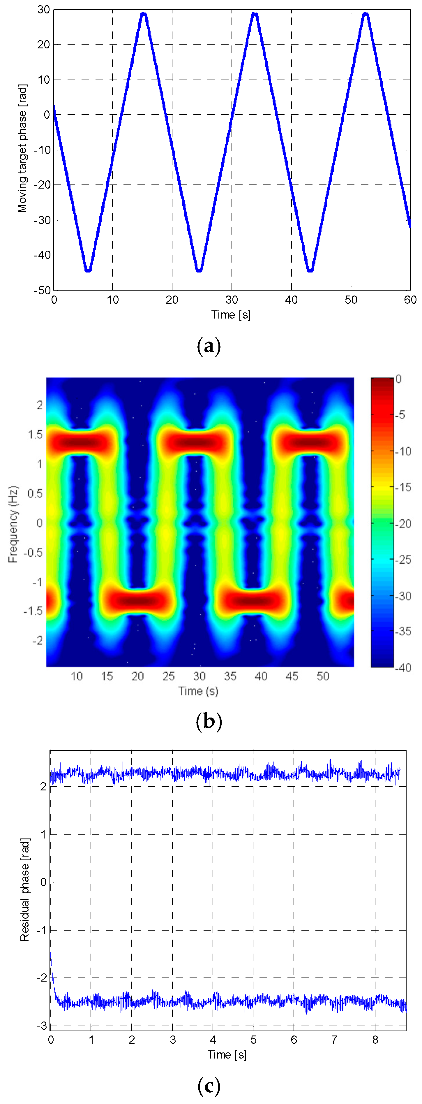
Figure 8.
Far-field elevation antenna pattern validation against the theoretical model.


Table 1.
Radar Cross Section (RCS) of the corner reflectors.
| 75 cm Corner RCS | 100 cm Corner RCS | 150 cm Corner RCS |
|---|---|---|
| 13.79 dBsm | 18.79 dBsm | 25.83 dBsm |
Table 2.
Link budget computation and Signal to Noise Ratio (SNR) computation (ideal propagation media).
Table 2.
Link budget computation and Signal to Noise Ratio (SNR) computation (ideal propagation media).
| Parameter | Value (Linear) | Value (Log-Scale) |
|---|---|---|
| Peak power | 750.0 W | 28.75 dBW |
| Antenna area transmit (TX) | 4.87 m2 | 6.88 dBsm |
| Instrument and antenna TX losses | 1.17 | 0.70 dB |
| TX path loss (R = 3755 m) | 5.64 × 10⁻⁹ | −82.48 dB |
| RCS corner (1-m corner case) | 75.66 m2 | 18.79 dBsm |
| Receive (RX) path loss | 5.64 × 10⁻⁹ | −82.48 dB |
| Instrument and antenna RX losses | 1.17 | 0.70 dB |
| Received power | 6.4 × 10⁻¹² W | −111.94 dBW |
| Noise figure | 2.14 | 3.3 dB |
| Noise power at receiver | 4.28 × 10⁻¹³ W | −123.69 dBW |
| SNR raw | 14.96 | 11.75 dB |
| Number of focused steps | 1000 | 30 dB |
| SNR focused | 14,962 | 41.75 dB |
Table 3.
SAOCOM 1A acquisition parameters for outdoor test.
| Parameter | Value |
|---|---|
| Acquisition mode | Stripmap/TOPSAR |
| Center frequency | 1,274,140,000 Hz |
| Bandwidth | 50 MHz |
| Sampling window start time | 23 μs |
| Chirp duration | 11 μs |
| Sampling window length | 20 μs |
| Acquisition duration | variable 1 min–10 min |
| Polarization | Quad Pol |
| Pulse Repetition Frequency (PRF) | 4545 Hz |
| Chirp | Down |
Table 4.
Range IRF analysis results.
| IRF Parameter | Replica-Replica Case | Ideal-Ideal Case | Replica-Ideal Case |
|---|---|---|---|
| Resolution | 2.77 m | 2.66 m | 2.68 m |
| Peak-to-Side-Lobe ratio | −16.2 dB | −13.3 dB | −14.98 dB |
Table 5.
Amplitude and phase stability results over 10 min.
| Parameter | Value (VV) | Value (HH) |
|---|---|---|
| Amplitude stability | better than 0.1 dB | better than 0.1 dB |
| Phase stability | 3.9 deg | 3.4 deg |
| Amplitude drift | <0.1 dB/min | <0.1 dB/min |
| Phase drift | 0.19 deg/min | 0.35 deg/min |
© 2017 by the authors. Licensee MDPI, Basel, Switzerland. This article is an open access article distributed under the terms and conditions of the Creative Commons Attribution (CC BY) license (http://creativecommons.org/licenses/by/4.0/).
Share and Cite
MDPI and ACS Style
Giudici, D.; Monti Guarnieri, A.; Cuesta Gonzalez, J.P. Pre-Flight SAOCOM-1A SAR Performance Assessment by Outdoor Campaign. Remote Sens. 2017, 9, 729. https://doi.org/10.3390/rs9070729
AMA Style
Giudici D, Monti Guarnieri A, Cuesta Gonzalez JP. Pre-Flight SAOCOM-1A SAR Performance Assessment by Outdoor Campaign. Remote Sensing. 2017; 9(7):729. https://doi.org/10.3390/rs9070729
Chicago/Turabian StyleGiudici, Davide, Andrea Monti Guarnieri, and Juan Pablo Cuesta Gonzalez. 2017. "Pre-Flight SAOCOM-1A SAR Performance Assessment by Outdoor Campaign" Remote Sensing 9, no. 7: 729. https://doi.org/10.3390/rs9070729
Note that from the first issue of 2016, this journal uses article numbers instead of page numbers. See further details here.