
Comparing Sentinel-2A and Landsat 7 and 8 Using Surface Reflectance over Australia

Joint Remote Sensing Research Program, School of Earth and Environmental Sciences, University of Queensland, St. Lucia, QLD 4072, Australia
Remote Sens. 2017, 9(7), 659; https://doi.org/10.3390/rs9070659
Submission received: 5 May 2017
/
Revised: 22 June 2017
/
Accepted: 25 June 2017
/
Published: 27 June 2017
Abstract
:The new Sentinel-2 Multi Spectral Imager instrument has a set of bands with very similar spectral windows to the main bands of the Landsat Thematic Mapper family of instruments. While these should, in principle, give broadly comparable measurements, any differences are a function not only of the differences in the sensor responses, but also of the spectral characteristics of the target pixels. In order to test for and quantify differences between these sensors, a large set of coincident imagery was assembled for the Australian landscape. Comparisons were carried out in terms of surface reflectance, and also in terms of biophysical quantities estimated from the reflectances. Small but consistent differences were found, and suitable adjustment equations fitted to enable transformation of Sentinel-2A reflectance values to more closely match Landsat-7 or Landsat-8 values. This is useful if trying to take models and thresholds fitted from Landsat and use them with Sentinel-2. The fitted adjustment equations were also compared against those fitted globally for NASA’s Harmonized Landsat-8 Sentinel-2 product, and found to be substantially different, raising the possibility that such adjustments need to be fitted on a regional basis.

1. Introduction
The Sentinel satellite constellation of the European Space Agency (ESA) includes several satellite families, as part of their Copernicus programme of Earth observation. The Sentinel-2 family carries a single instrument called the Multi Spectral Instrument (MSI), which is a high-resolution optical instrument, with spectral characteristics similar to both the SPOT (Satellite Pour l’Observation de la Terre) and Landsat families [1]. It improves on these by having higher spatial resolution than Landsat, and more spectral bands and greater revisit frequency than either. The long term plan is to launch and maintain a series of Sentinel-2 satellites (named 2A, 2B, etc.), over many years, with Sentinel-2A launched on 23 June 2015, and Sentinel-2B launched on 7 March 2017. They each have a planned lifetime of seven years, and further launches are planned with the same instrument in later years.
The MSI instrument has a total of 13 spectral bands, at different spatial resolutions. There are four visible and near infra-red bands at 10 m pixel size, roughly corresponding to equivalent Landsat Thematic Mapper (TM) bands, and six near infra-red bands and short wave infra-red bands at 20 m pixel size. The orbit and swath width mean that the nominal revisit time for a single satellite is 10 days. When two satellites are operating, they will be out of phase so that the nominal revisit time over both satellites will be five days [1] (subject to the ESA’s acquisition scheduling). Areas that are in the overlap between swaths will obviously be revisited more often.
The Landsat family of satellites has provided a long record of earth observation stretching over 40 years, and much existing work has been developed from their data [2,3]. In order to build on this record, it will be useful to be able to combine imagery acquired by the two families of instruments, and perhaps more importantly to transfer thresholds and fitted models trained on Landsat data for use with the higher resolution imagery of Sentinel-2. This raises the question of how comparable the different sensors are, and what impact the difference would have on models of biophysical quantities. Mandanici and Bitelli [4] explored these questions in a small study of five image pairs, and pointed to the need for larger studies. Vuolo et al. [5] presented work on a complete system for producing surface reflectance and a number of biophysical products from Sentinel-2, and included some comparison of surface reflectance with that generally available for Landsat-8 (the United States Geological Survey Climate Data Record product), for six test sites in Europe. Their results show that the agreement between the two products is good, reporting Root Mean Square error values on the order of 0.03 reflectance units, and this speaks well of the systems these workers have set up. However, since the Sentinel-2 and Landsat-8 products used were created using different surface reflectance transformation algorithms, it is not possible to assess the extent to which the differences are a direct result of the sensor responses or the differences in processing methods. NASA have released documentation for a combined product merging Landsat-8 and Sentinel-2 imagery, called the Harmonized Landsat-8 Sentinel-2 Product (HLS). In creating this product, they have also explored the comparability of these two sensors, and published linear adjustment functions to transform Sentinel-2 reflectance to Landsat-8 reflectance [6]. These adjustment functions were based on hyperspectral spectra taken from 500 sites in a global dataset, combined with the spectral response functions of the two sensors.
Since Landsat-5 failed in late 2011, there is no opportunity to acquire Sentinel-2 imagery coincident with that. However, both Landsat-7 and Landsat-8 are still operational and there is now a considerable period in which data have been acquired from Sentinel-2A, Landsat-7 and Landsat-8. This article uses hundreds of these coincident acquisitions, from a large area of the Australian continent, to perform a direct comparison of the surface reflectances from these instruments, and quantify the differences between Sentinel-2A and the two Landsat instruments. It also presents some analysis showing the impact of these differences on two models used to estimate biophysical quantities.
It should be noted that the differences in response are dependent on the nature of the target being observed, and so this study is first and foremost applicable to the Australian landscape.
The techniques used here closely follow those used by Flood [7] when comparing Landsat-8 Operational Land Imager (OLI) with Landsat-7 Enhanced Thematic Mapper+ (ETM+).
2. Methods
2.1. Comparison Dataset
The differing orbits and swath widths of Landsat and Sentinel-2 mean that it is possible to find many instances in which the two satellites observe the same ground locations on the same day. Since both satellites are sun-synchronous with mid-morning overpass time, these pairs of observations are generally only minutes apart, and it can therefore be assumed that there is no change in the land surface occurring between the two observations. Atmospheric conditions are also unlikely to have changed significantly between the two acquisitions. This implies that any differences found between the two observations are due solely to the differences in the sensors, or the observation conditions, rather than a change in the target.
It is important to note that the orbits and swath widths of the two instruments can imply significant differences in view angle. These paired observations could involve a nadir observation from one instrument paired with an edge-of-swath observation from the other instrument. Hence, there is also potential for considerable variation in atmospheric path length, and variation in the effects of the Bi-direction Reflectance Distribution Function (BRDF), and so the differences in observation conditions could be of some importance.
In order to minimize differences due to observation conditions, the imagery for both sensors was standardized to surface reflectance at a standard observation geometry, using the methods described by Flood et al. [8]. This transforms the imagery by correcting for atmospheric effects and the effects of the Bidirectional Reflectance Distribution Function (BRDF), and presents surface reflectance at nadir view and a solar zenith angle of . The spectral response functions supplied by the ESA for Sentinel-2A were added to the atmospheric correction code (Second Simulation of the Satellite Signal in the Solar Spectrum, known as 6S [9]), so that the identical radiometric processing was used for all sensors. Aerosol optical thickness (AOT) in Australia tends to be very low by global standards, and is assumed to be a constant low value of 0.05 [10,11]. While this value would not be realistic in many other parts of the world, this is not important to the comparisons at hand. The important point is that the same value is used for all sensors.
It is then assumed that any remaining difference between observations is due solely to the difference in the sensor responses to the pixels in question.
The bands used for comparison were those that correspond most closely between the different instruments. The correspondence is given in Table 1. While the Sentinel-2 Near Infra-Red (NIR) band 8A has a spectral response which corresponds more closely to that of Landsat-8 OLI, this band is available at only 20 m pixel size, and so it is not likely that this would be the band in major use for studies working at 10 m resolution. In addition, the Landsat-7 ETM+ NIR band is wider, and covers roughly the same window as the Sentinel-2 band 8. Thus, for these reasons, only Sentinel-2 band 8 was considered for NIR correspondence.
A random selection of points was chosen across a large part of continental Australia. These were chosen on the basis of the tiling used by the ESA for distribution of Sentinel-2 data, with a random selection of unmasked points within each tile contributing to the whole dataset, to ensure an even distribution of points across the landscape. From this set of points, one third were set aside as validation, while the rest were used for fitting of the prediction models described below. All of the comparisons shown in Section 4 were carried out using the validation dataset.
The 10 m and 20 m Sentinel-2 bands were resampled to match the 30 m pixels of the corresponding Landsat imagery, using the “average” resampling method provided in the gdalwarp software (version 1.11.5) [12].
2.2. Comparison Methods
The resampled Sentinel-2 pixel values were compared separately with corresponding pixels of Landsat-7 and Landsat-8 from same-day acquisitions. Scatter plots are used to display the corresponding bands. On all plots, the Sentinel-2 version of the variable is shown on the x-axis, while the Landsat version is shown on the y-axis. Each scatter plot shows the 1-to-1 line (solid line) representing perfect agreement between the two sensors. In addition, each plot shows a number of statistics which summarize the variation between the two variables.
The slope of the Orthogonal Distance Regression (ODR) line is used to capture the proportional relationship between the x and y values. This fits a line through the data and intersecting the origin, and this line is plotted as a dashed line on the scatter plots. The slope of this line is a simple summary statistic that shows the average behaviour of the ratio of x and y in a robust manner. This is useful because, in general, for the quantities being discussed here, the value of the difference between x and y is proportional to the x and y values themselves. This captures and quantifies the intuitive notion of drawing a line from the origin through the centre of the points on the scatter plot, and seeing how far away that lies from the 1-to-1 line. Orthogonal Distance Regression treats the two variables symmetrically, without assuming that all noise is limited to the independent variable (as is the case with Ordinary Least Squares regression). Perfect agreement between sensors would have a slope value of 1.0.
The Pearson correlation coefficient (r) is also shown on each scatter plot. This is a measure of the linear correlation between the two variables, independent of scaling factors and offsets between them. It is thus a very direct measure of the amount of scatter on the scatter plots. Perfectly correlated variables will have a correlation value of 1.0, while two variables with no linear relationship at all will have a correlation of 0.0.
The root mean square error (RMSE) between x and y is also shown on each scatter plot. This is a measure of the absolute difference between the values of x and y. It is affected by a number of different factors, including the amount of scatter, any offset between the two variables, and scaling differences. This is a good measure of the variation between x and y, but does not distinguish between these different types of variation.
To fit prediction models, Ordinary Least Squares regression was used, to create a mapping from Sentinel-2A reflectance to Landsat reflectance. A separate model, of the form shown in Equation (1), was fitted for each band
where represents surface reflectance for the given instrument, at a given wavelength, and the parameters and are fitted independently for each band.
In addition to comparing the reflectances, comparisons were also performed to show the effect of these reflectance differences when the reflectance values are used to estimate biophysical quantities. A spectral unmixing model of vegetation cover fractions was used to estimate the proportions of green vegetation, non-green vegetation, and bare soil in each pixel. This model was originally fitted using historic Landsat data, using surface reflectance as input [13,14], and was used with the adjustment equations derived by Flood [7] to account for the differences between Landsat-7 and Landsat-8.
A simpler, but more commonly used indicator of green vegetation cover is the Normalized Difference Vegetation Index (NDVI) (reviewed by Bannari et al. [15]). NDVI is calculated using the NIR and Red bands, as shown in Equation (2)
where and are the reflectances in the NIR and Red bands, respectively.
Comparisons were performed for both the fractional cover model and the NDVI. Results are presented for the case when using the unmodified reflectances, and for using the reflectances when adjusted using Equation (1).
2.3. NASA’s Harmonized Landsat-8 Sentinel-2 Product (HLS)
The United States National Aeronautics and Space Administration (NASA) have released a product which combines Landsat-8 and Sentinel-2 imagery in a consistent form. For this purpose, they have fitted linear equations to adjust the surface reflectance of each Sentinel-2 band to match the corresponding Landsat-8 band. However, their approach was to simulate the two instruments from hyperspectral data collected by the Hyperion instrument [16], from 500 individual sites around the world. This has the advantage of being generated from exactly the same data, so there is no possibility of differences due to change on the ground, or differences in observation conditions. Pearlman et al. [16] show that this kind of technique is capable of simulating the data observed from orbit by Landsat-7, and, in principle, this should be true more widely.
The User’s Guide to version 1.2 of the HLS product [6] gives the coefficients fitted to this simulated dataset, which use the same equation as used here (Equation (1)) to adjust Sentinel-2 surface reflectance to match Landsat-8. In principle, this should be equivalent to the adjustment procedure outlined here. To test the consistency of these two models, the HLS adjustment was tested here on the same dataset, to see whether it also reduces the difference between the two instruments. The coefficients used for adjustment in the HLS product are reproduced here in Table 2.
The HLS project chose to use the Sentinel-2 band 8A for their NIR band, as opposed to band 8 used in the current work (see Section 2.1). For this reason, comparing the adjustments for the NIR band is meaningless, and these are not included in the comparisons presented.
3. Data
All Landsat data was downloaded from the USGS EarthExplorer website [17], as level L1T data. The imagery gaps from the failed Scan Line Corrector in Landsat-7 were treated as null areas (i.e., not gap-filled), and did not contribute to the analysis. All data was from pre-collection legacy datasets, as opposed to the newer Collection-1 data introduced during late 2016 and early 2017.
All Sentinel-2A data was downloaded from the ESA as Standard Archive Format for Europe (SAFE) format zip files of level L1C data [18]. Only data processed with the ESA’s version 02.04 system was used, as per the ESA’s recommendations due to errors in their earlier processing software. The data was that available by February 2017. Thanks to the ESA’s reprocessing efforts, there was, by this time, a large quantity of earlier imagery available as 02.04-processed output.
The data searched for was from the entire holdings of Sentinel-2 imagery in the Remote Sensing Centre of the government of the Australian state of Queensland, where this work was undertaken, and covers around two thirds of the land mass of Australia.
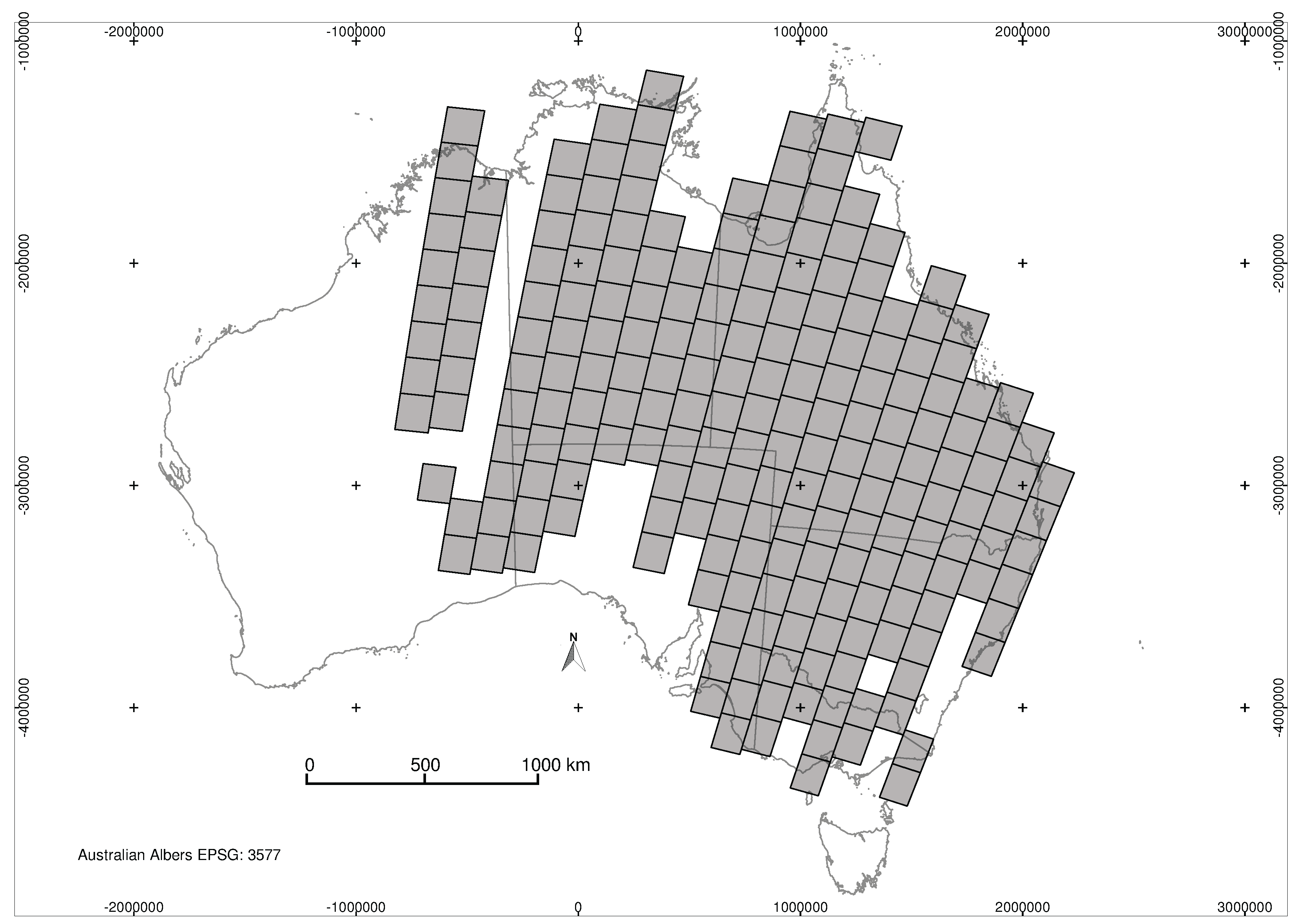
Imagery dates were in the period from August 2015 to January 2017. For the Landsat-7 comparison, there were 46 distinct cloud-free dates across 178 distinct scenes, while for the Landsat-8 comparisons, there were 49 distinct dates across 174 scenes. The average number of dates for each scene was 4.9 for Landsat-7, and 4.4 for Landsat-8. The Landsat scenes used are shown in Figure 1.
Cloud and cloud shadow masking was performed using Fmask [19,20]. The percentage cloud cover given by this method was used to select only dates that had less than 1% cloud. This was done in order to minimize the likely impact of undetected cloud and cloud shadow, recognising that the Fmask algorithm does not create a perfect mask. As a final filter to remove remaining undetected cloud or shadow, the ratio of the blue band in the two sensors was calculated. Any points for which this ratio was larger than 2 or smaller than 0.5 were removed, on the assumption that these represent pixels that were clear in one image but brightened by cloud or darkened by shadow in the other image. This removed approximately 0.5% of pixels.
Topographic shadow masking was performed using the methods described by Robertson [21], and areas deemed to be in shadow were excluded from consideration. Areas of water were masked using the methods described by Fisher et al. [22], and omitted from consideration.
The final number of points used in each comparison exercise is shown in Table 3.
Each point in these counts is a single 30 m pixel on a single date. It is assumed that there is no registration error between sensors. Visual inspection suggests that this is not entirely true. A small study by Yan et al. [23] also indicates registration errors for imagery in South Africa, and suggests that the cause relates to the quality of ground control points used to register Landsat. Such registration errors would be dependent on location, and in the absence of a large assessment of Sentinel-Landsat co-registration errors in Australia, the assumption is made that such errors would not contribute to any apparent systematic bias in reflectance values. They could certainly increase the scatter in the comparisons, but it is difficult to see any way in which it could be so consistent as to affect the average behaviour over a large area. In any case, it is beyond the scope of this analysis to attempt to assess or improve on the registration. The ESA are planning to re-process all of their Sentinel-2 imagery with an improved ground reference image, but this has not yet been put in place for processing of Australian imagery [24].
4. Results
Table 4 gives the coefficients fitted for Equation (1), for each band and sensor combination. The coefficients were fitted using Ordinary Least Squares regression, and as such are specifically for estimating Landsat reflectance from Sentinel-2A reflectance. They should not be inverted to use in the reverse sense.
4.1. Surface Reflectance
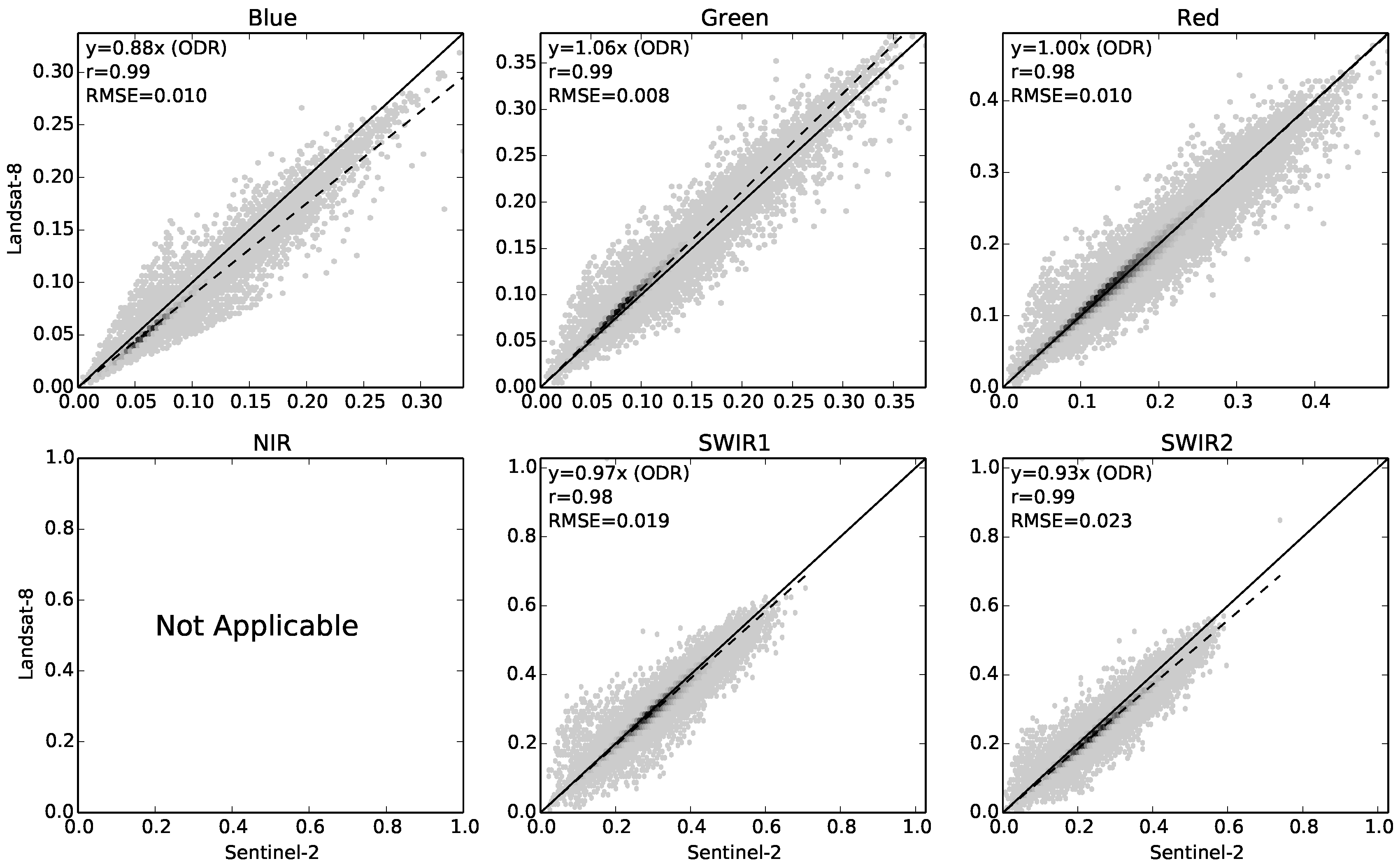
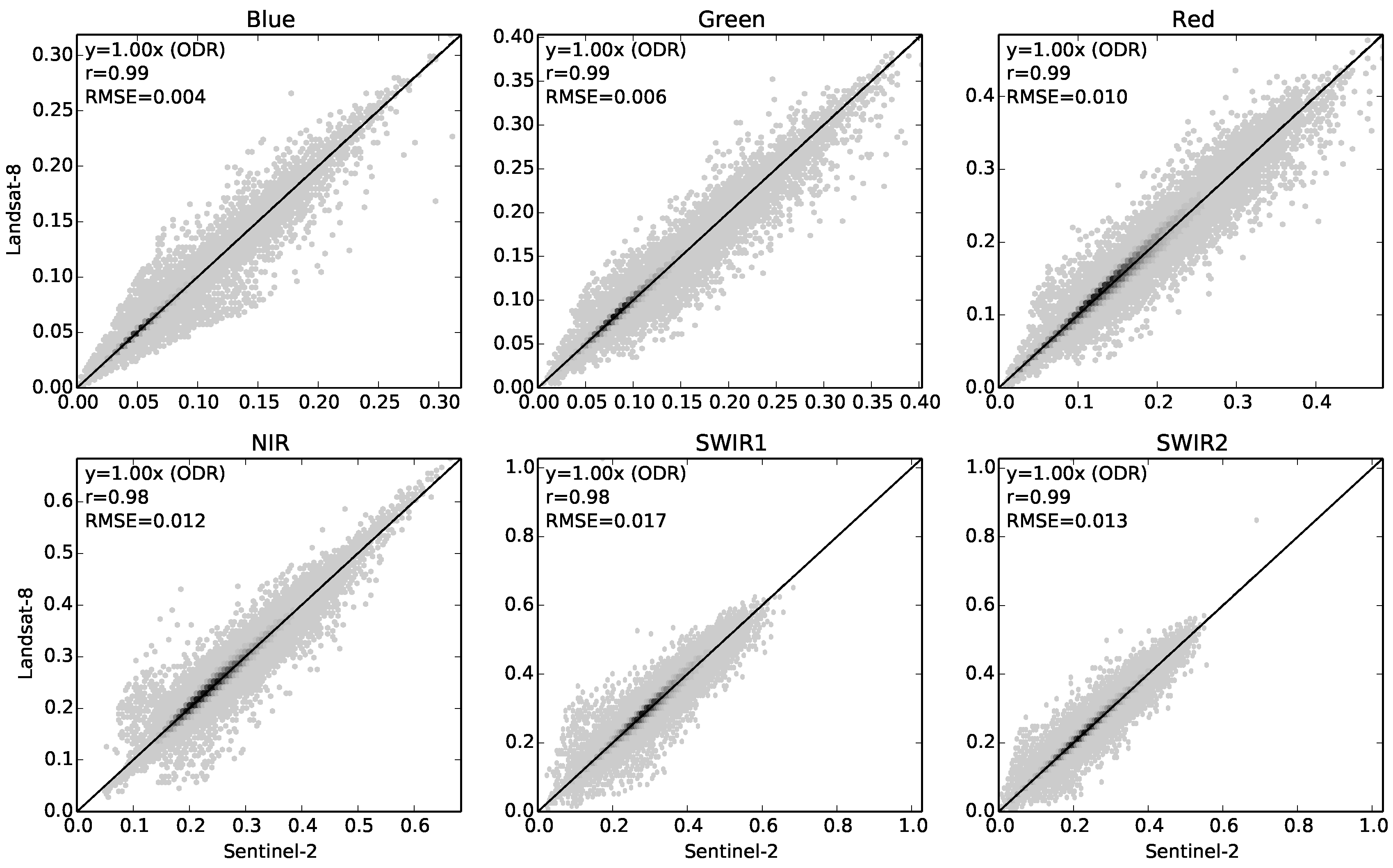
The scatter plots in Figure 2 and Figure 3 show that there are consistent differences between Sentinel-2A and both of the Landsat sensors. The differences appear to be proportional to the reflectance magnitude, with minimal constant offset. Depending on which band, the ODR slope statistic ranges from 0.93 to 1.09 and the RMSE ranges from 0.005 to 0.021.
There is a certain amount of scatter evident in all scatter plots, but the regions shown as darker, representing the majority of the pixels, are much less scattered. This is supported by the Pearson correlation values, which are all in the range 0.97 to 0.99.
Figure 2 shows the direct comparison of corresponding bands between Sentinel-2A and Landsat-7. Figure 3 shows the equivalent comparison of Sentinel-2A with Landsat-8. Very similar patterns appear, although the amount of difference is slightly dependent on which Landsat is being compared. This is consistent with earlier work suggesting that Landsat-7 and Landsat-8 are not identical instruments but exhibit systematic variation between the two sensors [7,25,26].
Figure 4 and Figure 5 show the same reflectance comparisons, after applying the fitted adjustment using Equation (1), with coefficients from Table 4. Unsurprisingly, the adjustment brings the data back to the 1-to-1 line, removing systematic between-sensor variation in either direction. All the ODR slope statistics are equal to 1 (within two decimal places). The RMSE values are all reduced by the adjustment, except for Landsat-8 Red band, which remains the same. It is worth emphasizing that the coefficients used for the adjustment were fitted on a separate set of points. As discussed in Section 2.1, the extracted point data was randomly split into training and validation subsets. The coefficients were fitted on the training points, but the comparisons presented here are from the validation points, which are quite distinct, while still coming from the same regional population.
4.2. Fractional Cover
The scatter plots in Figure 6 show the effect of the differences in reflectance when used with a model of a fractional vegetation cover. The comparison presented here is for Sentinel-2A with Landsat-8. The Landsat-7 case is omitted here for the sake of brevity, but exhibits nearly identical effects.
Over the three vegetation cover fractions, the ODR slope statistics range from 0.97 to 1.07, and RMSE ranges from 0.040 to 0.054. Since the cover fractions must sum to 1, obviously an increase in one fraction produces a corresponding decrease in one of the others. There is noticeably more scatter in these plots than in the reflectance plots (with r values as low as 0.95), possibly as a result of the strongly non-linear nature of the fractional cover model. However, there is still a systematic between-sensor variation in all three fractions.
Figure 7 shows the same comparisons, but when the reflectances have first been adjusted using Equation (1), before being used in the fractional cover model. With this adjustment, the ODR slope statistics range from 0.99 to 1.00, for all three cover fractions, and all of the RMSE values are reduced by the adjustment.
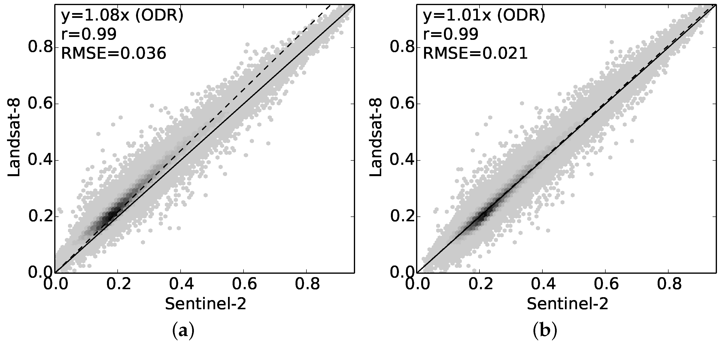
4.3. NDVI
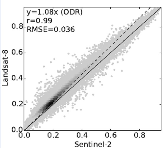
Figure 8a shows the comparison of the NDVI values calculated from Sentinel-2A and Landsat-8. The ODR slope statistics is 1.08, and the RMSE is 0.036. In Figure 8b, the same comparison is presented, but after adjusting the reflectances using Equation (1). The ODR slope is reduced to 1.01, and the RMSE is reduced to 0.021.
The Landsat-7 case is omitted here for the sake of brevity, but exhibits nearly identical behaviour.
4.4. Surface Reflectance Adjusted Using HLS Coefficients
Inspection of the coefficients calculated here (Table 4, Landsat-8 entries) and those calculated for HLS (Table 2) suggests that they appear to be very different. In principle, one might expect the HLS coefficients to be similar to those found here for Landsat-8, but, in most bands, the regression slopes () do not even adjust in the same direction. In all bands except SWIR1, those values which HLS gives as greater than 1 are found here to be less than 1, and vice versa. This suggests that the two adjustment models are not consistent with each other.
The adjustment procedure to map Sentinel-2A to match Landsat-8, as shown in Figure 5, was repeated for the same dataset, but using the coefficients fitted for NASA’s HLS product (reproduced here in Table 2). In principle, if the two adjustment models are equivalent, then the results should be similar to Figure 5. The comparison of the adjusted Sentinel-2A reflectances with Landsat-8 is shown in Figure 9.
This shows that, in most bands, the resulting agreement is not noticeably closer to 1-to-1. In the red band, the ODR slope has changed from 1.01 to 1.00, but in most other bands, they remain around the same as for the unadjusted data. In the blue band, the ODR slope has worsened from 0.95 to 0.88.
5. Discussion
The comparisons shown in Figure 2 and Figure 3 demonstrate that the agreement between the corresponding bands of Sentinel-2A and Landsat sensors is very good, but there are small consistent variations between them. In all bands, for both Landsat sensors, the bulk of the data (shown as the darker areas of each scatter plot) is very close to the 1-to-1 line, but does not lie exactly along it, with with ODR slope statistics in the range 0.93 to 1.09, depending on the band. For many purposes, this would be quite sufficient agreement to work with combinations of both instruments, or to use with existing Landsat-derived models. However, in some contexts, the differences could be sufficient to create small persistent variations between the Landsat and Sentinel data.
Applying an adjustment with Equation (1) to these reflectance values brings the between-sensor ODR slopes to 1.00, in all cases. This adjustment of reflectances also removes the systematic variations in the outputs of the fractional vegetation cover model, and from the NDVI values calculated from the surface reflectance values. This makes it possible to take models and thresholds which were fitted using Landsat data, and apply them to the reflectance values from Sentinel-2A, and have some confidence that the new sensor is not introducing a systematic offset or scaling difference.
The particular methods used here to estimate surface reflectance will have the same strengths and weaknesses for all the sensors. As mentioned in Section 2.1, the correct spectral response functions for Sentinel-2A were added to the system, and all other factors were kept the same. For the purposes of comparison, the main point is that it provides a consistent framework in which to compare surface reflectance between the sensors.
The comparisons of surface reflectance do show a certain amount of scatter. There are a number of possible causes for this, including image mis-registration, and viewing geometry effects such as BRDF and atmospheric path length, which might not be fully accounted for by the transformation to surface reflectance. The viewing geometry can be markedly different between sensors, due to the different swath arrangements and resulting view angles. However, it must be accepted that one probably significant factor is that, on any given pixel, the response to the different sensors differs in ways which are specific to that pixel. This would involve details of the pixel’s spectral characteristics in regions of the spectral window where the two sensors have different spectral response, and is not directly predictable from the sensor response functions alone. This component of the between-sensor difference cannot be removed using the sorts of methods described and tested here, and is likely to remain a part of any attempts to combine imagery from multiple sensors.
These per-pixel differences also raise the possibility that consistent regional differences may also exist. The work presented by Flood [7] showed that this was true for the case of comparing Landsat-7 against Landsat-8, but that the differences within the Australian landscape appear to be smaller than the average between-sensor differences across the whole landscape (Table 3 in Flood [7]).
The comparison of the adjustments fitted here against those fitted for the HLS project also raises the question of regional differences, on a larger scale. The most likely explanation for the substantial difference in the adjustments is that the HLS coefficients were fitted on a global dataset, potentially dominated by land surfaces not representative of those common in Australia. The distribution of training points is shown in the map at the HLS website [6]. If this is the explanation, then it suggests that caution should be exercised before using a global adjustment for this purpose, and that, at the very least, such an adjustment should be tested for a particular region before accepting it as suitable. A good test of this hypothesis would be to use regional subsets of the global Hyperion spectra dataset to fit adjustments per region, and test how compatible they are. This is similar to the technique used by Flood [7] to test the variability across the Australian region.
Another possible explanation for the difference between the adjustments fitted here and those fitted by HLS may be that they are based on different methods for transforming to surface reflectance. As discussed above, the most important factor is to use the same method for the two instruments, so that it does not add any apparent difference between instruments. However, if the adjustment factors fitted for transforming Sentinel-2 to Landsat are strongly dependent on the nature of the surface reflectance transformation used, this would also suggest that caution is required before using the HLS coefficients on any other data than that used by their project. In particular, when ESA settles on a standard surface reflectance algorithm for their Level 2 product, it may be unwise to apply the HLS coefficients to transform it to match Landsat-8. In order to test this hypothesis, it seems likely that careful experimentation with a number of different surface reflectance approaches would be required.
6. Conclusions
This comparison of Sentinel-2A and Landsat 7 and 8 shows that the new instrument has very good compatibility with the existing Landsat instruments. However, it does also show that there are some small but systematic differences, which could be important in some contexts. These differences are in the range 1% to 9%, depending on the band in question.
Simple adjustment equations were derived for each of the corresponding bands, which enable adjustment of Sentinel-2A surface reflectance to match either Landsat-7 or Landsat-8, as required. These adjustments bring the average systematic difference to less than 1% in all bands.
It was also shown that the differences in reflectance carry through to produce corresponding differences in estimates of biophysical quantities such as green vegetation cover, with systematic differences of up to 8%. However, adjusting the reflectances as discussed was able to reduce this to around 1%, on average. This increases the confidence with which one might transfer models and thresholds from Landsat, for use with Sentinel-2 imagery.
The comparison of the adjustments fitted here with those fitted for the Harmonized Landsat-8 Sentinel-2 product suggests that there may be substantial regional variation implicit in such adjustments, and that they should be tested locally when used in a specific region.
Acknowledgments
The Joint Remote Sensing Research Program is supported financially by the governments of the Australian states of Queensland and New South Wales.
Conflicts of Interest
The author declares no conflict of interest.
References
- Drusch, M.; del Bello, U.; Carlier, S.; Colin, O.; Fernandez, V.; Gascon, F.; Hoersch, B.; Isola, C.; Laberinti, P.; Martimort, P.; et al. Sentinel-2: ESA’s Optical High-Resolution Mission for GMES Operational Services. Remote Sens. Environ. 2012, 120, 25–36. [Google Scholar] [CrossRef]
- Roy, D.; Wulder, M.; Loveland, T.; Allen, R.; Anderson, M.; Helder, D.; Irons, J.; Johnson, D.; Kennedy, R.; Scambos, T.; et al. Landsat-8: Science and product vision for terrestrial global change research. Remote Sens. Environ. 2014, 145, 154–172. [Google Scholar] [CrossRef]
- Loveland, T.R.; Dwyer, J.L. Landsat: Building a strong future. Remote Sens. Environ. 2012, 122, 22–29. [Google Scholar] [CrossRef]
- Mandanici, E.; Bitelli, G. Preliminary Comparison of Sentinel-2 and Landsat 8 Imagery for a Combined Use. Remote Sens. 2016, 8, 1014. [Google Scholar] [CrossRef]
- Vuolo, F.; Żółtak, M.; Pipitone, C.; Zappa, L.; Wenng, H.; Immitzer, M.; Weiss, M.; Baret, F.; Atzberger, C. Data service platform for Sentinel-2 surface reflectance and value-added products: System use and examples. Remote Sens. 2016, 8, 938. [Google Scholar] [CrossRef]
- Claverie, M.; Masek, J.; Ju, J. Harmonized Landsat-8 Sentinel-2 (HLS) Product User’s Guide, 2016. Available online: https://hls.gsfc.nasa.gov/wp-content/uploads/2017/03/HLS.v1.2.UserGuide.pdf (accessed on 1 April 2017).
- Flood, N. Continuity of Reflectance Data between Landsat-7 ETM+ and Landsat-8 OLI, for both top-of-atmosphere and surface reflectance: A Study in the Australian landscape. Remote Sens. 2014, 6, 7952–7970. [Google Scholar] [CrossRef]
- Flood, N.; Danaher, T.; Gill, T.; Gillingham, S. An Operational Scheme for Deriving Standardised Surface Reflectance from Landsat TM/ETM+ and SPOT HRG Imagery for Eastern Australia. Remote Sens. 2013, 5, 83–109. [Google Scholar] [CrossRef]
- Vermote, E.; Tanre, D.; Deuze, J.; Herman, M.; Morcette, J.J. Second Simulation of the Satellite Signal in the Solar Spectrum, 6S: An overview. IEEE Trans. Geosci. Remote Sens. 1997, 35, 675–686. [Google Scholar] [CrossRef]
- Gillingham, S.; Flood, N.; Gill, T.; Mitchell, R. Limitations of the dense dark vegetation method for aerosol retrieval under Australian conditions. Remote Sens. Lett. 2012, 3, 67–76. [Google Scholar] [CrossRef]
- Gillingham, S.; Flood, N.; Gill, T. On determining appropriate aerosol optical depth values for atmospheric correction of satellite imagery for biophysical parameter retrieval: Requirements and limitations under Australian conditions. Int. J. Remote Sens. 2013, 34, 2089–2100. [Google Scholar] [CrossRef]
- GDAL (Geospatial Data Abstraction Library). Geospatial Data Abstraction Library, 2017. Available online: http://www.gdal.org (accessed on 1 February 2017).
- Scarth, P.; Röder, A.; Schmidt, M. Tracking Grazing Pressure and Climate Interaction—The Role of Landsat Fractional Cover in Time Series Analysis. In Proceedings of the 15th Australasian Remote Sensing and Photogrammetry Conference, Alice Springs, Australia, 13–17 September 2010; pp. 936–948. [Google Scholar]
- Guerschman, J.P.; Scarth, P.; McVicar, T.R.; Malthus, T.J.; Stewart, J.B.; Rickards, J.E.; Trevithick, R.; Renzullo, L.J. Assessing the Effects of Site Heterogeneity and Soil Properties when Unmixing Photosynthetic Vegetation, Non-Photosynthetic Vegetation and Bare Soil Fractions from Landsat and MODIS Data. Remote Sens. Environ. 2015, 161, 12–26. [Google Scholar] [CrossRef]
- Bannari, A.; Morin, D.; Bonn, F.; Huete, A.R. A review of vegetation indices. Remote Sens. Rev. 1995, 13, 95–120. [Google Scholar] [CrossRef]
- Pearlman, J.S.; Barry, P.S.; Segal, C.C.; Shepanski, J.; Beiso, D.; Carman, S.L. Hyperion, a space-based imaging spectrometer. IEEE Trans. Geosci. Remote Sens. 2003, 41, 1160–1173. [Google Scholar] [CrossRef]
- United States Geological Survey. USGS Earth Explorer, 2017. Available online: http://earthexplorer.usgs.gov (accessed on 1 February 2017).
- European Space Agency. Sentinels Scientific Data Hub, 2017. Available online: https://scihub.copernicus.eu/ (accessed on 1 February 2017).
- Zhu, Z.; Woodcock, C.E. Object-based cloud and cloud shadow detection in Landsat imagery. Remote Sens. Environ. 2012, 118, 83–94. [Google Scholar] [CrossRef]
- Zhu, Z.; Wang, S.; Woodcock, C.E. Improvement and expansion of the Fmask algorithm: Cloud, cloud shadow, and snow detection for Landsats 4–7, 8, and Sentinel 2 images. Remote Sens. Environ. 2015, 159, 269–277. [Google Scholar] [CrossRef]
- Robertson, P. Spatial transformations for rapid scan-line surface shadowing. IEEE Comput. Graph. Appl. 1989, 9, 30–38. [Google Scholar] [CrossRef]
- Fisher, A.; Flood, N.; Danaher, T. Comparing Landsat water index methods for automated water classification in eastern Australia. Remote Sens. Environ. 2016, 175, 167–182. [Google Scholar] [CrossRef]
- Yan, L.; Roy, D.P.; Zhang, H.; Li, J.; Huang, H. An automated approach for sub-pixel registration of Landsat-8 Operational Land Imager (OLI) and Sentinel-2 Multi Spectral Instrument (MSI) imagery. Remote Sens. 2016, 8, 520. [Google Scholar] [CrossRef]
- Gascon, F.; Thépaut, O.; Jung, M.; Francesconi, B.; Louis, J.; Lonjou, V.; Lafrance, B.; Massera, S.; Gaudel-Vacaresse, A.; Languille, F.; et al. Copernicus Sentinel-2 Calibration and Products Validation Status. Remote Sens. 2017, 9. [Google Scholar] [CrossRef]
- Holden, C.E.; Woodcock, C.E. An analysis of Landsat 7 and Landsat 8 underflight data and the implications for time series investigations. Remote Sens. Environ. 2016, 185, 16–36. [Google Scholar] [CrossRef]
- Roy, D.; Kovalskyy, V.; Zhang, H.; Vermote, E.; Yan, L.; Kumar, S.; Egorov, A. Characterization of Landsat-7 to Landsat-8 reflective wavelength and normalized difference vegetation index continuity. Remote Sens. Environ. 2016, 185, 57–70. [Google Scholar] [CrossRef]
Figure 1.
Landsat scenes used to create the comparison datasets. Path numbers are in the range of 89–108, and rows in the range 68–87.
Figure 1.
Landsat scenes used to create the comparison datasets. Path numbers are in the range of 89–108, and rows in the range 68–87.

Figure 2.
Comparison of surface reflectance from Sentinel-2A and Landsat-7, for same-day acquisitions. Darker regions represent larger numbers of points. Solid line is 1-to-1, dashed line is the ODR regression fit showing proportional bias.
Figure 2.
Comparison of surface reflectance from Sentinel-2A and Landsat-7, for same-day acquisitions. Darker regions represent larger numbers of points. Solid line is 1-to-1, dashed line is the ODR regression fit showing proportional bias.
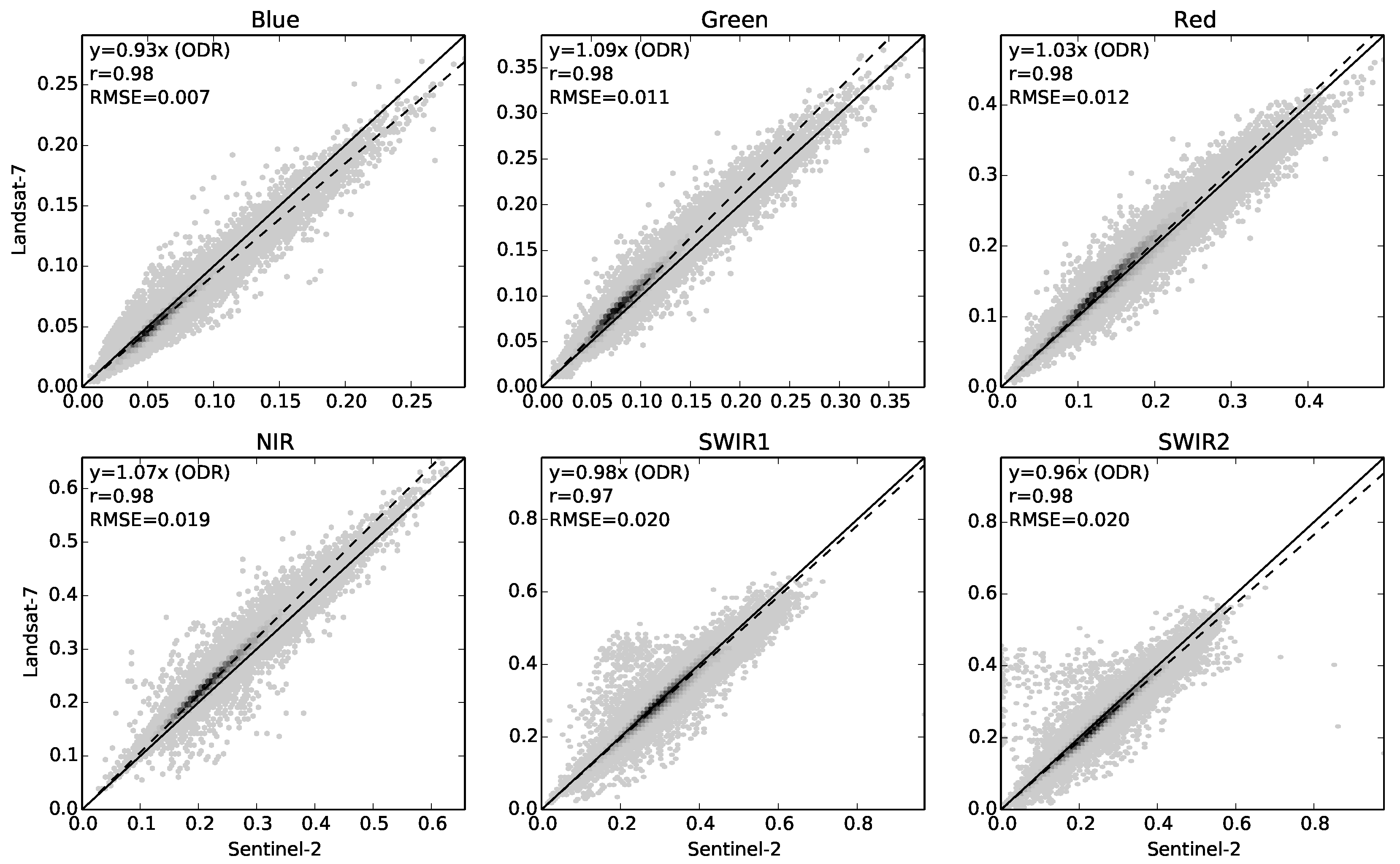
Figure 3.
Comparison of surface reflectance from Sentinel-2A and Landsat-8, for same-day acquisitions. Darker regions represent larger numbers of points. Solid line is 1-to-1, dashed line is the ODR regression fit showing proportional bias.
Figure 3.
Comparison of surface reflectance from Sentinel-2A and Landsat-8, for same-day acquisitions. Darker regions represent larger numbers of points. Solid line is 1-to-1, dashed line is the ODR regression fit showing proportional bias.
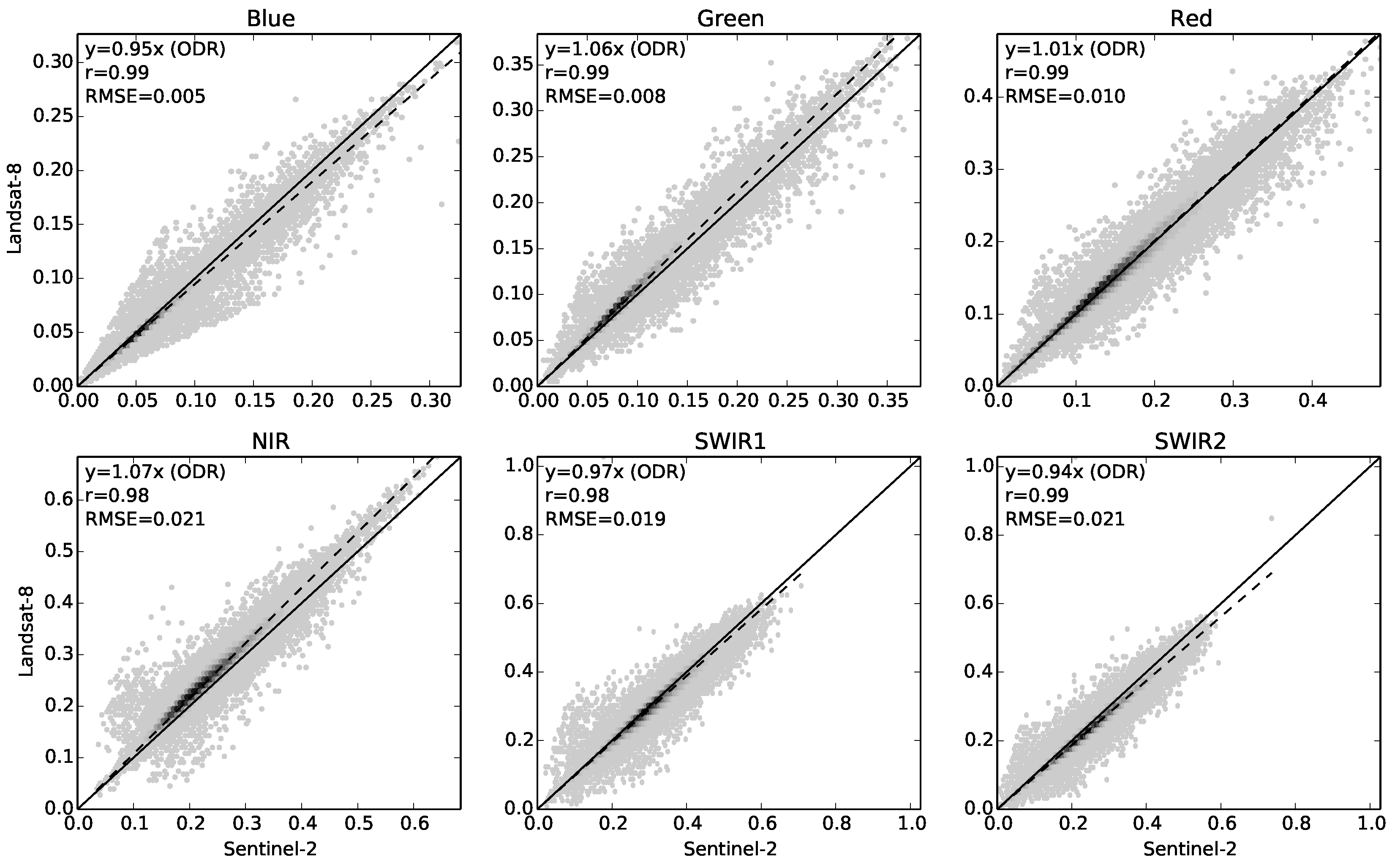
Figure 4.
Comparison of surface reflectance from Sentinel-2A and Landsat-7, for same-day acquisitions after adjusting Sentinel-2A to estimate Landsat-7, using Equation (1). Darker regions represent larger numbers of points. Solid line is 1-to-1, dashed line is the ODR regression fit showing proportional bias.
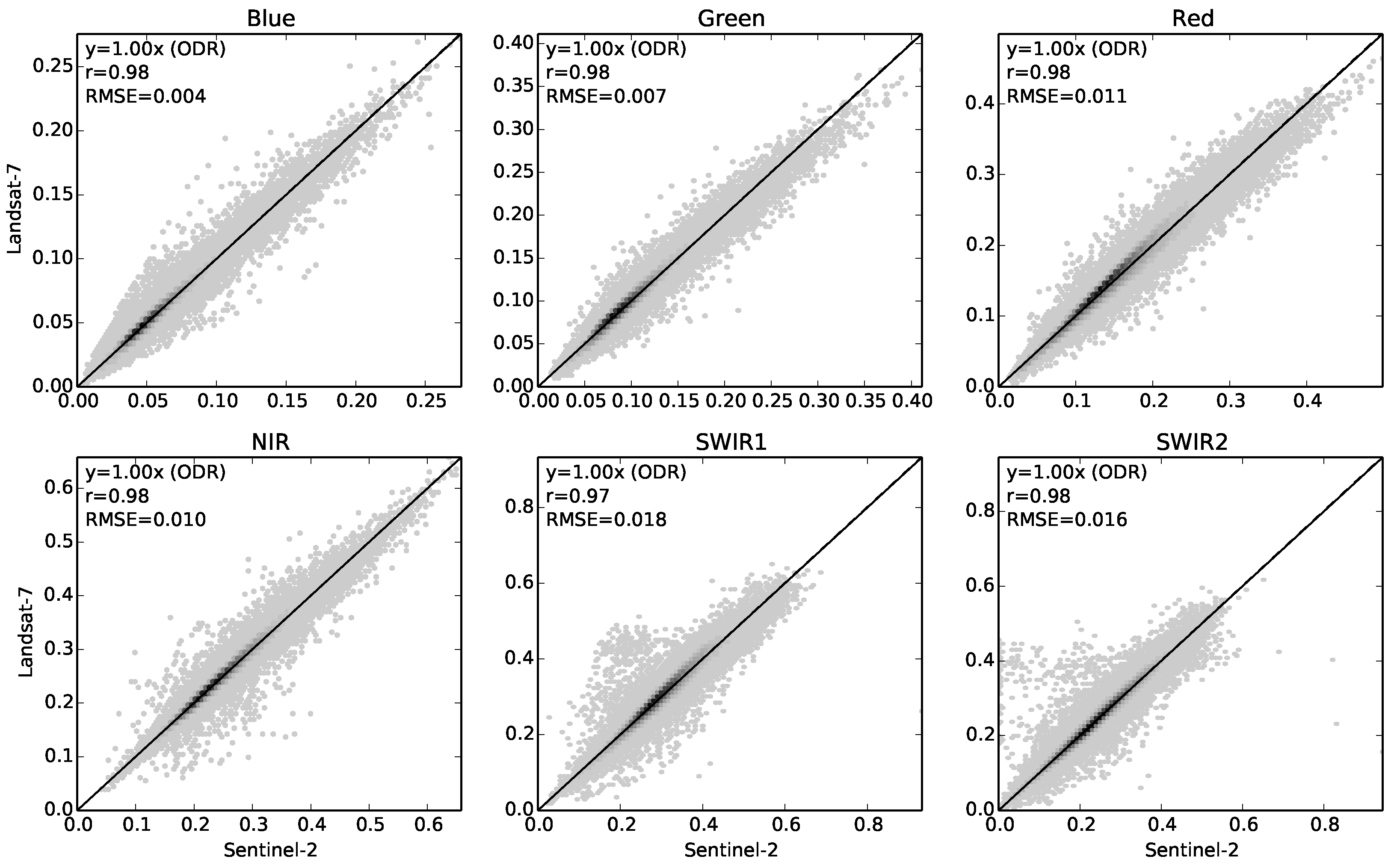
Figure 5.
Comparison of surface reflectance from Sentinel-2A and Landsat-8, for same-day acquisitions after adjusting Sentinel-2A to estimate Landsat-8, using Equation (1). Darker regions represent larger numbers of points. Solid line is 1-to-1, dashed line is the ODR regression fit showing proportional bias.

Figure 6.
Comparison of fractional vegetation cover from Sentinel-2A and Landsat-8, for same-day acquisitions. Darker regions represent larger numbers of points. Solid line is 1-to-1, dashed line is the ODR regression fit showing proportional bias.
Figure 6.
Comparison of fractional vegetation cover from Sentinel-2A and Landsat-8, for same-day acquisitions. Darker regions represent larger numbers of points. Solid line is 1-to-1, dashed line is the ODR regression fit showing proportional bias.
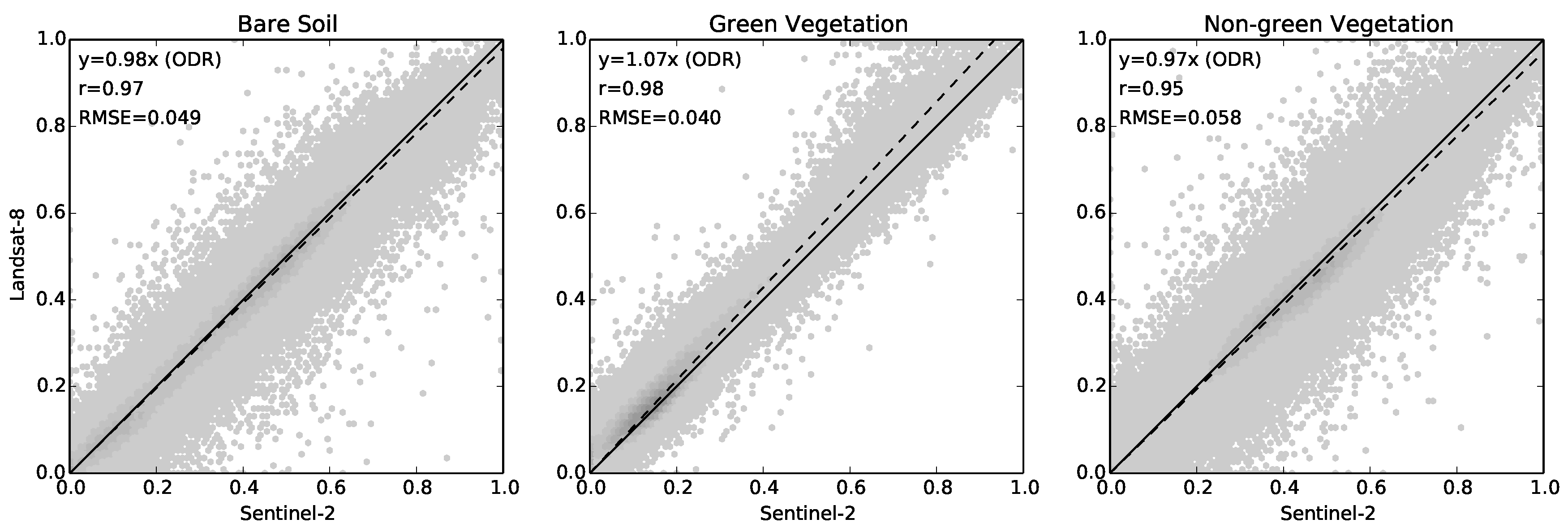
Figure 7.
Comparison of fractional vegetation cover from Sentinel-2A and Landsat-8, for same-day acquisitions, after adjusting Sentinel-2A reflectances to estimate Landsat-8, using Equation (1). Darker regions represent larger numbers of points. Solid line is 1-to-1, dashed line is the ODR regression fit showing proportional bias.
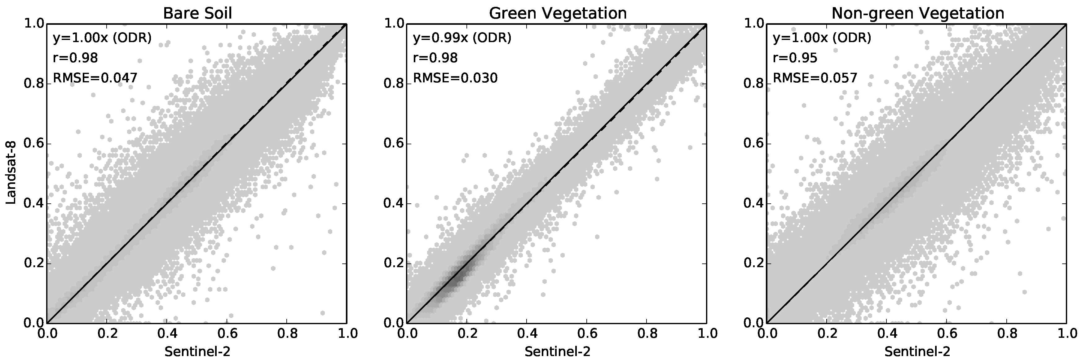
Figure 8.
Comparison of Normalized Difference Vegetation Index (NDVI) from Sentinel-2A and Landsat-8, for same-day acquisitions. (a) using unadjusted surface reflectance; (b) using Sentinel-2A surface reflectance adjusted with Equation (1). Darker regions represent larger numbers of points. Solid line is 1-to-1; dashed line is the ODR regression fit showing proportional bias.

Figure 9.
Comparison of surface reflectance from Sentinel-2A and Landsat-8, for same-day acquisitions after adjusting Sentinel-2A to estimate Landsat-8, using NASA’s HLS adjustment. Darker regions represent larger numbers of points. Solid line is 1-to-1, dashed line is the ODR regression fit. The plot for the NIR band is marked as “Not Applicable” because of the HLS choice of Sentinel-2 band 8A for their NIR band.

Table 1.
Corresponding band numbers for each sensor. Nominal spectral window bounds are included in parentheses (in nanometres).
Table 1.
Corresponding band numbers for each sensor. Nominal spectral window bounds are included in parentheses (in nanometres).
| Generic Name | Sentinel-2 | Landsat-7 | Landsat-8 |
|---|---|---|---|
| Blue | 2 (458–522) | 1 (450–520) | 2 (450–510) |
| Green | 3 (543–578) | 2 (520–600) | 3 (530–590) |
| Red | 4 (650–680) | 3 (630–690) | 4 (640–670) |
| Near Infra-Red (NIR) | 8 (785–900) | 4 (770–900) | 5 (850–880) |
| Short Wave Infra-Red 1 (SWIR1) | 11 (1565–1655) | 5 (1550–1750) | 6 (1570–1650) |
| Short Wave Infra-Red 2 (SWIR2) | 12 (2100–2280) | 7 (2090–2350) | 7 (2110–2290) |
Table 2.
Coefficients for NASA’s Harmonized Landsat-8 Sentinel-2 (HLS) product, to adjust Sentinel-2A reflectance to Landsat-8 reflectance. These are applied in an equation identical to Equation (1). Reproduced here from Claverie et al. [6].
| Coefficient | Blue | Green | Red | NIR | SWIR1 | SWIR2 |
|---|---|---|---|---|---|---|
| 0.00447 | 0.00109 | −0.00104 | 0.000250 | 0.000124 | 0.00119 | |
| 1.020 | 0.994 | 1.017 | 0.999 | 0.999 | 1.003 |
Table 3.
Number of points (single 30 m pixels) used for training and validation, for Landsat-7 and Landsat-8 comparisons.
Table 3.
Number of points (single 30 m pixels) used for training and validation, for Landsat-7 and Landsat-8 comparisons.
| Sensor | Training | Validation |
|---|---|---|
| Landsat-7 | 625,291 | 312,361 |
| Landsat-8 | 610,449 | 304,456 |
Table 4.
Coefficients for Equation (1), to adjust Sentinel-2A reflectance to the corresponding Landsat reflectance. Fitted from the training data described in Table 3.
| Coefficient | Blue | Green | Red | NIR | SWIR1 | SWIR2 | |
|---|---|---|---|---|---|---|---|
| Landsat-7 | −0.0022 | 0.0031 | 0.0064 | 0.012 | 0.0079 | −0.0042 | |
| 0.9551 | 1.0582 | 0.9871 | 1.0187 | 0.9528 | 0.9688 | ||
| Landsat-8 | −0.0012 | 0.0013 | 0.0027 | 0.0147 | 0.0025 | −0.0011 | |
| 0.963 | 1.0473 | 0.9895 | 1.0129 | 0.9626 | 0.9392 |
© 2017 by the author. Licensee MDPI, Basel, Switzerland. This article is an open access article distributed under the terms and conditions of the Creative Commons Attribution (CC BY) license (http://creativecommons.org/licenses/by/4.0/).
Share and Cite
MDPI and ACS Style
Flood, N. Comparing Sentinel-2A and Landsat 7 and 8 Using Surface Reflectance over Australia. Remote Sens. 2017, 9, 659. https://doi.org/10.3390/rs9070659
AMA Style
Flood N. Comparing Sentinel-2A and Landsat 7 and 8 Using Surface Reflectance over Australia. Remote Sensing. 2017; 9(7):659. https://doi.org/10.3390/rs9070659
Chicago/Turabian StyleFlood, Neil. 2017. "Comparing Sentinel-2A and Landsat 7 and 8 Using Surface Reflectance over Australia" Remote Sensing 9, no. 7: 659. https://doi.org/10.3390/rs9070659
Note that from the first issue of 2016, this journal uses article numbers instead of page numbers. See further details here.