Article

Satellite-Based Inversion and Field Validation of Autotrophic and Heterotrophic Respiration in an Alpine Meadow on the Tibetan Plateau

1
Lhasa Plateau Ecosystem Research Station, Key Laboratory of Ecosystem Network Observation and Modeling, Institute of Geographic Sciences and Natural Resources Research, Chinese Academy of Sciences, Beijing 100101, China
2
University of Chinese Academy of Sciences, Beijing 100049, China
3
Institute for Agro-Environmental Sciences, National Agriculture and Food Research Organization, 3-1-3 Kannondai, Tsukuba, Ibaraki 305-8604, Japan
4
College of Global Change and Earth System Sciences, Beijing Normal University, Beijing 100875, China
5
College of Resources and Environment, University of Chinese Academy of Sciences, Beijing 100190, China
*
Author to whom correspondence should be addressed.
Remote Sens. 2017, 9(6), 615; https://doi.org/10.3390/rs9060615
Submission received: 9 May 2017 / Revised: 30 May 2017 / Accepted: 13 June 2017 / Published: 15 June 2017

Abstract

:
Alpine meadow ecosystem is among the highest soil carbon density and the most sensitive ecosystem to climate change. Partitioning autotrophic (Ra) and heterotrophic components (Rm) of ecosystem respiration (Re) is critical to evaluating climate change effects on ecosystem carbon cycling. Here we introduce a satellite-based method, combining MODerate resolution Imaging Spectroradiometer (MODIS) products, eddy covariance (EC) and chamber-based Re components measurements, for estimating carbon dynamics and partitioning of Re from 2009 to 2011 in a typical alpine meadow on the Tibetan Plateau. Six satellite-based gross primary production (GPP) models were employed and compared with GPP_EC, all of which appeared to well explain the temporal GPP_EC trends. However, MODIS versions 6 GPP product (GPP_MOD) and GPP estimation from vegetation photosynthesis model (GPP_VPM) provided the most reliable GPP estimation magnitudes with less than 10% of relative predictive error (RPE) compared to GPP_EC. Thus, they together with MODIS products and GPP_EC were used to estimate Re using the satellite-based method. All satellite-based Re estimations generated an alternative estimation of Re_EC with negligible root mean square errors (RMSEs, g C m−2 day−1) either in the growing season (0.12) or not (0.08). Moreover, chamber-based Re measurements showed that autotrophic contributions to Re (Ra/Re) could be effectively reflected by all these three satellite-based Re partitions. Results showed that the Ra contribution of Re were 27% (10–48%), 43% (22–59%) and 56% (33–76%) from 2009 to 2011, respectively, of which inter-annual variation is mainly attributed to soil water dynamics. This study showed annual temperature sensitivity of Ra (Q10,Ra) with an average of 5.20 was significantly higher than that of Q10,Rm (1.50), and also the inter-annual variation of Q10,Ra (4.14–7.31) was larger than Q10,Rm (1.42–1.60). Therefore, our results suggest that the response of Ra to temperature change is stronger than that of Rm in this alpine meadow.

Graphical Abstract

1. Introduction

Gross primary production (GPP) is plant-driven carbon captures from atmosphere, and thus abundant organic carbon stores in the natural ecosystems [1,2], which forms the basis of all biosphere functions [3]. After GPP, ecosystem respiration (Re) is the second main carbon flux between ecosystems and the atmosphere [4], whose two components, autotrophic and heterotrophic respiration (Ra and Rm), may be controlled in different ways by abiotic and biotic factor [5,6]. For example, response of Ra and Rm to temperature may exhibit different temperature sensitivity (Q10) [7], which is the key parameter of the climate–carbon feedback, usually expressed as the percentage of Re increase for a 10 °C rise in temperature [8]. Climate–carbon feedback depends on whether Rm increases to warming are offset by corresponding increases in GPP [9]. This urges us to give a better understanding of the relative contribution of Ra and Rm components [10]. Recent studies have suggested that the contribution of Ra or Rm is approximately 0.5 [11,12]. However, the average estimates generally mask considerable uncertainties arising from different ecosystems, estimating techniques and time scales [5]. Therefore, accurate quantification of GPP and Re, and, further, effectively partitioning the components of Re, is critical to evaluating potential influence of climate change, especially warming, on ecosystem carbon cycling.
Alpine meadow ecosystems, with about 11.3 Pg of the soil carbon pool in China, is among the ecosystem with the highest soil carbon density (18.2 Kg m−2) [13,14]. In addition, it is one of the most sensitive ecosystems to climate change across the globe [15]. This ecosystem occurs on the Qinghai-Tibetan Plateau, a unique geography mostly situated at 3000 m above sea level, and covers the largest areas (approximately 1/5) of alpine grass ecosystems (2.5 × 10⁶ km2) in this Plateau [16]. Climatic prediction suggests a more intensive climate change, about twice of the average observed global warming rate (increase 0.2 °C per decade) [17], is ongoing on the Tibetan Plateau [15,18]. With its widespread areas and more intense climate change, a clearer understanding of climate–carbon cycle processes on this special ecosystem is necessary for it to serve as a sensitive indicator of regional and global carbon cycles [19,20].
Eddy covariance (EC) is a state-of-the-art method to measure net ecosystem CO2 exchange (NEE) between atmosphere and terrestrial ecosystems [21,22]. Further improvement of regional and global FLUXNET data benefits the needed GPP and Re estimations in EC-based NEE partitions [23,24]. Indeed, EC-based carbon cycle studies increasingly focus on the alpine meadow ecosystem. However, their results are spatially heterogeneous even in evaluating the carbon budgets in this specific ecosystem, which has showed carbon sink [6,14,19,25], carbon neutral [26], or carbon source [27]. Thus, accurate spatial extrapolation from site-specific footprints to regional and global scales is full of challenges.
Satellite-based products provide another pathway to capture quasi-continuous observations of vegetation structure and the resultant GPP estimations across broad temporal and spatial scales [2,28,29,30]. For example, six satellite-based GPP models, MODIS GPP version 5 [31] and 6 products (GPP_MOD5 and GPP_MOD) [32], revised GPP_MOD (GPP_MODR) [33], vegetation photosynthesis model (VPM) [28,29], photosynthetic capacity model (PCM) [34], and the alpine vegetation model (AVM) [35], were widely used to estimate GPP at local, regional, and global scales [30,36]. In general, key parameter inputs of these models, such as the maximum light use efficiency (LUE) [28,29,31,32] or the conversion coefficient [34,35], and the performance of these models are site-specific [30,33,37,38,39,40]. Thus, site-specific ground measurements, especially EC-based measurements, are always required to validate these models and obtain the best satellite-based GPP estimation models in diverse ecosystems. However, Re is rarely quantified from satellite-based products because its soil contribution (Rs) is arduous to observe by remote satellite [41,42]. Recently, using the coupled relationships between Ra and GPP [43], and between Rm and temperature [44], satellite-based models can give us comparable estimations to Re_EC [42]. Nevertheless, another challenge of current EC-based measurements is that they still cannot directly provide partitioning of Ra and Rm components of Re. Thus, no evidence is provided for separately validating the accuracy of Ra and Rm estimations in this alpine meadow.
Chamber-based Re components measurements using gradual plant exclusion can provided complete Re estimations, including Re, Rs, Ra and Rm for site-specific ecosystem [45,46,47,48]. Although recent studies have found chamber-based CO2 measurement generally overestimates or underestimates EC-based measurements [49,50,51], for many ecosystems, the ratios between Re components are similar as measured at specific sites [11,51]. Therefore, in this study, a combination of three methods, EC-based measurements, and satellite- and chamber-based ecosystem carbon flux measurements, were developed in a typical alpine meadow on the central Tibetan Plateau during 2009 to 2011 (Figure 1). Our study objectives were: (1) to select the most instrumental satellite-based GPP estimation methods through multi-model comparison with the EC-based GPP estimations; (2) to introduce a solely satellite-based Re estimation and partition method for seasonal Ra (or Rm) contributions of Re (Ra/Re), and validate its accuracy based on the tower- and chamber-based Re components measurements; and (3) to test what controls the seasonal variation of Ra/Re, and whether seasonal response of Ra and Rm to temperature change is identical in this alpine meadow.

2. Materials and Methods

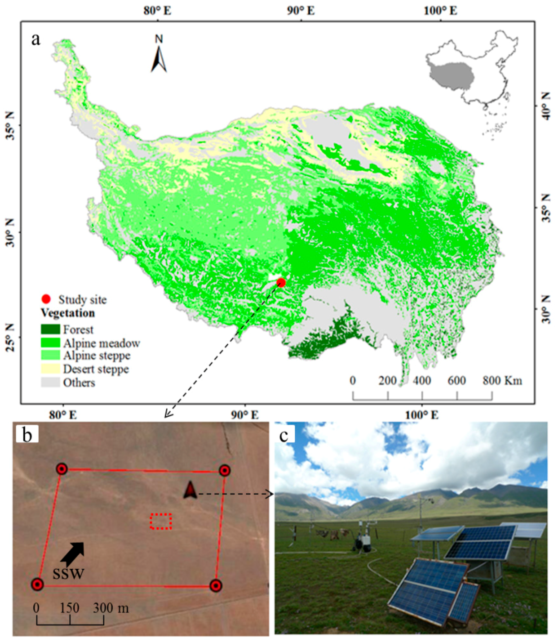
2.1. Site Descriptions

The experimental site is a typical alpine steppe―Korbresia meadow on the northern Tibetan Plateau (30.49783°N, 91.06636°E, elevation 4333 m)—located at the Damxung grassland station, a long-term positioning monitoring station of the Chinese Academy of Sciences (Figure 2). The dominant climate characteristics are strong radiation (annual mean sunlight and solar radiation are 2880.9 h and 7527.6 MJ m−2, respectively), low air temperature, and short cool summers, which is generally categorized as a plateau monsoon climate. Fifty years of climatic records from 1963 to 2012 show that the average annual air temperature is 1.8 °C, with coldest monthly mean of −9.0 °C in January and the warmest of 11.1 °C in July. Average annual precipitation is 476.6 mm, over half of which concentrated in July and August. Flat terrain (less than 2° slope) of this alpine meadow is dominated by three species, Stipa capillacea, Carex montis-everestii and Kobresia pygmaea, the total coverage is about 50–80%. The soil is classified as meadow soil with sandy loam [26] with a shallow soil layer depth of about 30 cm, and the deeper is gravel layer.

2.2. Meteorological, Soil and Vegetation Measurements

The auxiliary meteorological and soil measurements include photosynthetically active radiation (PAR), air temperature at the height of 2 m (Ta), precipitation (PPT), air relative humidity (RHa), vapor pressure deficit (VPD), soil temperature at depths of 5 cm (Ts), and soil water content (SWC). All measurements were averaged and recorded in a data-logger once per 30 min. We also measured the vegetation leaf area index (LAIg) with a harvest method every two weeks during the growing season. From 2009 to 2011, the frozen period (Ts < 0 °C) is from November to March. Vegetation begins to green-up at the beginning of May, thus, in this study, we coarsely defined the growing season from 1 May (the 121st day of year, DOY 121) to mid-October (DOY 281).

2.3. Eddy Covariance-Based Measurements

A standard open-path eddy covariance (EC) system [52] was implemented at the height of 2.1 m in this site to measure net exchange of CO2 (NEE) between atmosphere and vegetation [26]. Due to the occurrence of situations that are inappropriate for EC measurements, including instrument malfunction, rainfall, dew or cobwebs formation, human disturbance, and near-static atmospheric conditions, the EC-based NEE measurements inevitably contain abnormal values [25]. To avoid these potential influences, raw measurements were processed according to the ChinaFLUX data-processing [53,54], which included despiking, coordinate rotation, air density corrections, outlier rejection, and friction velocity threshold (u*) corrections.
The processed data were filled by linear interpolation for small gaps (less than 2 h) in one week window. For gaps more than 2 h, two nonlinear empirical models were applied separately for daytime and nighttime data. The daytime CO2 fluxes were estimated using the Michaelis–Menten equation [55,56].
N E E = a × A m a x × P A R a × P A R + A m a x + R e
where NEE (µmol CO2 m−2 s−1) and Re (µmol CO2 m−2 s−1) are the day time net ecosystem exchange and ecosystem respiration, respectively. Amax (µmol CO2 m−2 s−1) is the maximum ecosystem photosynthesis rate, and α (µmol CO2 µmol photons−1) is the apparent quantum yield. Both are taken as indicators of plant photosynthetic capacity. The nighttime missing NEE data (Re_EC) were filled with the exponential relationship between Re and Ts due to GPP is assumed to be zero at night [57,58].
R e _ E C = a × e ( b × T s )
where Re_EC (µmol CO2 m−2 s−1) is nighttime ecosystem respiration. a (the reference respiration when Ts = 0 °C) and b are the regression parameters, which can be used for daytime Re filled. The gap-filled daytime NEE were partitioned into EC-based GPP (GPP_EC) as CO2 assimilation and Re_EC as CO2 emission during daytime [59].
G P P _ E C = R e _ E C N E E

2.4. Satellite-Based Products

We extracted eight-day MODIS version 6 products, including surface reflectance composite data (MOD09A1, 500 m) [60], land surface temperature (LST) products (MOD11A2, 1 km) [61], MODIS LAI/FPAR data (MOD15A2, 500 m) [62], and MODIS GPP (GPP_MOD) products (MOD17A2, 500 m) [32] at the position of the flux tower for the years 2009 to 2011 from NASA EOSDIS Land Processes Distributed Active Archive Center (LP DAAC, https://lpdaac.usgs.gov/). To compare the agreement between the GPP_MOD and the previous MODIS version 5 GPP products (GPP_MOD5) [31], we also extracted the contemporaneous GPP_MOD5 products (Figure 1).
MODIS GPP products, both GPP_MOD5 and GPP_MOD, were calculated from the MOD17A2 algorithm [31,32] based on light energy use efficiency (LUE) model [2,63].
G P P _ M O D = ε max × f ( Tmin ) × f ( VPD ) × F P A R × S W r a d × 0.45
where εmax (g C MJ−1) is a default parameter obtained from the Biome Properties Look-Up Table (BPLUT), but is not the same for grassland between GPP_MOD5 (0.68 g C MJ−1) and GPP_MOD (0.86 g C MJ−1) [2,31,32,63]. Two attenuation scalars (f(Tmin) and f(VPD)) are simple linear ramp functions of the daily minimum air temperature (Tmin) (Equation (5)) and daytime average VPD (Equation (6)) with a range of 0 to 1 [64]. FPAR is the fraction of absorbed PAR by vegetation canopy that is derived from the MOD15A2 product. Incident shortwave radiation (SWard) are obtained from the NASA Data Assimilation Office (DAO) dataset [65].
f ( T m i n ) = { 0 , T   min T   min _ min T   min _ max T   min _ min , 1 , T   min ( , T   min _ min ] T   min ( T   min _ min , Tmin _ max ) T   min [ T   min _ max , + ) }
f ( V P D ) = { 0 , V P D max V P D V P D max V P D min , 1 , V P D [ V P D max , + V P D ( V P D min , VPDmax ) V P D ( , V P D min ] }
In this alpine meadow, a previous study confirmed GPP_MOD strongly underestimated GPP (about −40.58% of GPP_EC) because of the 16.05% underestimation of εmax and 14.70% overestimation of ground FPAR (FPARg) from 2005 to 2007 [40]. Thus, in this study, we also use the ground observations to revise these two parameter inputs of MOD17A2 algorithm for discussing the accuracy of MODIS products from 2009 to 2011, especially the new GPP_MOD. Based on the Beer–Lambert law [66], FPARg can be calculated from the LAIg measurements (Equation (7)).
F P A R g = 0.95 ( 1 e ( k L A I g ) )
where k is the light extinction coefficient with a value of 0.5 for herbaceous crops in this study [40,67]. The LAIg is a linear regression conversion between ground LAI measurements and MOD15A2 for consecutive measurements on eight-day time step.
εmax can be estimated by three approaches in the growing season. One is the MOD17A2 algorithm based on LAIg and GPP_EC measurement data on LAIg measurement days. More precisely, it is the linear regression slope between GPP_EC and multiple multiplication of f(Tmin), f(VPD), FPARg and PAR on LAIg measurement days [33,40]. The other two approaches are both unit conversion of the apparent quantum yield (α, µmol CO2 µmol photons−1) (Equation (8)) based on the relationship between NEE and PAR [33].
ε max = λ M c α
where λ is the conversion ratio with a value of 4.43 because 1 J energy of PAR is equivalent to 4.43 µmol quantum [68]. Mc (12 g mol1) is the molar quantity of carbon. The difference between these two approaches is the calculation of α, one is based on the Michaelis–Menten rectangular hyperbolic function of NEE and PAR as Equation (1), and the other is based on a linear function between NEE and PAR under low light (PAR < 300 μmol m−2 s−1) [56,69,70]. Thus, in this study, α can be calculated from Equations (9) and (10) [71,72].
a = C a τ C a + 2 τ × a 0
τ = 42.7 + 1.68 × ( T 298 ) + 0.0012 × ( T 298 ) 2
where Ca (μmol mol−1) is the atmospheric CO2 concentration with a value of 350 ppm, α0 (μmol CO2 μmol−1 PAR) is the maximum apparent quantum use efficiency with a value of 0.016 in this study [70], and 𝜏 (μmol mol−1) is the CO2 compensation point, T is the canopy Kelvin temperature (Ta, K).

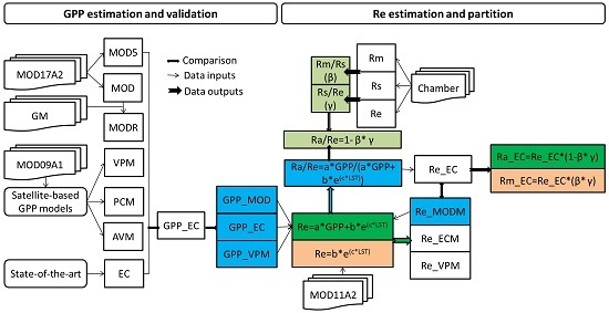
2.5. Satellite-Based GPP Estimations

Satellite-based GPP models can also provide alternative GPP estimations except for the direct MODIS GPP products. In this study, we introduced three satellite-based GPP models, including VPM [28,29,73], PCM [34] and AVM [35], to estimate GPP of this alpine meadow (Figure 1). Both of them are based on the vegetation indices (NDVI and EVI) and land surface water index (LSWI), which can be calculated by Equations (11) to (13) based on the MOD09A1 [29,36,74], respectively. The detailed information for model structures of these three satellite-based GPP models can be completely found in our previous study [30] or separately in their respective references, thus is not repeated here.
N D V I = ρ n i r 1 ρ r e d ρ n i r 1 + ρ r e d
E V I = 2.5 × ( ρ n i r 1 ρ r e d ) ( ρ n i r 1 + 6 × ρ r e d 7.5 × ρ b l u e + 1 )
L S W I = ρ n i r 1 ρ s w i r 1 ρ n i r 1 + ρ s w i r 1
where ρnir1 (841–876 nm), ρred (620–670 nm), ρblue (459–479 nm), and ρswir1 (1628–1652 nm) are the four surface reflectance values from different spectral bands.

2.6. Satellite-Based Re Estimations

Re is mainly composed of two components, autotrophic respiration by plants (Ra) and heterotrophic respiration by heterotrophic microorganisms (Rm) [75]. Ra is the sum of respiration from all plant components, including leaves, stems, flowers of aboveground biomass and roots of underground biomass, which generally depend on current photosynthate [43], and thus couple closely with GPP [42]. Rm is mainly composed of microbial respiration of plant residues and soil organic matter decomposition [43], which is strongly exponentially correlated to temperature variation under water-unlimited conditions [42,44]. Thus in this study, we also considered the LSWI as a water index for regulating the Re variation as Equation (14) [44].
R e = R a + R m = a × G P P + b × e ( c × L S T + d L S W I + e L S W I 2 )
where Re is the satellite-based ecosystem respiration estimations. GPP can be estimated from all the seven methods we mentioned above (Figure 1), and we selected those which have no significant biases for GPP_EC. LST is the land surface temperature that is the average of daytime and nighttime land surface temperature extracted from MOD11A2. a, b, c, d and e are regression parameters. Based on the GPP_EC, we trained the satellite-based Re model separately in growing season (GS) and non-growing season (NG) from 2009 to 2011 (Table 1). In NG, we assumed GPP approaches zero thus we adjusted the parameter of a as zero.
Based on our preliminary test for Equation (14), we found the effect of LSWI on Re estimation was insignificant (p > 0.05) for all separate seasons from 2009 to 2011 (parameters of d and e in Table 1). Therefore, we simplified Equation (14) for further Re estimations (Equation (15)).
R e = R a + R m = a × G P P + b × e ( c × L S T )

2.7. Chamber-Based Re Estimations

Ecosystem respiration (Re) and its components, soil surface CO2 flux (Rs) and Rm, were measured in each polyvinyl chloride (PVC) collar (diameter × height = 20 cm × 5 cm) by a LI-COR 8100 Automated Soil CO2 Flux System (LI-COR Inc., Lincoln, NE, USA) in the growing season from 2010 to 2011. Chamber-based Re measurements are determined by the rate of change of trace gas concentration in the chamber headspace [76,77,78]. We selected 7 sample plots (3 m × 3 m) near the EC flux tower for chamber-based Re measurements, which were basically along the local prevailing wind direction, thus were believed to be similar to the average characteristics of EC-based measurements (Figure 2b). Before the growing season, the PVC collar was randomly inserted into soil at depth of 3–5 cm in each plot for Re and Rs measurements. Re were measured with all plant material in the collar left intact, which includes both above (Ra_above) and belowground components (Rs) (Equation (16)) [45,48].
R e = R s + R a _ a b o v e
After Re measurements, aboveground plant materials within those collars were removed. To avoid the disturbance of clipping and ensure relative steady measurements [12], one day later, we measured Rs, which included Rm and underground autotrophic respiration by plants roots (Ra_under) (Equation (17)) [5,11,43,79].
R s = R m + R a _ u n d e r
Root exclusion was used to estimate Rm, which is the soil CO2 efflux rates without living plant roots respiration [5,47,80]. This alpine meadow had a shallow soil layer depth of about 30 cm, and over 95% of plant roots were contained in the top 0–15 cm of soil layer [47,81]. As the gravel content is high (about 30%) and higher as one goes deeper [26], it is arduous to insert the PVC collars. Thus we selected 4 of 7 measurement plots to develop the root exclusion. The root-free soil quadrat (length × width × height = 0.5 m × 0.5 m × 15 cm) was developed by removing all aboveground and belowground plant materials separately in every 5-cm layer and backfilling the soil according to the original order before the growing season in each plot [47,81]. Then, the PVC collars were inserted into these quadrats to about 13–15 cm depth. These were kept free of plant growth by frequent manual removal during the whole growing season. Rm measurements were identical to Re and Rs measurements [76,77,78].
All chamber-based measurements were conducted with intervals of about 10 days from June to October [48], and each measurement was recorded between 9:00 and 11:00 a.m. for approximating the daily average estimation [82]. Therefore, we can calculate the Ra, the ratio of Rm and Rs (Rm/Rs, β), Rs/Re (γ), Ra/Re (1 − β*γ) based on chamber-based Re (Re_CAM), Rs (Rs_CAM) and Rm measurements (Rm_CAM) as Equations (16) to (20).
R a = R a _ a b o v e + R a _ u n d e r
R m / R s = β R s / R e = γ
R a / R e = 1 β γ

2.8. Components Partitioning of Re

Flux tower was established in a massive and flat alpine steppe—Kobresia meadow—which was over 500 m in all directions. Thus, we confirm that the observation field is homogeneous for our study, which made the comparison between satellite-based and ground measurements feasible. Tower-based CO2 estimations provided consecutive GPP and Re estimations over this alpine meadow. Satellite-based models also supplied eight-day time step GPP and Re estimations, and Re partition for autotrophic and heterotrophic components. Chamber-based Re revealed seasonal variation of the proportion of Re components, which was used to validate the accuracy of the satellite-based Re partition. Thus, using a joint flux tower, satellite-based and chamber-based Re estimations, we separated the EC-based Re estimations into autotrophic (Ra_EC) and heterotrophic components (Rm_EC) based on the calibrated Ra/Re ratio (1 − β*γ) (Figure 1).

2.9. Statistical Analysis

We assumed the plants conditions in each eight-day interval was the same as many previous studies assumed [33,40,42]. Thus, all tower-based flux, meteorological and soil measurements were averaged in eight-day time steps consistent with the remote sensing products. We also put ground vegetation measurements and chamber-based Re estimations into this consecutive eight-day time step measuring series from 2009 to 2011 according to the specific measuring date. We employed linear regression and a paired t-test (α = 0.05) to investigate the performance of different models for GPP estimations as compared to GPP_EC [30]. In addition, two indices, root mean square error (RMSE) and relative predictive error (RPE) (Equations (21) and (22)), were used to evaluate the model agreement and bias from GPP_EC [30,33]. After tests of the normality (Shapiro–Wilk test) and homogeneity of variance (Bartlett test) (p > 0.05), we employed the one-way analysis of variance (ANOVA) and Tukey’s honest significant difference (HSD) to evaluate the accuracy of the cumulative growing season GPP estimations.
R M S E = i = 1 n ( x i y i ) 2 n
R P E = ( y ¯ x ¯ x ¯ ) × 100 %
where xi, x ¯ , yi and y ¯ represents the satellite-based GPP (Re) estimations, the mean value of satellite-based GPP (Re) estimations, the GPP_EC (GPP_Re) time series, and the mean value of GPP_EC (GPP_Re), respectively.
Both those satellite-based GPP estimations that accurately represented GPP_EC (p > 0.05 and RPE < 10%) and GPP_EC were used to evaluate satellite-based Re estimations during the growing season. Satellite-based Re estimations were also compared with the EC-based Re (Re_EC) using identical methods to satellite-based GPP comparison with GPP_EC. The best satellite-based Re estimation was used to partition Re into Ra and Rm. Linear regression and paired t-test (α = 0.05) were used to validate the accuracy of satellite-based Re partition ratios based on the chamber-based Re components measurements. In addition, we test the effect of SWC on seasonal variation of the Re partition ratio, and the missing values of SWC in 2010 were filled by the quadratic regression relationship between SWC and LSWI. Using the exponential relationship between Re and Ts (Equation (2)), we estimated the temperature sensitivity (Q10) of Re and respiration components (Equation (23)) [8].
Q 10 = e ( 10 × b )
where Q10 is used for representing the change in Re and respiration components rate over a 10 °C change in soil temperature, and b is regression parameter from Equation (2). All statistical and modeling procedures were performed in the R statistical computing packages (Version 3.2.0).

3. Results

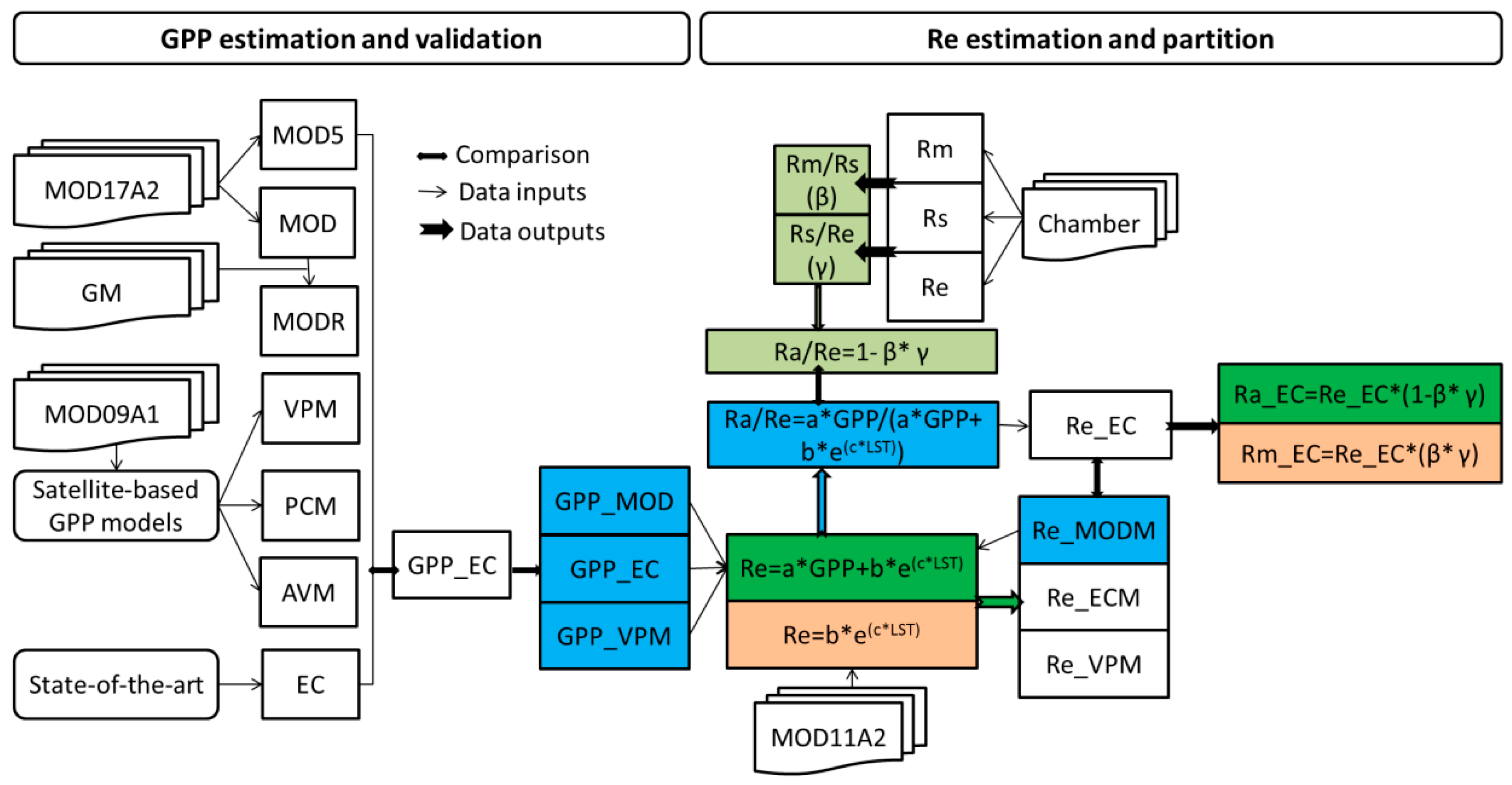
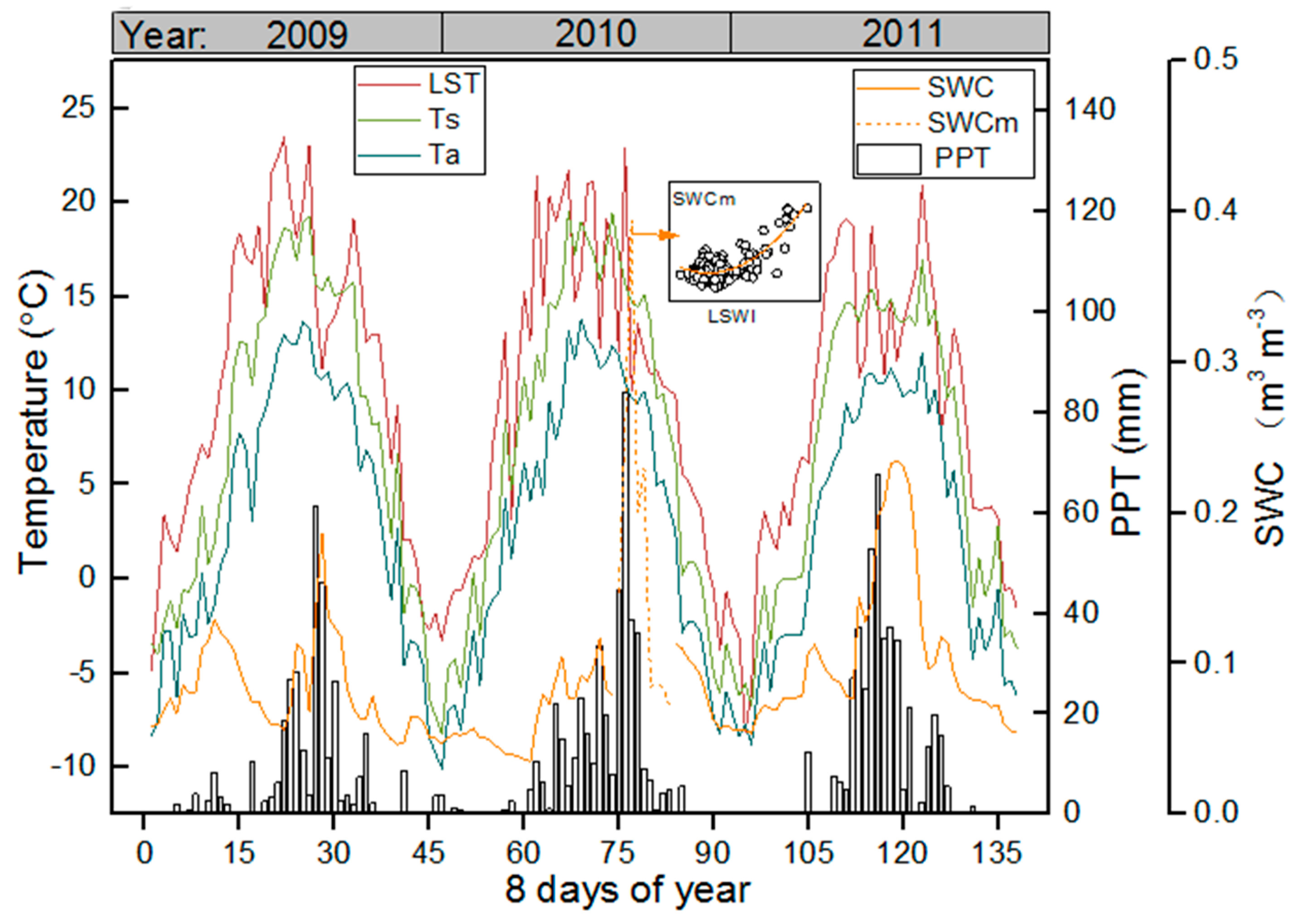
3.1. Meteorological and Vegetation Conditions

Annual average air temperature ranged from 2.3 °C in 2011 to 3.4 °C in 2009 with a mean value of 2.9 °C, which was warmer than 50 year climate records mean (1.8 °C). Soil temperature was generally higher than air temperature by 4.0 °C, and the difference was more pronounced during the growing season (Figure 3). MODIS LST showed a well consistent trend for seasonal and inter-annual temperature variation with ground temperature measurements, but had a significant overestimation of ground temperature measurements. The year 2009 was a drought year with a PPT of 327.7 mm only accounting for 68.7% of 50-year mean rainfall (Figure 3). In general, SWC ranged from 0.05 to 0.25 m3 m−3, except for the higher value (0.39) in 2010 caused by a consecutive 10 days from 17 to 26 August of strong rainfall (daily average of 12.7 mm) (Figure 3).
Two vegetation indices, NDVI and EVI, and the water index, LSWI, had a consistent single peak trend with the peak value generally showing in mid-August (Figure 4a). In contrast, 2009 had a lower growing season NDVI with a mean value of 0.12 and LSWI (0.06) than the latter two years. Seasonal PAR was robust and ranged from 7.5 to 12.5 MJ m−2 day−1 with an average value of 9.83 (±1.81, 1 time standard deviation (SD)) in GS and from 5.8 to 7.5 MJ m−2 day−1 with an average value of 7.45 (±1.83) in NG (Figure 4b). Seasonal PAR reached the peak (about 12.0 MJ m−2 day−1) in the beginning of July, while the maximum FPAR was generally in August, which closely followed the vegetation conditions (Figure 4b). The MODIS FPAR products underestimated the FPARg, which was derived from ground LAI measurements based on the Beer–Lambert law (Equation (7)), in this alpine meadow by a multi-year average of 32.6% in GS except a few days in the beginning of GS (Figure 4b). Seasonal average of FPARg was higher in the final two years (30.3%) than 2009 (25.6%).
A combination of three methods, MOD17A2 algorithm, Michaelis–Menten rectangular hyperbolic function (Equations (1) and (8)), and empirical equation (Equations (8–10)), were used to estimate the εmax values, which were 0.73, 0.73 and 0.75 g C MJ−1 from 2009 to 2011, respectively. Compared to the default value (0.68 g C MJ−1) for grassland in MODIS GPP version 5 (GPP_MOD5), it was underestimated. However, MODIS GPP version 6 (GPP_MOD) used a higher default value of 0.86 g C MJ−1 thus it was overestimated.

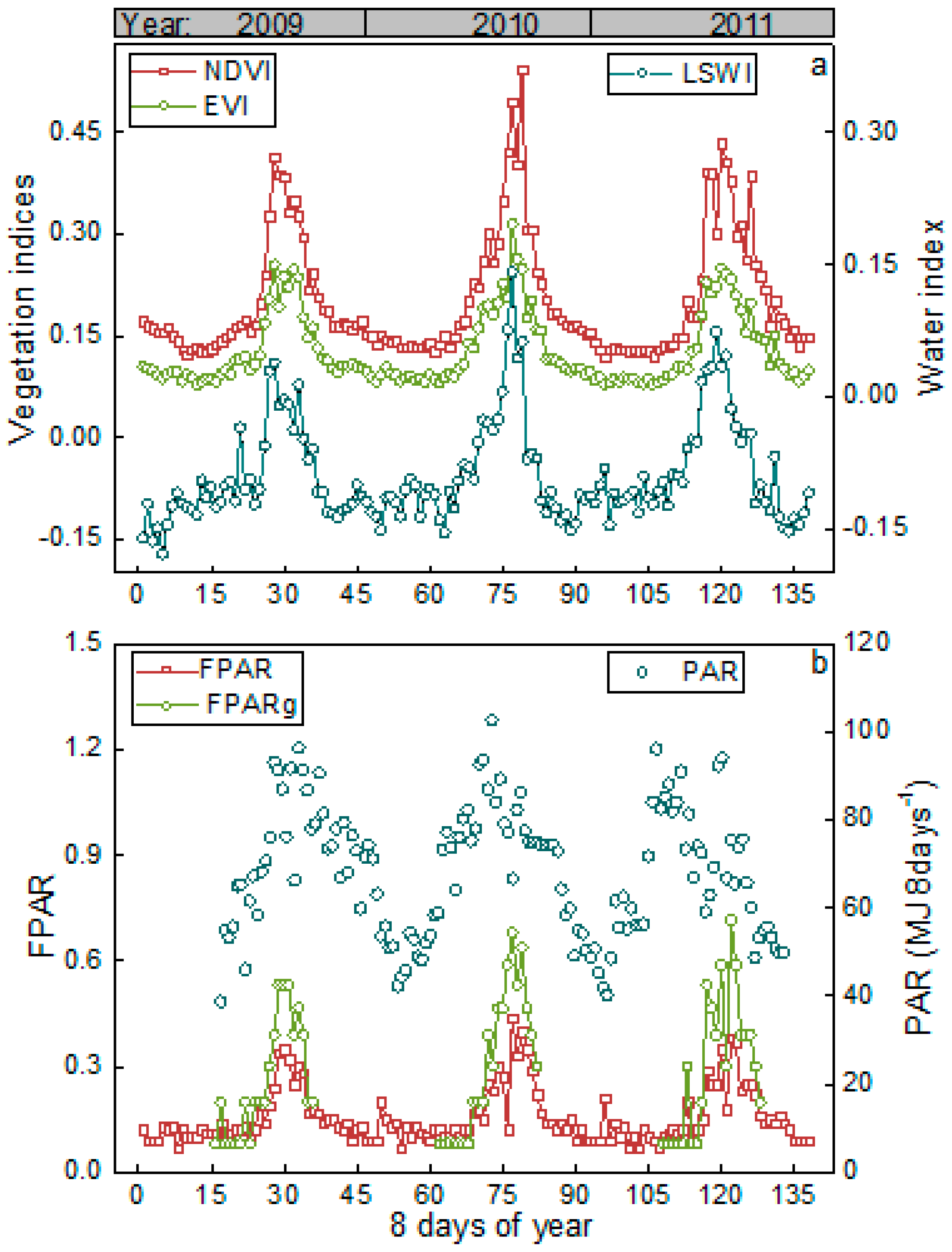
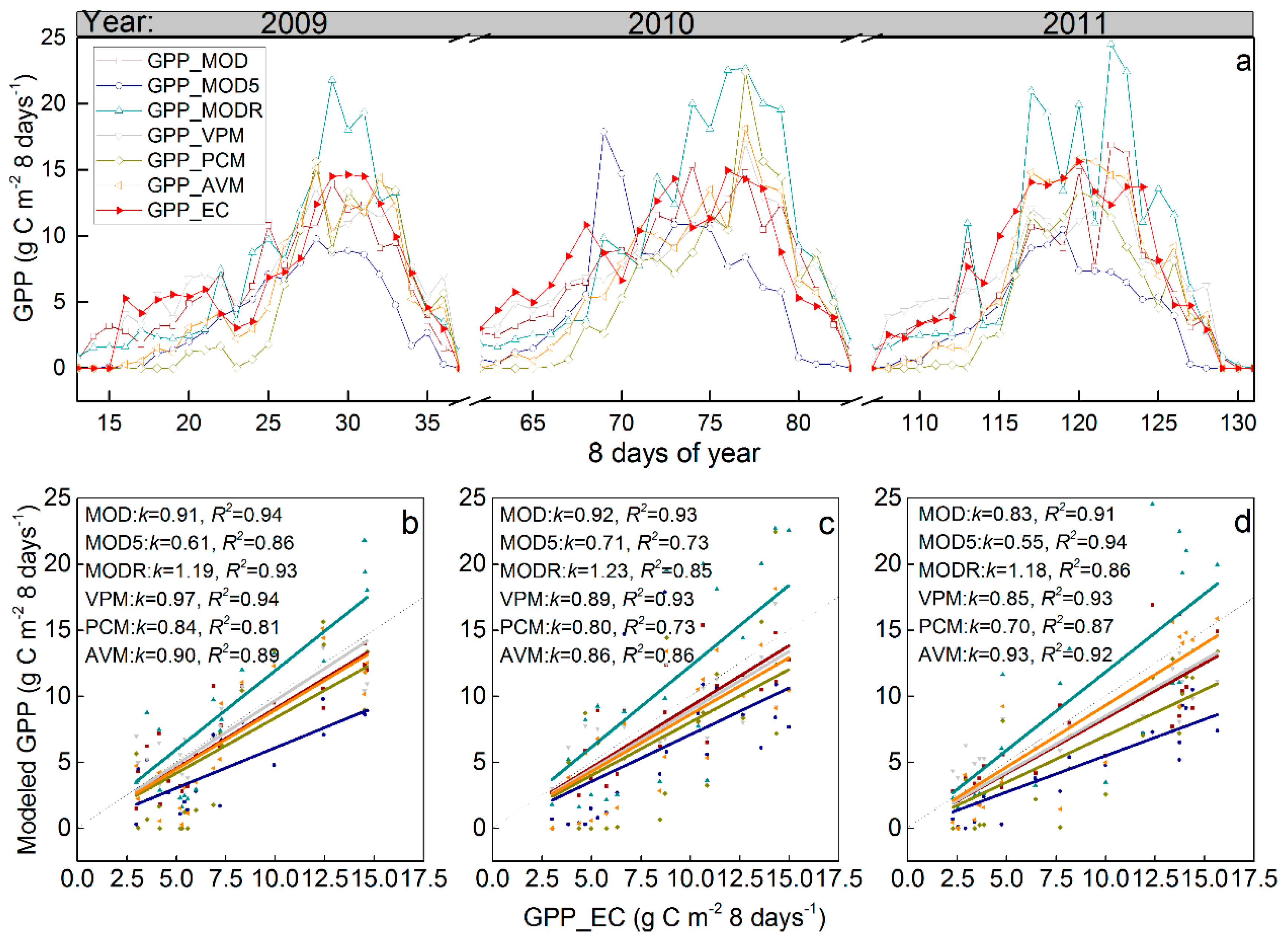
3.2. Satellite-Based GPP Estimations

Six satellite-based GPP estimations (MOD5, MOD, MODR, VPM, PCM and AVM) in this study showed similar seasonal tendencies of GPP_EC but with different quantities in all growing seasons (Figure 5a). Indeed, all these modeled GPP showed an extremely significant (p < 0.0001) linear relationship with EC measurements. This indicates that temporal variation of GPP could be well explained by these satellite-based GPP results (Figure 5b–d). However, different models generally had different performance in accuracy of GPP estimations. For example, MODR had slope (k value in Figure 5b–d) beyond 1.0 in all years, which indicates that MODR overestimated GPP_EC by 18% to 23%. On the contrary, GPP_EC was generally undervalued by the other satellite-based models. In contrast, MOD and VPM not only had the slope most closely approximating to 1.0, from 0.85 to 0.97 for VPM and from 0.83 to 0.92 for MOD, but the best representative of GPP_EC (R2 > 0.9, p < 0.0001) (Figure 5).
Daily average GPP_EC in GS were 0.94, 1.09 and 1.09 g C m−2 day−1 from 2009 to 2011 in this alpine meadow, respectively. MOD5 and PCM strongly underestimated this daily GPP_EC (39.2% and 28.2% of RPE, respectively) with large RMSE values of more than 0.5 g C m−2 day−1 (Table 2). Although the rest of the satellite-based GPP models failed to generate significant deviations for GPP estimation compared to GPP_EC (p > 0.05), they either slightly overestimated (only MODR with 15.9 of RPE), or underestimated, including MOD, AVM, and VPM, the GPP_EC (Figure 5 and Table 2). Specifically, AVM had a 14.5% underestimation for GPP_EC with a RMSE of 0.37 g C m−2 day−1. MOD and VPM further improved the accuracy of GPP estimation by 5.5% of RPE and 11.7% of RPE compared to AVM, which caused smaller RPEs less than 10% with the lowest average RMSE values of 0.31 and 0.32 g C m−2 day−1, respectively (Table 2).
Annual cumulative GPP_EC were 158.09, 183.95 and 183.51 g C m−2 from 2009 to 2011, which were significantly underestimated by MOD5 and PCM with more than 50 g C m−2 of RMSE (Table 2). On the contrary, MODR had a significant (p < 0.05) overestimation for annual cumulative GPP_EC with mean RMSE of 28.43 g C m−2. AVM could be treated as an alternative method to evaluate annual GPP because of the insignificant differences compared to annual GPP_EC, actually, the magnitude of RMSE (25.86 g C m−2) was larger than MOD (17.43 g C m−2) and VPM (10.81 g C m−2) (Table 2). Therefore, VPM and MOD presented superior performances in daily and annual GPP estimations compared to other satellite-based GPP models.

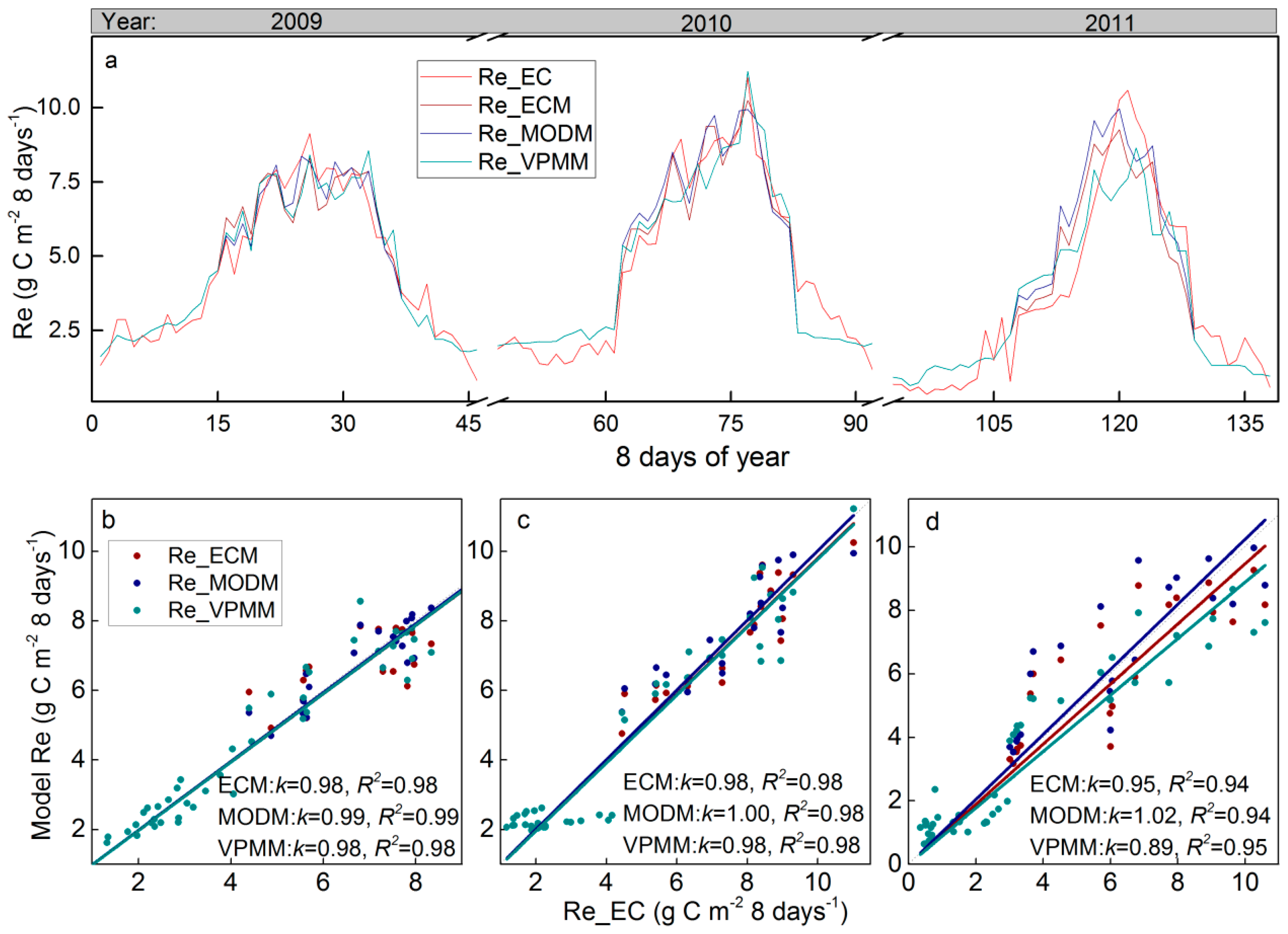
3.3. Satellite-Based Re estimations

We used the most instrumental satellite-based GPP estimation methods, GPP_VPM and GPP_MOD, as compared to GPP_EC and GPP_EC together with MOD11A2 LST products to estimate Re and its components (Ra and Rm) recorded as VPMM, MODM and ECM, respectively (Equation (15) and Figure 1). The temporal variation of Re_EC could be well explained by these three modeled Re values (R2 > 0.9, p < 0.0001) (Figure 6). In addition, the slopes of the linear regression between Re_EC and modeled Re estimations are quite close to 1.0 (mostly from 0.98 to 1.02) (Figure 6b–d), which indicated Re_EC could be effectively estimated by modeled Re estimations.
Daily Re_EC were 0.86, 0.93 and 0.77 g C m−2 in GS and 0.33, 0.28 and 0.17 g C m−2 in NG from 2009 to 2011 (Table 3). All satellite-based daily Re estimations had a small RMSE less than 0.12 g C m−2 day−1 in GS and 0.08 g C m−2 day−1 in NG, which actually did not show significant (p > 0.1) differences compared to Re_EC regardless of in GS or NG (paired t-test, α = 0.05) (Table 3). Thus, both of the cumulative Re estimations in GS and NG calculated from these three satellite-based models also failed to generate significant (p > 0.1) differences with cumulative Re_EC, which showed an average CO2 emission of 143.74 g C m−2 in GS and 51.36 g C m−2 in NG from 2009 to 2011 (Table 3).

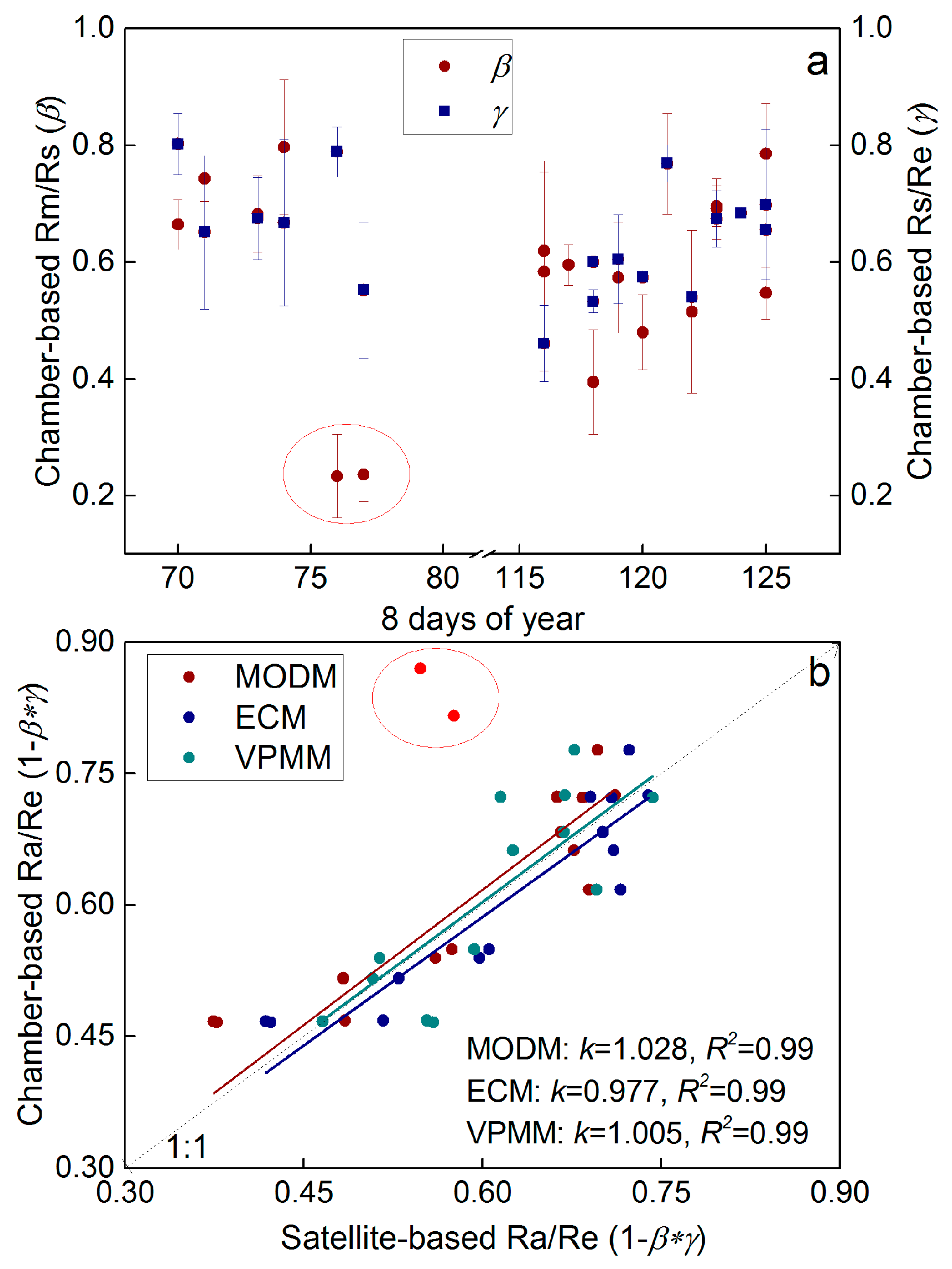
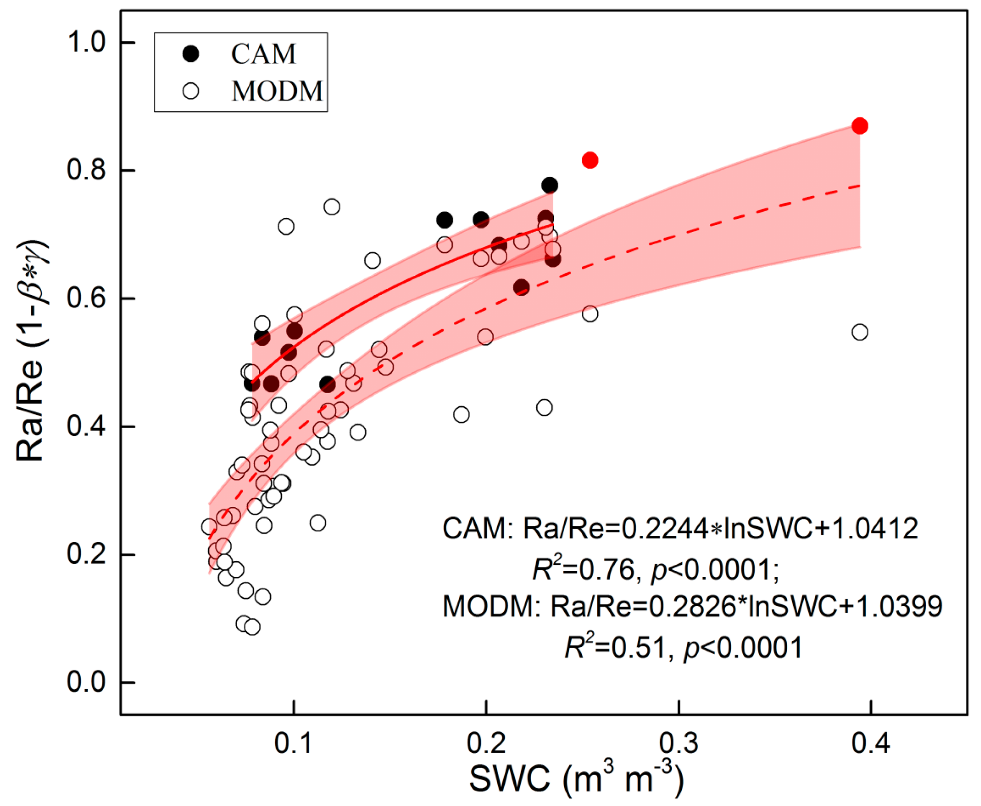
3.4. Re Partitioning and Chamber-Based Validation

We used Re and its components derived from satellite-based VPMM, MODM and ECM to simulate the ratios of Ra and Re (1 − β*γ) (satellite-based Ra/Re), respectively. Meanwhile, chamber-based Re, Rs and Rm measurements directly showed Rm/Rs (β) and Rs/Re (γ), which can also be used to calculate Ra/Re (1 − β*γ) (chamber-based Ra/Re) from 2010 to 2011 (Figure 7). Both satellite-based Ra/Re and chamber-based Ra/Re were not constant throughout the GS. Specifically, all three satellite-based Ra/Re ranged from 0.21 to 0.76 with an average value of 0.50 (±0.14, SD, n = 126) from 2010 to 2011. Chamber-based Re measurements showed that both Rm/Rs and Rs/Re ranged from 0.40 to 0.80 with two exceptions of Rm/Rs that were around 0.20 (dots in circle in Figure 7a). Thus, chamber-based Ra/Re ranged from 0.39 to 0.87, including two values of 0.82 and 0.87 that derived from two abnormal measurements of Rm/Rs (red dots in Figure 6b). Excluding these two abnormal measurements, which will be further discussed later, chamber-based Ra/Re could be well explained (slope ≈ 1.0 from 0.98 to 1.03, R2 = 0.99, p < 0.0001) by all three satellite-based Ra/Re (Figure 7b). In addition, all three satellite-based Ra/Re failed to pose significant differences with chamber-based Ra/Re (paired t-test, α = 0.05, p > 0.1). Therefore, any of Ra/Re from satellite-based models calibrated by corresponding linear relationships with chamber-based Ra/Re can be used to separate the EC-based Re estimations into autotrophic (Ra_EC) and heterotrophic components (Rm_EC).
In this study, we selected MODM because it was the most convenient method whose data inputs, GPP_MOD and LST, can be directly extracted from MODIS products. In the growing season, the average Ra_EC/Re_EC ratios were 0.27 (0.10–0.48, seasonal variation), 0.43 (0.22–0.59) and 0.56 (0.30–0.76) from 2009 to 2011, respectively.

4. Discussion

4.1. Variability of Re Components

Our results showed that Ra/Re (1 − β*γ) was not constant, but with a distinct seasonal variation throughout the growing season in this alpine meadow. The contribution of Ra to Re rises with spring warming and generally reaches the maximum value in the vigorous growth period, then declines with autumn cooling [9,49,78,79,83,84]. Although research on Rs/Re (γ) also showed a distinct seasonal pattern similar to Ra/Re before the summer, this ratio increased again in the following autumn [78,85]. Different trends between the two ratios might ascribe to different controlling mechanisms. Specifically, the Ra/Re was mainly followed plants’ photosynthetic capacity from the phonological stages and was generally coupled with the seasonality of temperature and moisture [9,86]. However, the Rs/Re was mainly controlled by the availability of stored substrates and the lags between temperature changes of air and soil [78]. The heterotrophic contribution to Rs (β) is relatively robust and showed only a negligible seasonal pattern compared to Ra/Re (1 − β*γ) and Rs/Re (γ) [9,81,84,85], because both autotrophic and heterotrophic respiration increased with seasonal warming [9].
In this study, chamber-based Rm/Rs (β) generally ranged from 0.40 to 0.80 with two obvious exceptions around 0.2, which were measured on 24 August and 4 September 2010 (Figure 7a). These two days both had extremely high SWC caused by consecutive strong rainfall events (Figure 3), which dramatically stimulated the autotrophic contribution to Re due to the significantly positive relationship between SWC and Ra/Re (p < 0.0001) (Figure 8). Many relevant studies also suggest that high SWC has a more significant effect on plant activity than on soil microorganisms [84]. Meanwhile, extremely high SWC inhibited Rm from deep soil layers due to the water block of soil porosity [87], and limited the oxygen supply for decomposition by aerobic microbes [88]. Besides, root exclusion was likely to intensify soil moisture due to a decrease of transpiration under this extremely wet condition [12,84]. Although these pulse effects were not detected by satellite-based Ra/Re (Figure 7b), the daily SWC in this semiarid alpine meadow was generally less than 0.25 (Figure 3). In addition, any other chamber-based measuring dates were selected at least two days after a rainfall event [47]. Therefore, to avoid the impacts of pulse effects and ensure the comparability with other chamber-based measurements, these two measurements were assumed to be abnormal and excluded from further analysis.
In the growing season during 2009 to 2011, our results showed that autotrophic contribution to Re (Ra_EC/Re_EC) ranged from 0.27 to 0.56, which fell within the range of similar alpine ecosystem in Qinghai [83] and Tibet [45] (Table 4). However, it was slightly lower than that of an alpine meadows in Haibei [79], which might be mainly caused by the significant lower biomass (91.9 g drought weight (DW) m−2) in this site than Haibei with biomass of 355.7–512.4 g DW m−2 in 2009 [79]. Meanwhile, the inter-annual variation of Ra_EC/Re_EC showed that the year 2009 had a lower autotrophic contribution to Re (Ra_EC/Re_EC) (0.27) than the latter two years (0.50), which attributed to the most drought and lowest vegetation conditions (NDVI) in 2009 (Figure 3, Figure 4 and Figure 8).

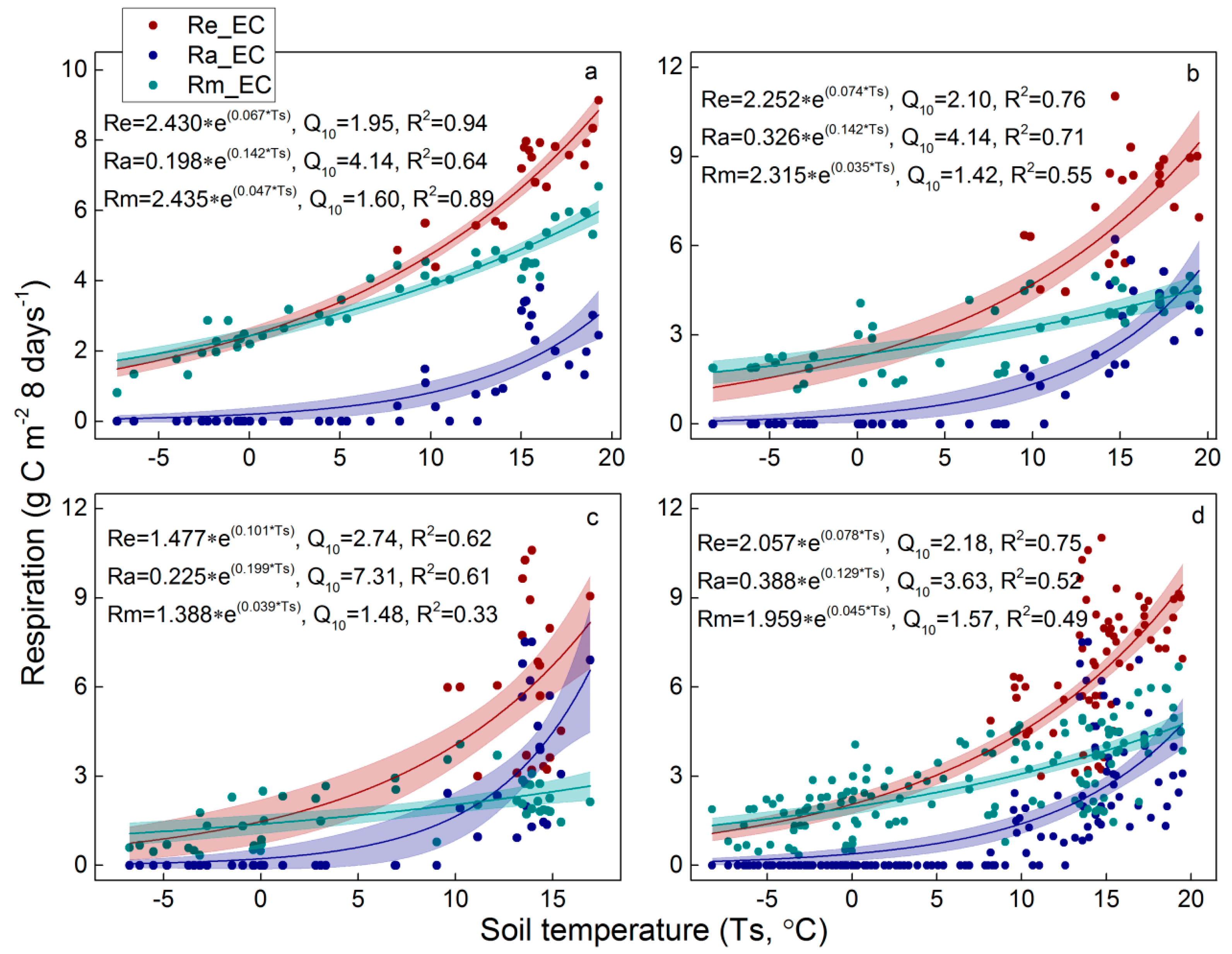
4.2. Temperature Sensitivity of Re Components

Our results showed that temperature sensitivity of Re_EC (Q10,Re) was 2.26, ranging from 1.95 to 2.74 from 2009 to 2011 (Figure 9a–c), which is slightly lower than 2003 (3.2) and 2004 (3.4) in this alpine meadow [26]. For one reason, warmer (about 1 °C) and drier (about 150 mm annual precipitation) climatic conditions played crucial roles for the decreased Q10,Re in this study compared to in 2003 and 2004, which could be evidenced in many relevant studies [89,90,91,92]. Indeed, we also found that the year with cooler and wetter climate showed a greater Q10,Re amid these three years (Figure 8). For another reason, the higher Q10,Re was estimated only during the GS of 2003 and 2004, while we estimated Q10,Re in this study based on annual scale. Thus, the vegetation seasonality or the different contributions of Ra to Re was likely to exert important impacts on Q10,Re variation [93,94].
After partitioning of Re components at seasonal scale, we found that temperature sensitivity of Ra_EC (Q10,Ra) with an average of 5.20 was significantly higher than that of Rm_EC with an average of 1.50 (Q10,Rm) (Figure 9). Our results confirmed that autotrophic and heterotrophic contributions of Re differed in their responses to temperature change [94,95]. Furthermore, variation of Q10 in Rm (1.42 to 1.60) was more stable than that in Ra (4.14 to 7.31) (Figure 9a–c), which implying that the ecosystem acclimation of Ra might be stronger than heterotrophic contributions of Re response to temperature change [95,96,97].

4.3. Methods Applications and Uncertainty

In this study, we provided a pure satellite-based method, which was driven by MODIS GPP and LST products, to estimate and partition Re, and we confirmed it could generate comparable results by validation and improvement from tower- and chamber-based measurements. High temporal-spatial resolution of remote sensing products give the method two potential applications. The direct application is to estimate and partition Re into autotrophic and heterotrophic contributions in similar alpine meadows, which would help in accurate quantification of carbon balance under future climate change [11,46,85,95]. Moreover, many parameter inputs used in bulks of biogeochemical cycle models, such as Q10 [98], net ecosystem productivity (NEP, GPP-Ra) and net carbon sequestration (1-Re/GPP) [99], can also be simply estimated.
However, there are some cautions should be taken for further application of this satellite-based Re estimation and partition method. One is that spatial extrapolation for other vegetation types or regions should be based on appropriate validation, such as chamber-based measurements as we have suggested in this study. For example, PCM underestimated GPP at this alpine meadow, but it could be used as an alternative method for GPP estimation, albeit with a bit of overestimation about 10% of GPP_EC, in near alpine swamp meadow [30] and in the ecosystems of northern China [34]. Thus, ground validation is needed for further scale extrapolation.
The other fact is that the satellite-based Re estimation and partition method is not sensitive to pulse effect of rainfall on Re, resulting in underestimation of Ra/Re compared to the chamber-based Re partition. However, this study confirmed that the satellite-based Ra/Re could explain chamber-based Ra/Re without significant discrepancies. For one reason, this kind of instantaneous underestimation would be weakened after reconciling Re measurements at eight-day composited time resolution. For another reason, instantaneous change of components of Rs due to disturbance of rainfall pulse might gradually tend to re-equilibration with recovery of the soil gas-permeability [87]. Thus, chamber-based Re measurements should effectively avoid the rainfall events for stable and representative measurements [47].
The remaining uncertainties are likely to originate from the undemanding agreement of temporal-spatial matching between MODIS-based products and ground measurements [33,100]. Specifically, MODIS products has an regular eight-day time step and 1 km pixel, while chamber-based measurements only reflects the specific Re state in the measurement day and the restricted samples plot we selected, thus the errors of temporal-spatial match is inevitable. However, this mismatch failed to significantly affect the accuracy of GPP and Re estimation, and Re partitioning in this alpine meadow.

5. Conclusions

This study introduced a pure satellite-based method to estimate GPP and Re, and partitioning Re from 2009 to 2011 in one typical alpine meadow on the Tibetan plateau. Using flux-tower measurements and chamber-based Re components measurements, we also validated and discussed its application and uncertainty. Temporal variation of GPP could be well explained by six satellite-based GPP estimations, including GPP_MOD5, GPP_MOD, GPP_MODR, GPP_VPM, GPP_PCM and GPP_AVM. Daily average GPP_EC in GS were 0.94, 1.09 and 1.09 g C m−2 day−1 from 2009 to 2011, respectively. In contrast, GPP_MOD and GPP_VPM provided the most reliable satellite-based GPP estimations (less than 10% of RPE) compared to GPP_EC. Then, using GPP_EC, GPP_MOD and GPP_VPM, together with MODIS products, satellite-based Re estimations, Re_ECM, Re_MODM and Re_VPMM, were compared with the Re_EC. Daily Re_EC were 0.86, 0.93 and 0.77 g C m−2 in GS, and 0.33, 0.28 and 0.17 g C m−2 in NG from 2009 to 2011, respectively. All satellite-based Re estimations could give an alternative estimation of Re_EC with a negligible bias less than 0.12 and 0.08 g C m−2 day−1 of RMSE in GS and NG, respectively. Moreover, chamber-based Re (Re_CAM) partitioning of autotrophic (Ra_CAM) and heterotrophic (Rm_CAM) contributions showed that Ra_CAM/Re_CAM could be effectively reflected by all these three satellite-based Re partitions. Our results showed that 27% (10–48%), 43% (22–59%) and 56% (33–76%) of Re_EC were plant autotrophic respiration (Ra_EC) from 2009 to 2011, respectively, whose inter-annual variation was ascribed to soil water content dynamics. Our results suggested response of seasonal Ra and Rm to temperature change is different. Specifically, the temperature sensitivity of Ra_EC (Q10,Ra) with an average of 5.20 was significantly higher than that of Rm_EC with an average of 1.50 (Q10,Rm), and the inter-annual variation of Q10,Ra (4.14–7.31) also larger than Q10,Rm (1.42–1.60). Thus, this study suggested that response of Ra to temperature change might be stronger than Rm in this alpine meadow, which confirmed that partitioning Re into Ra and Rm facilitates a better understanding of carbon balance in this alpine meadow. High temporal-spatial resolution of remote products made this kind of satellite-based Re estimation and partitioning easy to upscale both at temporal and spatial scale, especially in the remote areas with scarce field observation.

Acknowledgments

We thank the editors and reviewers for their insightful and valuable comments; and Meng Li and Zhipeng Wang for their help in manuscript improvement. This work was supported by the National Natural Science Foundation of China (No. 41571042; Name: Quantitative identification on the influence of climate change and human activities in the alpine meadow ecosystem on the Northern Tibet), the National Key Research and Development Program (No. 2016YFC0502001; Name: Optimized configuration technologies for production and ecological functions on Tibet grassland), and the Strategic Priority Research Program of the Chinese Academy of Sciences (No. XDB03030401; Name: Effect of climate warming on alpine shrub and meadow ecosystem on the Tibetan plateau).

Author Contributions

Ben Niu and Xianzhou Zhang conceived and designed this study. Ben Niu, Yongtao He, Ning Zong and Gang Fu collected and analyzed the data. Xianzhou Zhang, Yongtao He, Peili Shi and Mingyuan Du contributed observation apparatus. Ben Niu wrote the paper with many valuable suggestions from all other co-authors.

Conflicts of Interest

The authors declare no conflict of interest.

References

  1. Beer, C.; Reichstein, M.; Tomelleri, E.; Ciais, P.; Jung, M.; Carvalhais, N.; Rodenbeck, C.; Arain, M.A.; Baldocchi, D.; Bonan, G.B.; et al. Terrestrial gross carbon dioxide uptake: Global distribution and covariation with climate. Science 2010, 329, 834–838. [Google Scholar] [CrossRef] [PubMed]
  2. Running, S.W.; Thornton, P.E.; Nemani, R.; Glassy, J.M. Global terrestrial gross and net primary productivity from the earth observing system. In Methods in Ecosystem Science; Sala, O., Jackson, R., Mooney, H., Howarth, R., Eds.; Springer: New York, NY, USA, 2000; pp. 44–57. [Google Scholar]
  3. Gitelson, A.A.; Viña, A.; Verma, S.B.; Rundquist, D.C.; Arkebauer, T.J.; Keydan, G.; Leavitt, B.; Ciganda, V.; Burba, G.G.; Suyker, A.E. Relationship between gross primary production and chlorophyll content in crops: Implications for the synoptic monitoring of vegetation productivity. J. Geophys. Res. Atmos. 2006, 111. [Google Scholar] [CrossRef]
  4. Chen, B.X.; Zhang, X.Z.; Tao, J.; Wu, J.S.; Wang, J.S.; Shi, P.L.; Zhang, Y.J.; Yu, C.Q. The impact of climate change and anthropogenic activities on alpine grassland over the qinghai-tibet plateau. Agric. For. Meteorol. 2014, 189, 11–18. [Google Scholar] [CrossRef]
  5. Zhou, X.; Wan, S.; Luo, Y. Source components and interannual variability of soil CO2 efflux under experimental warming and clipping in a grassland ecosystem. Glob. Chang. Biol. 2007, 13, 761–775. [Google Scholar]
  6. Kato, T.; Tang, Y.H.; Gu, S.; Hirota, M.; Cui, X.Y.; Du, M.Y.; Li, Y.N.; Zhao, X.Q.; Oikawa, T. Seasonal patterns of gross primary production and ecosystem respiration in an alpine meadow ecosystem on the qinghai-tibetan plateau. J. Geophys. Res. Atmos. 2004, 109. [Google Scholar] [CrossRef]
  7. Rey, A.; Pegoraro, E.; Tedeschi, V.; De Parri, I.; Jarvis, P.G.; Valentini, R. Annual variation in soil respiration and its components in a coppice oak forest in central italy. Glob. Chang. Biol. 2002, 8, 851–866. [Google Scholar] [CrossRef]
  8. Raich, J.W.; Schlesinger, W.H. The global carbon-dioxide flux in soil respiration and its relationship to vegetation and climate. Tellus Ser. B Chem. Phys. Meteorol. 1992, 44, 81–99. [Google Scholar] [CrossRef]
  9. Hicks Pries, C.E.; Schuur, E.A.G.; Crummer, K.G. Thawing permafrost increases old soil and autotrophic respiration in tundra: Partitioning ecosystem respiration using δ13c and ∆14c. Glob. Chang. Biol. 2013, 19, 649–661. [Google Scholar] [CrossRef] [PubMed]
  10. Buchmann, N. Biotic and abiotic factors controlling soil respiration rates in picea abies stands. Soil Biol. Biochem. 2000, 32, 1625–1635. [Google Scholar] [CrossRef]
  11. Bond-Lamberty, B.; Wang, C.; Gower, S.T. A global relationship between the heterotrophic and autotrophic components of soil respiration? Glob. Chang. Biol. 2004, 10, 1756–1766. [Google Scholar] [CrossRef]
  12. Hanson, P.J.; Edwards, N.T.; Garten, C.T.; Andrews, J.A. Separating root and soil microbial contributions to soil respiration: A review of methods and observations. Biogeochemistry 2000, 48, 115–146. [Google Scholar] [CrossRef]
  13. Ni, J. Carbon storage in grasslands of China. J. Arid Environ. 2002, 50, 205–218. [Google Scholar] [CrossRef]
  14. Saito, M.; Kato, T.; Tang, Y. Temperature controls ecosystem CO2 exchange of an alpine meadow on the northeastern tibetan plateau. Glob. Chang. Biol. 2009, 15, 221–228. [Google Scholar] [CrossRef]
  15. Chen, H.; Zhu, Q.; Peng, C.; Wu, N.; Wang, Y.; Fang, X.; Gao, Y.; Zhu, D.; Yang, G.; Tian, J.; et al. The impacts of climate change and human activities on biogeochemical cycles on the qinghai-tibetan plateau. Glob. Chang. Biol. 2013, 19, 2940–2955. [Google Scholar] [CrossRef] [PubMed]
  16. Zheng, D.; Zhang, Q.; Wu, S. Mountain Geoecology and Sustainable Development of the Tibetan Plateau; Springer Science & Business Media: Berlin, Germany, 2000; Volume 57. [Google Scholar]
  17. IPCC—Intergovernmental Panel on Climate Change. Impacts, Adaptation and Vulnerability: Regional Aspects; Cambridge University Press: Cambridge, UK, 2014. [Google Scholar]
  18. Liu, X.; Chen, B. Climatic warming in the tibetan plateau during recent decades. Int. J. Climatol. 2000, 20, 1729–1742. [Google Scholar] [CrossRef]
  19. Zhao, L.; Li, Y.; Xu, S.; Zhou, H.; Gu, S.; Yu, G.; Zhao, X. Diurnal, seasonal and annual variation in net ecosystem CO2 exchange of an alpine shrubland on qinghai-tibetan plateau. Glob. Chang. Biol. 2006, 12, 1940–1953. [Google Scholar] [CrossRef]
  20. Li, J.; Fang, X. Uplift of the tibetan plateau and environmental changes. Chin. Sci. Bull. 1999, 44, 2117–2124. [Google Scholar] [CrossRef]
  21. Vesala, T.; Kljun, N.; Rannik, Ü.; Rinne, J.; Sogachev, A.; Markkanen, T.; Sabelfeld, K.; Foken, T.; Leclerc, M.Y. Flux and concentration footprint modelling: State of the art. Environ. Pollut. 2008, 152, 653–666. [Google Scholar] [CrossRef] [PubMed]
  22. Baldocchi, D.D. Assessing the eddy covariance technique for evaluating carbon dioxide exchange rates of ecosystems: Past, present and future. Glob. Chang. Biol. 2003, 9, 479–492. [Google Scholar] [CrossRef]
  23. Baldocchi, D.; Falge, E.; Gu, L.H.; Olson, R.; Hollinger, D.; Running, S.; Anthoni, P.; Bernhofer, C.; Davis, K.; Evans, R.; et al. Fluxnet: A new tool to study the temporal and spatial variability of ecosystem-scale carbon dioxide, water vapor, and energy flux densities. Bull. Am. Meteorol. Soc. 2001, 82, 2415–2434. [Google Scholar] [CrossRef]
  24. Reichstein, M.; Falge, E.; Baldocchi, D.; Papale, D.; Aubinet, M.; Berbigier, P.; Bernhofer, C.; Buchmann, N.; Gilmanov, T.; Granier, A.; et al. On the separation of net ecosystem exchange into assimilation and ecosystem respiration: Review and improved algorithm. Glob. Chang. Biol. 2005, 11, 1424–1439. [Google Scholar] [CrossRef]
  25. Niu, B.; He, Y.; Zhang, X.; Du, M.; Shi, P.; Sun, W.; Zhang, L. CO2 exchange in an alpine swamp meadow on the central Tibetan Plateau. Wetlands 2017, 37, 525–543. [Google Scholar] [CrossRef]
  26. Shi, P.L.; Sun, X.M.; Xu, L.L.; Zhang, X.Z.; He, Y.T.; Zhang, D.Q.; Yu, G.R. Net ecosystem CO2 exchange and controlling factors in a steppe—Kobresia meadow on the tibetan plateau. Sci. China Ser. D 2006, 49, 207–218. [Google Scholar] [CrossRef]
  27. Zhao, L.; Li, J.; Xu, S.; Zhou, H.; Li, Y.; Gu, S.; Zhao, X. Seasonal variations in carbon dioxide exchange in an alpine wetland meadow on the qinghai-tibetan plateau. Biogeosciences 2010, 7, 1207–1221. [Google Scholar] [CrossRef]
  28. Xiao, X.; Hollinger, D.; Aber, J.; Goltz, M.; Davidson, E.A.; Zhang, Q.; Moore, B., III. Satellite-based modeling of gross primary production in an evergreen needleleaf forest. Remote Sens. Environ. 2004, 89, 519–534. [Google Scholar] [CrossRef]
  29. Xiao, X.; Zhang, Q.; Saleska, S.; Hutyra, L.; De Camargo, P.; Wofsy, S.; Frolking, S.; Boles, S.; Keller, M.; Moore, B., III. Satellite-based modeling of gross primary production in a seasonally moist tropical evergreen forest. Remote Sens. Environ. 2005, 94, 105–122. [Google Scholar] [CrossRef]
  30. Niu, B.; Zhang, X.; He, Y.; Shi, P.; Fu, G.; Du, M.; Zhang, Y.; Zong, N.; Zhang, J.; Wu, J. Satellite-based estimation of gross primary production in an alpine swamp meadow on the tibetan plateau: A multi-model comparison. J. Resour. Ecol. 2017, 8, 57–66. [Google Scholar]
  31. Heinsch, F.A.; Reeves, M.; Votava, P.; Kang, S.; Milesi, C.; Zhao, M.; Glassy, J.; Jolly, W.M.; Loehman, R.; Bowker, C.F. GPP and NPP (MOD17A2/A3) Products NASA MODIS Land Algorithm; MOD17 User’s Guide; NASA: Washington, DC, USA, 2003; pp. 1–57.
  32. Running, S.; Mu, Q.; Zhao, M. Mod17a3h MODIS/Terra Net Primary Production Yearly l4 Global 500 M Sin Grid V006; NASA: Washington, DC, USA, 2015.
  33. Niu, B.; He, Y.; Zhang, X.; Fu, G.; Shi, P.; Du, M.; Zhang, Y.; Zong, N. Tower-based validation and improvement of MODIS gross primary production in an alpine swamp meadow on the tibetan plateau. Remote Sens. 2016, 8, 592. [Google Scholar] [CrossRef]
  34. Gao, Y.; Yu, G.; Yan, H.; Zhu, X.; Li, S.; Wang, Q.; Zhang, J.; Wang, Y.; Li, Y.; Zhao, L.; et al. A MODIS-based photosynthetic capacity model to estimate gross primary production in northern China and the tibetan plateau. Remote Sens. Environ. 2014, 148, 108–118. [Google Scholar] [CrossRef]
  35. Li, F.; Wang, X.; Zhao, J.; Zhang, X.; Zhao, Q. A method for estimating the gross primary production of alpine meadows using MODIS and climate data in China. Int. J. Remote Sens. 2013, 34, 8280–8300. [Google Scholar] [CrossRef]
  36. Dong, J.; Xiao, X.; Wagle, P.; Zhang, G.; Zhou, Y.; Jin, C.; Torn, M.S.; Meyers, T.P.; Suyker, A.E.; Wang, J.; et al. Comparison of four evi-based models for estimating gross primary production of maize and soybean croplands and tallgrass prairie under severe drought. Remote Sens. Environ. 2015, 162, 154–168. [Google Scholar] [CrossRef]
  37. Liu, J.; Sun, O.J.; Jin, H.; Zhou, Z.; Han, X. Application of two remote sensing gpp algorithms at a semiarid grassland site of north China. J. Plant Ecol. 2011, 4, 302–312. [Google Scholar] [CrossRef]
  38. Liu, Z.; Wang, L.; Wang, S. Comparison of different gpp models in China using MODIS image and chinaflux data. Remote Sens. 2014, 6, 10215. [Google Scholar] [CrossRef]
  39. Wagle, P.; Gowda, P.H.; Xiao, X.; Kc, A. Parameterizing ecosystem light use efficiency and water use efficiency to estimate maize gross primary production and evapotranspiration using MODIS evi. Agric. For. Meteorol. 2016, 222, 87–97. [Google Scholar] [CrossRef]
  40. Fu, G.; Shen, Z.X.; Zhang, X.Z.; Shi, P.L.; He, Y.T.; Zhang, Y.J.; Sun, W.; Wu, J.S.; Zhou, Y.T.; Pan, X. Calibration of MODIS-based gross primary production over an alpine meadow on the tibetan plateau. Can. J. Remote Sens. 2012, 38, 157–168. [Google Scholar] [CrossRef]
  41. Running, S.W.; Nemani, R.R.; Heinsch, F.A.; Zhao, M.; Reeves, M.; Hashimoto, H. A continuous satellite-derived measure of global terrestrial primary production. BioScience 2004, 54, 547–560. [Google Scholar] [CrossRef]
  42. Gao, Y.; Yu, G.; Li, S.; Yan, H.; Zhu, X.; Wang, Q.; Shi, P.; Zhao, L.; Li, Y.; Zhang, F.; et al. A remote sensing model to estimate ecosystem respiration in northern China and the tibetan plateau. Ecol. Model. 2015, 304, 34–43. [Google Scholar] [CrossRef]
  43. Carbone, M.S.; Richardson, A.D.; Chen, M.; Davidson, E.A.; Hughes, H.; Savage, K.E.; Hollinger, D.Y. Constrained partitioning of autotrophic and heterotrophic respiration reduces model uncertainties of forest ecosystem carbon fluxes but not stocks. J. Geophys. Res. Biogeosci. 2016, 121, 2476–2492. [Google Scholar] [CrossRef]
  44. Huang, N.; Gu, L.H.; Niu, Z. Estimating soil respiration using spatial data products: A case study in a deciduous broadleaf forest in the midwest USA. J. Geophys. Res. Atmos. 2014, 119, 6393–6408. [Google Scholar] [CrossRef]
  45. Fu, G.; Zhang, X.-Z.; Zhou, Y.-T.; Yu, C.-Q.; Shen, Z.-X. Partitioning sources of ecosystem and soil respiration in an alpine meadow of tibet plateau using regression method. Pol. J. Ecol. 2014, 62, 17–24. [Google Scholar] [CrossRef]
  46. Kuzyakov, Y. Sources of CO2 efflux from soil and review of partitioning methods. Soil Biol. Biochem. 2006, 38, 425–448. [Google Scholar] [CrossRef]
  47. Zong, N.; Jiang, J.; Shi, P.; Song, M.; Shen, Z.; Zhang, X. Nutrient enrichment mediates the relationships of soil microbial respiration with climatic factors in an alpine meadow. Sci. World J. 2015, 2015, 11. [Google Scholar] [CrossRef] [PubMed]
  48. Zong, N.; Shi, P.-L.; Chai, X.; Jiang, J.; Zhang, X.-Z.; Song, M.-H. Responses of ecosystem respiration to nitrogen enrichment and clipping mediated by soil acidification in an alpine meadow. Pedobiologia 2017, 60, 1–10. [Google Scholar] [CrossRef]
  49. Griffis, T.J.; Black, T.A.; Gaumont-Guay, D.; Drewitt, G.B.; Nesic, Z.; Barr, A.G.; Morgenstern, K.; Kljun, N. Seasonal variation and partitioning of ecosystem respiration in a southern boreal aspen forest. Agric. For. Meteorol. 2004, 125, 207–223. [Google Scholar] [CrossRef]
  50. Wang, M.; Guan, D.-X.; Han, S.-J.; Wu, J.-L. Comparison of eddy covariance and chamber-based methods for measuring CO2 flux in a temperate mixed forest. Tree Physiol. 2009, 30, 149–163. [Google Scholar] [CrossRef] [PubMed]
  51. Zha, T.; Xing, Z.; Wang, K.-Y.; Kellomäki, S.; Barr, A.G. Total and component carbon fluxes of a scots pine ecosystem from chamber measurements and eddy covariance. Ann. Bot. 2007, 99, 345–353. [Google Scholar] [CrossRef] [PubMed]
  52. Burba, G.; Anderson, D. Introduction to the Eddy Covariance Method; Kluwer Academic Publishers: Dordrecht, The Netherlands, 2000. [Google Scholar]
  53. Li, C.; He, H.L.; Liu, M.; Su, W.; Fu, Y.L.; Zhang, L.M.; Wen, X.F.; Yu, G.R. The design and application of CO2 flux data processing system at chinaflux. Geogr. Inf. Sci. 2008, 10, 557–565. [Google Scholar]
  54. Yu, G.R.; Wen, X.F.; Sun, X.M.; Tanner, B.D.; Lee, X.H.; Chen, J.Y. Overview of chinaflux and evaluation of its eddy covariance measurement. Agric. For. Meteorol. 2006, 137, 125–137. [Google Scholar] [CrossRef]
  55. Falge, E.; Baldocchi, D.; Olson, R.; Anthoni, P.; Aubinet, M.; Bernhofer, C.; Burba, G.; Ceulemans, G.; Clement, R.; Dolman, H.; et al. Gap filling strategies for long term energy flux data sets. Agric. For. Meteorol. 2001, 107, 71–77. [Google Scholar] [CrossRef]
  56. Ruimy, A.; Jarvis, P.G.; Baldocchi, D.D.; Saugier, B. CO2 fluxes over plant canopies and solar radiation: A review. In Advances in Ecological Research; Begon, I.M., Fitter, A.H., Eds.; Academic Press: San Diego, CA, USA, 1995; Volume 26, pp. 1–68. [Google Scholar]
  57. Lloyd, J.; Taylor, J.A. On the temperature-dependence of soil respiration. Funct. Ecol. 1994, 8, 315–323. [Google Scholar] [CrossRef]
  58. Van’t Hoff, J.H. ber die zunehmende bedeutung der anorganischen chemie. Vortrag, gehalten auf der 70. Versammlung der gesellschaft deutscher naturforscher und rzte zu düsseldorf. Z. Anorg. Chem. 1898, 18, 1–13. [Google Scholar] [CrossRef]
  59. Lasslop, G.; Reichstein, M.; Papale, D.; Richardson, A.D.; Arneth, A.; Barr, A.; Stoy, P.; Wohlfahrt, G. Separation of net ecosystem exchange into assimilation and respiration using a light response curve approach: Critical issues and global evaluation. Glob. Chang. Biol. 2010, 16, 187–208. [Google Scholar] [CrossRef]
  60. Vermote, E. Mod09a1 MODIS/Terra Surface Reflectance 8-Day l3 Global 500 M Sin Grid V006; NASA EOSDIS Land Processes DAAC: Sioux Falls, SD, USA, 2015.
  61. Wan, Z.; Hook, S.; Hulley, G. Mod11 l2 MODIS/Terra Land Surface Temperature/Emissivity 5-min l2 Swath 1 Km V006; NASA EOSDIS Land Processes DAAC: Sioux Falls, SD, USA, 2015; Volume 6.
  62. Myneni, R. Mod15a2h MODIS/Terra Leaf Area Index/Fpar 8-Day l4 Global 500 M Sin Grid V006; NASA EOSDIS Land Processes DAAC: Sioux Falls, SD, USA, 2015.
  63. Monteith, J.L. A reinterpretation of stomatal responses to humidity. Plant Cell Environ. 1995, 18, 357–364. [Google Scholar] [CrossRef]
  64. Reichstein, M.; Ciais, P.; Papale, D.; Valentini, R.; Running, S.; Viovy, N.; Cramer, W.; Granier, A.; OgÉE, J.; Allard, V.; et al. Reduction of ecosystem productivity and respiration during the european summer 2003 climate anomaly: A joint flux tower, remote sensing and modelling analysis. Glob. Chang. Biol. 2007, 13, 634–651. [Google Scholar] [CrossRef]
  65. Atlas, R.; Lucchesi, R. File Specific for Geos-Das Celled Output; Goddard Space Flight Center: Greenbelt, MD, USA, 2000.
  66. Ruimy, A.; Kergoat, L.; Bondeau, A. IhE. Participants OF. ThE. Potsdam NpP. Model Intercomparison. Comparing global models of terrestrial net primary productivity (npp): Analysis of differences in light absorption and light-use efficiency. Glob. Chang. Biol. 1999, 5, 56–64. [Google Scholar] [CrossRef]
  67. Varlet-Grancher, C.; Bonhomme, R.; Jacob, C.; Artis, P.; Chartier, M. Caracterisation et Evolution de la Structure d’un Couvert vEgetal de Canne A Sucre; Annales Agronomiques: Paris, France, 1980. [Google Scholar]
  68. Zhang, X.Z.; Zhang, Y.G.; Zhoub, Y.H. Measuring and modelling photosynthetically active radiation in tibet plateau during april-october. Agric. For. Meteorol. 2000, 102, 207–212. [Google Scholar] [CrossRef]
  69. Hanan, N.P.; Burba, G.; Verma, S.B.; Berry, J.A.; Suyker, A.; Walter-Shea, E.A. Inversion of net ecosystem CO2 flux measurements for estimation of canopy par absorption. Glob. Chang. Biol. 2002, 8, 563–574. [Google Scholar] [CrossRef]
  70. Xu, L.L.; Zhang, X.Z.; Shi, P.L.; Li, W.H.; He, Y.T. Modeling the maximum apparent quantum use efficiency of alpine meadow ecosystem on tibetan plateau. Ecol. Model. 2007, 208, 129–134. [Google Scholar] [CrossRef]
  71. Brooks, A.; Farquhar, G.D. Effect of temperature on the CO2/O2 specificity of ribulose-1,5-bisphosphate carboxylase/oxygenase and the rate of respiration in the light. Planta 1985, 165, 397–406. [Google Scholar] [CrossRef] [PubMed]
  72. Goudriaan, J.; Van Laar, H.; Van Keulen, H.; Louwerse, W. Photosynthesis, CO2 and Plant Production; Springer: Dordrecht, The Netherlands, 1985. [Google Scholar]
  73. Xiao, X.; Zhang, Q.; Hollinger, D.; Aber, J.; Moore, B. Modeling gross primary production of an evergreen needleleaf forest using MODIS and climate data. Ecol. Appl. 2005, 15, 954–969. [Google Scholar] [CrossRef]
  74. Yan, H.; Fu, Y.; Xiao, X.; Huang, H.Q.; He, H.; Ediger, L. Modeling gross primary productivity for winter wheat–maize double cropping system using MODIS time series and CO2 eddy flux tower data. Agric. Ecosyst. Environ. 2009, 129, 391–400. [Google Scholar] [CrossRef]
  75. Hermle, S.; Lavigne, M.B.; Bernier, P.Y.; Bergeron, O.; Paré, D. Component respiration, ecosystem respiration and net primary production of a mature black spruce forest in northern quebec. Tree Phys. 2010, 30, 527–540. [Google Scholar] [CrossRef] [PubMed]
  76. Parkin, T.B.; Venterea, R.T. Usda-ars gracenet project protocols, chapter 3. Chamber-based trace gas flux measurements. In Sampling Protocols; SanAir Technologies Laboratory, Inc.: Beltsville, MD, USA, 2010; pp. 1–39. [Google Scholar]
  77. Heinemeyer, A.; Di Bene, C.; Lloyd, A.R.; Tortorella, D.; Baxter, R.; Huntley, B.; Gelsomino, A.; Ineson, P. Soil respiration: Implications of the plant-soil continuum and respiration chamber collar-insertion depth on measurement and modelling of soil CO2 efflux rates in three ecosystems. Eur. J. Soil Sci. 2011, 62, 82–94. [Google Scholar] [CrossRef]
  78. Davidson, E.A.; Richardson, A.D.; Savage, K.E.; Hollinger, D.Y. A distinct seasonal pattern of the ratio of soil respiration to total ecosystem respiration in a spruce-dominated forest. Glob. Chang. Biol. 2006, 12, 230–239. [Google Scholar] [CrossRef]
  79. Zhang, P.; Tang, Y.; Hirota, M.; Yamamoto, A.; Mariko, S. Use of a regression method to partition sources of ecosystem respiration in an alpine meadow. Soil Biol. Biochem. 2009, 41, 663–670. [Google Scholar] [CrossRef]
  80. Li, D.; Zhou, X.; Wu, L.; Zhou, J.; Luo, Y. Contrasting responses of heterotrophic and autotrophic respiration to experimental warming in a winter annual-dominated prairie. Glob. Chang. Biol. 2013, 19, 3553–3564. [Google Scholar] [CrossRef] [PubMed]
  81. Li, X.; Fu, H.; Guo, D.; Li, X.; Wan, C. Partitioning soil respiration and assessing the carbon balance in a setaria italica (l.) beauv. Cropland on the loess plateau, northern China. Soil Biol. Biochem. 2010, 42, 337–346. [Google Scholar] [CrossRef]
  82. Zhang, D.-Q.; Shi, P.-L.; He, Y.-T.; Xu, L.; Zhang, X.; Zhong, Z. Quantification of soil heterotrophic respiration in the growth period of alpine steppe-meadow on the tibetan plateau. J. Nat. Resour. 2006, 21, 458–464. [Google Scholar]
  83. Hu, Q.-W.; Wu, Q.; Cao, G.-M.; Li, D.; Long, R.-J.; Wang, Y.-S. Growing season ecosystem respirations and associated component fluxes in two alpine meadows on the tibetan plateau. J. Integr. Plant Biol. 2008, 50, 271–279. [Google Scholar] [CrossRef] [PubMed]
  84. Geng, Y.; Luo, G. Influencing factors and partitioning of respiration in a leymus chinensis steppe in xilin river basin, inner mongolia, China. J. Geogr. Sci. 2011, 21, 163–175. [Google Scholar] [CrossRef]
  85. Jassal, R.S.; Black, T.A.; Cai, T.; Morgenstern, K.; Li, Z.; Gaumont-Guay, D.; Nesic, Z. Components of ecosystem respiration and an estimate of net primary productivity of an intermediate-aged douglas-fir stand. Agric. For. Meteorol. 2007, 144, 44–57. [Google Scholar] [CrossRef]
  86. Högberg, P.; Bhupinderpal, S.; Löfvenius, M.O.; Nordgren, A. Partitioning of soil respiration into its autotrophic and heterotrophic components by means of tree-girdling in old boreal spruce forest. For. Ecol. Manag. 2009, 257, 1764–1767. [Google Scholar] [CrossRef]
  87. Davidson, E.A.; Trumbore, S.E. Gas diffusivity and production of CO2 in deep soils of the eastern amazon. Tellus B 1995, 47, 550–565. [Google Scholar] [CrossRef]
  88. Trumbore, S.E.; Bubier, J.L.; Harden, J.W.; Crill, P.M. Carbon cycling in boreal wetlands: A comparison of three approaches. J. Geophys. Res. Atmos. 1999, 104, 27673–27682. [Google Scholar] [CrossRef]
  89. Davidson, E.A.; Janssens, I.A. Temperature sensitivity of soil carbon decomposition and feedbacks to climate change. Nature 2006, 440, 165–173. [Google Scholar] [CrossRef] [PubMed]
  90. Mahecha, M.D.; Reichstein, M.; Carvalhais, N.; Lasslop, G.; Lange, H.; Seneviratne, S.I.; Vargas, R.; Ammann, C.; Arain, M.A.; Cescatti, A.; et al. Global convergence in the temperature sensitivity of respiration at ecosystem level. Science 2010, 329, 838–840. [Google Scholar] [CrossRef] [PubMed]
  91. Tjoelker, M.G.; Oleksyn, J.; Reich, P.B. Modelling respiration of vegetation: Evidence for a general temperature-dependent Q10. Glob. Chang. Biol. 2001, 7, 223–230. [Google Scholar] [CrossRef]
  92. Yvon-Durocher, G.; Caffrey, J.M.; Cescatti, A.; Dossena, M.; del Giorgio, P.; Gasol, J.M.; Montoya, J.M.; Pumpanen, J.; Staehr, P.A.; Trimmer, M.; et al. Reconciling the temperature dependence of respiration across timescales and ecosystem types. Nature 2012, 487, 472–476. [Google Scholar] [CrossRef] [PubMed]
  93. Wang, X.; Piao, S.; Ciais, P.; Janssens, I.A.; Reichstein, M.; Peng, S.; Wang, T. Are ecological gradients in seasonal Q10 of soil respiration explained by climate or by vegetation seasonality? Soil Biol. Biochem. 2010, 42, 1728–1734. [Google Scholar] [CrossRef]
  94. Wang, W.; Cheng, W.; Wang, S. Forest soil respiration and its heterotrophic and autotrophic components: Global patterns and responses to temperature and precipitation. Soil Biol. Biochem. 2010, 42, 1236–1244. [Google Scholar]
  95. Wang, X.; Liu, L.; Piao, S.; Janssens, I.A.; Tang, J.; Liu, W.; Chi, Y.; Wang, J.; Xu, S. Soil respiration under climate warming: Differential response of heterotrophic and autotrophic respiration. Glob. Chang. Biol. 2014, 20, 3229–3237. [Google Scholar] [CrossRef] [PubMed]
  96. Wu, C.; Liang, N.; Sha, L.; Xu, X.; Zhang, Y.; Lu, H.; Song, L.; Song, Q.; Xie, Y. Heterotrophic respiration does not acclimate to continuous warming in a subtropical forest. Sci. Rep. 2016, 6, 21561. [Google Scholar] [CrossRef] [PubMed]
  97. Wythers, K.R.; Reich, P.B.; Tjoelker, M.G.; Bolstad, P.B. Foliar respiration acclimation to temperature and temperature variable q10 alter ecosystem carbon balance. Glob. Chang. Biol. 2005, 11, 435–449. [Google Scholar] [CrossRef]
  98. Liu, Y.; Wang, T.; Huang, M.; Yao, Y.; Ciais, P.; Piao, S. Changes in interannual climate sensitivities of terrestrial carbon fluxes during the 21st century predicted by cmip5 earth system models. J. Geophys. Res. Biogeosci. 2016, 121, 903–918. [Google Scholar] [CrossRef]
  99. Su, H.; Feng, J.; Axmacher, J.C.; Sang, W. Asymmetric warming significantly affects net primary production, but not ecosystem carbon balances of forest and grassland ecosystems in northern China. Sci. Rep. 2015, 5, 9115. [Google Scholar] [CrossRef] [PubMed]
  100. Zhao, M.; Heinsch, F.A.; Nemani, R.R.; Running, S.W. Improvements of the MODIS terrestrial gross and net primary production global data set. Remote Sens. Environ. 2005, 95, 164–176. [Google Scholar] [CrossRef]
Figure 1. Conceptual graph for satellite-based estimation and partitioning of ecosystem respiration in an alpine meadow on the Tibetan Plateau. MOD17A2, MOD09A1, and MOD11A2 are the MODIS products. GPP is gross primary production. GM is short for ground measurements, including meteorological and vegetation measurements (Methods). MOD5, MOD and MODR are the MODIS version 5, version 6 GPP products from MOD17A2 and revised version 6 GPP products based on ground measurements. VPM, PCM, and AVM are different satellite-based GPP estimation models that are vegetation photosynthesis model, photosynthetic capacity model, and alpine vegetation model, respectively. EC is short for eddy covariance, which is the state-of-the-art method to measure CO2 flux. Re, Rs, Rm and Ra are ecosystem respiration, soil respiration, heterotrophic respiration and autotrophic respiration, respectively. Re_MODM, Re_ECM, and Re_VPMM are the satellite-based Re estimations based on GPP_MOD, GPP_EC and GPP_VPM, respectively. Blue, green and orange boxes are the best satellite-based estimations of corresponding measurements based on multi-model comparison, Re estimations in growing season (or Ra_EC), and Re estimations in non-growing season (or Rm_EC), respectively.
Remotesensing 09 00615 g001
Figure 2. Site descriptions of this typical alpine steppe―Korbresia meadow at the Damxung grassland station: (a) Vegetation type of the Qinghai-Tibet Plateau and the geographical location of this study. (b) The position of flux-tower (red arrow), chamber-based observation field (red dotted box), and the corresponding MODIS 0.5 km × 0.5 km pixel (red solid box). The black arrow represents the direction of prevailing wind (SSW, south-southwest) in this alpine meadow. (c) Real photo of this observational field.
Remotesensing 09 00615 g002
Figure 3. Temperature and moisture conditions from 2009 to 2011 in this alpine meadow. LST is the land surface temperature that is the average of daytime and nighttime land surface temperature. Ts and Ta are soil temperature at the depth of 5 cm and air temperature at the height of 2 m, respectively. PPT is precipitation. SWC is the soil water content. SWCm is the modeled SWC for its missing value from land surface water index (LSWI) as the inset shows (SWCm = 0.1411 + 1.133 * LSWI + 4.611 * (LSWI)2, R2 = 0.61, p < 0.0001, n = 129). Data are eight-day composited and showed with the first day of each eight-day interval in horizontal axis (hereafter the same).
Remotesensing 09 00615 g003
Figure 4. Seasonal variations of land surface vegetation and water indexes (a), and the photosynthetically active radiation (PAR) and the fraction of PAR absorbed by vegetation canopy (FPAR). (b) FPAR is directly obtained from MODIS products (MOD15A2H), while FPARg is calculated from ground measured leaf area index (LAI) based on the Beer–Lambert law.
Remotesensing 09 00615 g004
Figure 5. Seasonal variations of gross primary production (GPP) estimations from different methods (a); and comparison with the EC-based GPP estimations from: 2009 (b); 2010 (c); and 2011 (d), k values and dashed lines in (bd) are the linear slope between GPP_EC and modeled GPP, and the reference lines of 1:1, respectively. All linear regressions are extremely significant (p < 0.0001). Colors in (bd) are one-to-one corresponding with different GPP estimations in (a), respectively. Different GPP estimations are identical to Figure 1.
Remotesensing 09 00615 g005
Figure 6. Seasonal variations of ecosystem respiration (Re) estimations from different methods (a); and comparison with eddy covariance partitioned Re (Re_EC) from: 2009 (b); 2010 (c); and 2011 (d). k values and dashed lines in (bd) are the linear slope between Re_EC and modeled Re, and the reference lines of 1:1, respectively. All linear regressions are extremely significant (p < 0.0001). Colors in (bd) are one-to-one corresponding with different Re estimations in (a), respectively. Different Re estimations based on the diverse GPP estimation models are identical to the Figure 1.
Remotesensing 09 00615 g006
Figure 7. Chamber-based estimations for the ratios of ecosystem respiration (Re) components from 2010 to 2011 (a); and comparison with the corresponding ratios based on the satellite-based Re partitions (b). Rm, Rs and Ra are heterotrophic respiration, autotrophic respiration and soil respiration, respectively. Error bars in (a) are standard deviations of the mean values from sample plots (n = 4 for β and 7 for γ). Dots in red circles in (a,b) are the abnormal measurements due to the high moisture condition. k values and dashed line in (b) are the linear slope between modeled Ra/Re and chamber-based Ra/Re, and the reference line of 1:1, respectively. All linear regressions are extremely significant (p < 0.0001). Different Re estimations based on the diverse GPP estimation models are identical to the Figure 1.
Remotesensing 09 00615 g007
Figure 8. The effect of soil water content (SWC) on the ratio of autotrophic respiration (Ra) and ecosystem respiration (Re) (1 − 𝛽*𝛾). CAM is derived from the camber-based Re components measurements. MODM is estimated from satellite-based Re partitions. The red dots are abnormal measurements due to the high moisture condition. The red solid and dashed curves are the best fitted lines for the relationship between camber-based and satellite-based 1 − 𝛽*𝛾 and SWC, respectively. The shadows are the 95% confidence bands for corresponding fitting curves.
Remotesensing 09 00615 g008
Figure 9. Relationships between ecosystem respiration components and soil temperature from: 2009 (a); 2010 (b); and 2011 (c); and (d) a graph for data from all years, 2009 to 2011.
Remotesensing 09 00615 g009
Table 1. Regression parameters for the satellite-based ecosystem repiration (Re) estimations based on tower-based gross primary production (GPP) and Re measurements (Equation (14)).
YearPeriodabcdeR2p
2009GS0.195 *2.631 **0.044 **1.6919.5510.56***
NG02.009 ***0.044 ***1.82814.7140.78***
2010GS0.293 **6.436 ***−0.012 *1.138−4.2090.84***
NG02.085 ***0.015 *6.56953.0880.17***
2011GS0.517 ***2.712 *−0.057 *−0.44955.4080.71***
NG01.058 ***0.061 **5.65545.7920.30***
AllGS0.268 ***3.657 ***0.017 *1.875 *7.5620.54***
NG01.652 ***0.045 ***5.15142.1250.38***
* Correlation is significant at p < 0.05, ** p < 0.01, and *** p < 0.001 level (two-tailed test, α = 0.05). GS, growing season (n = 21 for a particular year from 2009 to 2011). NG, non-growing season (n = 25).
Table 2. Satellite-based gross primary production (GPP) estimations and comparison with tower-based GPP observation during growing seasons from 2009 to 2011.
MethodDaily Average GPP Estimations (n = 21) (g C m−2 8 days−1)Cumulative GPP Estimations (g C m−2 year−1, n = 3)
Mean (SD)RMSERPE (%)
200920102011200920102011Mean200920102011MeanMean (SD)RMSE
MOD54.54 (3.26) ***6.09 (5.09) **4.59 (3.32) ***3.854.884.654.46−39.7−30.5−47.44−39.2106.55 (18.50) a69.92
MOD7.02 (3.79)8.20 (4.05)7.51 (4.39)2.12.463.042.53−6.8−6.3−14.0−9.0159.17 (12.51) bc17.43
MODR8.55 (6.22)10.33 (7.51)10.15 (7.63)3.245.294.894.4713.617.916.215.9203.21 (20.55) d28.43
VPM7.89 (3.13)8.16 (3.47)8.18 (3.17)2.112.572.702.464.7−6.8−6.3−2.8169.63 (3.47) cd10.81
PCM5.62 (5.56) *6.64 (6.05) *5.69 (4.86) ***3.574.883.954.13−25.4−24.2−34.9−28.2125.61 (11.94) ab50.65
AVM6.44 (4.89)7.24 (5.22)7.71 (5.87)2.723.532.702.98−14.4−17.4−11.7−14.5149.75 (13.49) bc25.86
EC7.53 (3.96)8.76 (3.84)8.74 (4.81)00000000175.19 (14.81) cd0
* Difference is significant at p <0.05; ** p <0.01; *** p < 0.001 level compared to GPP_EC at one particular year (paired t-test, α = 0.05). GPP is eight-day composited and the different methods are identical to the Figure 1. SD is standard deviation of the average eight-day composited GPP estimations. RMSE (root mean square error) and RPE (relative predictive error) are two statistical indices to adequately evaluate the model agreement and bias from GPP_EC (Equations (21) and (22)). The negative RPE indicates that satellite-based GPP models underestimate the GPP observations from EC tower. Columns with the different alphabets indicate that significant difference existed among diverse cumulative GPP estimations (α = 0.05, p < 0.01). The methods with bold type are used to further Re estimations (blue boxes in Figure 1).
Table 3. Satellite-based ecosystem respiration (Re) estimations and comparison with eddy-covariance (EC) tower-based Re observation from 2009 to 2011.
PeriodMethod *Daily Re Estimations (g C m−2 8 days−1)Cumulative Re Estimations (n = 3)
Mean (SD)RMSEMean (SD) (g C m−2)RMSE (g C m−2)
200920102011200920102011Mean
GS (n = 21)MODM6.90 (1.12)7.69 (1.47)6.71 (2.22)0.590.811.510.97149.12 (10.83) a7.24
VPMM6.90 (0.97)7.47 (1.50)5.91 (1.42)0.820.831.441.03142.04 (13.60) a2.94
ECM6.90 (0.96)7.47 (1.56)6.16 (1.23)0.840.721.390.98143.71 (13.90) a0.05
EC6.90 (1.27)7.47 (1.73)6.16 (2.56)0000143.74 (13.90) a0
NG (n = 25)Model2.63 (0.89)2.23 (0.19)1.33 (0.41)0.440.800.710.6551.49 (16.66) A0.16
EC2.62 (0.75)2.23 (0.84)1.32 (0.85)000051.36 (16.72) A0
* Satellite-based daily Re estimations do not show significant (p > 0.1) differences with Re_EC (paired t-test, α = 0.05). Re is eight-day composited and the different methods are identical to the Figure 1. GS and NG are growing season and non-growing season. In NG, all satellite-based Re estimations, showed as “model”, are identical that are derived from the exponential relationship with land surface temperature (LST) (Equation (15)). SD is standard deviation of the average eight-day composited Re estimations. Most of RPEs are smaller than 1% and approximate to zero, thus we do not showed here. Columns with the same alphabets indicate that insignificant difference existed among diverse cumulative Re estimations (α = 0.05, p > 0.1).
Table 4. Multi-site comparison of autotrophic contribution to ecosystem respiration (Ra/Re) in the alpine meadows on the Qinghai-Tibet Plateau.
SiteMethodYearRa/Re (1 − β*γ)References
Alpine meadow, TibetRegression20110.20–0.91[45]
Alpine meadow, QinghaiPlant exclusion20030.39–0.46[83]
Alpine meadow, HaibeiRegression20090.53–0.80[79]
Alpine meadow, TibetSatellite-based2009–20110.27–0.56This study

