Influence of Plot Size on Efficiency of Biomass Estimates in Inventories of Dry Tropical Forests Assisted by Photogrammetric Data from an Unmanned Aircraft System

Abstract

Applications of unmanned aircraft systems (UASs) to assist in forest inventories have provided promising results in biomass estimation for different forest types. Recent studies demonstrating use of different types of remotely sensed data to assist in biomass estimation have shown that accuracy and precision of estimates are influenced by the size of field sample plots used to obtain reference values for biomass. The objective of this case study was to assess the influence of sample plot size on efficiency of UAS-assisted biomass estimates in the dry tropical miombo woodlands of Malawi. The results of a design-based field sample inventory assisted by three-dimensional point clouds obtained from aerial imagery acquired with a UAS showed that the root mean square errors as well as the standard error estimates of mean biomass decreased as sample plot sizes increased. Furthermore, relative efficiency values over different sample plot sizes were above 1.0 in a design-based and model-assisted inferential framework, indicating that UAS-assisted inventories were more efficient than purely field-based inventories. The results on relative costs for UAS-assisted and pure field-based sample plot inventories revealed that there is a trade-off between inventory costs and required precision. For example, in our study if a standard error of less than approximately 3 Mg ha⁻¹ was targeted, then a UAS-assisted forest inventory should be applied to ensure more cost effective and precise estimates. Future studies should therefore focus on finding optimum plot sizes for particular applications, like for example in projects under the Reducing Emissions from Deforestation and Forest Degradation, plus forest conservation, sustainable management of forest and enhancement of carbon stocks (REDD+) mechanism with different geographical scales.

1. Introduction

Carbon emissions in tropical forests are currently estimated at 1 Pg C year⁻¹ [1]. The mechanism for Reducing Emissions from Deforestation and Forest Degradation, plus forest conservation, sustainable management of forest and enhancement of carbon stocks (REDD+) is one of the key measures for reducing carbon emissions in tropical forests [1,2,3,4]. As of 2015, there were 33 countries in the tropics in the preparatory phase of implementing REDD+ [5]. The preparatory phase involves establishing administrative structures, determining reference levels for carbon stocks and development of credible monitoring, reporting and verification (MRV) systems, among others. Malawi, one of the African countries currently in the preparatory phase of the implementation of REDD+, is targeting 112 forest reserves scattered across the country as potential REDD+ project areas. These forest reserves have variable sizes ranging between 42 and 114,780 ha [6] and approximately 50% of these reserves may be characterized as small- to medium-sized (i.e., up to 2240 ha). Thus, in Malawi, forest carbon estimates for REDD+ reporting should be based on forest inventory methods aimed at providing reliable biomass estimates at this geographical scale (forest reserve level) in a consistent and statistically rigorous manner [7].

Conventionally, credible estimation of biomass stocks in Malawi’s forest reserves would require field-based sample plot inventories in each of these forest reserves. The inventories are usually conducted using different probability sampling designs. Application of probability sampling when allocating sample plots enables the use of the design-based inferential framework to biomass estimation and inference [7,8]. In the design-based inferential framework approach to sampling, values of a variable of interest of the population are viewed as fixed quantities and the selection probabilities introduced with the design are used in determining the expectations, variances, biases and other properties of estimators [9].

Field-based forest inventories with plots allocated as a probability sample are usually associated with high operational and logistical costs. Recent studies indicate that forest inventories involving combination of data from field-based probability samples and auxiliary information from remote sensing platforms, i.e., design-based and model-assisted inferential framework, are being preferred because they tend to reduce costs while improving precision of the estimates [10,11,12]. These types of forest inventories have successfully been used for estimation of forest biomass in different forest types, including boreal [7,13], temperate [12,14] and tropical [15,16].

In forestry, remotely sensed data are sourced from three main systems; namely, optical (e.g., satellite and aerial), radio detection and ranging (RADAR) (e.g., synthetic aperture radar (SAR)) and airborne laser scanning (ALS) [17]. For biomass estimation in particular, data captured from satellite borne optical and RADAR systems usually have challenges with saturation in forests with high biomass density [18]. Furthermore, data based on optical systems are also challenged by clouds, shadows, intra-crown spectral variance, low spectral variability and its two-dimensional (2D) nature [18,19]. On the other hand, three-dimensional (3D) data from ALS systems seem to overcome the problems associated with optical and RADAR data [17,18,20,21]. ALS data have shown great potential for forest biomass estimation in different forest types, including boreal [22], temperate [23,24,25] and tropical forests [15,26]. However, due to high data acquisition costs, wide application of ALS data for large-scale forest biomass estimation has been limited.

Aerial imagery from optical systems have a long history in forest inventory and monitoring [8,27]. During the last two decades, improvements in aerial imaging, including digital photographs and computer processing capacity, have made it possible to automatically produce 3D data from overlapping aerial images. Such photogrammetric point clouds are similar to the ones derived from ALS data except that only the exterior of the canopy is reconstructed whereas ALS data provide information on both the interior structure and ground under the forest canopies. Forest biomass estimation using photogrammetric point clouds acquired from manned aerial images has been carried out in different forest types, e.g., boreal [28], temperate [29] and tropical [16]. However, manned aerial images can also be difficult to acquire for many small and scattered forest reserves such as those in Malawi due to the high associated logistical costs.

Unmanned aircraft systems (UASs) could be a cost-effective alternative to data acquisition over small and scattered forest reserves. UASs are also capable of capturing very high-resolution images from which 3D point clouds can be derived using photogrammetric principles [30,31]. Recent research on application of UASs over small-to-medium sized forests for biomass and volume estimation in dry tropical forests [32], boreal forests [33] and temperate forests [34] have demonstrated their potential. Unlike manned aerial platforms, application of UASs have proved to produce reliable forest biomass estimates at the small-to-medium forest scale with relatively small logistical costs and thus opens an opportunity for local adaption under the REDD+ mechanism [32,33,35,36,37]. It is therefore prudent for aspiring REDD+ implementation in developing countries, such as Malawi, to assess the application of UASs in forest inventories.

Determination of field plot size is an important design decision when planning field-based probability sample inventories. In estimation based on field-based probability sample data combined with auxiliary data from remote sensing, an appropriate geographical correspondence between plots on the ground and the remotely sensed data is paramount. An increased sample plot size can reduce the effects of errors arising from co-registration problems [38]. Larger plots will also tend to reduce the plot boundary effects [39]. Several authors have studied the effects of sample plot sizes on biomass estimates and other forest attributes in inventories assisted by remotely sensed data in tropical wet forests [15,40,41,42,43,44], temperate forests [38,45] and a boreal forest [46,47], among others. To the best of our knowledge, no studies on the influence of sample plot sizes on efficiency of biomass estimates have been conducted in UAS-assisted sample inventories, i.e., using design-based and model assisted inferential framework, in miombo woodlands.

The main objective of this case study was therefore to assess the efficiency of UAS-assisted biomass estimation in miombo woodlands of Malawi based on different sample plot sizes, which subsequently may inform design decisions for MRV of fragmented forest reserves in Malawi.

2. Materials and Methods

This section describes the study area, sampling design, collection and processing of both field reference biomass and remotely sensed data, model development and evaluation and biomass estimation methods under the model-assisted inferential framework. We also describe biomass estimation using purely field-based data as well as the analysis for assessing the efficiency of both field-based and UAS-assisted estimates.

2.1. Study Area

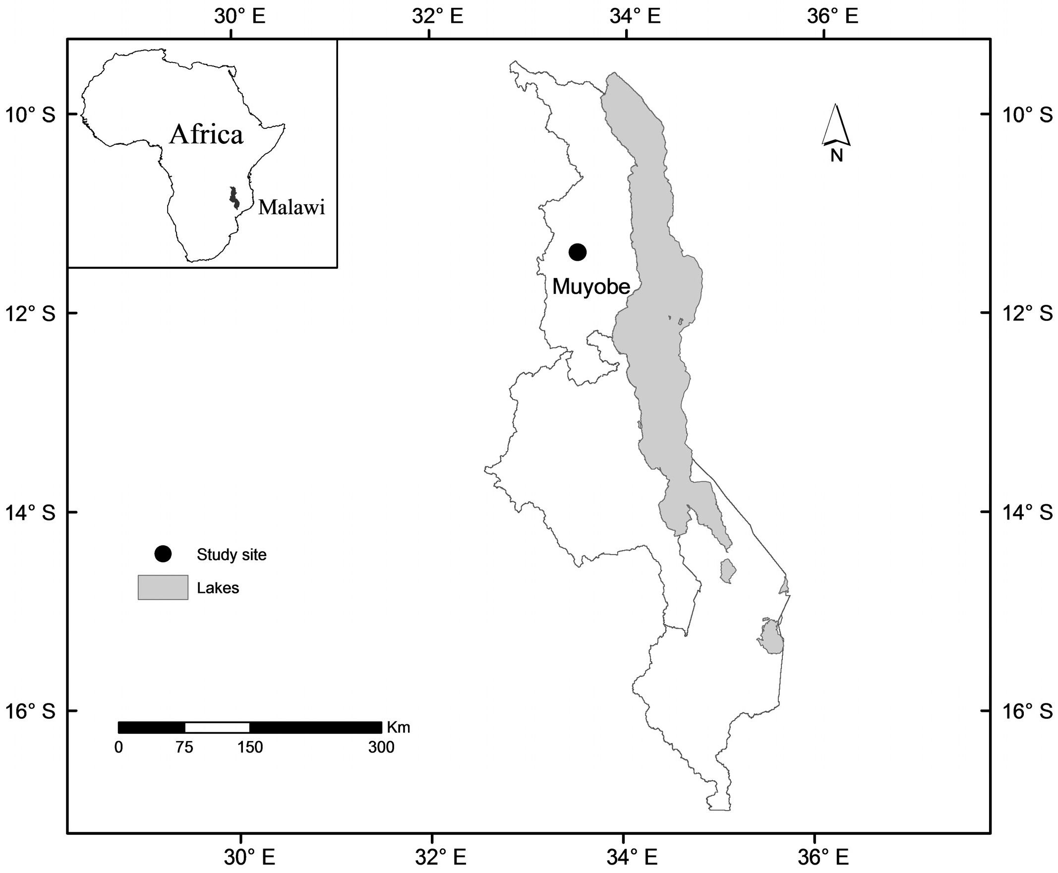
The study area, Muyobe community forest reserve, is located in Mpherembe traditional authority in Mzimba district in the northern region of Malawi (11°35′S, 33°65′E, 1169–1413 m above sea level) (Figure 1). The forest reserve is 486 ha in size, which is common for most small- to medium-sized forests in Malawi. The dominant soil type in the area is Ferrosols [48]. For the nearest weather station in Mzimba, located 69 km south of the study area, the mean annual rainfall was 889 ± 146 mm and the mean annual daily minimum and maximum temperatures were 15 ± 1.6 °C and 26 ± 0.6 °C, respectively, for the period 1975 to 2005. The forest is covered by miombo woodlands dominated by Julbernadia globiflora, Diplorhychus condylocarpon and Combretum zeyheri. For more details on the study area, see Kachamba et al. [32].

2.2. Sampling Design and Field Data Collection

Field reference biomass was based on a systematically distributed probability sample collected from the entire forest reserve. The sample size, i.e., the number of plots, was guided by the budget that could support approximately 100 sample plots. The systematic sample was distributed on a grid of 220 m by 220 m. The grid spacing was calculated as follows:

$$\sqrt{\frac{A}{n}}$$

(1)

where A = size of the forest reserve (m²) and n = is the initial number of sample plots. The grid axes were oriented to the north–south and east–west directions with the starting point randomly selected. Based on the grid, 105 sample plots were located within the boundary of the forest reserve. Field reference biomass was based on data from a forest inventory conducted on the 105 sample plots which were circular (radius = 17.84 m, 0.1 ha each) for 15 days from 25 April to 10 May 2015. Differential Global Navigation Satellite System (dGNSS) was used to ensure precise registration of the positions of centres for field plots. Two Topcon legacy-E + 40 channels dual frequency receivers were used, one operating as a base station and the other as a rover field unit. These receivers observe pseudorange and carrier phase of global positioning system (GPS) and Global Navigation Satellite System (GLONASS). During the study, the baseline between the base station and rover units was approximately 25 km. The position of the base station was determined using Precise Point Positioning (PPP) with GPS and GLONASS data collected continuously for 24 h, as suggested by [49] before the start of the forest inventory. The rover field unit was placed at the centre of each sample plot on a 2.98 m rod for an average of 33 ± 20 min using a one-second logging rate. The recorded sample plot centre coordinates were post-processed using RTKLIB software [50] and the results revealed that the maximum deviations for northing, easting and height were 1.16 cm, 3.02 cm and 3.06 cm, respectively.

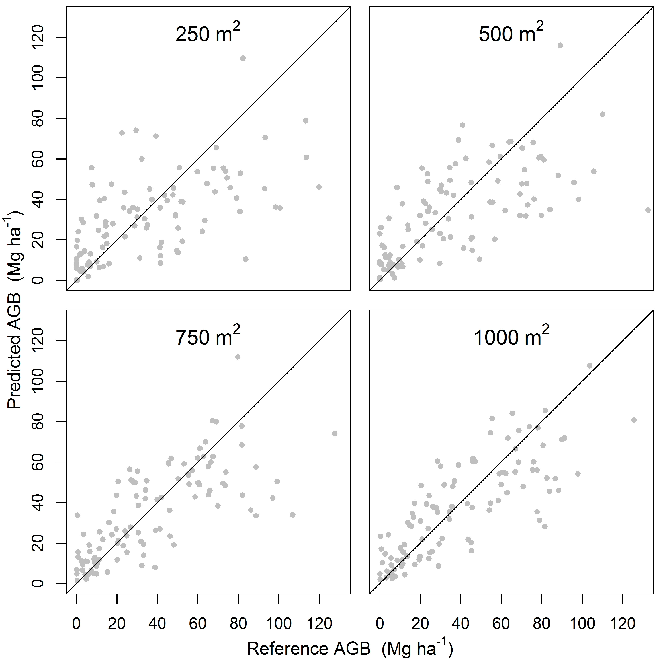
The following information was recorded on each sample plot: diameter at breast height (dbh) (using a caliper or a diameter tape), scientific name and total horizontal distances to sample plot centres of all trees with dbh ≥ 5 cm. The total horizontal distance from a plot centre to each tree was calculated as the sum of the horizontal distance to the front of each tree and half of the tree’s dbh. These distances were subsequently used to subset the sample plot data into different sizes of 250, 500, 750 and 1000 m², respectively, for further analysis. Furthermore, total tree heights (ht) of up to 10 randomly selected sample trees within each plot were also measured. Horizontal distances to sample plot centres and ht measurements were made using a Haglöf vertex hypsometer.

Prior to calculating field reference biomass for each sample plot, we used a height-diameter model developed by Kachamba and Eid [51] to predict the ht of trees whose ht was not measured. Aboveground biomass for the individual trees in each sample plot was then calculated using a model developed by Kachamba et al. [52] with dbh and ht as independent variables. Field reference biomass for the sample plots was subsequently calculated by summing up the individual tree aboveground biomass values within a given distance defined by the radius of the four sample plot sizes. These values were then scaled to per hectare values for the different sample plot sizes. These scaled values were denoted AGB and used as reference values and treated as if they were free from errors, although such plot-wise field values will be subject to both measurement errors and allometric errors.

Table 1. Statistical summary of aboveground biomass (Mg ha⁻¹) for the 105 sample plots based on different sample plot sizes.

Plot Size (m2)	Range	Mean	Std	Cv (%)	Stderr
250	0–150.77	35.63	32.83	92.14	3.20
500	0–132.53	36.83	30.62	83.16	2.99
750	0–127.53	37.65	28.93	76.83	2.82
1000	0–125.59	38.81	29.70	76.53	2.90

Std = Standard deviation, Cv = Coefficient of variation, and Stderr = Standard error.

shows statistical summary of AGB for the different datasets.

2.3. Remote Sensing Data Collection and Processing

2.3.1. UAS Imagery Collection

Image acquisition took place from 23 to 26 April 2015. At this time of the year, the rain season had just ended and the trees still had leaves on them. A SenseFly eBee fixed-wing UAS [53] was used. The UAS was made from flexible foam weighing 537 g without camera. The UAS was equipped with a Canon IXUS127 HS digital RGB (red-green-blue) camera (Canon Inc., Tokyo, Japan). The dimensions and weight of camera with battery and memory card were 93.2 × 57.0 × 20.0 mm and 135 g, respectively. The camera produces 16.1 megapixel images in the red, green and blue spectral bands. The UAS is also equipped with an inertial measurement unit as well as on-board Global Navigation Satellite Systems (GNSS) to control the flight and to provide rough positioning [53].

Prior to taking images, positions of 17 ground control points (GCPs) were identified and measured. The GCPs markers were made of a set of 1 × 1 m cross-shaped timber planks painted white and some black and white 50 × 50 cm checkerboards. The position of the centre of each GCP was fixed using the same procedure used in locating sample plot centres for the sample plot inventory described above. The data were collected for an average of 13 ± 6 min for each GCP with a 1-s logging rate. The recorded coordinates for each GCP were post-processed similarly as the sample plots. The results revealed that maximum deviations for northing, easting and height were 2.24, 4.50 and 4.46 cm, respectively.

Acquisition of images was controlled from a laptop computer with mission control software eMotion 2 version 2.4 (Sensefly, Ltd., Cheseaux-Lausanne, Switzerland) [53]. All the flights were planned in the mission control software prior to flying. For navigation purposes, we used a georeferenced base map from Microsoft Bing maps covering the study area. For this study, we applied percentage end and side image overlaps of 80 and 90%, respectively, as well as a fixed flight height above the ground of 325 m. In total, 22 flights were carried out to cover the forest. A summary of flight characteristics for each flight day is presented in

Table 2. Summary of flight characteristics for each flight block of imagery collection.

Date	Number of Flights	Number of Images	Flight Time (min)	Wind Speed (m s−1)	Cloud Cover (%)
23 April 2015	8	1241	153	6.0–9.5	10–80
24 April 2015	7	1301	146	6.0–9.0	20–80
25 April 2015	6	1118	132	5.0–8.5	10–100
26 April 2015	1	273	26	3.0–4.0	50

. The procedure described here was also applied in Kachamba et al. [32].

2.3.2. Image Processing

Agisoft Photoscan Professional version 1.1 (Agisoft LLC., St. Petersburg, Russia) [54] was used to generate a 3D point cloud from the acquired images. This software uses both structure for motion (SfM) and stereo-matching algorithms for image alignment and multi-view stereo reconstruction. Generation of the point cloud involved the process displayed in

Table 3. Processing steps with corresponding parameter settings in Agisoft Photoscan Professional software for generation of 3D point clouds from unmanned aircraft system (UAS) imagery.

Task	Parameters
(a) Image alignment	Accuracy: high
	Pair selection: reference
	Key points: 40,000
	Tie points: 1000
(b) Mesh building	Surface type: height field
	Source data: dense cloud
	Face count: high
(c) Guided marker positioning	Manual positioning of markers on the 14 GCPs for all the photos where a GCP was visible
(d) Building dense point cloud	Quality: medium
	Depth filtering: mild

. Finally, we added spectral information from the point cloud, i.e., red, green and blue image bands to the point cloud. According to Wallace et al. [55], spectral information from a UAS point cloud can present additional useful information for estimating other non-structural properties of the canopy.

2.3.3. Point Cloud Normalization

The study by Kachamba, Ørka, Gobakken, Eid and Mwase [32], conducted in the same study area, revealed that a digital terrain model (DTM) developed from unsupervised ground filtering of the photogrammetric point cloud performed well. The ground filtering was conducted using a version of the progressive triangular irregular network (TIN) algorithm [56] implemented in Agisoft Photoscan software [54]. The algorithm divides the point cloud into cells of a certain size. In this study, a cell size of 50 m was applied. In each cell, the lowest point is detected and is triangulated to produce a first approximate terrain model. Next, a new point is added to the ground class, providing that it satisfies two conditions: it lies within a certain distance from the TIN and that the angle between the TIN and the line to connect this new point with a point from a ground class is less than a certain angle. This step is repeated while there still are points to be checked. The ground filtering was based on the angle-distance parameter combinations of 3° and 6 m, respectively, as recommended by Kachamba, Ørka, Gobakken, Eid and Mwase [32]. In this study, we applied this DTM to calculate the height relative to the ground for all points by subtracting respective TIN values from each point.

2.3.4. Variable Extraction

Variables describing canopy height were derived from the normalized point cloud and they included maximum and mean values (Hmax, Hmean), standard deviation (Hsd), coefficients of variation (Hcv), kurtosis (Hkurt), skewness (Hskewness) and percentiles at 10% intervals (H₁₀, H₂₀, …, H₉₀). A height threshold of 0.5 m was applied in order to separate tree points from low vegetation and ground. Apart from the variables describing canopy height, variables describing canopy density were derived by dividing the height between a 95th percentile of height and the 0.5 m threshold into 10 equally tall vertical layers and calculating the proportion of points above each layer to the total number of points. These variables were denoted as follows: D₀, D₁, …, D₉. In addition, spectral variables derived from the RGB spectral bands were included. The spectral variables were computed as the maximum (Smax), mean (Smean), standard deviation (Ssd), coefficient of variation (Scv), kurtosis (Skurt), skewness (Sskewness) and nine percentiles (S10, S20, …, S90) for each of the three bands. For example, the Smax variable was denoted as follows: Smax.red, Smax.green and Smax.blue. The remaining spectral variables were also denoted similarly. In total, 64 variables describing canopy height, canopy density and canopy spectral properties were extracted. Some of the extracted height and density variables had missing values for some sample plots for one or several of the plot sizes. In such cases we replaced the missing values with zero in the datasets.

2.4. Model Development and Evaluation

Kachamba, Ørka, Gobakken, Eid and Mwase [32] found that square root-transformed dependent variables performed better than untransformed and logarithmically transformed variables when modelling AGB with variables derived from the UAS imagery. We therefore fit multiple linear regression models relating square root-transformed AGB (as dependent variable) and the calculated variables (as independent variables) for each of the sample plot sizes. Since multicollinearity normally occurs between remotely sensed variables [57], we applied the best subset variable selection procedure using the leaps package [58] in R statistical software [59]. The selection of potential independent variables was restricted to a combination of up to four variables (i.e., based on preliminary tests) with minimum Bayesian information criterion (BIC) and variance inflation factor (VIF) values as selection criteria. An empirical ratio estimator for bias correction proposed by Snowdon [60] was employed when converting predictions to arithmetic scale since square root transformation introduce a bias during back-transformation. The empirical ratio estimator was estimated from the ratio of the mean of the observed values to the mean of the back-transformed predicted values. The estimates were finally corrected by multiplying them with the estimated ratio.

For each model, reported values included root mean square error (RMSE), relative root mean square error (RMSE%), mean prediction error (MPE), relative mean prediction error (MPE%) and squared Pearson’s correlation coefficient (r²). However, comparison of the models was based on RMSE values. RMSE is a reliable measure for model performance as it accounts for both variance and bias of the predicted value [61]. RMSE, MPE, RMSE% and MPE% were calculated as follows:

$$\mathrm{RMSE}=\sqrt{\frac{{\sum }_{i=1}^{\mathrm{n}}(y_i-{\widehat{y}}_i{)}^2}{n}}$$

(2)

$$\mathrm{MPE}=\frac{{\sum }_{i=1}^n\left(y_i-{\widehat{y}}_i\right)}{n}$$

(3)

$$\mathrm{RMSE}\text{\%}=\frac{\mathrm{RMSE}}{\overline{y}}\times 100$$

(4)

$$\mathrm{MPE}\text{\%}=\frac{\mathrm{MPE}}{\overline{y}}\times 100$$

(5)

where $y_i$ is the AGB field value for plot i and ${\widehat{y}}_i$ is the predicted AGB for sample plot i, respectively, n is the number of plots and $\overline{y}$ is mean AGB for all plots.

Both RMSE and MPE values were calculated using leave-one-out cross validation. The MPE value of each model was tested to check for statistical significance using two-sided student’s t-tests with α = 0.05.

2.5. Biomass Estimation Methods

2.5.1. Field-Based Sample Estimation

We applied a simple random sampling estimator to estimate AGB and standard errors of AGB estimates based on the sample plots [61]. Application of systematic sampling design brings positive bias on the estimates [62]. However, according to Gregoire and Valentine [61], this bias is negligible and unknown as it is a property of the estimator and not a particular sample [61]. Since the focus of the analysis in the current study was on the assessment of the influence of sample plot sizes on the precision of the estimates, we assumed that the calculated variance estimates based on the simple random sampling design were adequate for the task at hand. We thus estimated mean AGB per hectare for the study area as follows:

$${\widehat{B}}_{\mathrm{field}}=\frac{{\sum }_{i=1}^n{y}_i}{n}$$

(6)

where $y_i$ is AGB for plot i and n is the total number of sample plots.

The variance for the estimator in (6) was estimated as follows:

$$\widehat{V}({\widehat{B}}_{\mathrm{field}})\frac{{\sum }_{i=1}^n{\left(y_i-{\widehat{B}}_{\mathrm{field}}\right)}^2}{n\left(n-1\right)}$$

(7)

where $\widehat{V}{(\widehat{B})}_{\mathrm{field}}$ is the variance estimator for estimated mean AGB.

2.5.2. UAS-Assisted Estimation

First, the study area was tessellated into grid cells using regular grids with sizes equivalent to respective sample plot sizes, i.e., 250 m², 500 m², 750 m² and 1000 m² for the purpose of estimating AGB for the entire area. For each grid cell, variables were derived from the image data as described from the sample plots above. For each of the plot size, the previously fitted regression model (Section 2.6) was applied to predict AGB values for each grid cell. Then mean AGB for the study area was estimated based on the model-assisted regression estimator described in Särndal et al. [63] (Page 231) as follows:

$${\widehat{B}}_{\mathrm{UAS}}=\frac{{\sum }_{i=1}^N{\widehat{y}}_i}{N}+\frac{{\sum }^{\text{}}\left(e_i\right)}{n}$$

(8)

where $\widehat{y}$_i is predicted AGB for the ith grid cell, N is the total number of grid cells for the study area and $e_i$ = $y_i$ − ${\widehat{y}}_i$ is the model prediction residual for plot i.

The variance for the model-assisted regression estimator was estimated as follows [63] (p. 234):

$$\widehat{V}({\widehat{B}}_{\mathrm{UAS}})=\frac{{\sum }_{i=1}^n{(e_i-\overline{e})}^2}{n(n-1)}$$

(9)

where $e_i$ is the model prediction residual for plot i and $\overline{e}$ = $\frac{{\sum }_{i=1}^n{e}_i}{n}$ is the mean residual for all plots.

2.5.3. Efficiency of UAS-Assisted Estimations

The relative efficiency (RE) of UAS-assisted over the field-based inventories was calculated as follows:

$$\mathrm{RE}=\frac{\widehat{V}({\widehat{B}}_{\mathrm{field}})}{\widehat{V}({\widehat{B}}_{\mathrm{UAS}})}$$

(10)

where RE is the relative efficiency of UAS-assisted over field-based inventories, $\widehat{V}({\widehat{B}}_{\mathrm{field}})$ is the variance of the field-based biomass estimate (Equation (7)) and $\widehat{V}$(${\widehat{B}}_{uav}$) is the variance of the UAS-assisted biomass estimate (Equation (9)).

An RE value greater than 1.0 indicates higher efficiency of UAS-assisted estimates than field-based estimates for a given plot size (see [64]). For each of these datasets, biomass estimates, standard error of the estimate (SE) and RE values were calculated for both field-based and UAS-assisted. The SE values were calculated as the square root of the variance of the biomass estimates based on field-based and UAS-assisted inventories, respectively.

2.6. Cost Efficiency Analysis

During field work, we randomly selected 16 sample plots and for each plot recorded three categories of time consumption, i.e., fixed time (time spent when recording sample plot attributes such as plot number, date, etc.), variable time (time spent on measuring trees) and walking time (time spent during walking from one plot to another). The average recorded time consumption was 7.5, 25.0 and 7.0 min for each of the categories, respectively. We then set the relative cost of a sample plot inventory of 105 sample plots (1000 m² each) in a 220 m by 220 m grid to 100% based on the recorded information. We then used the cost information from the current inventory (4 persons working for 15 days with a daily salary of USD 25.13 each) to calculate the variable costs for each plot scaled according to plot size and walking distance.

The costs of UAS data acquisition were fixed for all sample plot sizes because the need for auxiliary remotely sensed information would be the same regardless of plot size. The cost was computed based on the experience from the current study. The costs included pre-flight preparations and the actual flying where a two-man crew was required. Each person worked five days with a salary similar to the field crew. Post-processing of the acquired images required four days.

3. Results

3.1. Model Performance Based on Different Sample Plot Sizes

For assessment of the effect of sample plot sizes on model performance, we fit regression models using the data from the different sample plot sizes based on a leave-one-out cross validation procedure. None of the models had MPE values that were significantly different from zero (p > 0.05) (

Table 4. Model performance over different sample plot sizes *.

Plot Size (m2)	r2	Independent Variables a	Predicted AGB Mg ha−1	RMSE		MPE
				Mg ha−1	%	Mg ha−1	%	p-Value
250	0.31	Hmax, H20.red	35.82	28.68	80.50	−0.19	−0.52	0.96
500	0.44	Hmax, H10.red	37.40	24.23	65.79	−0.58	−1.56	0.81
750	0.54	Hcv, D1, Hsd.blue	37.81	21.07	55.96	−0.15	−0.40	0.94
1000	0.64	Hmax, H70.red, H90.green	39.33	20.13	51.86	−0.52	−1.34	0.79

* Predicted AGB, RMSE and MPE based on leave-one-out cross validation. ^a See text for variable description.

). The models produced RMSE% values (on arithmetic scale) in the range of 51.86–80.50% of the mean AGB from the respective sample plot sizes. The model for sample plot size 1000 m² produced the smallest RMSE% value amongst the models. On the other hand, the model based on a sample plot size of 250 m² produced the highest RMSE% value. The RMSE% values decreased as the sample plot sizes increased. However, the pattern for MPE% values with increase in sample plot size is irregular (see Table 4). The r² values for the final models ranged from 0.31 to 0.64. The model for sample plot size 1000 m² produced the highest r² value amongst the developed models. On the other hand, the model based on a sample plot size of 250 m² produced the smallest r² value (see Table 4). Figure 2 displays the relationship between field reference and predicted AGB for the different plot sizes. The results indicate a pattern of under prediction of AGB for higher AGB values for all plot sizes.

The models contained a minimum of two and a maximum of three independent variables. All the models contained variables describing canopy height. Further, the models contained variables incorporating red, green and blue spectral bands. One of the models incorporated a variable describing canopy density.

3.2. Assessment of the Efficiency of UAS-Assisted AGB Estimation

The standard error (SE) values for field-based AGB estimates were larger compared to those of UAS-assisted for all sample plot sizes (

Table 5. Estimated mean AGB and associated standard error (SE) estimates based on field-based and UAS-assisted estimation for different sample plot sizes.

Plot Size	Field-Based (Mg ha−1)		UAS-Assisted (Mg ha−1)		RE
(m2)	$\widehat{\mathit{B}}$field	SE	$\widehat{\mathit{B}}$UAS	SE
250	35.63	3.20	37.56	2.68	1.43
500	36.83	2.99	38.49	2.26	1.75
750	37.65	2.82	38.88	1.91	2.18
1000	38.81	2.90	40.97	1.75	2.75

$\widehat{B}$_field = Estimated mean AGB from field-based sample, $\widehat{B}$_UAS = Estimated mean AGB from UAS-assisted estimation, SE = Estimated standard error of mean AGB.

). The RE values showed an increasing trend with increasing sample plot sizes (Table 5).

3.3. Cost Efficiency Analysis

The smallest SE was obtained using 1000 m² sample plot size in a UAS-assisted inventory. However, relative cost of this inventory was the highest amongst the tested sample plot sizes (Figure 3). Furthermore, the decrease in standard error was larger for UAS-assisted compared to field based when increasing plot size. Thus, there is a trade-off between inventory costs and required precision. Our results show that small sample plots are desired to keep the inventory cost low. However, if a standard error of less than approximately 3 Mg ha⁻¹ was targeted, then a UAS-assisted forest inventory should be applied to ensure more cost effective and precise estimates.

4. Discussion

Integration of efficient forest inventory techniques in biomass estimation is key to the successful implementation of the REDD+ mechanism. This study aimed at estimating the efficiency of a UAS-assisted inventory for estimation of biomass based on different sample plot sizes in a forest reserve in miombo woodlands of Malawi which is typical for the size and properties of such reserves in the country. Thus, the results may be of general interest and relevance beyond the scope of this case study. The study has demonstrated that incorporating UAS-derived photogrammetric data in a forest inventory can improve biomass estimates beyond what can be achieved by purely field-based sample inventories. The relatively small SE values for the UAS-based estimates indicate that inclusion of remotely sensed data from UAS imagery can improve the precision of the biomass estimates. Thus, the application of UAS-assisted inventories for REDD+ implementation in Malawi could potentially result in improved biomass estimates compared to pure field-based inventories.

Just like in any remote sensing assisted forest inventory, the precision of biomass estimates based on a UAS-assisted inventory is highly influenced by the choice of sample plot sizes [38]. This is demonstrated by several aspects in the results. First, the trends in the RE values show that the magnitude of the efficiency of UAS-assisted inventories is influenced by the sample plot size employed. For instance, the average RE values for the 250, 500, 750 and 1000 m² sample plot sizes were 1.43, 1.75, 2.18 and 2.75, respectively, indicating an increase in the magnitude of the efficiency of UAS-assisted inventory with increasing sample plot sizes.

As in our study, systematic designs are often applied in forest inventories because they are more efficient. However, when the sampling intensity is small for any sampling design, the risk of not capturing the whole range of the variable of interest increases. Subsequently, poorer predictive models are developed thus leading to extrapolation when predicting forest attributes in forests with attributes that are not represented in the field data. In order to develop a good predictive model, more efficient sampling designs should be adopted by spreading the sample in the space of the variables derived from the remotely sensed data [65,66]. This issue should therefore be taken into account when planning future UAS forest inventories.

The influence of sample plot sizes was further demonstrated by the trends in RMSE values. The results have shown that the RMSE values decreased by approximately 30% between the smallest (250 m²) to the largest (1000 m²) sample plot sizes. The same trend was observed by Frazer, Magnussen, Wulder and Niemann [38] and Mauya, Hansen, Gobakken, Bollandsås, Malimbwi and Næsset [15] (see

Table 6. Effect of sample plot sizes on the root mean square errors (RMSE) of biomass estimates for different studies.

Studies	Sample Plot Size (m2)	RMSE (Mg ha−1)	Change (%)	Remotely Sensed Data
Frazer, Magnussen, Wulder and Niemann [38]	314–1964	157.60–97.80	37.94	ALS
Mauya, Hansen, Gobakken, Bollandsås, Malimbwi and Næsset [15]	200–3000	262.47–93.73	64.29	ALS
Current study	250–1000	28.68–20.13	29.81	UAS

). The magnitude of the decrease in RMSE values reported are quite varied due to differences in the range of sample plot sizes.

The improvement of biomass estimates with increasing sample plot sizes shows that large sample plot sizes favour UAS-assisted inventories. This could be attributed to reduction in plot boundary effects as the sample plot sizes increases, as suggested by Goetz and Dubayah [67]. Thus, for small sample plots, canopies of trees with wide crowns such as those in miombo woodlands [68] tend to be partially included and thus under-predicting sample plot biomass. On the other hand, as the sample plot sizes increase, this effect tends to decrease substantially since these variations are averaged out at larger sample plot sizes [43].

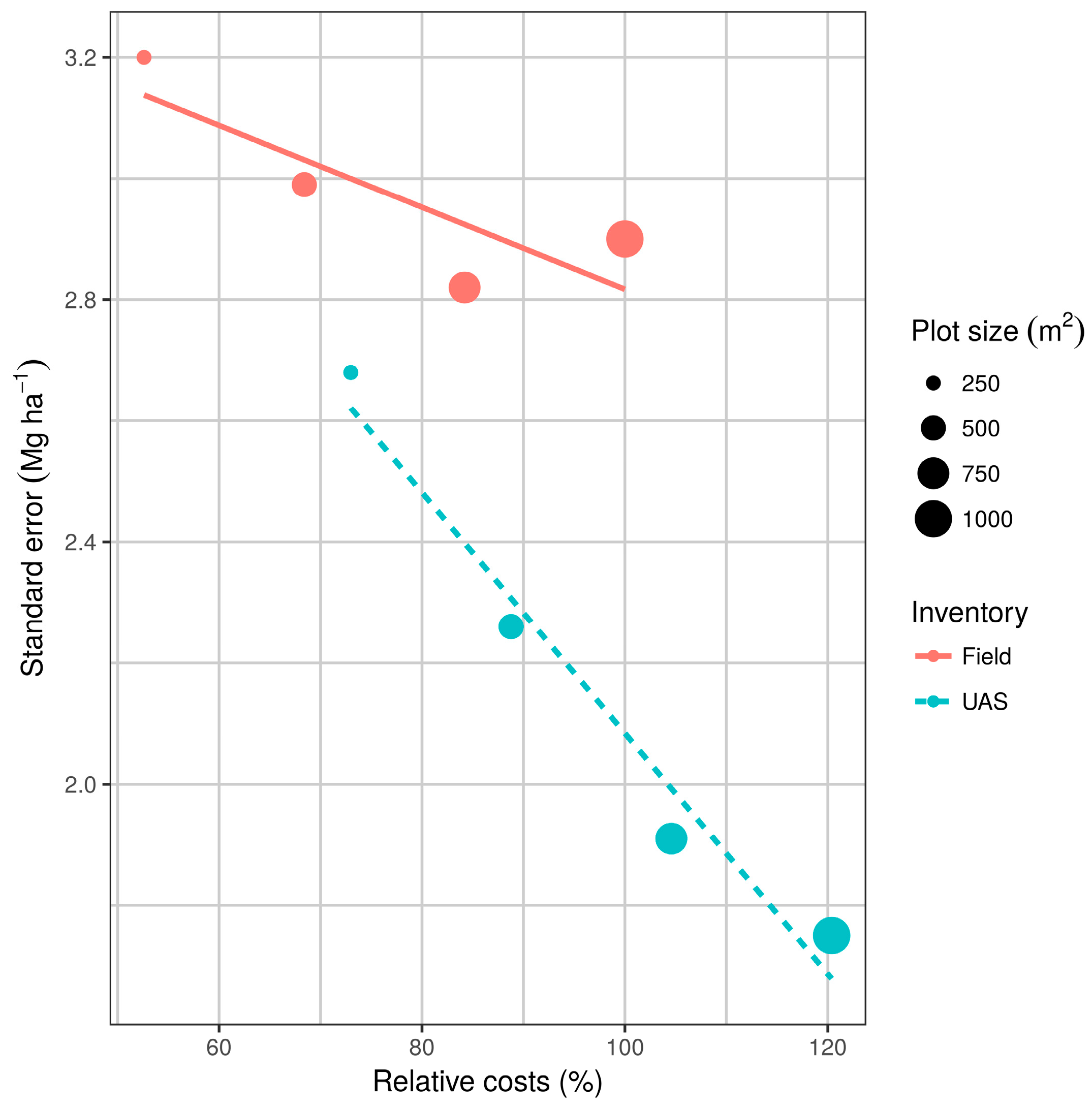
The fact that the results in the current study indicate that larger plots favor UAS-assisted forest inventories does not imply that larger plot sizes should always be applied during the UAS-assisted inventory because of the associated costs. The results of the cost efficiency analysis presented in Figure 3 indicate that there is a trade-off between costs and required precision. On one hand, acquiring UAS data and field reference data from many large plots is expensive but produces more precise results. This demonstrates the need for carrying out a cost analysis during UAS-assisted inventory in order to determine the optimal sample plot size.

Finally, it should be noted that careful planning is needed for application of UAS-assisted inventories under the REDD+ mechanism in Malawi to be accomplished. For example, if the inventory is intended for smaller forest reserves, wall-to-wall coverage using a UAS is possible. On the other hand, in cases where inventories are conducted in larger forest reserves, the UAS can be applied as a sampling tool because wall-to-wall operations may be found economically and logistically infeasible. Furthermore, this study was conducted on a single site and thus represents a forest inventory scenario at a specific location. Although this case study has provided evidence of great efficiency of UAS-assisted inventory, similar studies should be conducted in other reserves across the country in order to be able to generalize and provide guidance for future operational inventories.

5. Conclusions

Successful incorporation of UAS-based remote sensing technologies for biomass estimation in REDD+ projects in Malawi requires studying the influence of key factors, such as sample plot size, which affect the precision of the estimates. The study has demonstrated that UAS-assisted inventories tend to produce more precise estimates compared to those utilising exclusively field-based methods. Furthermore, larger sample plot sizes tend to favor UAS-assisted inventories. We therefore recommend that UAS-assisted inventories be incorporated in the implementation of REDD+ in Malawi to improve biomass estimates. However, more studies are needed to check the influence of sample plot sizes for different study sites where costs are also considered.