
Region-of-Interest Extraction Based on Local–Global Contrast Analysis and Intra-Spectrum Information Distribution Estimation for Remote Sensing Images


1
The College of Information Science and Technology, Beijing Normal University, Beijing 100875, China
2
The State Key Laboratory of Remote Sensing Science, Beijing Normal University, Beijing 100875, China
*
Author to whom correspondence should be addressed.
Remote Sens. 2017, 9(6), 597; https://doi.org/10.3390/rs9060597
Submission received: 27 March 2017
/
Revised: 25 May 2017
/
Accepted: 7 June 2017
/
Published: 12 June 2017
Abstract
:Traditional saliency analysis models have made great advances in region of interest (ROI) extraction in natural scene images and videos. However, due to different imaging mechanisms and image features, those approaches are not quite appropriate for remote sensing images. Thus, we propose a novel saliency analysis and ROI extraction method for remote sensing images, which is composed of local–global contrast analysis for panchromatic images and intra-spectrum information distribution estimation (LI) for multi-spectral images. The panchromatic image is first segmented into superpixels via level set methods to reduce the subsequent computation complexity and keep region boundaries. Then, the spatially weighted superpixel intensity contrast is calculated globally to highlight superpixels unique to others and obtain the intensity saliency map. In multi-spectral images, ROIs are often included in informative superpixels; therefore, the information theory is introduced to each spectrum independently to acquire the spectrum saliency map. The final result is obtained by fusing the intensity saliency map and the spectrum saliency map and enhancing pixel-level saliency. To improve the anti-noise properties, we employ the Gaussian Pyramid for multi-scale analysis, which removes noise points by the blurring operation and the down-sampling operation. Experiments were conducted aiming at comparing the LI model with nine competing models qualitatively and quantitatively. The results show that the LI model performs better in maintaining intact ROIs with well-defined boundaries and less outside interference, and it tends to be stable when faced with images contaminated by noise.
1. Introduction
A region of interest (ROI) is a selected subset of samples within a data set identified for a particular purpose [1]. In geographical information systems, a ROI can be taken literally as a polygonal selection from a 2D map. ROI extraction is one of the most important fields in remote sensing image analysis since it can be applied to image compression, image fusion, target extraction and change detection [2,3,4]. Traditional top-down ROI extraction approaches usually include classification and depend on prior knowledge libraries, which are inconvenient to build. They are very time-consuming because global searching is an indispensable part in the processing. Moreover, with the rapid development of remote sensing technology, the resolution of remote sensing images increases, and the intensity, structure, shape and texture information are more abundant [5,6,7,8]. Due to the irregular shape, unfixed size and other characteristics of ROIs, the extraction accuracy cannot be guaranteed when traditional methods are applied to high-resolution remote sensing images. Thus, accurate and fast ROI extraction for high-resolution images has become a significant issue in remote sensing and information interdisciplinary research [9,10].
Studies on the human visual system (HVS) offer a valuable perspective. The mechanism of the HVS serves as a filter to select only the interesting information related to current behaviors or tasks to be processed while ignoring irrelevant information [11,12]. Koch and Ulman [13] first introduced the concept of the saliency map and combined visual features with a winner-take-all neural network. Their model has become the basis of subsequent models, including Itti’s model. Itti et al. [14] completed the implementation and verification of Koch and Ullman’s model first and then applied it to natural and synthetic images (ITTI). Goferman et al. [15] proposed a context-aware (CA) saliency detection model that analyzed saliency locally and globally at different scales, emphasizing the context. Meur et al. [16] suggested a coherent computational approach to the modeling of the bottom-up visual attention. Ma et al. [17] computed the local spatial contrast of image intensity at each location. They argued that locations with high feature contrast had rich information most of the time. However, biological models that try to process images on the basis of the HVS biological construction often lead to unavoidable computational complexity and neglect the characteristics in the frequency domain [18].
Researchers also proposed some purely computational models [19,20]. Hou et al. [21] extracted the spectral residual (SR) from the input image in the spectral domain based on the Fourier Transform and proposed a fast way to form a corresponding saliency map in the spatial domain by analyzing the log-spectrum. Nevertheless, the saliency map is low-resolution and unavoidably abandons many details, which limits the application of the method to small-format images. Imamoglu et al. [22] presented a novel bottom-up model based on visual attention to acquire the saliency maps using wavelet transform (WT). Various feature maps were obtained by the inverse Wavelet transform with the band-pass regions of the image at different scales. Using those features, the local and global saliency maps were generated to form the final saliency map. Rosin [23] suggested an edge-based ROI detection method assuming that dense regions in an edge map were likely to be interesting locations. The model only focuses on the edges of objects, which is prone to introducing inner holes to the extraction results and losing much detail information of the targets.
Some researchers have tried to combine biological and computational models. Harel et al. [24] proposed the Graph-Based Visual Saliency (GBVS) model. They introduced ideas from graph theory to concentrate mass on activation maps and formed activation maps from raw features. The saliency map yielded by the model is also low-resolution and discards some spatial information. Achanta et al. [25] proposed a frequency-tuned (FT) method for computing saliency using low level features, such as color and luminance, which was easy and fast to implement and could provide full-resolution saliency maps. However, it works well only on images that have large and homogeneous objects with clear boundaries.
Recently, some region-based methods have drawn much attention. Shi et al. [26] introduced a hierarchical (H) saliency detection model. They first produced an over-segmentation image and redefined the “scale” for a region as the side length of the largest square it could hold. Then, regions under a particular scale threshold were merged to their nearest neighbors in terms of average color distance. Saliency maps of various scales were obtained by varying the threshold and were fused into one saliency map by a tree-structure graphical model. Cheng et al. [27] presented a region contrast based model for salient region detection. After segmenting the image into regions, they computed the saliency value for a region by measuring its color contrast and spatial position to all the other regions. Nevertheless, those region-based models often neglect the integrity with holes inside ROIs, leading to incomplete extraction results. They also detect some fragments in the background.
Some researchers directly segment the input image into square or rectangular regions with fixed size, which neglects the local correlation. The concept of superpixel was first introduced by Ren [28] to segment input images into coherent and correlative regions for the purpose of simplifying computations. Superpixels represent a restricted form of region segmentation, balancing the conflicting goals of reducing image complexity through pixel grouping while avoiding under-segmentation [29]. Aggregating neighboring pixels into superpixels can not only reduce the complexity of subsequent processing but also maintain the boundary information.
Traditional saliency analysis models are efficient in extracting ROIs such as flowers, animals and human beings in natural scene images and videos [30,31,32,33]. However, if they are directly applied to ROI extraction in remote sensing images, the results may be undesirable because of different imaging mechanisms and image features. Recently, some researchers have proposed saliency analysis algorithms especially for ROI detection in remote sensing images [34,35]. Wang et al. [36] employed edge detection, preliminary line extraction and an improved Hough transform to detect ROIs in remote-sensing images. Zhang et al. conducted in-depth researches and proposed a multiscale feature fusion (MFF) model [37] and a frequency domain analysis (FDA) model [38]. In the MFF model, the multiscale spectrum residuals method was used to compute intensity saliency, and the interpolating biorthogonal integer wavelet transform was used to extract orientation features. Finally, they introduced a weighted across-scale fusion strategy to fuse saliency maps of various scales into one saliency map. In the FDA model, the input remote sensing image was converted into HSI space, and the quaternion Fourier transform was employed to generate the saliency map.
Given the characteristics of high-resolution remote sensing images, we list the requirements that high-quality ROIs should meet:
- (1)
- Well-defined boundaries: Accurate ROIs are conducive to image compression, image registration and change detection. This problem can be solved by superpixel segmentation since superpixels usually maintain much boundary information.
- (2)
- Complete ROIs without inner holes: In remote sensing images, because of the complex texture information in ROIs, there is a high likelihood of obtaining ROIs with inner holes. However, applications such as image compression and image registration need all of the information for ROIs.
- (3)
- No interference outside of the ROIs: Some interference is often detected when we extract ROIs. For example, when ROIs are residential areas from high-resolution remote sensing images, shades of mountains and discontinuous roads are easily detected interference.
To meet the requirements above, we propose a saliency detection model for ROI extraction in remote sensing images, which is composed of local–global contrast analysis for panchromatic images and intra-spectrum information distribution estimation (LI) for multi-spectral images. The major contributions of our paper are: (1) for the panchromatic image, superpixels with similar size and well-defined boundaries are obtained by segmentation and then treated as basic processing units to compute the intensity saliency map; (2) for multi-spectral images, we exploit their information complementarity to the panchromatic image and introduce the information theory to calculate the spectrum saliency map; and (3) a pixel-level saliency enhancement strategy is presented to highlight the salient objects and suppress the non-salient objects.
2. Methodology
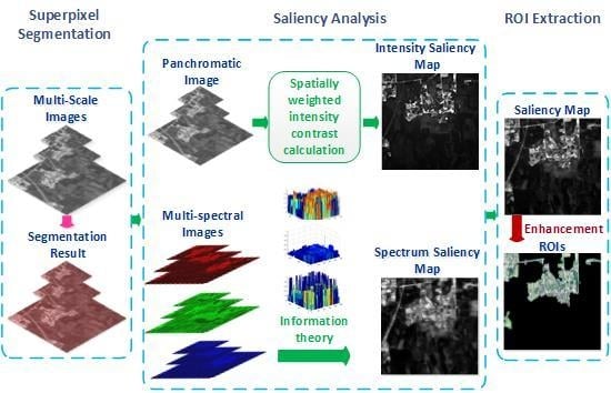
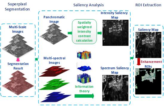
In this section, we explain the LI model in detail. First, the input panchromatic image is segmented into superpixels to reduce the subsequent computation complexity and keep region boundaries. Figure 1a shows the segmentation steps; we will explain the steps in detail later in Section 2.1. For the panchromatic image, the intensity saliency map is acquired by calculating the spatially weighted intensity contrast between superpixels globally. For multi-spectral images, the theory of information is introduced to each spectrum independently to compute multi-spectral information maps. The spectrum saliency map is generated by fusing various information maps and then calculating the information of superpixels. To alleviate the influence of noise, we apply above steps to multi-scale images obtained by the Gaussian Pyramid and generate multi-scale intensity saliency maps and multi-scale spectrum saliency maps. Then, the across-scale fusion is performed to produce the intensity saliency map and the spectrum saliency map. The process is shown in Figure 1b. The final saliency map, which is obtained by combining the intensity saliency map and the spectrum saliency map and enhancing pixel saliency, is segmented into a binary mask using the threshold provided by the Otsu method [39]. ROIs are acquired by the logical AND operation of the binary mask and the colored image synthesized by multi-spectral images; Figure 1c shows the steps.
2.1. Superpixel Segmentation
With the increasing resolution of remote sensing images, pixel-based analysis will cause high complexity. If pixels with similar features can be aggregated into one group by image segmentation and the subsequent analysis is performed on groups, the computation complexity will be reduced greatly. Traditional methods for segmentation such as local variation, mean-shift and watershed can lead to under-segmentation in the absence of boundary cues in the image. Some researchers have proposed specific superpixel segmentation methods for remote sensing images [40,41]. However, their purposes are primarily to segment the whole image into specific regions, and the results are not suitable for our subsequent analysis.
In this paper, we introduce a superpixel segmentation method [29] that focuses on uniform size, coverage, connectivity, compactness, edge-preservation and no overlap to remote sensing images. Level-set methods are used to generate superpixel boundaries. The steps are shown roughly in Figure 1a. Given the number of superpixels , seeds are put into a lattice formation so that distances between lattice neighbors are all approximately equal to , where is the number of pixels in the image. Especially, seeds should be put away from high gradient regions. The above operation guarantees similar size for superpixels. Then, seeds are set to “assigned” and the other pixels to “unsigned”. Boundaries are evolved by the following function, and the skeleton of the unassigned region is estimated:
In practice, is defined over the image plane as the signed Euclidean distance of each pixel to the closest point on the boundary between the assigned and unassigned (background) regions. A pixel’s distance is positive if it is in the unassigned region and negative if it is not, with the boundary represented implicitly as the zero level set of . represents one “time stage” in the evolution process.
depends on the local image structure and superpixel geometry at each boundary point, and depends on the boundary point’s proximity to other superpixels. is a local affinity function based on grayscale intensity gradient and it produces high velocities in areas with low gradients, with an upper bound of 1. is the curvature of the zero level set at point , and and are balancing factors. works as a binary stopping term to ensure that the boundaries of nearby superpixels never cross each other. For example, if and only if is on the 2D homotopic skeleton of the unassigned region, and everywhere else. is the normal of .
Speeds of pixels on the boundary and of unassigned pixels in the boundary’s immediate vicinity should also be updated until speeds of pixels on the boundaries are around 0. The evolution stops when the relative increase of the total area covered by superpixels is less than . Then, the evolution results are post-processed to obtain one-pixel-width boundaries. The post process includes three steps: (1) any remaining large unassigned connected regions are regarded as superpixels; (2) very small superpixels are removed and pixels in them are treated as unassigned; and (3) unassigned regions are thinned by the algorithm in [42]. The segmentation steps and the results are shown in detail in Figure 2. We use this method to segment the panchromatic image into superpixels.
2.2. Saliency Analysis
Satellite sensors usually provide two types of data: the panchromatic image and multi-spectral images. Thus, saliency analysis is performed focusing on those two kinds of data, including the local–global contrast analysis for panchromatic images and the intra-spectrum information distribution estimation for multi-spectral images.
2.2.1. Local–Global Contrast Analysis
Intensity is one of the conspicuous characteristics of the image for saliency analysis [43], which is used by Itti in [13] to generate feature maps via Gaussian pyramid. The panchromatic image lacks color and spectrum information; thus, the difference in intensity is quite significant in distinguishing ROIs from backgrounds. In this paper, we compute the spatially weighted intensity contrast for superpixels to obtain the intensity saliency map.
A superpixel is more likely to be salient if it is unique to other superpixels. In some studies, the superpixel saliency is decided by its contrast to neighboring superpixels, and authors often provide their own definitions of “neighboring”, which regard saliency as a local concept and may cause disaccord in implementation. In Section 2.1, the superpixel segmentation method has already taken local intensity information, such as connectivity and compactness, into consideration. Therefore, saliency should be considered globally by comparing one superpixel with all the other superpixels. We follow this idea and obtain the saliency value for a superpixel by calculating its intensity contrast to all the other superpixels. For superpixel , the following formulas are used to calculate its intensity contrast to superpixel :
where is the intensity of the th pixel in and is the number of pixels in .
However, those contrasts have different influences because of different spatial positions. The farther two superpixels are apart, the less influence their contrast has. Thus, the superpixel contrast should have a corresponding spatial weight. Accordingly, the weight of Cij is defined as follows, which is determined by the Euclidean distance between and :
where is the centroid of and represents the 2-norm. is a factor that controls the effect of distance.
The saliency value of is determined by its weighted intensity contrast to all the other superpixels, as can be computed as follows:
The saliency value of a pixel is the saliency value of the superpixel it belongs to. Then, we acquire the intensity saliency map .
2.2.2. Intra-Spectrum Information Distribution Estimation
The image saliency is related to the distribution of pixels. A general contrast principle states that rare or infrequent visual features in a global image context give rise to high saliency values [44]. Theoretically, the aim of saliency analysis is to find regions that are most informative in images, and ROIs are always more informative than non-ROIs. Shannon defines the amount of information a message contains as the negative value of its logarithm probability:
where represents the probability of occurrence for the grayscale of pixel . From the formula above, we can learn that the less the probability is, the more information the message has, which is consistent with the general contrast principle. Thus, for every pixel in every spectrum, we use Formula (10) to compute its amount of information and obtain multi-spectral information maps. Images used for experiments have 256 grayscales and traditional methods usually construct a histogram to calculate the probability. After many experiments, we find that the results exhibit little difference when the number of grayscales is more than eight. When the number is less than eight, the results begin to show great difference with the number decreasing. Therefore, we reduce the number of grayscales to eight to be efficient with reasonable results. Those information maps are fused into one information saliency map according to the following formula:
where indexes different spectra and is the information map for spectrum .
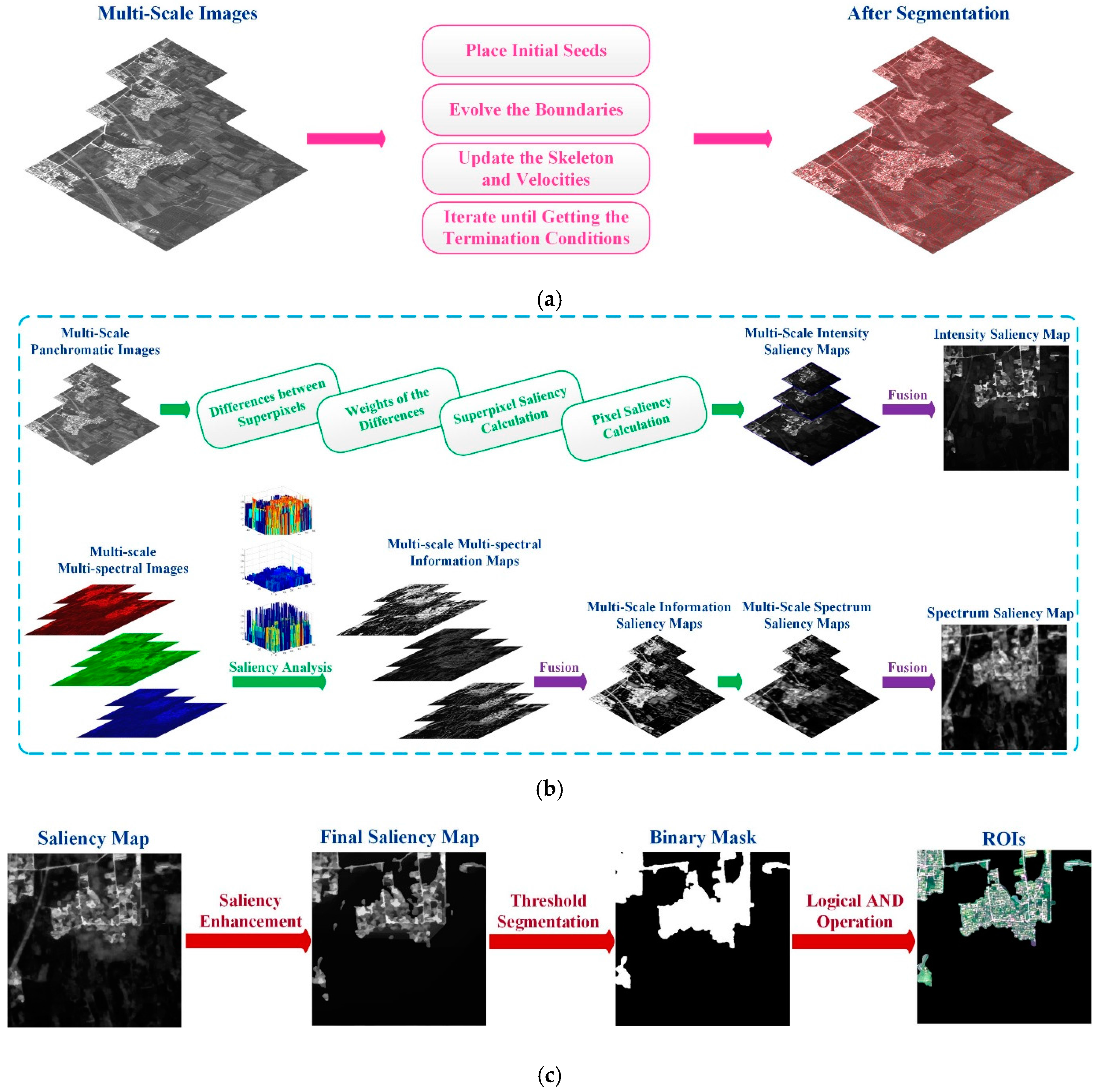
However, as can be seen in Figure 3, some interference in the backgrounds appears infrequently and thus is given higher saliency values in the information saliency map, which will act as noise in the extraction results and is undesirable. Since superpixels have been generated in Section 2.1, we are enlightened by Reference [45] and use the superpixel segmentation result to calculate the superpixel information for the information saliency map, which can remove single noise points to some extent. We define the amount of information for as summing the amount of information of pixels belonging to :
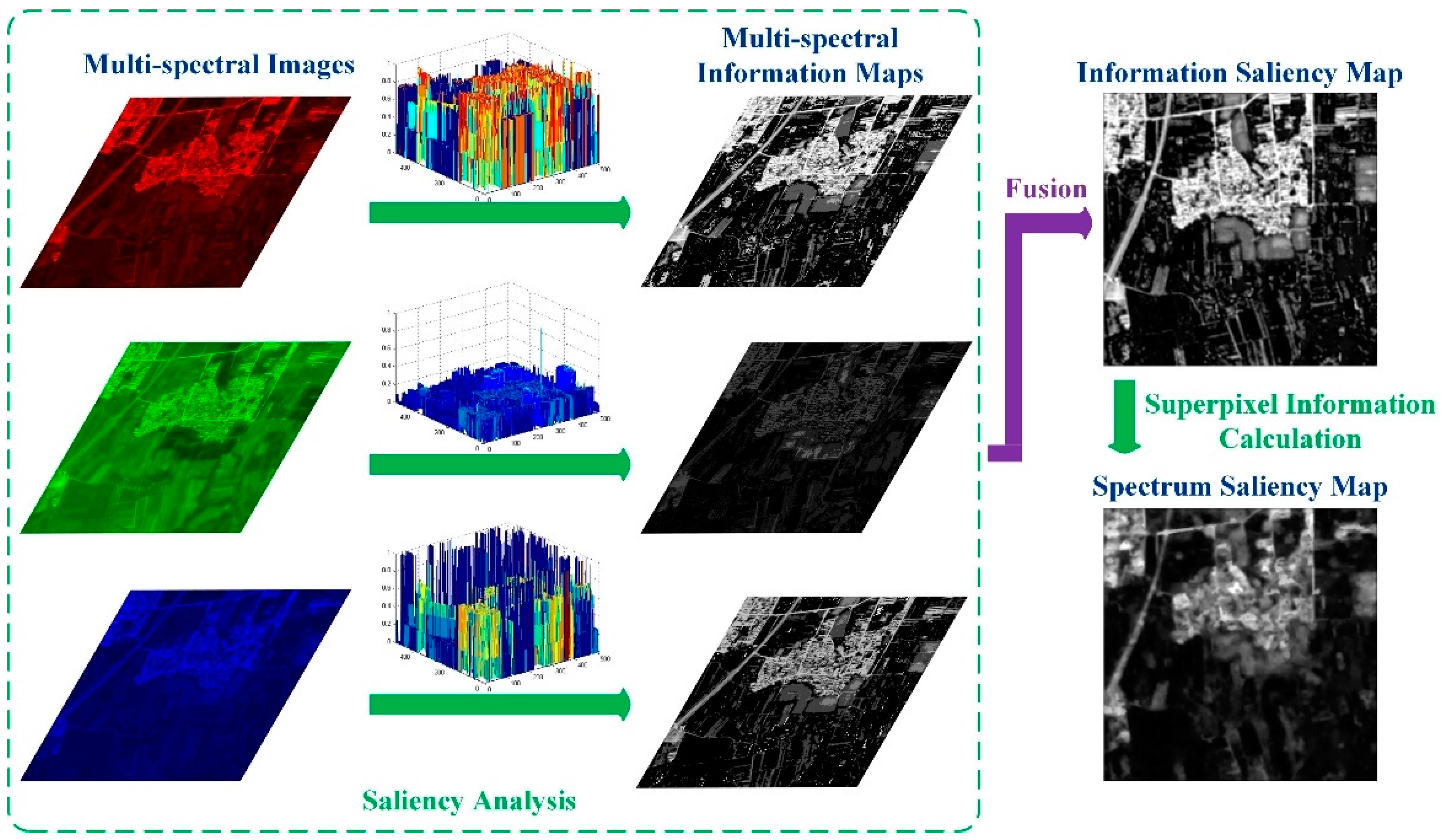
where corresponds to the value of the th pixel in in the information saliency map and is the number of pixels in . As has been previously stated, the saliency value of a pixel is equal to the saliency value of the superpixel it belongs to. After processing all the superpixels, we acquire the spectrum saliency map . As illustrated in Figure 4, information maps obtained from multi-spectral images are fused and calculated based on superpixel information to generate the spectrum saliency map.
2.2.3. Anti-Noise Properties
Considering that images may be contaminated by some noise, we construct a Gaussian Pyramid for each input image to produce multi-scale images in order to alleviate the effect of noise. The noise is removed by blurring and down sampling the input image. The down-sampling operation alleviates the effect of Gaussian noise mainly in two ways: it reduces the number of noise points in images; and, when low-resolution images are enlarged to the original size, the interpolation computes pixel values by combining its surrounding pixel values. Since the Gaussian noise follows a normal distribution, the Gaussian blurring operation in generating the Gaussian Pyramid can mitigate it. Then, superpixel segmentation and saliency analysis are performed on multi-scale images to obtain multi-scale intensity saliency maps and multi-scale spectrum saliency maps. Finally, the across-scale fusion strategy, in which images from smaller scales are resized to the original size of 512 × 512 pixels, is introduced to acquire the intensity saliency map and the spectrum saliency map. As has been previously stated, the superpixel information calculation in Section 2.2.2 also has an anti-noise ability.
2.3. Saliency Enhancement and ROI Extraction
After obtaining the intensity saliency map and the spectrum saliency map, the saliency map is obtained by combining those two maps:
However, in the saliency map some background interference such as unclear roads and water mass cannot be eliminated fully and will be regarded as noise in the final extraction result, which is shown in Figure 5a. Since a salient target is usually composed of spatially connected salient pixels, a pixel surrounded by highly salient pixels is likely to be a part of the salient targets. On the other hand, a pixel enclosed by lower salient pixels is likely to be a part of background [46]. Therefore, we design a pixel-level saliency enhancement operation for as follows:
where denotes the 8-neighborhood of pixel . is set to 0.25 empirically. Finally, we acquire the final saliency map after the saliency enhancement. Figure 5 shows the comparison of saliency maps before and after saliency enhancement. From the comparison we find that the background interference has been effectively suppressed by saliency enhancement.
We segment the saliency map using the threshold determined by the Otsu method to obtain the binary ROI mask . ROIs are acquired via the logical AND operation of the synthetic colored image and the mask :
The above steps can be described in Figure 6 as follows.
3. Experiments and Discussion
Experiments were conducted using selected high-resolution remote sensing images to evaluate the performance of the LI model. Some of our experimental images come from the SPOT 5 satellite whose spectral bands comprise one simultaneous panchromatic band with a resolution of 2.5 m, three multi-spectral bands (red, green and near-infrared) with a resolution of 10 m and one short-wave infrared band with a resolution of 20 m. Others are from the Google Earth with a resolution of 10 m. For Google Earth images, we employ their grayscale versions to perform the superpixel segmentation and then calculate the global spatially weighted superpixel intensity contrast. All of the images have 512 × 512 pixels. They contain ROIs such as residential areas and airports. We list them in the top row of Figure 7.
In the top row of Figure 7, the first four images are from Google Earth. The first image is Heze airport located in Heze, Shandong Province, China. Its terrain is flat. The second is Changchun Longjia International Airport located in Jilin Province, China. Its surrounding environment is hilly area with relatively flat terrain and few very high obstacles. The third is Xi’an Xianyang International Airport located in Xi’an, Shanxi Province, China. Its north areas are mountains while south areas are plains and hills. The forth one is Hohhot Baita International Airport located in the Inner Mongolia Autonomous Region of China. The terrain is composed of north and southeast mountains and south and southwest plains.
The last four images are from the SPOT5 satellite. As has been previously stated, we use multi-spectral images from bands 2, 4 and 3 as the red, green and blue components to synthetize colored images. They are all suburbs from Pinggu District located in the northeast of Beijing, China. Mountainous areas and half-mountain areas account for four sevenths and plains account for three sevenths of the whole area.
Nine competing models are chosen to make comparisons with the LI model qualitatively and quantitatively using both noise-free and noisy remote sensing images. They are the spectral residual (SR) model, the frequency-tuned (FT) model, Itti’s model (ITTI), the Graph-based visual saliency (GBVS) model, the hierarchy (H) saliency model, the context aware (CA) model, the frequency domain analysis (FDA) model, the Wavelet-transform-based (WT) model and the multiscale feature fusion (MFF) model. Researchers provide implementations of their methods, which can generate their saliency maps. Input images for the nine models are synthetic colored images. We simulate the ROI extraction process of each model using the Otsu method.
3.1. ROI Detection in Noise-Free Images
3.1.1. Qualitative Comparisons
Figure 7 and Figure 8 are the saliency maps and ROIs produced by the LI model and nine competing models using randomly selected noise-free images from test images.
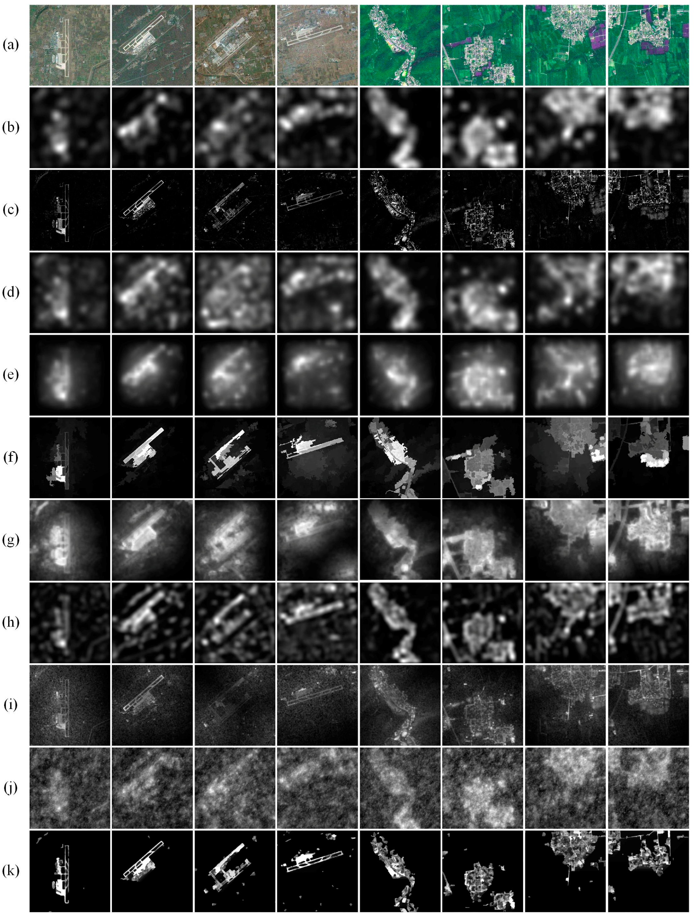
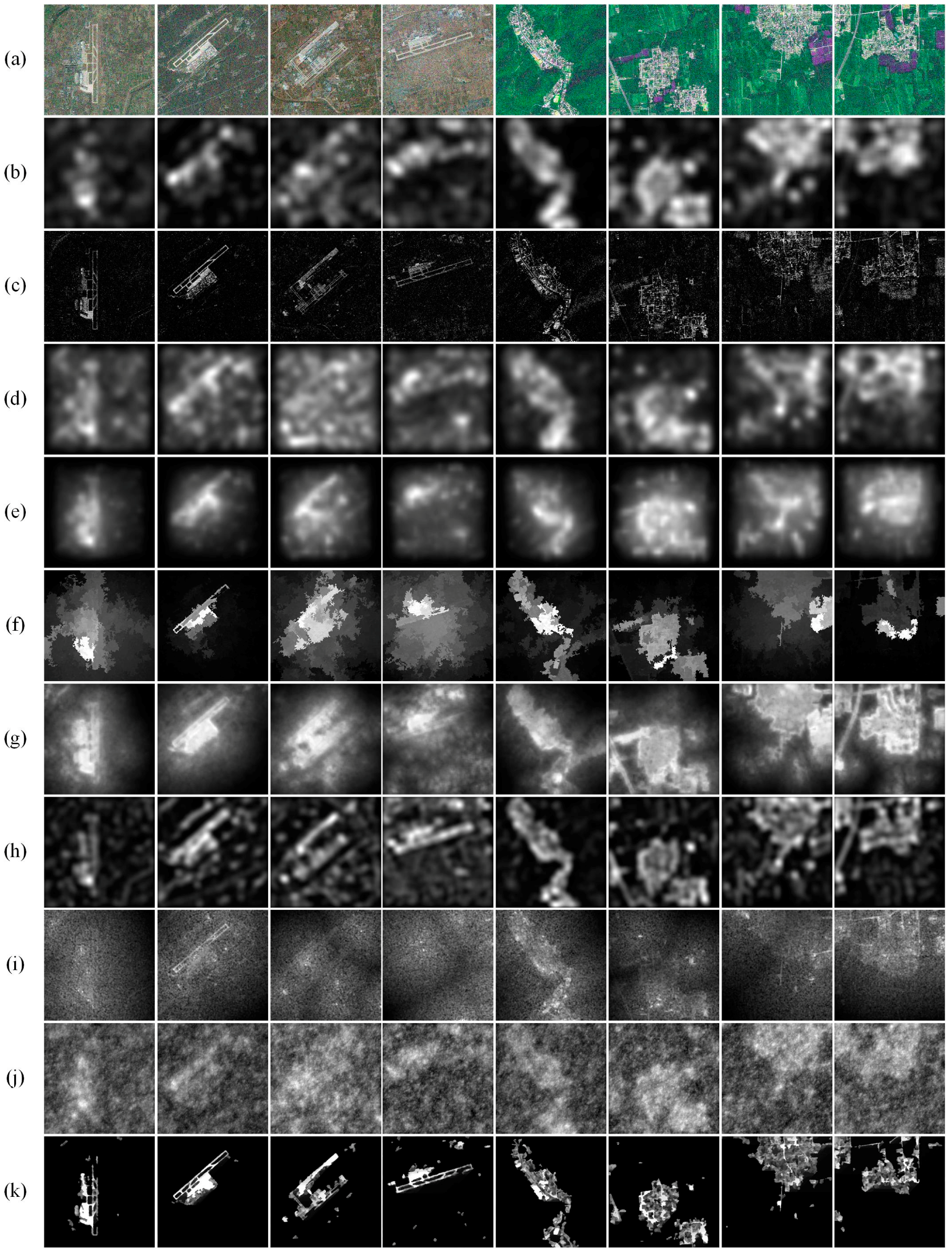
In Figure 7 and Figure 8, we can see that the LI model performs better than the nine competing models. As seen in Figure 7, the SR model, ITTI model and GBVS model generate low-resolution saliency maps. When used to extract ROIs in Figure 8, those low-resolution saliency maps need to be enlarged to full resolution, which fails to acquire well-defined boundaries and brings in background interference. Moreover, the ITTI model and GBVS model have undesirable extraction results when ROIs lie near image boundaries. The FT model puts emphasis on regions with high gradients so it can extract clear boundaries. However, as seen in Figure 8, it produces some fragments in and outside the ROIs and destroys the integrity of ROIs. The followings can also be learned from Figure 8. The H model mainly focuses on color similarity and generates well-defined boundaries, but it returns false extractions when ROIs lie near image boundaries. Airports acquired by the CA model are not intact, and residential areas acquired have some outside interference such as water mass. The FDA model cannot eliminate outside interference such as roads. The WT model detects many fragments in the background and mistakes them as ROIs. The MFF model performs well in images acquired by the SPOT 5 satellite but is not satisfactory when images are from Google Earth with more complex backgrounds. Compared with nine competing models, the LI model can not only maintain clear boundaries but also eliminate various kinds of interference such as shadows, water mass and roads to a great extent. It also guarantees the integrity of ROIs with few fragments.
3.1.2. Quantitative Comparisons
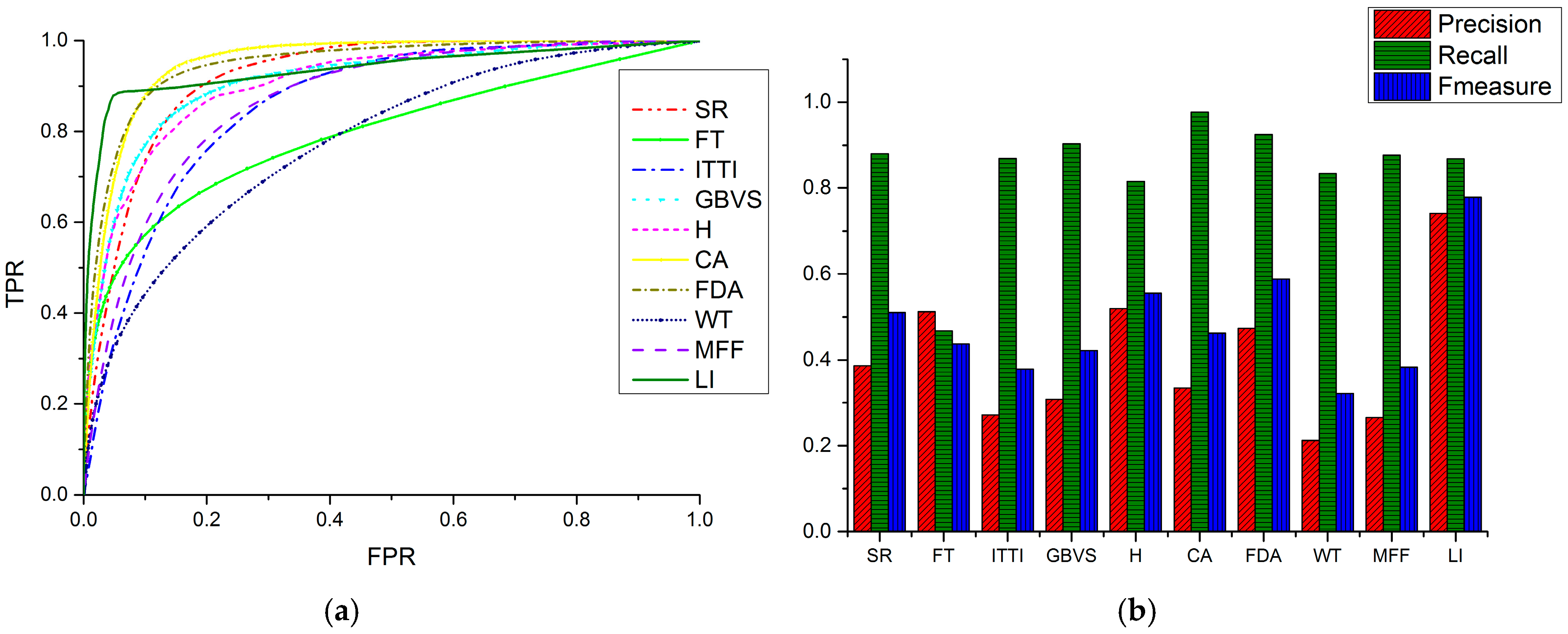
The receiver operator characteristic (ROC) curve and precision (P), recall (R) and F-measure (F) values are used to compare the performance across the ten models quantitatively. Results are shown in Figure 9.
The ROC curve is often used as a significant objective evaluation of a visual saliency model. We generate a binary image by classifying the locations in a saliency map as ROIs and non-ROIs using varying quantization thresholds. The percentage of ROIs from the ground truth intersecting with the ROIs from the binary image is called the true positive rate (TPR). The percentage of non-ROIs from the ground truth intersecting with the ROIs from the binary image is called the false positive rate (FPR). The relationships can be represented as:
where is the ground truth, and is the binary image after threshold binarization. denotes the coordinates of images.
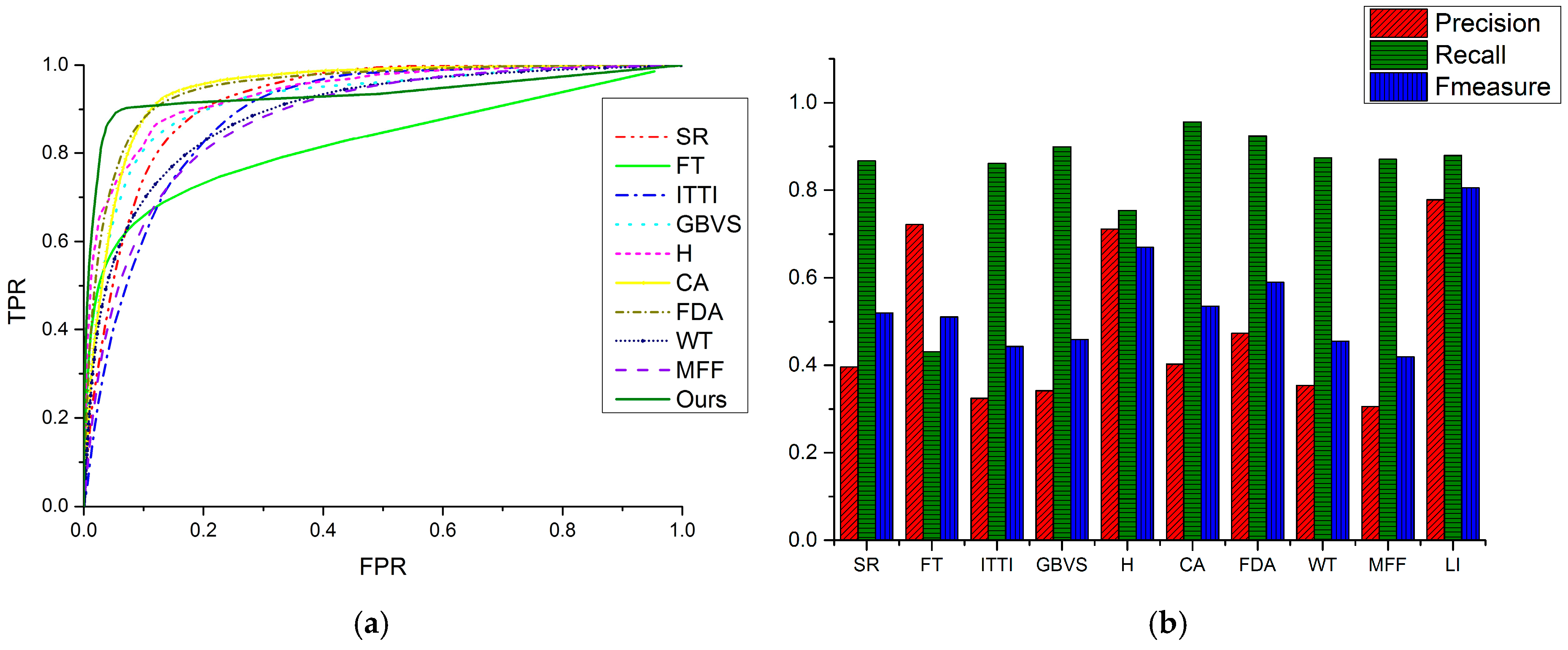
Different thresholds reflect the performance of a model in different situations. If the threshold is small, more true salient regions will be extracted, so the TPR value will be high. However, more non-salient regions will also be extracted, and thus the FPR value is increased. At the same TPR value, a lower FPR value indicates better performance. At the same FPR value, a higher TPR value indicates better performance. The ROC curve is acquired by plotting different pairs of (FPR, TPR) generated by varied thresholds. We normalize the gray values of saliency maps into [0, 1]. The threshold interval is 0.01 so that 101 thresholds are employed to generate (FPR, TPR) pairs.
Another quantitative experiment is based on precision, recall and F-measure, denoted as , and , respectively. They are defined as follows:
where is the ground truth, and is the binary image after segmentation. High recall means that a model returns most of the ROIs, whereas high precision means that a model returns substantially more ROIs than background regions. The F-measure is the harmonic mean of precision and recall. A larger weights recall higher than precision, while a smaller emphasizes precision more than recall. In our evaluation, we use , which means that precision and recall are equally important. Figure 9b is the comparison of the LI model and nine competing models in terms of precision, recall and F-measure.
In Figure 9b we can see that the LI model has the second highest precision value, which means that it can extract ROIs precisely with less interference. The FT model is slightly better than ours in terms of precision but has the lowest recall value among the ten models. The LI model has the largest recall value, meaning that it can extract the most ROIs from remote sensing images among the ten models. The value of F-measure evaluates the comprehensive ability of saliency models, and the LI model has the highest value of F-measure, which indicates that it has a better performance.
3.2. ROI Detection in Noisy Images
3.2.1. Qualitative Comparisons
We add Gaussian noise with mean of 0 and standard variance of 0.01 and 0.05 to the remote sensing images. Saliency maps and ROI detection results are shown in Figure 10, Figure 11, Figure 12 and Figure 13.
As seen from the comparisons, when images are corrupted by the Gaussian noise, all of the models perform worse than before. In general, the larger the standard variance is, the worse each model performs, which consists with our perception. Some models implicitly suppress noise by blurring and down sampling the images, such as the SR model, the ITTI model and the GBVS model. The SR model resizes the images to 64 × 64 pixels to generate low-resolution saliency maps, and the ITTI model and the GBVS model down sample the images using the Gaussian Pyramid. The down-sampling operation can alleviate the effect of noise by removing some of the noise pixels when used to generate saliency maps. The FT model can eliminate the influence of noise to some extent through Gaussian blurring in computing saliency maps. The H model shows stability when test images are acquired by the SPOT 5 satellite. For noisy Google Earth images, it cannot obtain desirable results. The CA model detects integrated ROIs but introduces more interference with the increase of the standard variance. Although the FDA model and the MFF model still detect some outside interference, they are relatively stable because the Gaussian Pyramid is used. The WT model detects many fragments and backgrounds and is unstable. The LI model can resist the effect of noise and keep clear backgrounds better because the Gaussian Pyramid is employed to perform multi-scale saliency analysis and the superpixel segmentation is not sensitive to noise.
3.2.2. Quantitative Comparisons
Figure 14 and Figure 15 are ROC curves and PRF comparisons of the ten models using noisy images with standard variance of 0.01 and 0.05. From Figure 14a and Figure 15a we obtain similar conclusions as those in Section 3.2.1. Most models are comparatively stable since most ROC curves are not significantly different from those for noise-free images. Only the curve of the WT model (colored in navy) has an explicit change, which indicates that the model is not quite stable. Figure 14b and Figure 15b show that with the increase of standard variance, the precision values of ten models decrease and the recall values slightly increase. The LI model has the largest precision value, which means that it can extract ROIs with relatively less interference when dealing with noisy images. The LI model still has the largest value of the F-measure, even when there is noise, which means that its overall performance is more stable than those of the nine competing models.
3.3. Additional Discussions
After many experiments, we find that the limitation of the LI model is that it is not suitable for low spatial resolution remote sensing images and hyperspectral remote sensing images. For low spatial resolution remote sensing images, there exist many mixed pixels that contain more than one objects in a pixel, so it is hard to distinguish different targets. Since hyperspectral remote sensing images have dozens or even hundreds of spectra, it is of great importance to choose proper spectra for experiments. However, the LI model aims at processing remote sensing images with a few spectra. When there are dozens or even hundreds of spectra, it does not consider optimizing the choice of spectra for a better detection result. Thus, its application in hyperspectral remote sensing images is limited.
The LI model is most suitable for middle and high spatial resolution remote sensing images. In middle and high resolution remote sensing images, the resolution of single spectrum increases so the spatial characteristics of spectra can be employed to improve the accuracy of target detection. The shape, texture, spectrum and other detail information is clearer and more abundant; however, the more complex backgrounds act as a big disturbance in accurate target detection. In the LI model, we take full advantage of characteristics of the panchromatic image and multi-spectrum images to perform saliency analysis, and then design a pixel-saliency-enhancement strategy to eliminate the interference in the backgrounds.
If the panchromatic image is not available in a given dataset, we can use multi-spectral images to compose a colored image and employ the grayscale version of the colored image to perform the superpixel segmentation. Then, the global spatially weighted superpixel intensity contrast is calculated for the grayscale image to acquire the intensity saliency map.
4. Conclusions
The increasing resolution of remote sensing images makes it harder to extract regions of interest (ROIs) in high-resolution remote sensing images accurately and efficiently. In this paper, we propose a novel saliency analysis and ROI extraction method for remote sensing images, which is composed of local–global contrast analysis for panchromatic images and intra-spectrum information distribution estimation (LI) for multi-spectral images. There are three major contributions in our paper: (1) for the panchromatic image, superpixels with similar size and well-defined boundaries are obtained by segmentation and then treated as basic processing units to compute the intensity saliency map; (2) for multi-spectral images, we exploit their information complementarity to the panchromatic image and introduce the information theory to calculate the spectrum saliency map; and (3) a pixel-level saliency enhancement strategy is presented to highlight the salient objects and suppress the non-salient objects. Experiments were conducted using images from the SPOT 5 satellite and Google Earth. The results show that the LI model is better than nine competing models in terms of both quality and quantity and is stable when faced with noisy images.
Acknowledgments
This work was supported by the National Natural Science Foundation of China under grant number 61571050; the Beijing Natural Science Foundation under grant number 4162033; and the Open Fund of State Key Laboratory of Remote Sensing Science under grant number OFSLRSS201621.
Author Contributions
Libao Zhang and Shiyi Wang had the original idea for the study; Libao Zhang supervised the research and contributed to the article’s organization; Libao Zhang conceived and designed the experiments; Shiyi Wang performed the experiments; Libao Zhang and Shiyi Wang analyzed the data; and Libao Zhang and Shiyi Wang wrote the paper. All authors read and approved the submitted manuscript.
Conflicts of Interest
The authors declare no conflict of interest.
References
- Brinkmann, R. The Art and Science of Digital Compositing, 2nd ed.; Morgan Kaufmann: San Mateo, CA, USA, 1999; p. 184. [Google Scholar]
- Zhang, L.; Chen, J.; Qiu, B. Region-of-interest coding based on saliency detection and directional wavelet for remote sensing images. IEEE Geosci. Remote Sens. Lett. 2017, 14, 23–27. [Google Scholar] [CrossRef]
- Chen, J.; Zhang, L. Joint Multi-Image Saliency Analysis for Region of Interest Detection in Optical Multispectral Remote Sensing Images. Remote Sens. 2016, 8, 461. [Google Scholar] [CrossRef]
- Zhu, D.; Wang, B.; Zhang, L. Airport target detection in remote sensing images: A new method based on two-way saliency. IEEE Geosci. Remote Sens. Lett. 2015, 12, 1096–1100. [Google Scholar]
- Xu, F.; Liu, J.; Sun, M.; Zeng, D.; Wang, X. A Hierarchical Maritime Target Detection Method for Optical Remote Sensing Imagery. Remote Sens. 2017, 9, 280. [Google Scholar] [CrossRef]
- Huang, X.; Yang, W.; Zhang, H.; Xia, G. Automatic Ship Detection in SAR Images Using Multi-Scale Heterogeneities and an A Contrario Decision. Remote Sens. 2015, 7, 7695–7711. [Google Scholar] [CrossRef]
- Hu, J.; Xia, G.; Hu, F.; Zhang, L. A Comparative Study of Sampling Analysis in the Scene Classification of Optical High-Spatial Resolution Remote Sensing Imagery. Remote Sens. 2015, 7, 14988–15013. [Google Scholar] [CrossRef]
- Arvor, D.; Durieux, L.; Andrés, S.; Laporte, M. Advances in geographic object-based image analysis with ontologies: A review of main contributions and limitations from a remote sensing perspective. ISPRS J. Photogramm. Remote Sens. 2013, 82, 125–137. [Google Scholar] [CrossRef]
- Zhong, Y.; Zhao, J.; Zhang, L. A hybrid object-oriented conditional random field classification framework for high spatial resolution remote sensing imagery. IEEE Trans. Geosci. Remote Sens. 2014, 52, 7023–7037. [Google Scholar] [CrossRef]
- Zhang, L.; Li, A.; Zhang, Z.; Yang, K. Global and local saliency analysis for the extraction of residential areas in high-spatial-resolution remote sensing image. IEEE Trans. Geosci. Remote Sens. 2016, 54, 3750–3763. [Google Scholar] [CrossRef]
- Zhao, Q.; Koch, C. Learning saliency-based visual attention: A review. Signal Process. 2013, 93, 1401–1407. [Google Scholar] [CrossRef]
- Borji, A.; Cheng, M.; Jiang, H.; Li, J. Salient object detection: A benchmark. IEEE Trans. Image Process. 2015, 24, 5706–5722. [Google Scholar] [CrossRef] [PubMed]
- Koch, C.; Ullman, S. Shifts in selective visual attention: Towards the underlying neural circuitry. Hum. Neurobiol. 1985, 4, 219–227. [Google Scholar] [PubMed]
- Itti, L.; Koch, C.; Niebur, E. A model of saliency-based visual attention for rapid scene analysis. IEEE Trans. Pattern Anal. Mach. Intell. 1998, 20, 1254–1259. [Google Scholar] [CrossRef]
- Goferman, S.; Zelnik-Manor, L.; Tal, A. Context-aware saliency detection. IEEE Trans. Pattern Anal. Mach. Intell. 2012, 34, 1915–1926. [Google Scholar] [CrossRef] [PubMed]
- le Meur, O.; le Callet, P.; Barba, D.; Thoreau, D. A coherent computational approach to model bottom-up visual attention. IEEE Trans. Pattern Anal. Mach. Intell. 2006, 28, 802–817. [Google Scholar] [CrossRef] [PubMed]
- Ma, Y.; Zhang, H. Contrast-Based Image Attention Analysis by Using Fuzzy Growing. In Proceedings of the Eleventh ACM International Conference on Multimedia, Berkeley, CA, USA, 2–8 November 2003; ACM: New York, NY, USA, 2003; pp. 374–381. [Google Scholar]
- Zhang, L.; Chen, J.; Qiu, B. Region of interest extraction in remote sensing images by saliency analysis with the normal directional lifting wavelet transform. Neurocomputing 2016, 179, 186–201. [Google Scholar] [CrossRef]
- Bruce, N.; Tsotsos, J. Saliency based on information maximization. In Advances in Neural Information Processing Systems; MIT Press: Cambridge, MA, USA, 2005; pp. 155–162. [Google Scholar]
- Cheng, M.; Zhang, G.; Mitra, N.J.; Huang, X.; Hu, S. Global contrast based salient region detection. In Proceedings of the IEEE Conference on Computer Vision and Pattern Recognition, Providence, RI, USA, 20–25 June 2011; pp. 409–416. [Google Scholar]
- Hou, X.; Zhang, L. Saliency detection: A spectral residual approach. In Proceedings of the IEEE Conference on Computer Vision and Pattern Recognition, Minneapolis, MN, USA, 18–23 June 2007; pp. 1–8. [Google Scholar]
- Imamoglu, N.; Lin, W.; Fang, Y. A saliency detection model using low-level features based on wavelet transform. IEEE Trans. Multimed. 2013, 15, 96–105. [Google Scholar] [CrossRef]
- Rosin, P.L. A simple method for detecting salient regions. Pattern Recognit. 2009, 42, 2363–2371. [Google Scholar] [CrossRef]
- Harel, J.; Koch, C.; Perona, P. Graph-based visual saliency. Neural Inf. Proc. Syst. 2006, 19, 545–552. [Google Scholar]
- Achanta, R.; Hemami, S.; Estrada, F.; Susstrunk, S. Frequency-tuned salient region detection. In Proceedings of the IEEE Conference on Computer Vision and Pattern Recognition, Miami, FL, USA, 20–25 June 2009; pp. 1597–1604. [Google Scholar]
- Shi, J.; Yan, Q.; Xu, L.; Jia, J. Hierarchical image saliency detection on extended CSSD. IEEE Trans. Pattern Anal. Mach. Intell. 2016, 38, 717–729. [Google Scholar] [CrossRef] [PubMed]
- Cheng, M.; Mitra, N.; Huang, X.; Torr, P.; Hu, S. Global contrast based salient region detection. IEEE Trans. Pattern Anal. Mach. Intell. 2015, 37, 569–582. [Google Scholar] [CrossRef] [PubMed]
- Ren, X.; Malik, J. Learning a classification model for segmentation. In Proceedings of the Ninth IEEE International Conference on Computer Vision; IEEE Computer Society: Washington, DC, USA, 2003; pp. 10–17. [Google Scholar]
- Levinshtein, A.; Stere, A.; Kutulakos, K.N.; Fleet, D.J.; Dickinson, S.J.; Siddiqi, K. TurboPixels: Fast superpixels using geometric flows. IEEE Trans. Pattern Anal. Mach. Intell. 2009, 31, 2290–2297. [Google Scholar] [CrossRef] [PubMed]
- Borji, A. What is a salient object? A dataset and a baseline model for salient object detection. IEEE Trans. Image Process. 2015, 24, 742–756. [Google Scholar] [CrossRef] [PubMed]
- Guo, C.; Zhang, L. A novel multiresolution spatiotemporal saliency detection model and its applications in image and video compression. IEEE Trans. Image Process. 2010, 19, 185–198. [Google Scholar] [PubMed]
- Dong, Y.; Pourazad, M.T.; Nasiopoulos, P. Human visual system-based saliency detection for high dynamic range content. IEEE Trans. Multimed. 2016, 18, 549–562. [Google Scholar] [CrossRef]
- Yang, K.; Gao, S.; Li, C.; Li, Y. Efficient Color Boundary Detection with Color-Opponent Mechanisms. In Proceedings of the IEEE Conference on Computer Vision and Pattern Recognition, Columbus, OH, USA, 23–27 June 2013; pp. 2810–2817. [Google Scholar]
- Moan, S.L.; Mansouri, A.; Hardeberg, J.Y.; Voisin, Y. Saliency for spectral image analysis. IEEE J. Sel. Top. Appl. Earth Obs. Remote Sens. 2013, 6, 2472–2478. [Google Scholar] [CrossRef]
- Zhang, L.; Sun, Q.; Chen, J. Multi-Image Saliency Analysis via Histogram and Spectral Feature Clustering for Satellite Images. In Proceedings of the 2016 IEEE International Conference on Image Processing, Phoenix, AZ, USA, 25–28 September 2016; pp. 2802–2806. [Google Scholar]
- Wang, S.; Fu, Y.; Xing, K.; Han, X. A Model of Target Recognition from Remote Sensing Images. In Proceedings of the 2009 IEEE/RSJ International Conference on Intelligent Robots and Systems, St. Louis, MO, USA, 10–15 October 2009; pp. 3665–3670. [Google Scholar]
- Zhang, L.; Yang, K.; Li, H. Regions of interest detection in panchromatic remote sensing images based on multiscale feature fusion. IEEE J. Sel. Top. Appl. Earth Obs. Remote Sens. 2014, 7, 4704–4716. [Google Scholar] [CrossRef]
- Zhang, L.; Yang, K. Region-of-interest extraction based on frequency domain analysis and salient region detection for remote sensing image. IEEE Geosci. Remote Sens. Lett. 2014, 11, 916–920. [Google Scholar] [CrossRef]
- Otsu, N. A Threshold Selection Method from Gray-Level Histograms. IEEE Trans. Syst. Man Cyber. 1979, 9, 62–66. [Google Scholar] [CrossRef]
- Gonzalo-Martín, C.; Lillo-Saavedra, M.; Menasalvas, E.; Fonseca-Luengo, D.; García-Pedrero, A.; Costumero, R. Local optimal scale in a hierarchical segmentation method for satellite images. J. Intell. Inf. Syst. 2016, 46, 517–529. [Google Scholar] [CrossRef]
- Garcia-Pedrero, A.; Gonzalo-Martin, C.; Fonseca-Luengo, D.; Lillo-Saavedra, M. A GEOBIA methodology for fragmented agricultural landscapes. Remote Sens. 2015, 7, 767–787. [Google Scholar] [CrossRef]
- Siddiqi, K.; Bouix, S.; Tannenbaum, A.; Zucker, S. Hamilton-jacobi skeletons. Int. J. Comput. Vis. 2002, 48, 215–231. [Google Scholar] [CrossRef]
- Perazzi, F.; Krahenb, P.; Pritch, Y. Saliency Filters: Contrast Based Filtering for Salient Region Detection. In Proceedings of the IEEE Conference on Computer Vision and Pattern Recognition, Providence, RL, USA, 16–21 June 2012; pp. 733–740. [Google Scholar]
- Wang, K.; Lin, L.; Lu, J.; Li, C.; Shi, K. PISA: Pixelwise image saliency by aggregating complementary appearance contrast measures with edge-preserving coherence. IEEE Trans. Image Process. 2015, 24, 3019–3033. [Google Scholar] [CrossRef] [PubMed]
- Ma, L.; Du, B.; Soomro, N.Q. Region-of-interest detection via superpixel-to-pixel saliency analysis for remote sensing image. IEEE Geosci. Remote Sens. Lett. 2016, 13, 1752–1756. [Google Scholar] [CrossRef]
- Kannan, R.; Ghinea, G.; Swaminathan, S. Salient region detection using patch level and region level image abstractions. IEEE Signal Process. Lett. 2015, 22, 686–690. [Google Scholar] [CrossRef]
Figure 1.
The framework of the LI mode: (a) superpixel segmentation; (b) saliency analysis; and (c) saliency enhancement and region of interest (ROI) extraction.
Figure 1.
The framework of the LI mode: (a) superpixel segmentation; (b) saliency analysis; and (c) saliency enhancement and region of interest (ROI) extraction.

Figure 2.
Segmentation steps and the result.
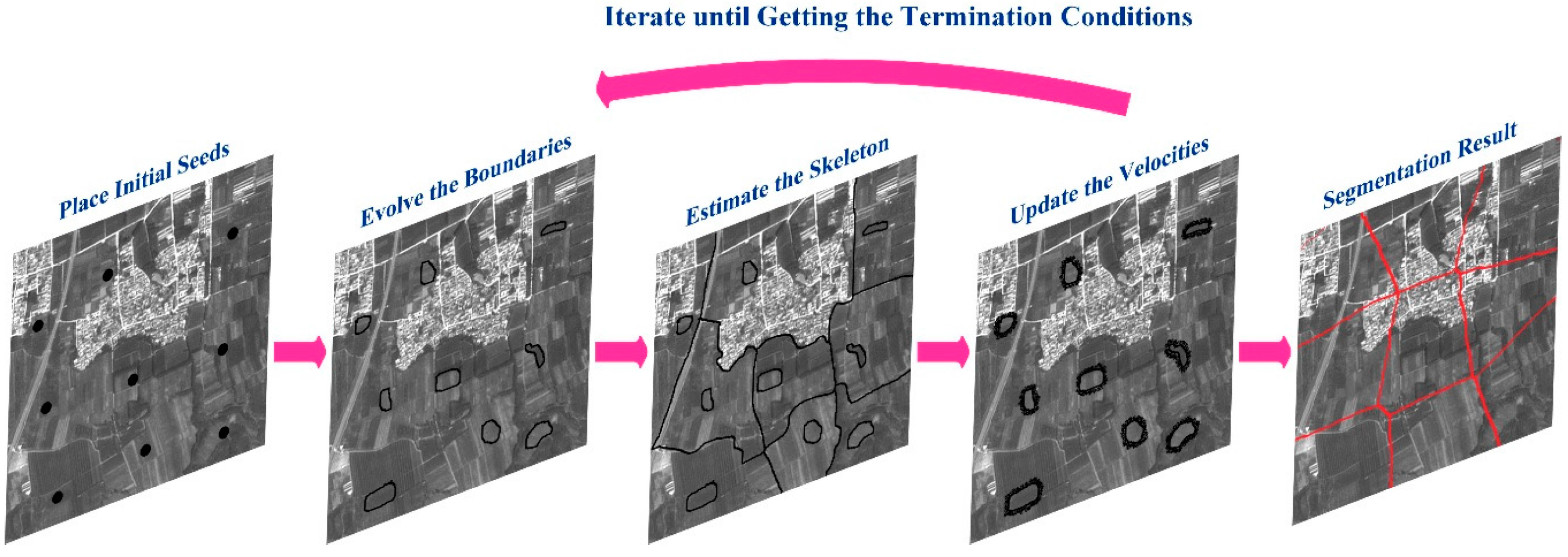
Figure 3.
Information saliency maps and spectrum saliency maps: (a) information saliency maps; (b) spectrum saliency maps.
Figure 3.
Information saliency maps and spectrum saliency maps: (a) information saliency maps; (b) spectrum saliency maps.

Figure 4.
Intra-spectrum information distribution estimation.

Figure 5.
Comparison of saliency maps before and after the saliency enhancement: (a) saliency maps before the saliency enhancement; and (b) saliency maps after the saliency enhancement.
Figure 5.
Comparison of saliency maps before and after the saliency enhancement: (a) saliency maps before the saliency enhancement; and (b) saliency maps after the saliency enhancement.
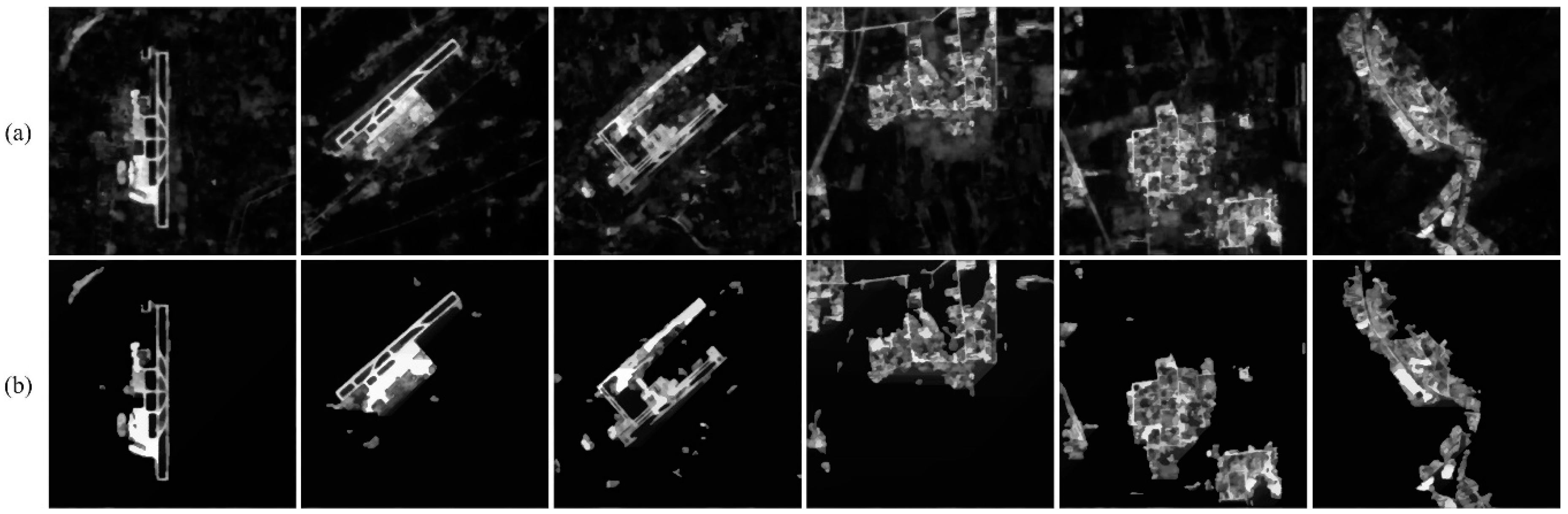
Figure 6.
Saliency enhancement and ROI extraction.
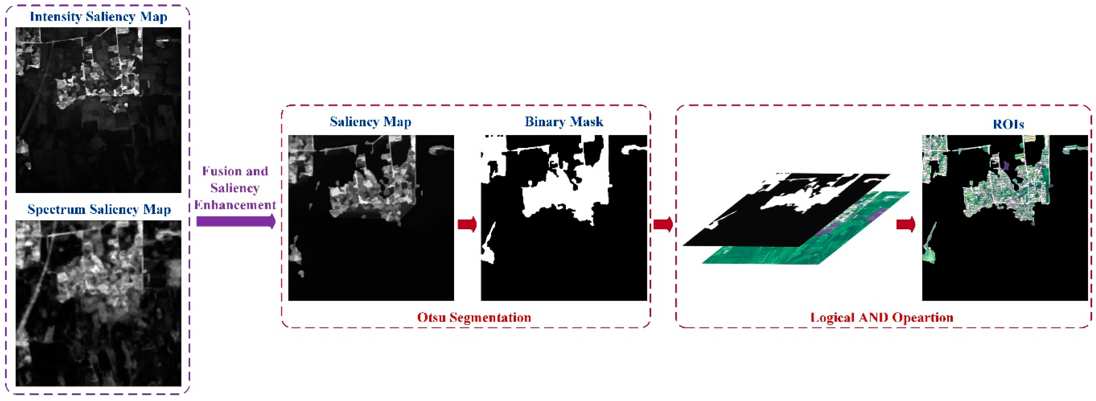
Figure 7.
Comparison of saliency maps for noise-free images (first four images are from the SPOT5 satellite and last four are from Google Earth): (a) remote sensing image; (b) SR; (c) FT; (d) ITTI; (e) GBVS; (f) H; (g) CA; (h) FDA; (i) WT; (j) MFF; and (k) LI.
Figure 7.
Comparison of saliency maps for noise-free images (first four images are from the SPOT5 satellite and last four are from Google Earth): (a) remote sensing image; (b) SR; (c) FT; (d) ITTI; (e) GBVS; (f) H; (g) CA; (h) FDA; (i) WT; (j) MFF; and (k) LI.
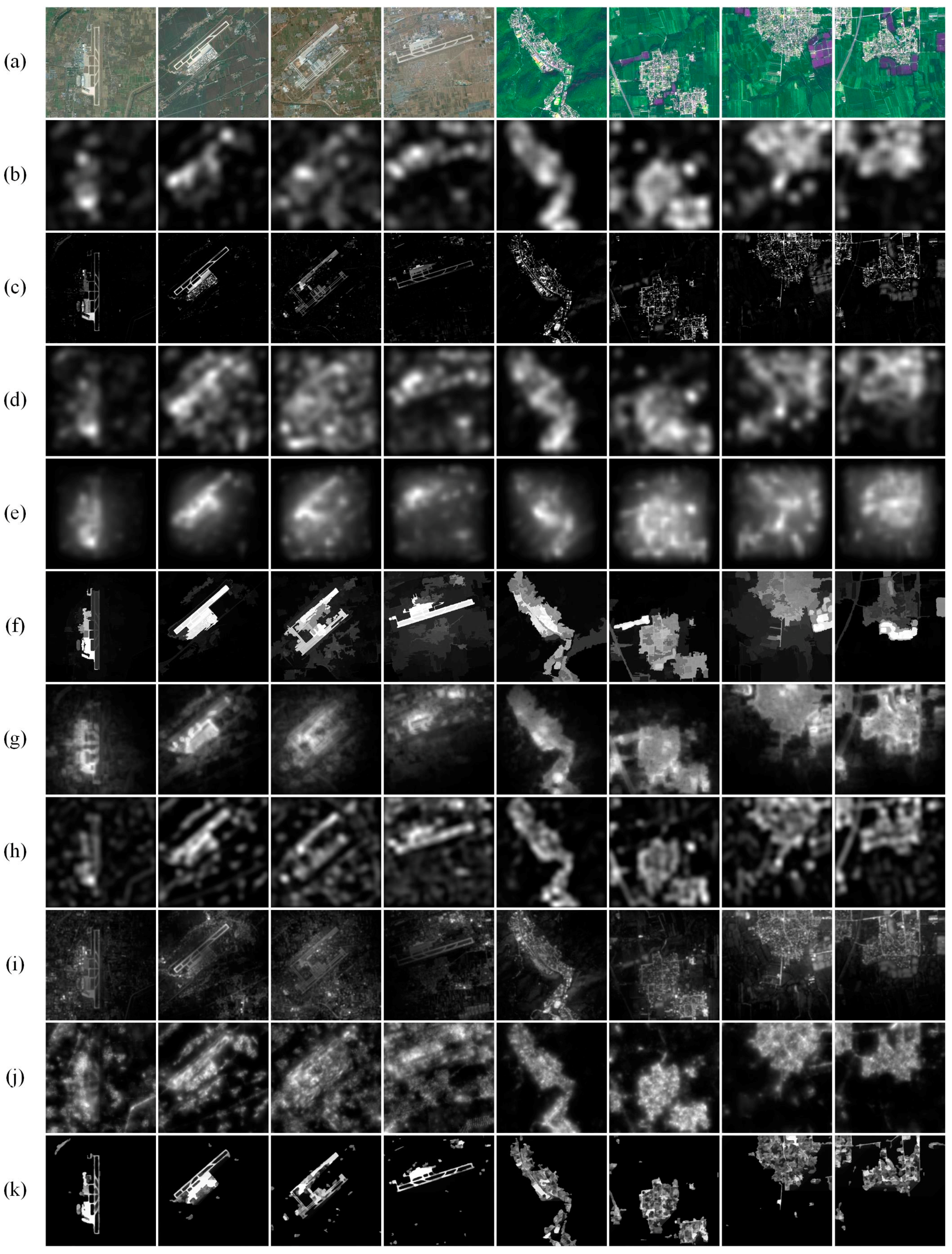
Figure 8.
Comparison of ROIs for noise-free images (first four images are from the SPOT5 satellite and last four are from Google Earth): (a) ground truth; (b) SR; (c) FT; (d) ITTI; (e) GBVS; (f) H; (g) CA; (h) FDA; (i) WT; (j) MFF; and (k) LI.
Figure 8.
Comparison of ROIs for noise-free images (first four images are from the SPOT5 satellite and last four are from Google Earth): (a) ground truth; (b) SR; (c) FT; (d) ITTI; (e) GBVS; (f) H; (g) CA; (h) FDA; (i) WT; (j) MFF; and (k) LI.
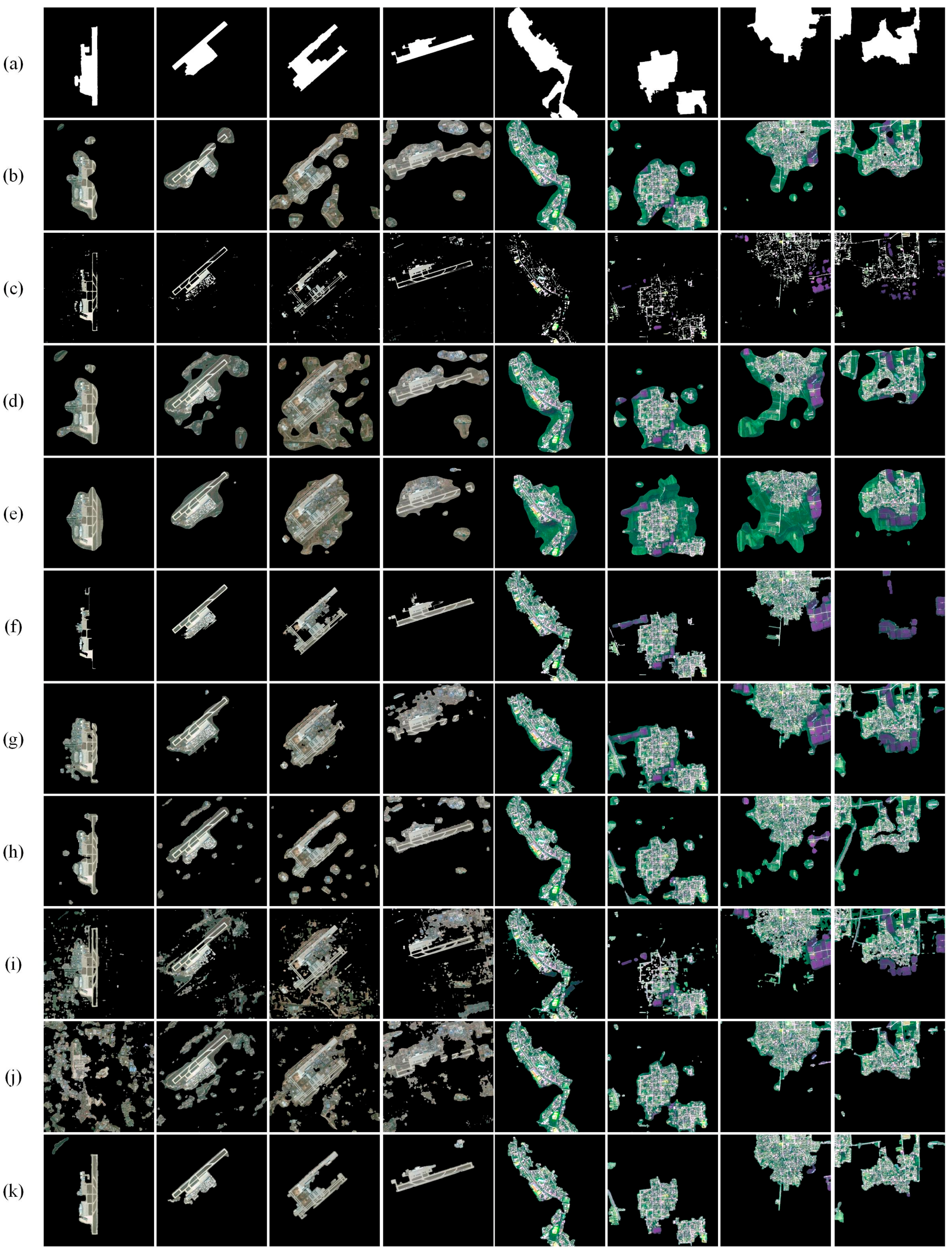
Figure 9.
Quantitative comparisons for noise-free images: (a) Receiver operator characteristic (ROC) curves; and (b) Precision, recall and F-measure (PRF) values.
Figure 9.
Quantitative comparisons for noise-free images: (a) Receiver operator characteristic (ROC) curves; and (b) Precision, recall and F-measure (PRF) values.
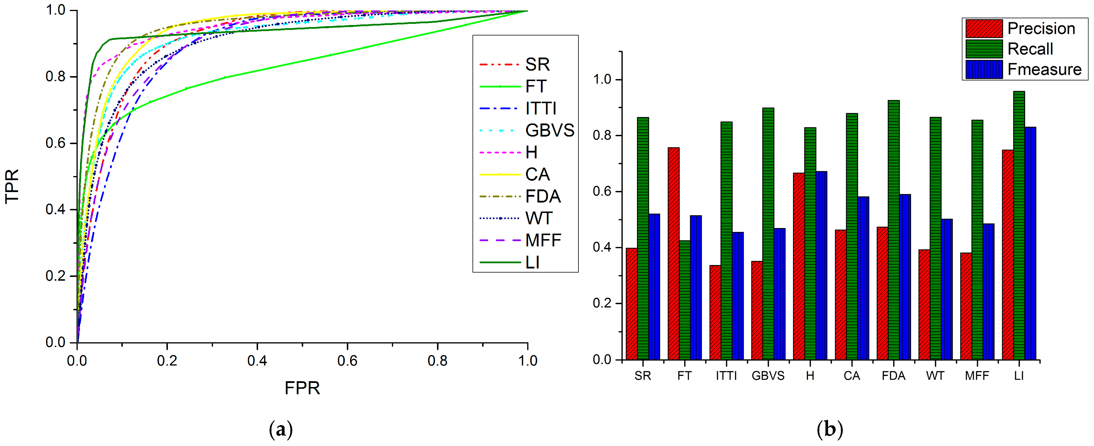
Figure 10.
Comparison of saliency maps for images polluted by Gaussian noise (Standard Variance = 0.01) (first four images are from the SPOT5 satellite and last four are from Google Earth): (a) remote sensing image; (b) SR; (c) FT; (d) ITTI; (e) GBVS; (f) H; (g) CA; (h) FDA; (i) WT; (j) MFF; and (k) LI.

Figure 11.
Comparison of ROIs for images polluted by Gaussian noise (Standard Variance = 0.01) (first four images are from the SPOT5 satellite and last four are from Google Earth): (a) ground truth; (b) SR; (c) FT; (d) ITTI; (e) GBVS; (f) H; (g) CA; (h) FDA; (i) WT; (j) MFF; and (k) LI.
Figure 11.
Comparison of ROIs for images polluted by Gaussian noise (Standard Variance = 0.01) (first four images are from the SPOT5 satellite and last four are from Google Earth): (a) ground truth; (b) SR; (c) FT; (d) ITTI; (e) GBVS; (f) H; (g) CA; (h) FDA; (i) WT; (j) MFF; and (k) LI.
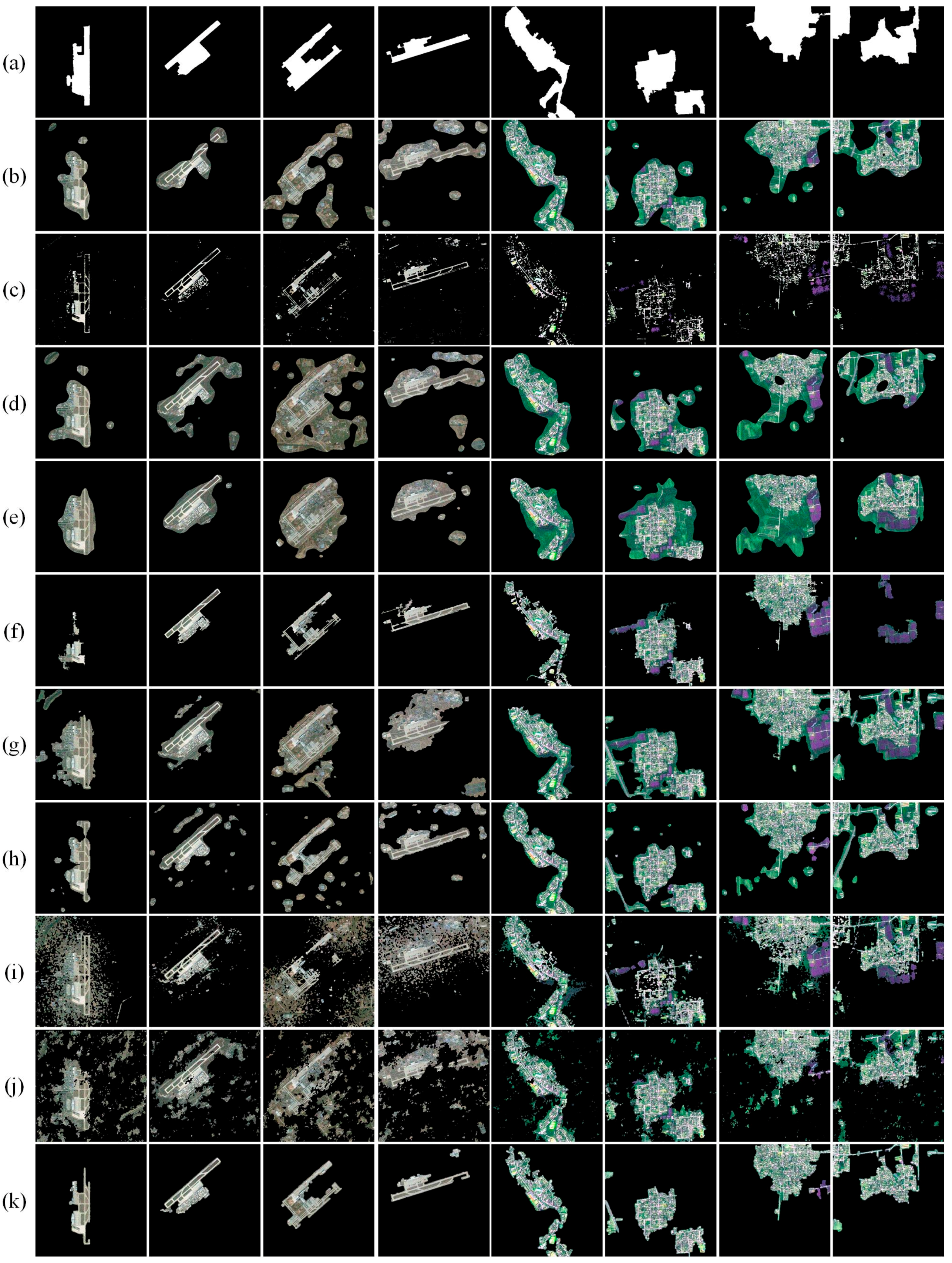
Figure 12.
Comparison of saliency maps for images polluted by Gaussian noise (Standard Variance = 0.05) (first four images are from the SPOT5 satellite and last four are from Google Earth): (a) remote sensing image; (b) SR; (c) FT; (d) ITTI; (e) GBVS; (f) H; (g) CA; (h) FDA; (i) WT; (j) MFF; and (k) LI.

Figure 13.
Comparison of ROIs for images polluted by Gaussian noise (Standard Variance = 0.05) (first four images are from the SPOT5 satellite and last four are from Google Earth): (a) ground truth; (b) SR; (c) FT; (d) ITTI; (e) GBVS; (f) H; (g) CA; (h) FDA; (i) WT; (j) MFF; and (k) LI.
Figure 13.
Comparison of ROIs for images polluted by Gaussian noise (Standard Variance = 0.05) (first four images are from the SPOT5 satellite and last four are from Google Earth): (a) ground truth; (b) SR; (c) FT; (d) ITTI; (e) GBVS; (f) H; (g) CA; (h) FDA; (i) WT; (j) MFF; and (k) LI.
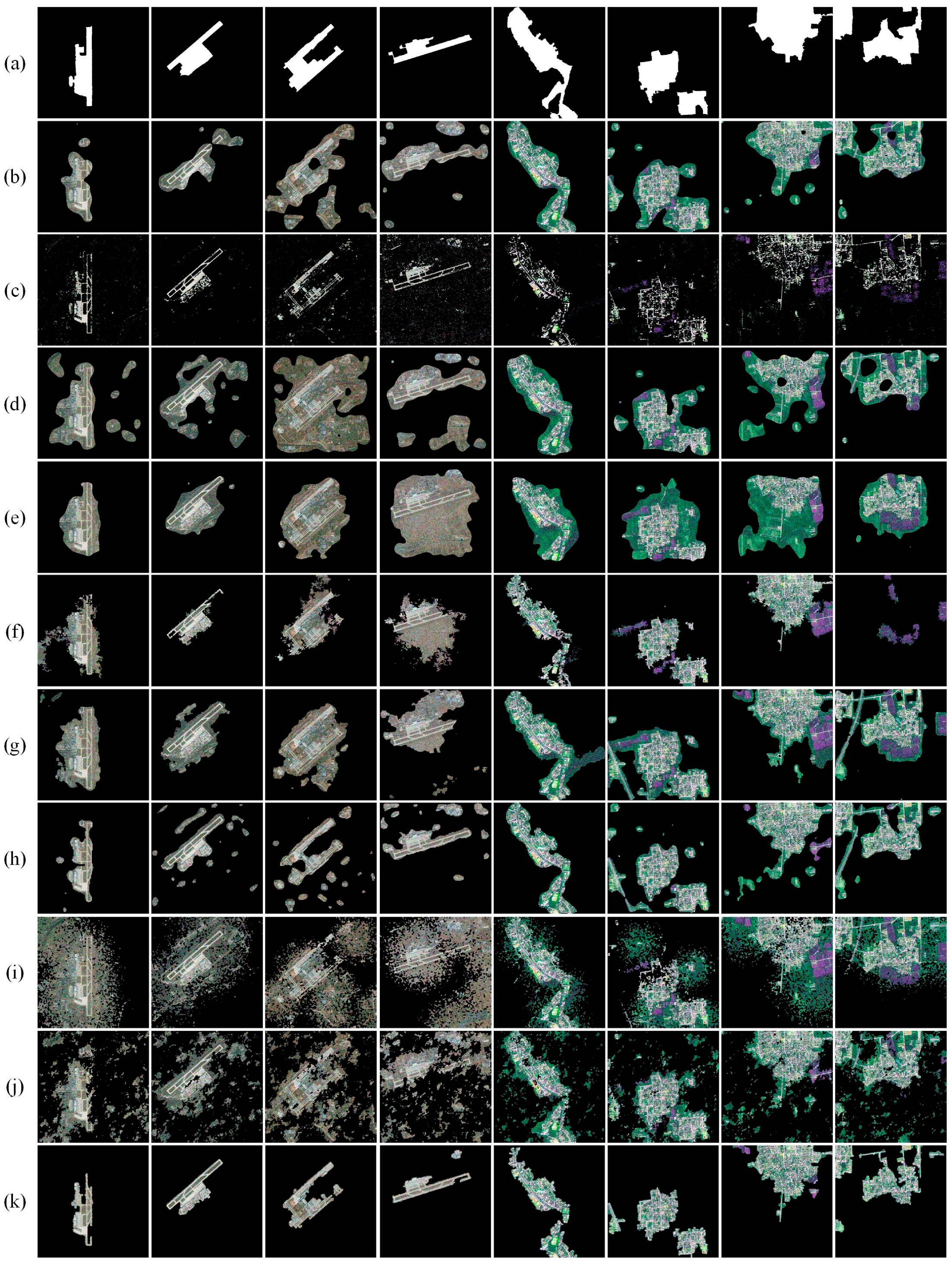
Figure 14.
Quantitative comparisons for images polluted by Gaussian noise (Standard Variance = 0.01). (a) ROC curves; (b) PRF values.
Figure 14.
Quantitative comparisons for images polluted by Gaussian noise (Standard Variance = 0.01). (a) ROC curves; (b) PRF values.

Figure 15.
Quantitative comparisons for images polluted by Gaussian noise (Standard Variance = 0.05): (a) ROC curves; and (b) PRF values.
Figure 15.
Quantitative comparisons for images polluted by Gaussian noise (Standard Variance = 0.05): (a) ROC curves; and (b) PRF values.
© 2017 by the authors. Licensee MDPI, Basel, Switzerland. This article is an open access article distributed under the terms and conditions of the Creative Commons Attribution (CC BY) license (http://creativecommons.org/licenses/by/4.0/).
Share and Cite
MDPI and ACS Style
Zhang, L.; Wang, S. Region-of-Interest Extraction Based on Local–Global Contrast Analysis and Intra-Spectrum Information Distribution Estimation for Remote Sensing Images. Remote Sens. 2017, 9, 597. https://doi.org/10.3390/rs9060597
AMA Style
Zhang L, Wang S. Region-of-Interest Extraction Based on Local–Global Contrast Analysis and Intra-Spectrum Information Distribution Estimation for Remote Sensing Images. Remote Sensing. 2017; 9(6):597. https://doi.org/10.3390/rs9060597
Chicago/Turabian StyleZhang, Libao, and Shiyi Wang. 2017. "Region-of-Interest Extraction Based on Local–Global Contrast Analysis and Intra-Spectrum Information Distribution Estimation for Remote Sensing Images" Remote Sensing 9, no. 6: 597. https://doi.org/10.3390/rs9060597
Note that from the first issue of 2016, this journal uses article numbers instead of page numbers. See further details here.