
Comparison of Three Theoretical Methods for Determining Dry and Wet Edges of the LST/FVC Space: Revisit of Method Physics


College of Geoscience and Surveying Engineering, China University of Mining and Technology, Beijing 100083, China
*
Author to whom correspondence should be addressed.
Remote Sens. 2017, 9(6), 528; https://doi.org/10.3390/rs9060528
Submission received: 10 April 2017
/
Revised: 17 May 2017
/
Accepted: 24 May 2017
/
Published: 26 May 2017
Abstract
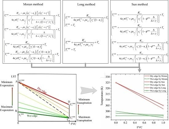
:Land surface temperature and fractional vegetation coverage (LST/FVC) space is a classical model for estimating evapotranspiration, soil moisture, and drought monitoring based on remote sensing. One of the key issues in its utilization is to determine its boundaries, i.e., the dry and wet edges. In this study, we revisited and compared three methods that were presented by Moran et al. (1994), Long et al. (2012), and Sun (2016) for calculating the dry and wet edges theoretically. Results demonstrated that: (1) for the dry edge, the Sun method is equal to the Long method and they have greater vegetation temperature than that of the Moran method. (2) With respect to the wet edge, there are greater differences among the three methods. Generally, Long’s wet edge is a horizontal line equaling air temperature. Sun’s wet edge is an oblique line and is higher than that of the Long’s. Moran’s wet edge intersects them with a higher soil temperature and a lower vegetation temperature. (3) The Sun and Long methods are simpler in calculation and can circumvent some complex parameters as compared with the Moran method. Moreover, they outperformed the Moran method in a comparison of estimating latent heat flux (LE), where determination coefficients varied between 0.45 ~ 0.66 (Sun), 0.47 ~ 0.68 (Long), and 0.39 ~ 0.57 (Moran) among field stations.
1. Introduction
Heat energy and water vapor that are required for atmospheric motion come mainly from the land surface. Moreover, land surface heat and momentum fluxes also determine the strength and stability of turbulence and diffusion in the boundary layer as well as control the wind, temperature, and humidity changes. Consequently, land surface heat and water budget play a significant role in regional and global climate. Remote sensing is very promising in studying land surface heat and water budget since it provides a relatively cheap and rapid way to obtain up-to-date information of land surface evapotranspiration (ET), temperature, and soil moisture over a large geographical area [1].
Many methods for estimating ET and soil moisture based on remote sensing data were developed, such as SEBI (Surface Energy Balance Index) [2], SEBAL (Surface Energy Balance Algorithm for Land) [3], METRIC (Mapping EvapoTranspiration at high Resolution with Internalized Calibration) [4], a thermal inertia model for soil moisture [5], and so on. Reviews about these methods can be found [6,7,8]. However, developing a method that can avoid complex parameterization of aerodynamic and surface resistances for water and heat transfer and can enable the estimation using a remote sensing image without additional information is still a challenge [9,10,11]. Currently, the models based on Land Surface Temperature and Fractional Vegetation Coverage (LST/FVC) space show the prospect of a wide application to meet the challenge and, therefore, are of continuous interest to the remote sensing community [11,12,13,14]. One key advantage of such LST/FVC space-based methods is their simplicity in terms of their implementation, as well as the requirement of easily obtained parameters from remote sensing data. Moreover, those methods also include all the advantages of both the optical and thermal infrared methods [8] such as providing fine spatial and temporal resolution, use of relatively mature technology, long historical data, etc. In addition, the LST/FVC space is also a classical model for drought monitoring based on remote sensing. Temperature Vegetation Drought Index (TVDI) [15] and the Vegetation Temperature Condition Index (VTCI) [16] are two typical drought indexes based on the LST/FVC model.
However, one fatal drawback of such LST/FVC space-based methods is their determination of theoretical boundaries of LST/FVC space, i.e., the dry and wet edges. Generally, there are three ways to solve this issue: visual recognition, automatic fitting, and theoretical calculation. The visual recognition way is easy to implement but relies on expert’s experience, thus, it is too subjective with large uncertainties. The automatic fitting way determines the boundaries directly from remote sensing images and reduces the subjectivity and uncertainty of the visual recognition method [10]. However, this method relies on the study area generating the LST/FVC spaces. In order to achieve a satisfactory effect, it requires the study area to have areas of extreme dry and wet as well as areas with full vegetation and bare surfaces. In addition, the above two ways generally suffer from all the characteristics of an empirically derived methodology, e.g., lack of transferability to other regions, fine-tuning, and weakness to describe physical processes. Conversely, theoretical calculation derives the boundaries from an energy balance equation of land surface and, thus, allows the determination of dry and wet edges independently from the study area [17,18,19,20]. Although some parameters that are not easy to obtain by remote sensing are still necessary, the theoretical calculation method facilitates understanding the physical meanings and influence factors of dry and wet edges. Moreover, it facilitates finding a way in the future for combining the advantages of the above methods such as the objectivity and independency of the theoretical way and the simplicity and parameter accessibility of the automatic fitting way. In summary, as an objective and independent method, the theoretical calculation method is worthy of further study.
Currently, there are three typical methods belonging to the theoretical calculation method. They were, respectively, proposed by Moran et al. in 1994 [21], Long et al. in 2012 [18], and Sun Hao in 2016 [19]. In this study, the three methods are called Moran method, Long method, and Sun method for short. The three typical methods were presented with different deduction processes and expressions, which means they are hard to understand and they are limited in their application and further improvement. In addition, there is very limited research that compares them in determining the dry and wet edges or in estimating latent heat flux (LE). Motivated by the significance and potential of theoretical calculation, the aims of this study are to compare the three typical theoretical calculation methods, revisiting their basic physics, and clarify their differences and relations.
2. Revisiting the Theoretical Methods
2.1. Dry and Wet Edges
Figure 1 shows the schematic diagram of the dry and wet edges in a LST/FVC space. Points A and D represent the soil and vegetation components with the maximum water stress, respectively. Points B and C represent the soil and vegetation components with saturated water supply, respectively. Lines within the LST/FVC space are isopiestic lines of soil moisture availability [11,18]. Line BC is the wet edge and AC is the dry edge. Most research supposes the dry and wet edges as a straight line [11,13]. Following this assumption, to determine the dry and wet edges we only require the determination of LST over points A (), B (), C (), and D ().
According to the physical meanings of the dry and wet edges, their theoretical expressions can be derived from the Energy Balance Equation:
where is the net downward radiative flux (W/m2); is the downward ground heat flux into the subsurface (W/m2); is the upward surface sensible heat flux (W/m2); and is the upward surface latent heat flux (W/m2). Generally, , , and are determined by the following equation:
where and are land surface albedo and emissivity (unitless); is the down-welling shortwave radiation (W/m2); is atmosphere emissivity which can be determined using the method provided in [22]; is a constant with a value of 5.67 × 10⁻⁸ W/m2/K4; is a fraction coefficient (unitless); is the air density (kg/m3); is the specific heat of air at constant pressure (J/kg/K); is the aerodynamic resistance (s/m); and is the air temperature (K).
For bare soil and full-cover vegetation canopy components, Formula (2) has different expressions. For bare soil, we have the following formula:
where the subscript represents the parameters of the bare soil component; is the bare soil surface temperature; is aerodynamic resistance above the bare soil surface.
For the full-cover vegetation canopy, there is the following formula:
where the subscript represents the parameters of the vegetation canopy component; is the vegetation canopy surface temperature; is the aerodynamic resistance above the vegetation canopy. In terms of and , default values of 0.35 and 0 are generally adopted [18,19].
2.2. Moran Method
In the Moran method, the following formula was utilized to determine LE of a full-cover canopy:
where is psychrometric constant (kPa/K); is canopy resistance (s/m) to vapor transport. is saturated vapor pressure with respect to canopy radiometric temperature ; is vapor pressure of the air. Combining the Formulas (1), (2) and (5), there is the following equation for fully vegetated surface:
where is saturated vapor pressure of the air and represents the slope of the saturated vapor pressure-temperature relation, i.e., .
For a full-cover and well-watered vegetation canopy, , and for a full-cover vegetation with no available water, . Therefore, at the dry and wet edges ( and ) can be determined by:
where and can be obtained from measurements of stomatal resistance and the leaf area index (LAI), i.e., and ; and are minimum and maximum stomatal resistance, respectively, and they were generally set as = 25–100 s/m and = 1000–1500 s/m [21]. In this study, and are set as 25 s/m and 1500 s/m, respectively, representing the minimum and maximum values in the above value range.
For saturated bare soil, and for dry bare soil, . Therefore, bare soil radiometric temperature at the dry and wet edges ( and ) can be determined by:
Formulas (7) and (8) are the theoretical expressions of the original Moran method, where a single value of (measured on-site) was used [21]. However, Formulas (3) and (4) indicate that the extreme component temperatures, i.e., , , , and are inputs of the calculation of . By introducing the Formulas (3) and (4) to calculate and , we improved the original Moran method and finally acquired the following expressions:
and
2.3. Long Method
The Long method assumes that LE equals to zero on the dry edge and H equals to zero on the wet edge. On the wet edge, the assumption of H equaling to zero establishes the equation that . On the dry edge, the assumption of LE equaling to zero enables the following equation established:
Combining Equations (1), (2), and (11), we obtain the following equation:
For bare soil radiometric temperature at the dry and wet edges ( and ), their expressions can then be determined by:
For canopy radiometric temperature at the dry and wet edges ( and ), their expressions are:
2.4. Sun Method
In the Sun method, the following formula was used to determine LE:
where is a complex effective Priestley-Taylor’s parameter (unitless); the other variables have the same meanings as in the above equations. Combining the Formulas (1), (2) and (15), we obtained:
Finally, radiometric temperatures of full-cover vegetation at the dry and wet edges ( and ) can be determined by:
Radiometric temperatures of bare soil at the dry and wet edges ( and ) can be determined by:
where and are set as 0 and 1.26 according to previous research [10,23,24,25,26,27]. and can be determined by some empirical equations such as in [23]. and can be calculated using the equations provided in [18].
3. Study Area and Materials
In 2012, there was an observation experiment in the Heihe River Basin, China. This observation experiment was called Heihe Watershed Allied Telemetry Experimental Research (HiWATER). It was a comprehensive experiment, which integrated the observations by satellite and airborne remote sensing as well as ground stations. Multiscale Observation Experiment on Evapotranspiration (MUSOEXE) is a subproject of HiWATER. In the MUSOEXE, several ground-based observation sites were established in Zhangye oasis located in the middle reaches of the Heihe River Basin. They were selected according to the crop structure, shelterbelt, residential area, soil moisture, and irrigation status. At each site, an automatic weather station and an eddy covariance (EC) system were installed to measure the surface fluxes of momentum, energy, and water vapor.
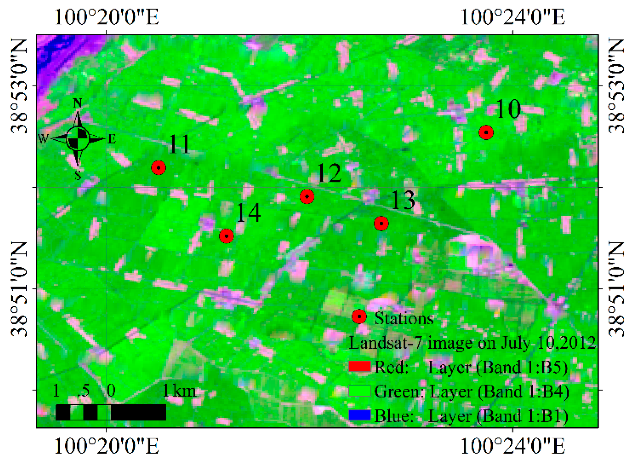
In this study, the observations by the EC systems and weather stations at five sites in the corn field were obtained from the “Heihe Plan Science Data Center, National Natural Science Foundation of China” (http://www.heihedata.org). These five sites are No. 10 to No. 14. Figure 2 shows the geographical location of the observation sites over oasis surfaces with a false-color Landsat-7 image of 10 July 2012 to show the underlying background. Several meteorological parameters were measured by the observation sites listed in Figure 2 from June to September in 2012. Six parameters among them are eligible for our study including near surface air temperature (°C), air relative humidity RH (%), solar down welling shortwave radiation (W/m2), friction velocity (m/s), sensible heat flux H (W/m2), and latent heat flux LE (W/m2). The H and LE measured using the EC system have been corrected for closure using the Bowen ratio closure method. More information about the HiWATER and MUSOEXE can be found in [28,29].
Additionally, four Moderate Resolution Imaging Spectroradiometer (MODIS) products covering the same period from June to September in 2012 were collected in this study. They are Land Surface Temperature/Emissivity Daily L3 Global 1km products (MOD11A1 and MYD11A1) and Vegetation Indices 16-Day L3 Global 1km product (MOD13A2 and MYD13A2). The criterions “Pixel produced”, “good data quality”, “average emissivity error ≤ 0.02”, and “average LST error ≤ 2 K” were used to control LST data. Additionally, the vegetation index (VI) usefulness parameter in the MOD13A2 and MYD13A2 products Quality Assessment Science Data Sets was used to ensure the data quality of normalized difference vegetation index (NDVI). The NDVI data with a VI usefulness from 0000 (highest quality) to 1100 (lowest quality) were retained in this study, while the others were excluded. Daily NDVI during a 16-day interval were assumed to be invariant as done in [12,30].
The LST and NDVI were extracted directly from the pixel in which the observation station was located, because the land cover type in the study area is approximately homogeneous. Then, we matched the MODIS data with the in-situ observations by comparing the view time. The matched values were then utilized to compare the three theoretical methods for estimating the dry and wet edges. In the comparison, and were set as 0.95 and 0.98; and were set as 0.18 and 0.24; and the vegetation height () was set as 1.0 m according to the field observations over the study area [31]. To calculate and from and , maximum possible LAI is required [21]. Since the vegetation under each site is maize, a maximum possible LAI of 5.0 was selected in the Moran method [32]. FVC was calculated from NDVI using a non-linear relationship, i.e., FVC = [(NDVI − NDVImin)/(NDVImax − NDVImin)]2 where NDVImin and NDVImax were set as 0.2 and 0.86 [19].
4. Results
4.1. Determination of Dry and Wet Edges
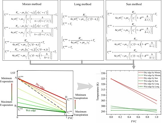
Figure 3 presents the estimation of , , , and by the three theoretical methods on sites from No. 10 to No. 12. The estimations on the other sites are not presented in this study since they have similar features as Figure 3. At each site, median values of , , , and during the study period were extracted. Based on these median values, we illustrated the estimated dry and wet edges at each site as shown in Figure 4. Corresponding to Figure 4, Table 1 was acquired by setting the maximum and minimum canopy resistance in the Moran method as infinity and zero, respectively. All of the results in Figure 3, Figure 4, and Table 1 indicate that:
(1) Dry edge
For the estimation of dry edge, the Sun method and the Long method are equal. They both suppose LE is equal to zero for dry bare soil and dry full-cover vegetation. The Moran method also supposes LE is equal to zero for dry bare soil. However, it does not hold this supposition for dry full-cover vegetation. The original Moran method suggests an empirical value of maximum stomatal resistance as 1000 ~ 1500 s/m for dry full-cover vegetation. We used the value of 1500 s/m in the calculation of Figure 3. It can be found that by Moran is generally lower than that by Long and Sun. Resultantly, the dry edge in the LST/FVC space estimated by Moran is lower than that of the other two methods as shown in Figure 4. However, it is notable that if the maximum canopy resistance for dry vegetation in the Moran method was set as infinity, the by Moran would be equal to that by Long and Sun as shown in Table 1.
(2) Wet edge
There are greater differences among the three theoretical methods for estimating wet edge as compared with estimating dry edge. The wet edge determined by the Long method is a horizontal line where and are both equal to the air temperature . The wet edge estimated by the Sun method is an oblique line and it is generally greater than that estimated by the Long method, as shown in Figure 3. In other words, and by the Sun method are both greater than that by the Long method. In contrast, by the Moran method is generally less than air temperature, which means that the sensible heat flux for saturated full-cover vegetation could be negative. Moreover, the by the Moran method is generally greater than that estimated by the other two methods. Resultantly, the wet edge by the Moran method is also an oblique line and crosses the wet edges by the Sun and Long methods as shown in Figure 4 and Table 1.
4.2. Estimation of LE
Furthermore, we compared the three theoretical methods for estimating LE by determining the dry and wet edges in a Two-source Model for estimating Evaporative Fraction (TMEF) [19]. The LE was estimated based on the same TMEF model and the same input parameters but with different boundaries of the LST/FVC space. For convenience, the maximum and minimum canopy resistance for dry vegetation in the Moran method were set as infinity and zero.
Figure 5 shows the scatter plots between estimated and observed LE. The scatter plots indicate that estimated LE by the Sun method and that by the Long method are comparable, and they have greater differences with the estimated LE by the Moran method. The estimations of LE by the Sun and Long methods show better agreement with the in-situ observations of LE. Two specific evaluation indicators, determination coefficient (R2) and Root-Mean-Square-Error (RMSE), are also presented in Figure 5. The R2 values by the Sun and Long method are greater than those by the Moran method, and the RMSE values by the Sun and Long method are less than those by the Moran method. R2 and RMSE values by the Sun and Long methods are very close. Taking the station of No. 11, for example, the R2 and RMSE are 0.66 and 69.85 for the Sun method, respectively, 0.68 and 68.50 for the Long method, respectively, and 0.57 and 78.86 for the Moran method, respectively. The same trend can be found at the sites of No. 10, No. 12, No. 13, and No. 14. The R2 and RMSE values at No. 14 are 0.57 and 75.69 for the Sun method, respectively, 0.59 and 75.83 for the Long method, respectively, and 0.46 and 88.13 for the Moran method, respectively. In summary, the Long and Sun methods are comparable with each other in this study. They are more appropriate than the Moran method in determining the dry and wet edges for estimating LE.
5. Discussion
5.1. Differences and Relations
The three theoretical calculation methods are all derived from the land surface energy balance equation. Although they were presented in different forms, we found they have similar mathematical expressions by revisiting their method physics. The prime difference among them is the determination of LE. The Moran method requires canopy resistance to determine LE. It infers the dry and wet edges through the adjustment of canopy resistance. For the bare soil components, canopy resistances on the dry and wet edges are equal to infinity and zero values. For the vegetation components, canopy resistances on the dry and wet edges are approximated to some empirical values. The Long method directly assumes LE equaling to zero on the dry edge and assumes LE equaling to available energy (i.e., H equaling to zero) on the wet edge. The Sun method introduces the Priestley-Taylor method to determine LE and calculates the dry and wet edges by adjusting the Priestley-Taylor parameter. On the dry and wet edges, the Priestley-Taylor parameter is respectively set as zero and an empirical maximum.
The differences in calculating LE led to different boundaries of the LST/FVC space. For determining the dry edge, the three theoretical methods are almost the same. That is because LE on the dry edge is considered to approximate zero for all the three methods, especially when the canopy resistance of vegetation and the Priestley–Taylor parameter on the dry edge are, respectively, set as infinity and zero. With respect to the wet edge, the three theoretical methods show greater difference. Generally, Long’s wet edge is a horizontal line equaling to . Sun’s wet edge is an oblique line and higher than Long’s wet edge. Moran’s wet edge intersects Long’s and Sun’s wet edges with a higher and a lower .
5.2. Suggestions
Among the three methods, the Sun method and the Long method are suggested in this study. Firstly, Table 2 shows some general and special parameters of the three theoretical methods. This table and the calculation equations of the three methods indicate that the Moran method is the most complex one and requires the most input parameters. Particularly, it requires some parameters that are hard to obtain, such as water vapor deficit and canopy resistance. The Sun and Long methods are much simpler than the Moran method. Moreover, they circumvent some complex and barely accessible parameters (i.e., , , ). Secondly, we compared the three theoretical methods for estimating LE using the same TMEF model and the same input parameters. Results demonstrated that the Sun and Long methods outperform the Moran method. Thirdly, on the Moran’s wet edge is generally less than (see Figure 3), which implies that the sensible heat flux of vegetation components with saturated water supply is generally negative and its latent heat flux is greater than the available energy.
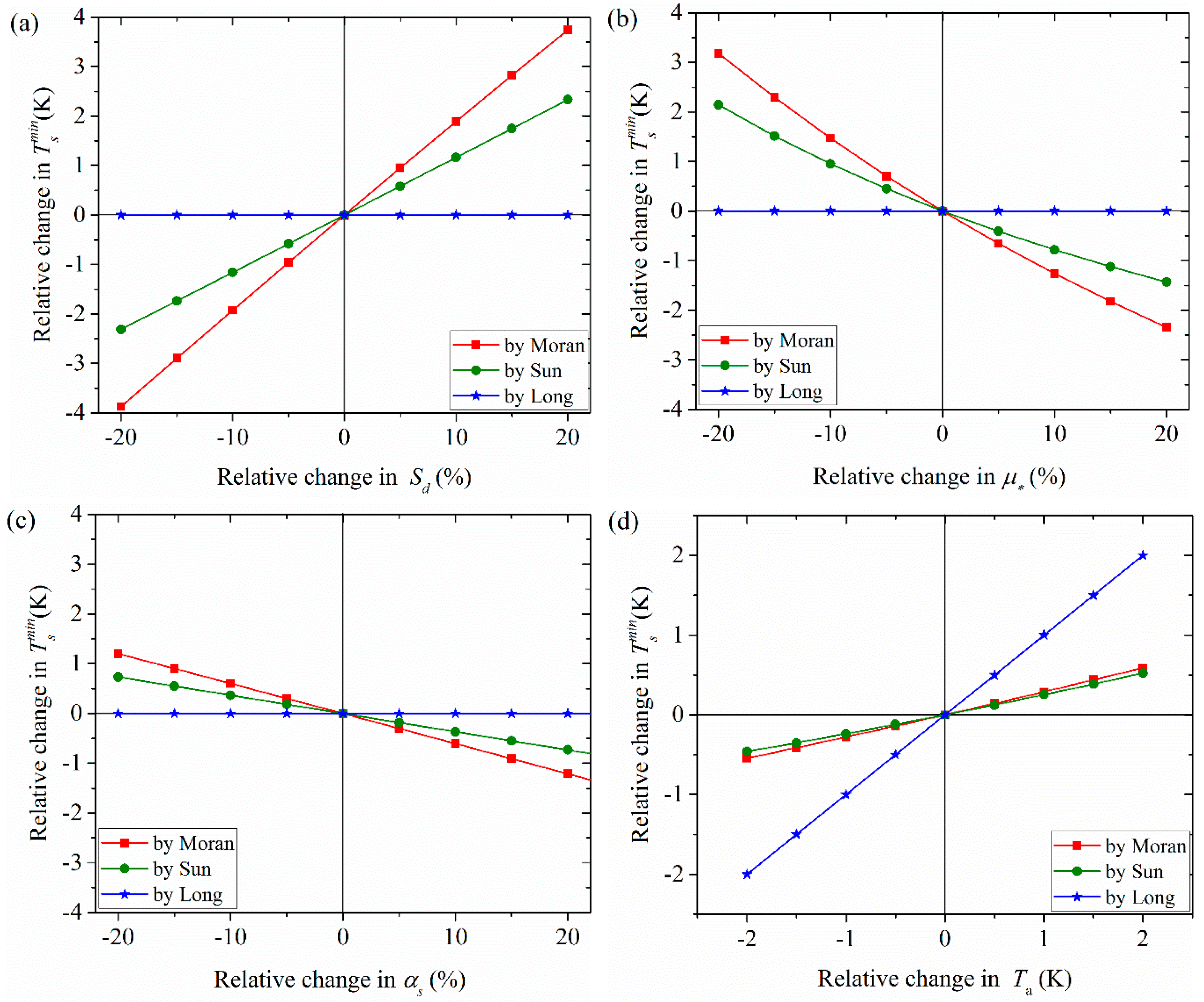
Further, a sensitivity analysis was performed in this study. We compared the relative change of a new estimated or to its initial value with the relative change of a new input variable to its initial value. The selected parameters are , , , , and with initial values of 798.80 (W/m2), 0.25 (m/s), 0.24, 0.18, and 285.82 (K), respectively. Results are presented in Figure 6 and Figure 7. It can be found that a slight perturbation in the input parameters would bring greater error in the Moran method than in the Sun and Long methods except for . A 20% perturbation in causes more than a 1 K error in the estimation of and almost a 4 K error in estimating by the Moran method. In contrast, a 20% perturbation in causes less than a 1 K error in and less than a 3 K error in by the Sun method. The same phenomena can be found for the perturbations in , , and . As for the perturbation in , approximate sensitivity was found between the Moran and Sun methods. This sensitivity analysis provides another argument for our suggestion.
As for the Sun and Long methods, we prefer the former one although the latter one is simpler. This is because the and are only correlated with in the latter one. Figure 6 and Figure 7 demonstrated that there are not any variations in the and estimated by the Long method when , , , and change from −20% to 20%. Additionally, determining the wet edge temperature as in the Long method implies that the EF on the wet edge is a constant value of 1, but EF is controlled not only by but also by wind speed [23]. Yang et al. (2015) indicated that the underestimation of temperatures for the wet edge is a main reason for underestimating EF in the hybrid dual-source scheme and trapezoid framework–based evapotranspiration model (HTEM) model [13]. The wet edge by the Sun method is higher than that by the Long method. Therefore, the Sun method is preferred to determine the dry and wet edges of the LST/FVC space.
6. Conclusions
In this study, we revisited and compared three theoretical methods for determining the dry and wet edges of LST/FVC space, i.e., Moran, Long, and Sun methods. Results are concluded here:
(a) For determining the dry edge, the Sun method is equal to the Long method. They are a little bit different from the Moran method. However, if the canopy resistance of dry full-covered vegetation is set as infinity, all of the three method are identical. At that time, LE on the dry edge is equal to zero.
(b) For determining the wet edge, the three methods have greater differences. Long’s wet edge is a horizontal line equaling air temperature. Sun’s wet edge is an oblique line and is higher than that of Long’s. Moran’s wet edge intersects with the wet edges of Long and Sun methods with a higher soil component temperature and a lower vegetation component temperature.
(c) Among the three methods, the Sun and Long methods are suggested for estimating LE or monitoring variation of soil moisture, because they are simpler in calculation; they can circumvent some complex parameters; and they had better performance in estimating LE. We are more inclined to the Sun method since Long’s wet edge is only correlated with air temperature.
From the Moran method to the Sun and Long methods, complex and barely accessible parameters decrease and performance in estimating LE is not necessarily lost. This implies that it is possible to determine the dry and wet edges using easily accessible parameters or parameters obtained from the image itself in the future. For example, air temperature is an essential parameter in the Sun and Long methods. There are already some methods for estimating the air temperature using satellite images [14,30,33]. Consequently, in future work, it will be worthwhile to improve further the Sun and Long methods, making them only rely on easily accessible parameters.
Acknowledgments
This study is supported by the National Natural Science Fund of China (41501457). The author would like to thank Cold and Arid Regions Science Data Center at Lanzhou, China and Heihe Plan Science Data Center, National Natural Science Foundation of China for providing meteorological and eddy covariance system observations. Thanks are also expressed to NASA Land Processes Distributed Active Archive Center for providing the MODIS data.
Author Contributions
Hao Sun conceived and designed the experiments, performed the experiments, and wrote the paper; Hao Sun, Yanmei Wang, and Weihan Liu analyzed the data; Shuyun Yuan and Ruwei Nie contributed materials and analysis tool.
Conflicts of Interest
The authors declare no conflict of interest.
References
- Yang, J.; Gong, P.; Fu, R.; Zhang, M.; Chen, J.; Liang, S.; Xu, B.; Shi, J.; Dickinson, R. The role of satellite remote sensing in climate change studies. Nat. Clim. Chang. 2013, 3, 875–883. [Google Scholar] [CrossRef]
- Anderson, M.C.; Norman, J.M.; Diak, G.R.; Kustas, W.P.; Mecikalski, J.R. A two-source time-integrated model for estimating surface fluxes using thermal infrared remote sensing. Remote Sens. Environ. 1997, 60, 195–216. [Google Scholar] [CrossRef]
- Bastiaanssen, W.G.M.; Menenti, M.; Feddes, R.A.; Holtslag, A.A.M. A remote sensing surface energy balance algorithm for land (sebal). 1. Formulation. J. Hydrol. 1998, 212–213, 198–212. [Google Scholar] [CrossRef]
- Allen, R.G.; Tasumi, M.; Trezza, R. Satellite-based energy balance for mapping evapotranspiration with internalized calibration (metric)—Model. J. Irrig. Drainage Eng.-ASCE 2007, 133, 380–394. [Google Scholar] [CrossRef]
- Cai, G.; Xue, Y.; Hu, Y.; Wang, Y.; Guo, J.; Luo, Y.; Wu, C.; Zhong, S.; Qi, S. Soil moisture retrieval from modis data in northern China plain using thermal inertia model. Int. J. Remote Sens. 2007, 28, 3567–3581. [Google Scholar] [CrossRef]
- Li, Z.L.; Tang, R.L.; Wan, Z.M.; Bi, Y.Y.; Zhou, C.H.; Tang, B.H.; Yan, G.J.; Zhang, X.Y. A review of current methodologies for regional evapotranspiration estimation from remotely sensed data. Sensors 2009, 9, 3801–3853. [Google Scholar] [CrossRef] [PubMed]
- Wang, K.C.; Dickinson, R.E. A review of global terrestrial evapotranspiration: Observation, modeling, climatology, and climatic variability. Rev. Geophys. 2012, 50. [Google Scholar] [CrossRef]
- Petropoulos, G.P.; Ireland, G.; Barrett, B. Surface soil moisture retrievals from remote sensing: Current status, products & future trends. Phys. Chem. Earth Parts A/B/C 2015, 83–84, 36–56. [Google Scholar]
- Jiang, L.; Islam, S.; Guo, W.; Jutla, A.S.; Senarath, S.U.S.; Ramsay, B.H.; Eltahir, E.A.B. A satellite-based daily actual evapotranspiration estimation algorithm over south florida. Glob. Planet. Chang. 2009, 67, 62–77. [Google Scholar] [CrossRef]
- Tang, R.; Li, Z.-L.; Tang, B. An application of the ts-vi triangle method with enhanced edges determination for evapotranspiration estimation from modis data in arid and semi-arid regions: Implementation and validation. Remote Sens. Environ. 2010, 114, 540–551. [Google Scholar] [CrossRef]
- Carlson, T. An overview of the “triangle method” for estimating surface evapotranspiration and soil moisture from satellite imagery. Sensors 2007, 7, 1612–1629. [Google Scholar] [CrossRef]
- Sun, H. Two-stage trapezoid: A new interpretation of the land surface temperature and fractional vegetation coverage space. IEEE J. Sel. Top. Appl. Earth Obs. Remote Sens. 2016, 9, 336–346. [Google Scholar] [CrossRef]
- Petropoulos, G.; Carlson, T.; Wooster, M.; Islam, S. A review of TS/VI remote sensing based methods for the retrieval of land surface energy fluxes and soil surface moisture. Prog. Phys. Geogr. 2009, 33, 224–250. [Google Scholar] [CrossRef]
- Sun, H.; Chen, Y.; Gong, A.; Zhao, X.; Zhan, W.; Wang, M. Estimating mean air temperature using modis day and night land surface temperatures. Theor. Appl. Climatol. 2014, 118, 81–92. [Google Scholar] [CrossRef]
- Sandholt, I.; Rasmussen, K.; Andersen, J. A simple interpretation of the surface temperature/vegetation index space for assessment of surface moisture status. Remote Sens. Environ. 2002, 79, 213–224. [Google Scholar] [CrossRef]
- Wang, P.X.; Li, X.W.; Gong, J.Y.; Song, C.H. Vegetation temperature condition index and its application for drought monitoring. In Proceedings of the IEEE 2001 International Geoscience and Remote Sensing Symposium, 2001, (IGARSS ’01), Sydney, Australia, 9–13 July 2001; Volume 1, pp. 141–143. [Google Scholar]
- Long, D.; Singh, V.P. A modified surface energy balance algorithm for land (m-sebal) based on a trapezoidal framework. Water Resour. Res. 2012, 48, W02528. [Google Scholar] [CrossRef]
- Long, D.; Singh, V.P. A two-source trapezoid model for evapotranspiration (TTME) from satellite imagery. Remote Sens. Environ. 2012, 121, 370–388. [Google Scholar] [CrossRef]
- Sun, H. A two-source model for estimating evaporative fraction (TMEF) coupling priestley-taylor formula and two-stage trapezoid. Remote Sens. 2016, 8, 248. [Google Scholar] [CrossRef]
- Long, D.; Singh, V.P.; Scanlon, B.R. Deriving theoretical boundaries to address scale dependencies of triangle models for evapotranspiration estimation. J. Geophys. Res. Atmos. 2012, 117, 1–17. [Google Scholar] [CrossRef]
- Moran, M.; Clarke, T.; Inoue, Y.; Vidal, A. Estimating crop water deficit using the relation between surface-air temperature and spectral vegetation index. Remote Sens. Environ. 1994, 49, 246–263. [Google Scholar] [CrossRef]
- Peng, J.; Liu, Y.; Zhao, X.; Loew, A. Estimation of evapotranspiration from modis toa radiances in the poyang lake basin, China. Hydrol. Earth Syst. Sci. 2013, 17, 1431–2013. [Google Scholar] [CrossRef]
- Wang, K.C.; Li, Z.Q.; Cribb, M. Estimation of evaporative fraction from a combination of day and night land surface temperatures and NDVI: A new method to determine the priestley-taylor parameter. Remote Sens. Environ. 2006, 102, 293–305. [Google Scholar] [CrossRef]
- Jiang, L.; Islam, S. Estimation of surface evaporation map over southern great plains using remote sensing data. Water Resour. Res. 2001, 37, 329–3340. [Google Scholar] [CrossRef]
- Jiang, L.; Islam, S. A methodology for estimation of surface evapotranspiration over large areas using remote sensing observations. Geophys. Res. Lett. 1999, 26, 2773–2776. [Google Scholar] [CrossRef]
- Eichinger, W.E.; Parlange, M.B.; Stricker, H. On the concept of equilibrium evaporation and the value of the priestley-taylor coefficient. Water Resour. Res. 1996, 32, 161–164. [Google Scholar] [CrossRef]
- Lhomme, J.-P. A theoretical basis for the priestley-taylor coefficient. Bound. Layer Meteorol. 1997, 82, 179–191. [Google Scholar] [CrossRef]
- Li, X.; Li, X.W.; Li, Z.Y.; Ma, M.G.; Wang, J.; Xiao, Q.; Liu, Q.; Che, T.; Chen, E.X.; Yan, G.J.; et al. Watershed allied telemetry experimental research. J. Geophys. Res. Atmos. 2009, 114. [Google Scholar] [CrossRef]
- Liu, S.M.; Xu, Z.W.; Wang, W.Z.; Jia, Z.Z.; Zhu, M.J.; Bai, J.; Wang, J.M. A comparison of eddy-covariance and large aperture scintillometer measurements with respect to the energy balance closure problem. Hydrol. Earth Syst. Sci. 2011, 15, 1291–1306. [Google Scholar] [CrossRef]
- Sun, H.; Chen, Y.; Zhan, W. Comparing surface and canopy layer urban heat islands over Beijing using modis data. Int. J. Remote Sens. 2015, 36, 5448–5465. [Google Scholar] [CrossRef]
- Sun, J.; Hu, Z.-Y.; Xun, X.-Y.; Peng, W.; Lü, B.; Xu, L.-J. Albedo characteristics in different underlying surfaces in mid and upper-reaches of heihe and its impact factor analysis. Plateau Meteorol. 2011, 30, 607–613. (In Chinese) [Google Scholar]
- Yin, G.; Li, J.; Liu, Q.; Fan, W.; Xu, B.; Zeng, Y.; Zhao, J. Regional leaf area index retrieval based on remote sensing: The role of radiative transfer model selection. Remote Sens. 2015, 7, 4604. [Google Scholar] [CrossRef]
- Chen, Y.; Sun, H.; Li, J. Estimating daily maximum air temperature with modis data and a daytime temperature variation model in Beijing urban area. Remote Sens. Lett. 2016, 7, 865–874. [Google Scholar] [CrossRef]
Figure 1.
Diagram of the dry and wet edges in Land surface temperature and fractional vegetation coverage (LST/FVC) space [19].
Figure 1.
Diagram of the dry and wet edges in Land surface temperature and fractional vegetation coverage (LST/FVC) space [19].
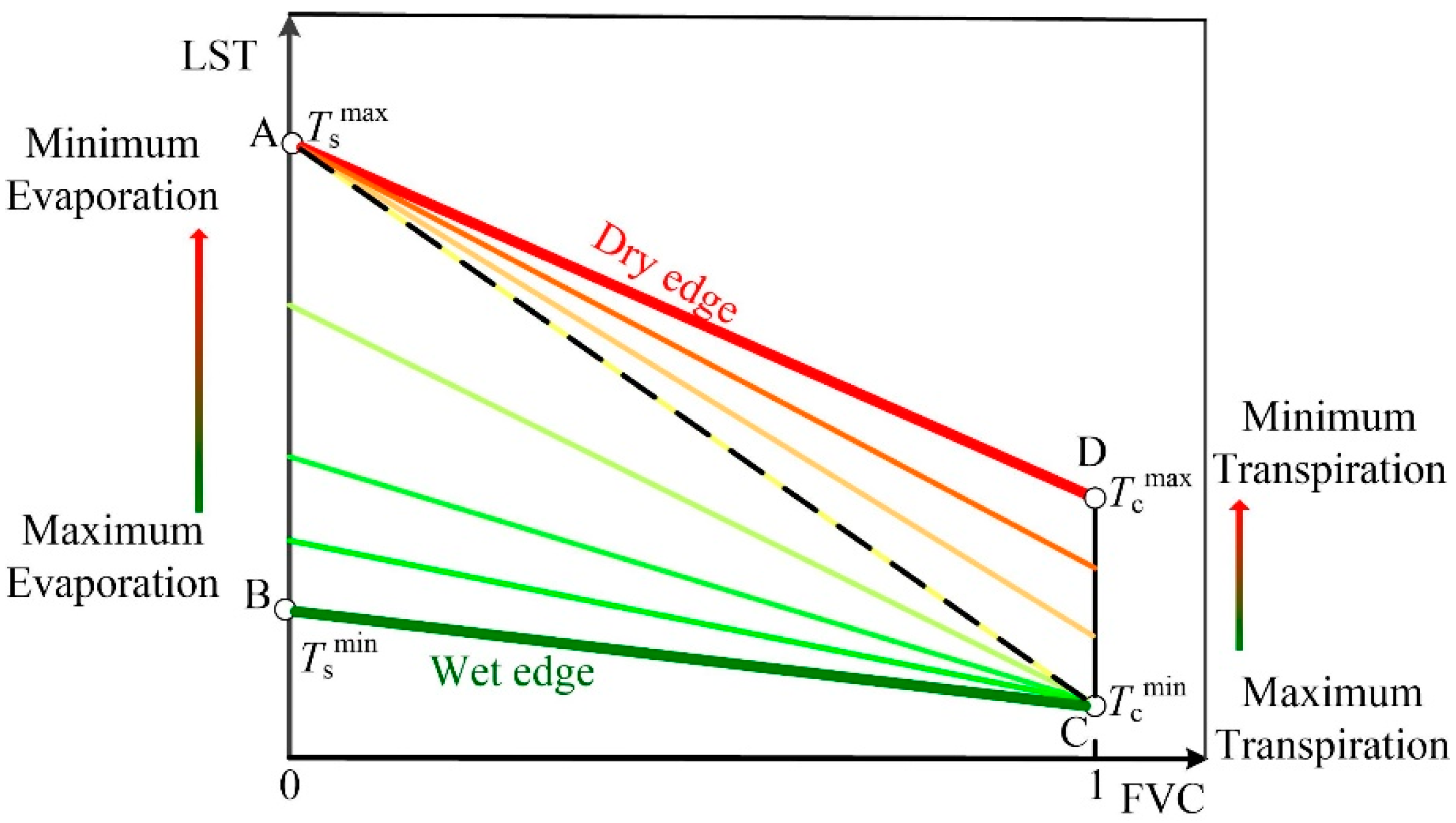
Figure 2.
Geographic location of the stations.

Figure 3.
LST components on dry and wet edges estimated by the three theoretical methods on different sites. (a,b) are on No. 10 site; (c,d) are on No. 11 site; (e,f) are on No. 12 site.
Figure 3.
LST components on dry and wet edges estimated by the three theoretical methods on different sites. (a,b) are on No. 10 site; (c,d) are on No. 11 site; (e,f) are on No. 12 site.
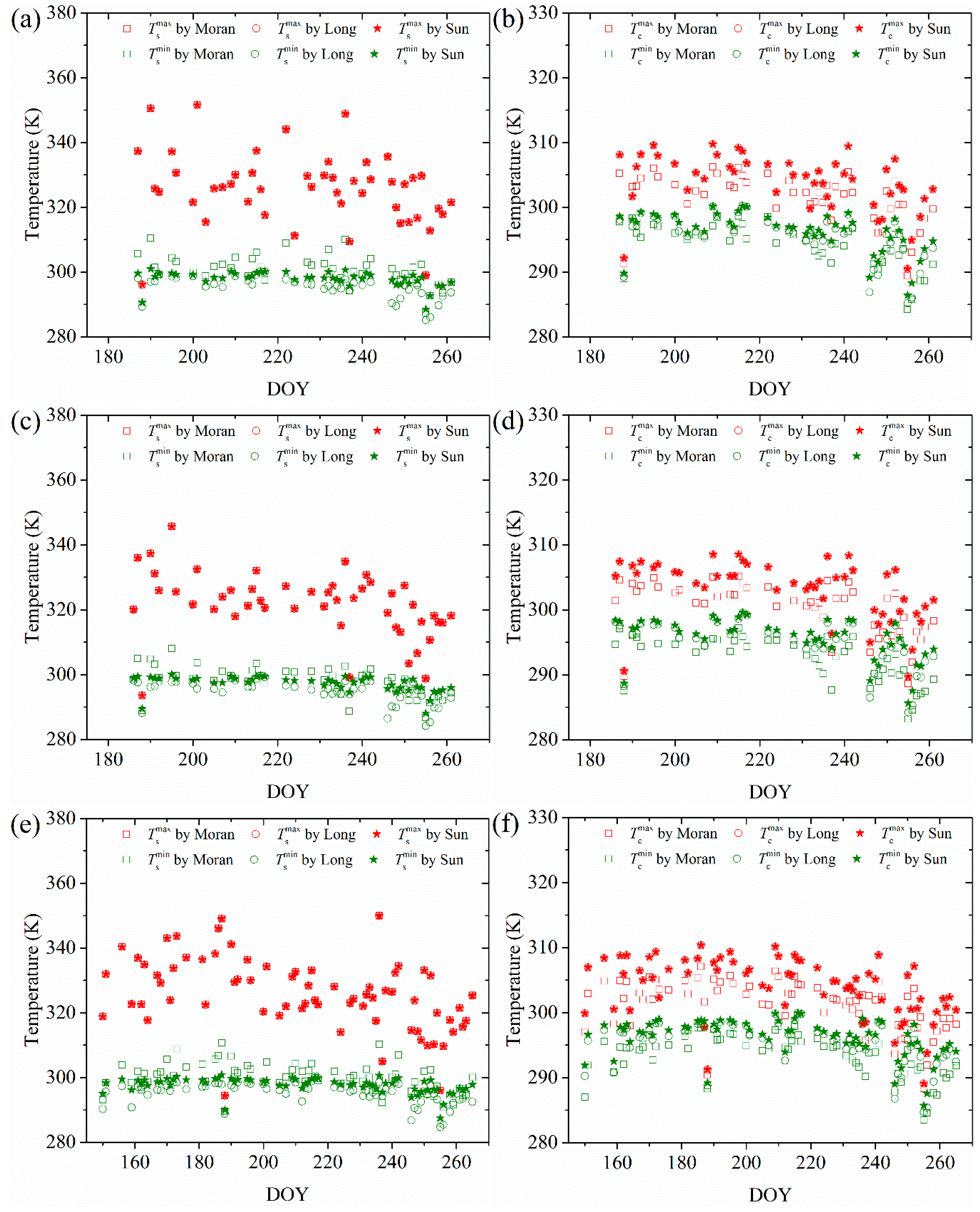
Figure 4.
Dry and wet edges estimated by the three theoretical methods on sites of (a) No. 10, (b) No. 11, (c) No. 12, and (d) No. 13 where the maximum and minimum canopy resistance were calculated using empirical parameters.
Figure 4.
Dry and wet edges estimated by the three theoretical methods on sites of (a) No. 10, (b) No. 11, (c) No. 12, and (d) No. 13 where the maximum and minimum canopy resistance were calculated using empirical parameters.
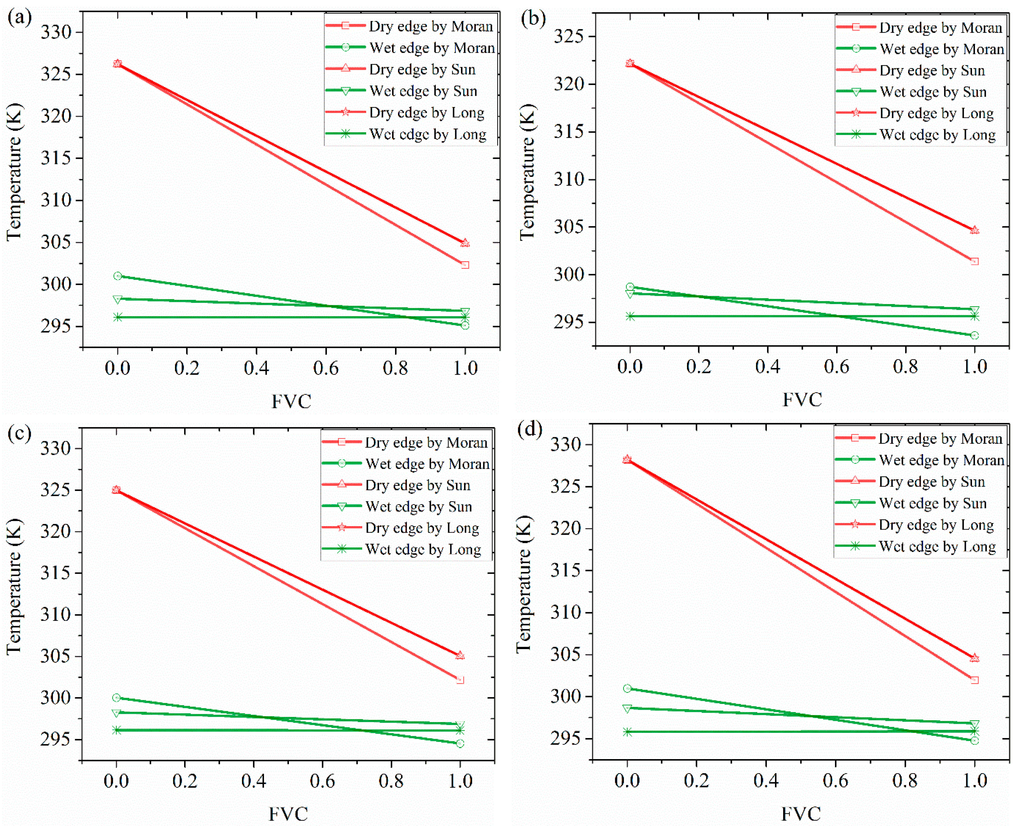
Figure 5.
Scatter diagram between estimated and observed LE at the site of (a) No. 10, (b) No. 11, (c) No. 12, and (d) No. 13.
Figure 5.
Scatter diagram between estimated and observed LE at the site of (a) No. 10, (b) No. 11, (c) No. 12, and (d) No. 13.
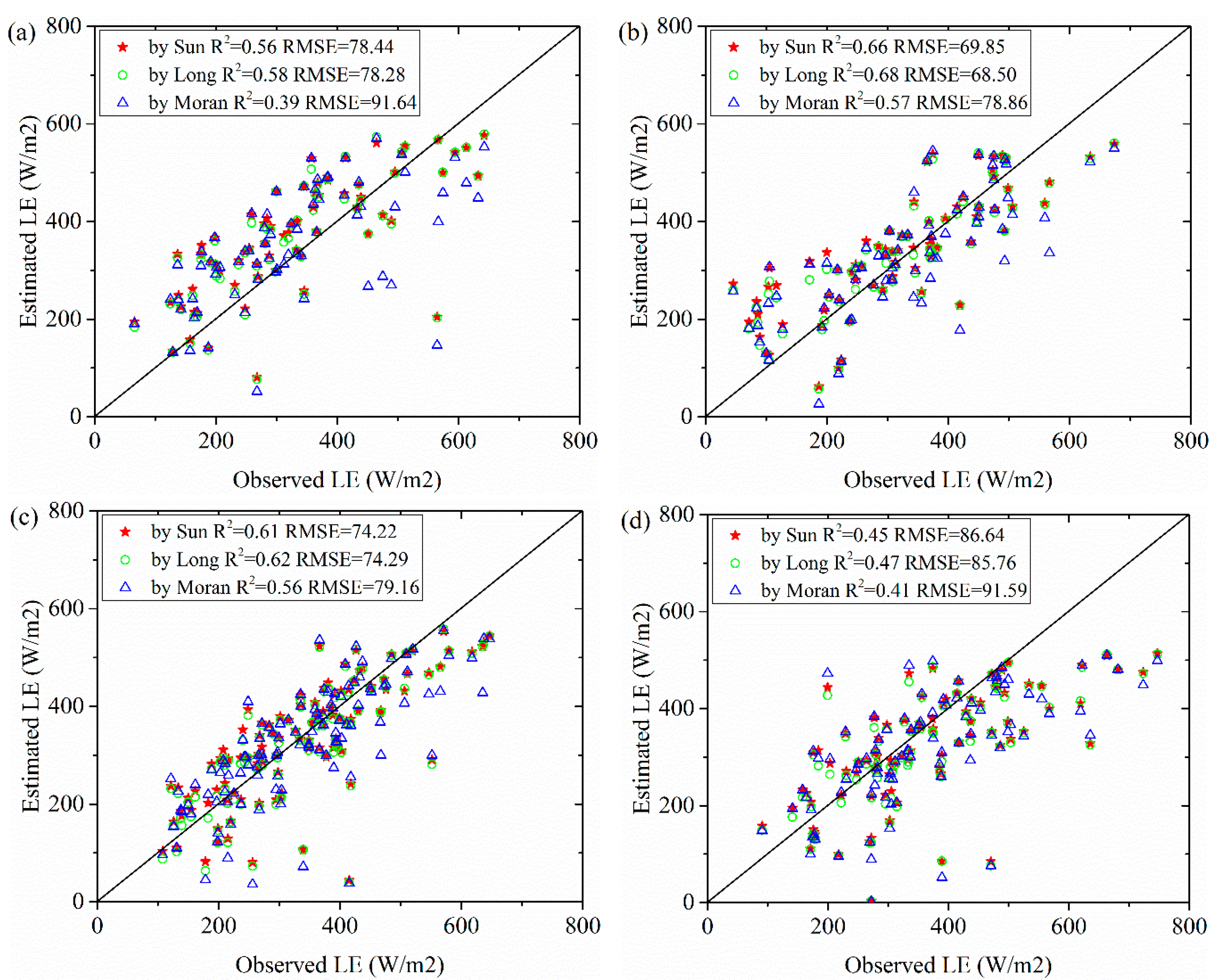
Figure 6.
Sensitivity analysis of the by the three theoretical methods to input parameters (a) , (b) , (c) , and (d) .
Figure 6.
Sensitivity analysis of the by the three theoretical methods to input parameters (a) , (b) , (c) , and (d) .
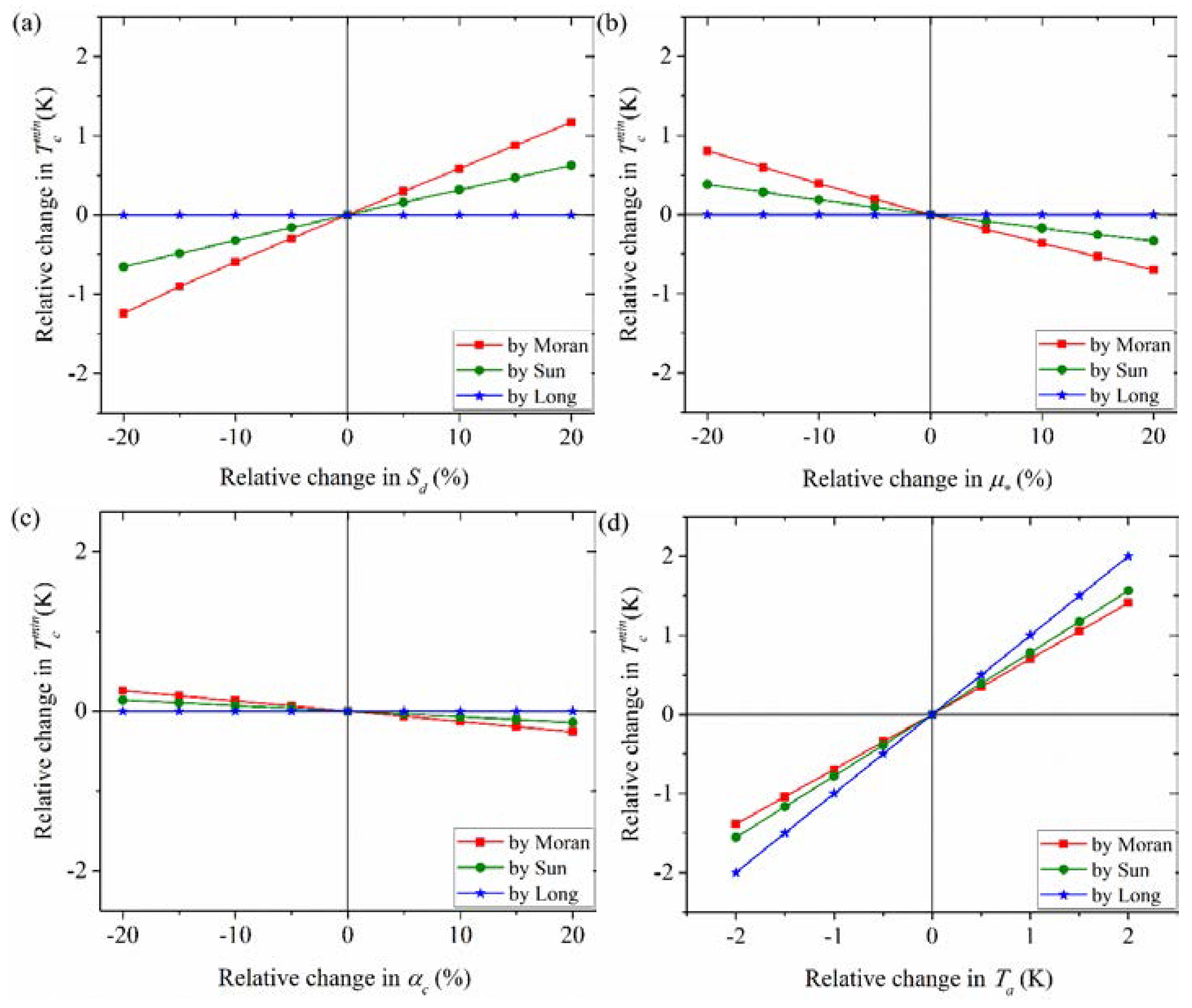
Figure 7.
Sensitivity analysis of the by the three theoretical methods to input parameters (a) , (b) , (c) , and (d)
Figure 7.
Sensitivity analysis of the by the three theoretical methods to input parameters (a) , (b) , (c) , and (d)

Table 1.
Dry and wet edges estimated by the three theoretical methods on sites of No. 10~No. 14 where the maximum and minimum canopy resistance were set as infinity and zero. FVC = fractional vegetation coverage.
Table 1.
Dry and wet edges estimated by the three theoretical methods on sites of No. 10~No. 14 where the maximum and minimum canopy resistance were set as infinity and zero. FVC = fractional vegetation coverage.
| Site | FVC | Moran’s Result (K) | Sun’s Result (K) | Long’s Result (K) | |||
|---|---|---|---|---|---|---|---|
| Dry Edge | Wet Edge | Dry Edge | Wet Edge | Dry Edge | Wet Edge | ||
| 10 | 0 | 326.21 | 301.01 | 326.21 | 298.31 | 326.21 | 296.12 |
| 1 | 302.30 | 295.12 | 304.89 | 296.86 | 304.89 | 296.10 | |
| 11 | 0 | 322.18 | 298.73 | 322.18 | 298.05 | 322.18 | 295.64 |
| 1 | 301.38 | 293.62 | 304.63 | 296.37 | 304.63 | 295.63 | |
| 12 | 0 | 324.99 | 300.04 | 324.99 | 298.29 | 324.99 | 296.15 |
| 1 | 302.18 | 294.54 | 305.06 | 296.88 | 305.06 | 296.10 | |
| 13 | 0 | 328.21 | 300.99 | 328.21 | 298.67 | 328.21 | 295.81 |
| 1 | 301.97 | 294.77 | 304.56 | 296.82 | 304.56 | 295.89 | |
| 14 | 0 | 322.59 | 298.11 | 322.59 | 297.99 | 322.59 | 296.34 |
| 1 | 302.05 | 293.89 | 305.11 | 297.01 | 305.11 | 296.34 | |
Table 2.
Input parameters of the three theoretical methods.
| Methods | Special Parameters | General Parameters |
|---|---|---|
| Moran method | , , , , , , | , , , , , , , |
| Long method | , | |
| Sun method | , , , |
© 2017 by the authors. Licensee MDPI, Basel, Switzerland. This article is an open access article distributed under the terms and conditions of the Creative Commons Attribution (CC BY) license (http://creativecommons.org/licenses/by/4.0/).
Share and Cite
MDPI and ACS Style
Sun, H.; Wang, Y.; Liu, W.; Yuan, S.; Nie, R. Comparison of Three Theoretical Methods for Determining Dry and Wet Edges of the LST/FVC Space: Revisit of Method Physics. Remote Sens. 2017, 9, 528. https://doi.org/10.3390/rs9060528
AMA Style
Sun H, Wang Y, Liu W, Yuan S, Nie R. Comparison of Three Theoretical Methods for Determining Dry and Wet Edges of the LST/FVC Space: Revisit of Method Physics. Remote Sensing. 2017; 9(6):528. https://doi.org/10.3390/rs9060528
Chicago/Turabian StyleSun, Hao, Yanmei Wang, Weihan Liu, Shuyun Yuan, and Ruwei Nie. 2017. "Comparison of Three Theoretical Methods for Determining Dry and Wet Edges of the LST/FVC Space: Revisit of Method Physics" Remote Sensing 9, no. 6: 528. https://doi.org/10.3390/rs9060528
Note that from the first issue of 2016, this journal uses article numbers instead of page numbers. See further details here.