1. Introduction
The development of remote sensing systems based on ultraviolet (UV) cameras for gas detection in the atmosphere has been growing in recent years. Focus has been primarily on the quantification of volcanic sulphuric dioxide (SO
2) emissions, and more recently, on emissions from industrial sources. Since the pioneering work of Mori and Burton [
1] and Bluth et al. [
2], several studies (Burton et al. [
3]) and intercomparisons (Kern et al. [
4]) have been performed on volcanic emissions and fumarolic fields (Tamburello et al. [
5]). The use of UV cameras has the advantage of providing images with high spatial and temporal resolution, providing more information in a single reading than other techniques, such as scanning methods with similar outputs (two dimensional SO
2 map) like Imaging Differential Optical Absorption Spectroscopy (IDOAS) [
6]. Some issues concerning UV cameras have been discussed in the literature, for example, light dilution effects (Mori et al. [
7], Campion et al. [
8]), calibration issues (Lübcke et al. [
9]), image corrections (e.g., vignetting and others effects), and the selection of different system parameters (Kantzas et al. [
10], Kern et al. [
11]). Further, with a similar approach using images acquired at different wavelengths, water fluxes from volcanic plumes can be quantified (Pering et al. [
12]).
This technique was more recently employed for monitoring anthropogenic SO
2 emissions to the atmosphere from sources such as power plants, oil refineries or, more broadly, any industrial stack, provided these are strong enough to overcome the detection limit. A low-cost design (Wilkes et al. [
13]) of this kind of systems helps to reach that objective. Those emissions have been largely studied with scanning methods based on Differential Optical Absorption Spectroscopy (DOAS) (Platt and Stutz [
14]), including stationary ground based measurements with multi axis—DOAS (MAX-DOAS) (Rivera et al. [
15], Frins et al. [
16]), and mobile measurements (e.g., Rivera et al. [
17], Frins et al. [
18]). Consistent results are obtained between the emission rates found by the application of those methods and data obtained from in situ devices, validating these techniques.
In comparison with the large amount of work on volcanic plumes, few measurements of anthropogenic sources have been performed with UV cameras. Early studies were carried out by McElhoe and Conner [
19], Dalton et al. [
20]. More recently, Smekens et al. [
21] have remotely measured emissions from a coal-burning power plant using an UV SO
2 camera system, obtaining good agreement with data provided by sensors located within the stacks. Further, a SO
2 camera system to measure ship emissions was used by Prata [
22].
Some specific problems may arise when UV cameras are used to quantify emissions of anthropogenic sources. For example, typical industrial emissions have lower concentration of SO2 than volcanoes, so the detection limit plays an important role. Also, the acquisition of a SO2-free (clean) reference image for an accurate retrieval can sometimes be complicated, due to the landscape surrounding the stacks, both in industrial environments or volcanoes. To solve this, a great effort to obtain the background images is required, as discussed below. Furthermore, in systems consisting of two cameras, pixels with the same coordinates in both cameras do not necessarily correspond to the same spatial point. Thus, it is necessary to find a correlation between the two images, prior to applying any evaluation method.
A method to obtain background images is by pointing the UV cameras to an emission-free sky region, which is especially troublesome on cloud days. Some authors (see [
4,
10,
21]) have also presented methods to estimate the background behind the plume from two emission images. However, most of those works are restricted to deal with clear sky or almost homogeneously illuminated days. The method proposed by Smekens et al. [
21] deserves special attention. They apply a polynomial fit to the sky images that include the SO
2 plume. Then, a transmittance image is calculated by taking the ratio between the original image and the polynomial approximation. Finally, applying an iterative thresholding procedure, they intend to extract (segment) the plume region. On cloudy days, however, the sky image could present spurious structures, similar to the ones appearing in the plume image, so the described procedure does not always allow distinguishing between plume and clouds.
In the present paper, we describe a new (non-iterative) procedure to estimate the intensity background behind the plume, before light has traversed it. Thus, instead of four images (two images of the SO2-plume and two images of the background), only images of the plume are necessary. The first step of the proposed method involves the segmentation of the SO2-plume from the emission images, by taking the ratio between the (raw) sky images at two specific wavelengths, λon and λoff, where the SO2-absorption cross-section is significantly different (see below). This approach is efficient in locating the plume region still under cloudy conditions. The second step consists of a polynomial interpolation procedure to estimate the light intensity behind the plume.
The purpose of this work is to present our new two-image method (2-IM) that uses background images constructed from the emission images, and to compare its performance with the four-images method (4-IM), which uses as background sky images acquired at a different viewing direction relative to the emission images.
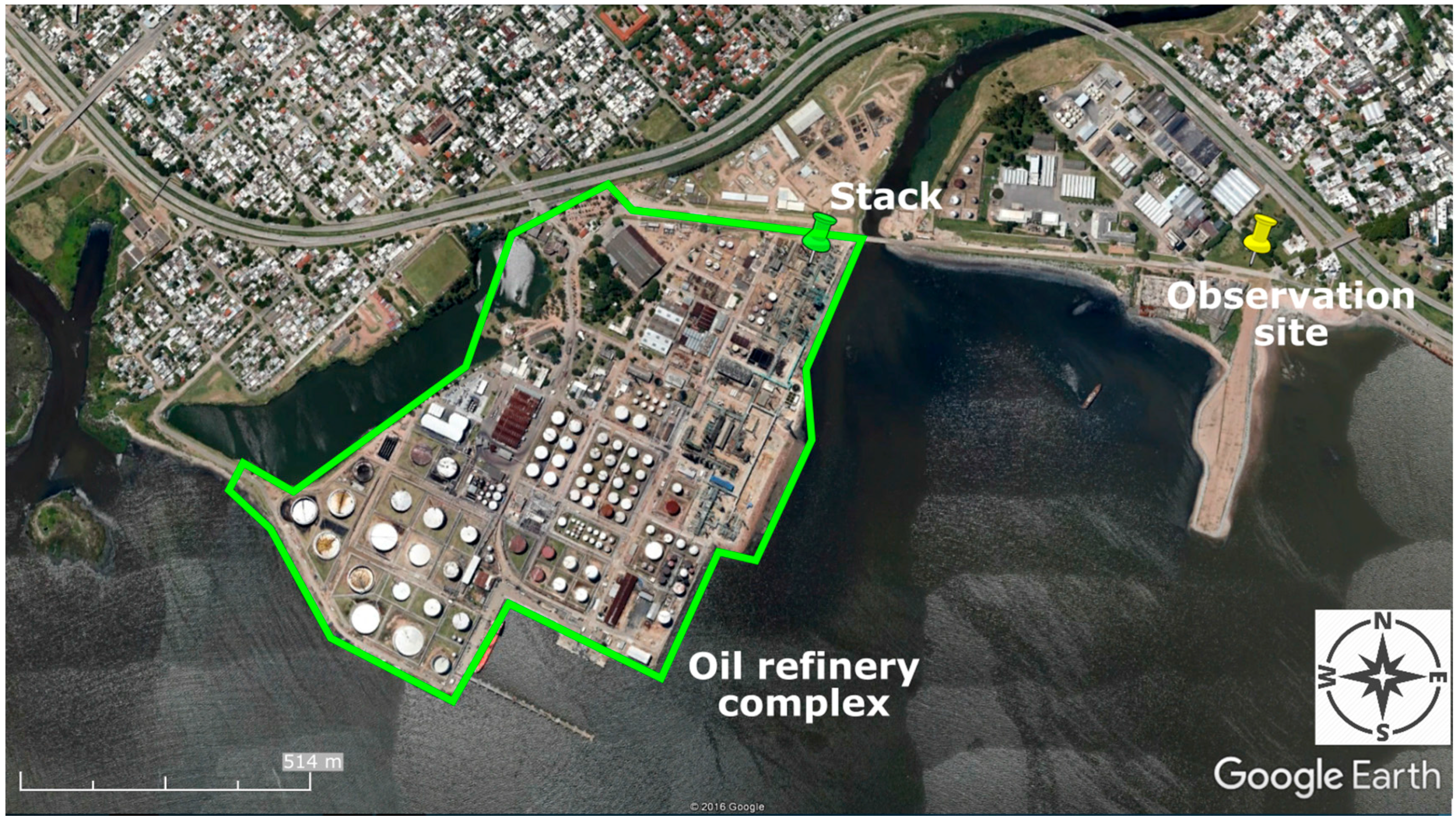
We tested the 4-IM and 2-IM approaches by performing measurements of SO2-emissions from a stack of an oil refinery placed in Montevideo City, Uruguay. The optical system used consists of two ultraviolet sensitive cameras provided with narrow band UV filters, which can simultaneously acquire two images at different wavelengths. Considerations on image processing and system detection limits are discussed. We also compared the results with MAX-DOAS measurements.
In the next section, the basics of the measurement techniques are presented. The experimental setup and results are discussed in
Section 3 and
Section 4, respectively. Conclusions are presented in
Section 5.
2. SO2-Emission Retrieval with UV-Cameras
2.1. Radiative Transfer Considerations
Based on the Lambert-Beer law, the light reaching a detector after passing through a certain air mass (e.g., a plume containing several trace gases and aerosols) can be expressed as:
where
λ is the wavelength,
I(
λ) and
I0(
λ) are the light intensities after and before traversing the air mass, respectively,
σk(
λ) is the absorption cross-section of the
k-th gas species present in the air mass,
ck(
l) its concentration, and
l denotes the optical path inside the air mass.
εs is the scattering extinction coefficient due to aerosols present in the air mass. Equation (1) is valid as long as the aerosol load is low enough to ensure single scattering processes.
When using UV cameras, I(λ) and I0(λ) are represented by images filtered by the instrument function of the optical system. These images will be denoted as I(λ,i,j) and I0(λ,i,j), respectively, where (i,j) are pixel coordinates. Roughly, we can say that I(λ,i,j) is an image (at wavelength λ) of the gas emission, while I0(λ,i,j) is an image of the background intensity before light traverses the plume.
In the following, we will assume that there is only one absorbing trace gas species, specifically SO
2, and we will consider two specific wavelengths:
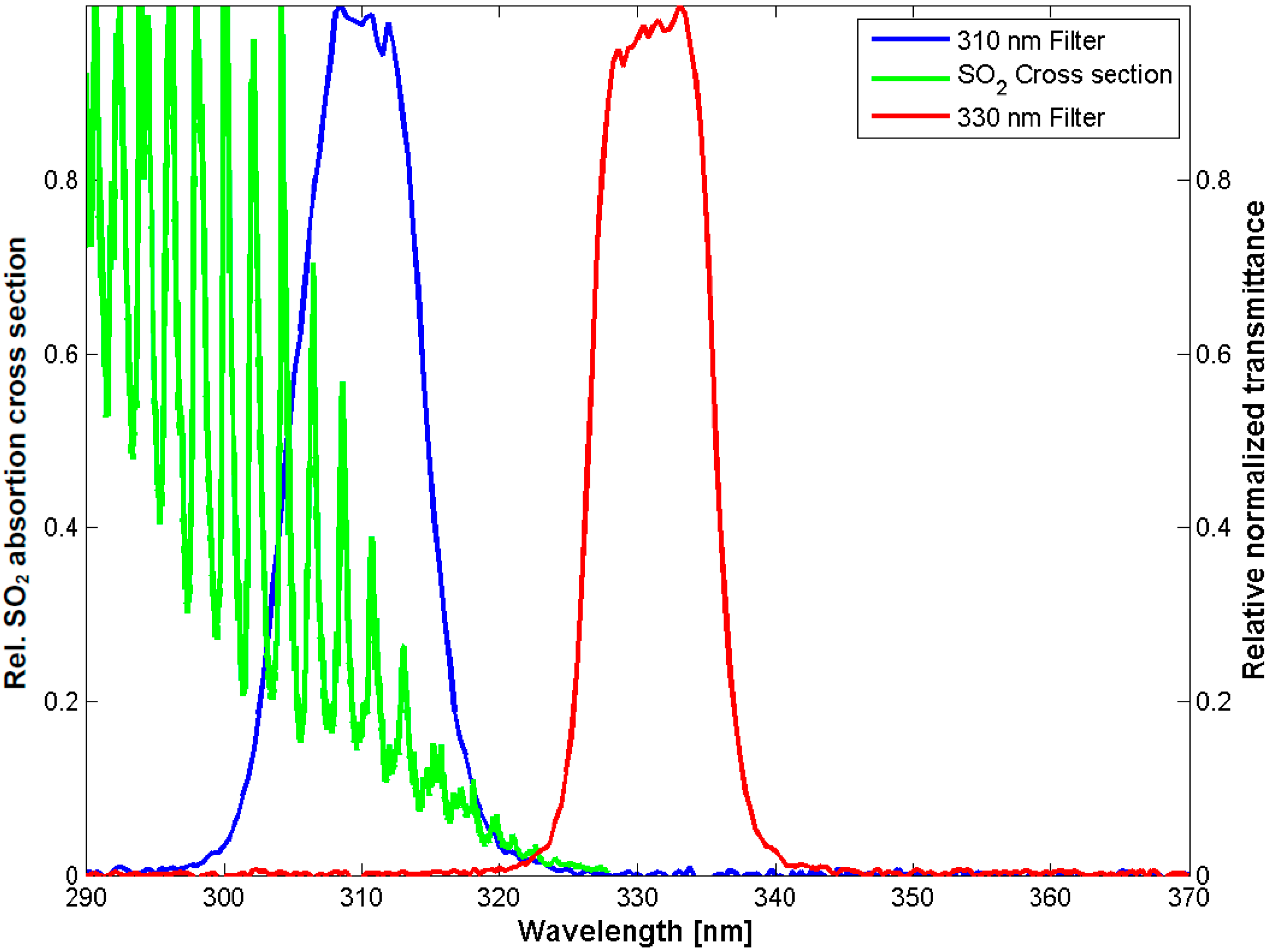
λon is chosen in the spectral range where the SO
2-absorption cross-section is high, and
λoff lies as close as possible to
λon, but the SO
2-absorption cross-section is almost negligible. In this work,
λon is ~310 nm and
λoff is ~330 nm (the full detail can be seen in
Section 3.2).
From (1), the optical depths at these wavelengths are:
and
To describe Mie scattering at
λon,off, it is assumed (see e.g., [
14],
Section 4.2):
where
α is the Angström exponent.
Then, from (2) and (4), the cumulative optical depth due to the SO
2 absorption along the optical path reaching the pixel (
i,j) will be:
Substituting (3) into (5), we obtain an expression for the SO
2 optical depth:
In the particular case when one assumes that in the volume of interest (e.g., a plume) no aerosols are present, one has
εs(
λoff,l) = 0, and then:
And thus, expression (6) reduces to:
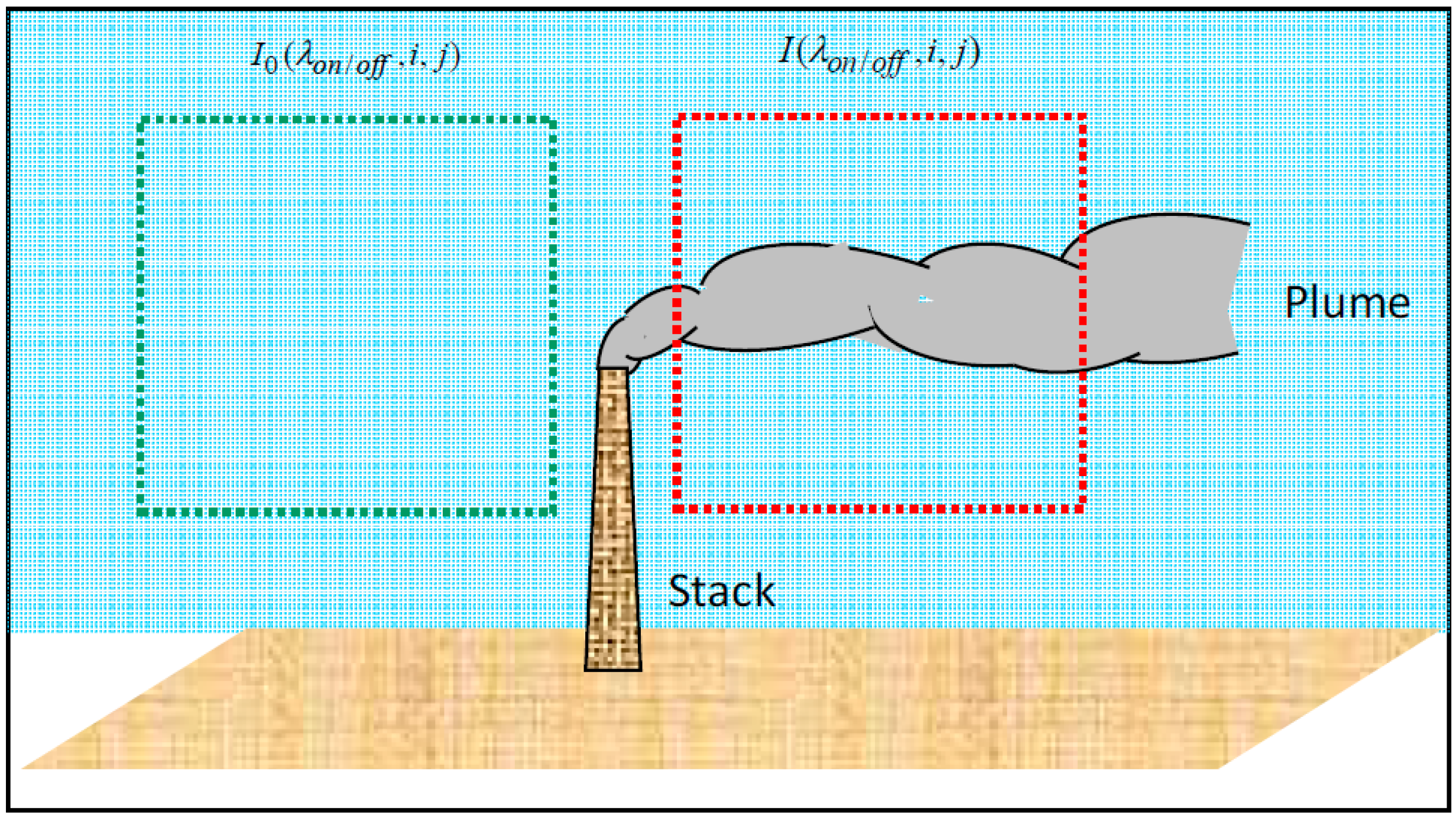
In general, however, four images are necessary for retrieving a 2D-map of the cumulative SO2 optical depth (τSO2), as shown in Equation (6). Two of them, I(λon/off,i,j), are images of the emission of a certain source, e.g., images of the plume of a SO2-emitting stack, and the other two, I0(λon/off,i,j), are images of the background.
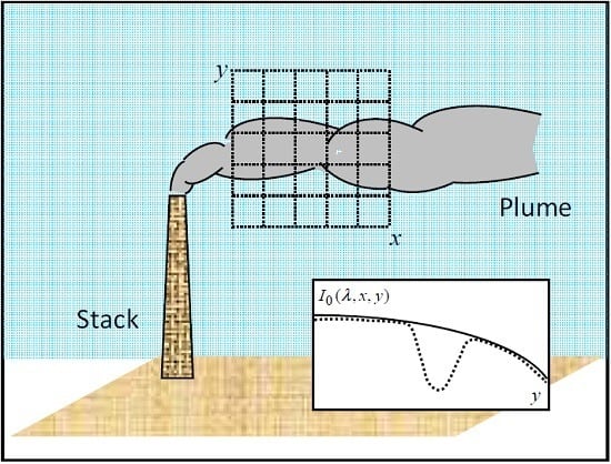
In the example of a plume emitted by a stack, the background images should be images of the light intensity behind the plume, which are impossible to acquire from a remote site in the presence of the plume. The typical way (see e.g., [
9,
11]) of acquiring background images is by changing the viewing direction to obtain plume-free images of the sky, as schematically illustrated in
Figure 1. In practice, this could mean a 90° change in looking direction.
Figure 1 depicts a broad panorama of the region to be considered. The region delimited by the dashed red lines allows obtaining the emission images, while the region delimited by the dashed green lines allows obtaining the emission-free background images. Henceforth, this imaging procedure will be called the four-image method (4-IM).
The procedure described above works well if the illumination in the background viewing direction is approximately equal to that in the plume direction, since the light reaching the cameras depends on the solar zenith and azimuth angle, assuming no clouds are present. Additional posterior corrections could be necessary, according to user criterion, for example, subtracting a constant offset from the image as proposed by Mori and Burton [
1].
In order to reduce the number of images needed to retrieve the SO2 map (τSO2) from Equation (6), in the following section we propose constructing plume-free background images (I0(λon/off,i,j)) through an interpolation from a portion of emission free sky available in the two emission images I(λon/off,i,j). Henceforth, this approach will be called the two-image method (2-IM).
2.2. 2-IM Approach: Artificial Background Generation
Since the optical system consists of two cameras for acquiring images at different wavelengths, pixels with the same coordinates in both cameras do not necessarily correspond to the same spatial point. Thus, prior to applying any evaluation method (2-IM or 4-IM), the process starts with an image pre-processing for establishing a correspondence between pixels of different cameras. This starts with the subtraction of the dark current images. After that, a binary segmentation is performed in order to keep the same shapes at both wavelengths, i.e., stacks. Then, a 2D cross correlation is made to obtain the correspondence between pixels in the images acquired by both cameras. All these steps are performed in an automatic way.
For the sake of simplicity, to build the artificial background images (
I0(
λon/off,i,j)), we will assume that the plume moves almost horizontally and the light intensity on each side of the plume (immediately above and below) is similar to that directly behind the plume, and that the plume cross section is small in comparison with the whole image. We will model the background as:
where (
x,y) is a Cartesian coordinate system (with
x and
y along the horizontal and vertical direction, respectively).
p is a low degree (e.g., third to fifth degree) polynomial matching the sky intensity on each side of the plume and filling the gap in the region inside it, as schematically illustrated in
Figure 2 (the procedure described above could be applied when the plume moves in any arbitrary direction.)
The procedure to build artificial background images through polynomial fitting requires processing the emission images
I(
λon/off,i,j). The first step is to know the position of the plume in the images. To do this, we compute the quotient
I(
λon,i,j)/
I(
λoff,i,j). The intensity quotient on the plume is smaller than in the surrounding sky, due to the SO
2 absorption at
λon. Thus, this operation does not alter the contrast between plume and background, and eliminates clouds structures because they are present in both wavelengths. After that, a global thresholding is performed, and the result is labelled by connecting neighbour pixels with 8-connectivity, i.e., a pixel
z with coordinates (
i,j) and its 8 adjacent neighbors that fulfil the condition to have the same image values as
z. These two conditions, location and value, determine if the pixel belongs to the “neighbors vicinity with 8-connectivity” or not, defining and labelling each simply connected region (Gonzalez and Woods [
23]). Thus, the plume is obtained by selecting the region with the larger number of labels.
Our automatic (and non-iterative) plume segmentation approach could be useful when large numbers of images have to be processed.
Once the plume is segmented from the images
I(
λon/off,i,j), we take vertical profiles at horizontal separations of one pixel. For every vertical profile without plume, a low-order polynomial fit (filling the gap) is applied, as illustrated in the inlet of
Figure 2. This generates a sheet that approximates the background at the position of the plume. A more detailed description of the procedure is given in
Section 4.
The dashed curve in the inlet of
Figure 2 depicts a vertical intensity cut across the plume, while the solid curve illustrates the polynomial fit needed to generate the artificial background images. The fitting procedure allows estimating the light intensity behind the plume.
4. Results and Discussion
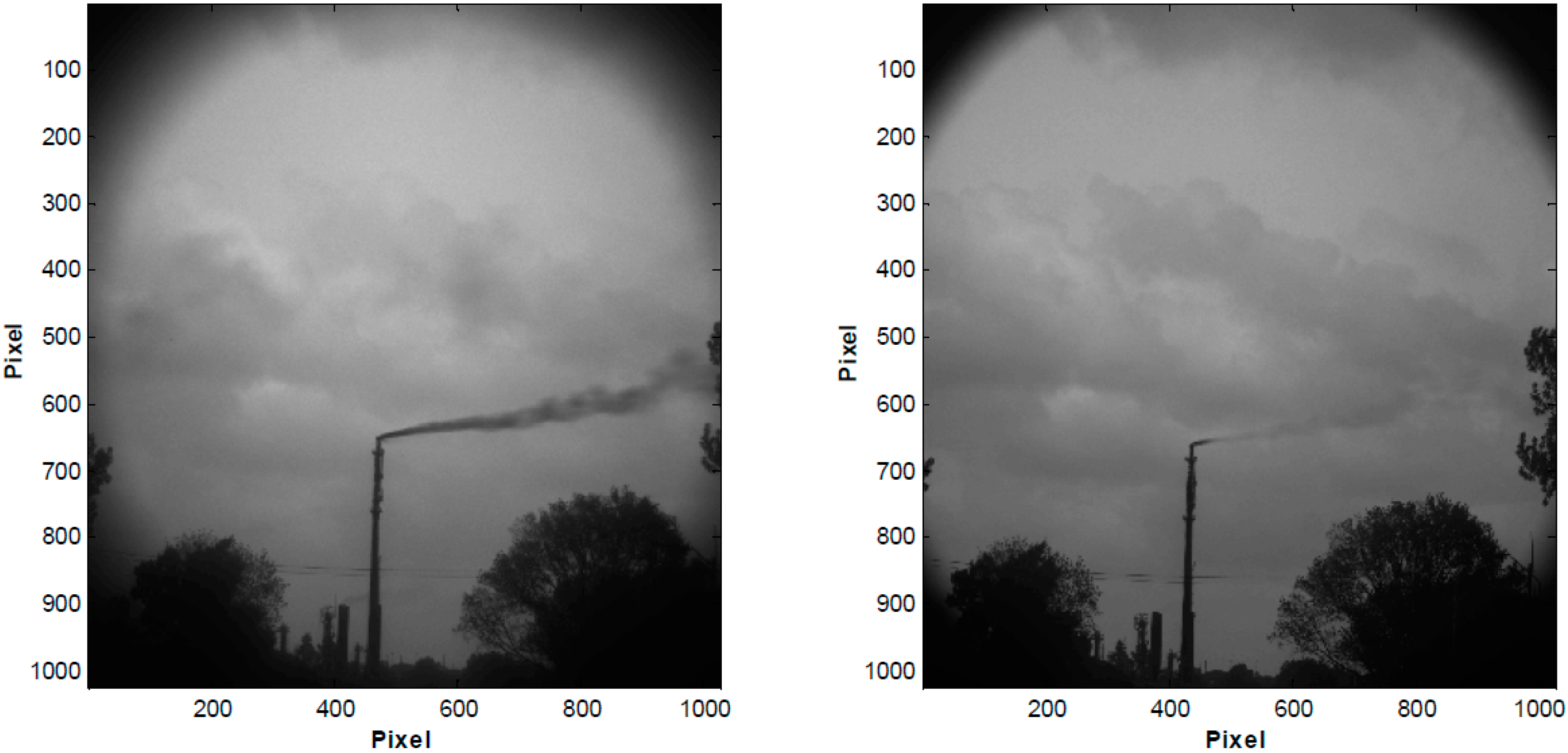
On 26 March 2015, between 10:46 and 12:04 local time, we acquired several hundred pairs of images of the plume emitted from a stack of the oil refinery with the UV cameras, as described in
Section 3.1. We adapted the exposure times in order to acquire images under different illumination levels due to changes in the solar zenith angle (SZA). The exposure times were selected in the range of 400 to 600 ms, and 200 to 450 ms, for 310 and 330 nm, respectively. This was done in order to obtain a good SO
2 signal, which corresponds to 60–80% of the intensity saturation level. Longer exposure times are required for the camera with the 310 nm band pass filter, due to the low intensity of the solar radiation and low quantum efficiency of the CCD at this spectral region. The internal temperature of the cameras was set to 10 °C. After the emission observations, the entrance optics was blocked in order to acquire dark current images and correct them before the evaluation process.
Figure 5 shows an example of a pair of raw images
I(
λ310,i,j) and
I(
λ330,i,j).
Then, we established correspondence between the pixels of the raw images
I(
λon/off,i,j), as described in
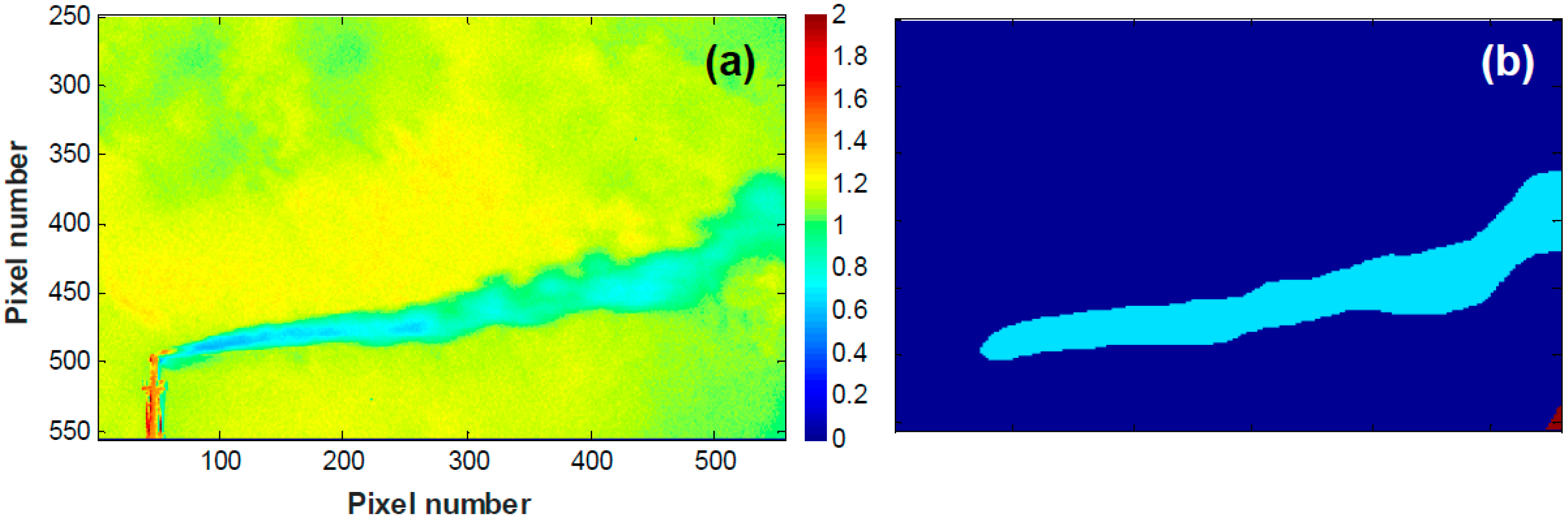
Section 3.2, and a spatial low-pass filtering was performed to remove some small artifacts from the images. Afterwards, we performed the quotient
I(
λon,i,j)/
I(
λoff,i,j) and selected a working region enclosing plume and sky to both sides of the plume, disregarding trees and image borders (
Figure 6a). By thresholding and labelling (Gonzalez and Woods [
23]), we located the plume spatial distribution (
Figure 6b). Due to the low-pass filtering and the posterior thresholding operation, the region occupied by the plume looks a little broadened, but this involves only a few pixels which do not affect the final results (emission rate calculation).
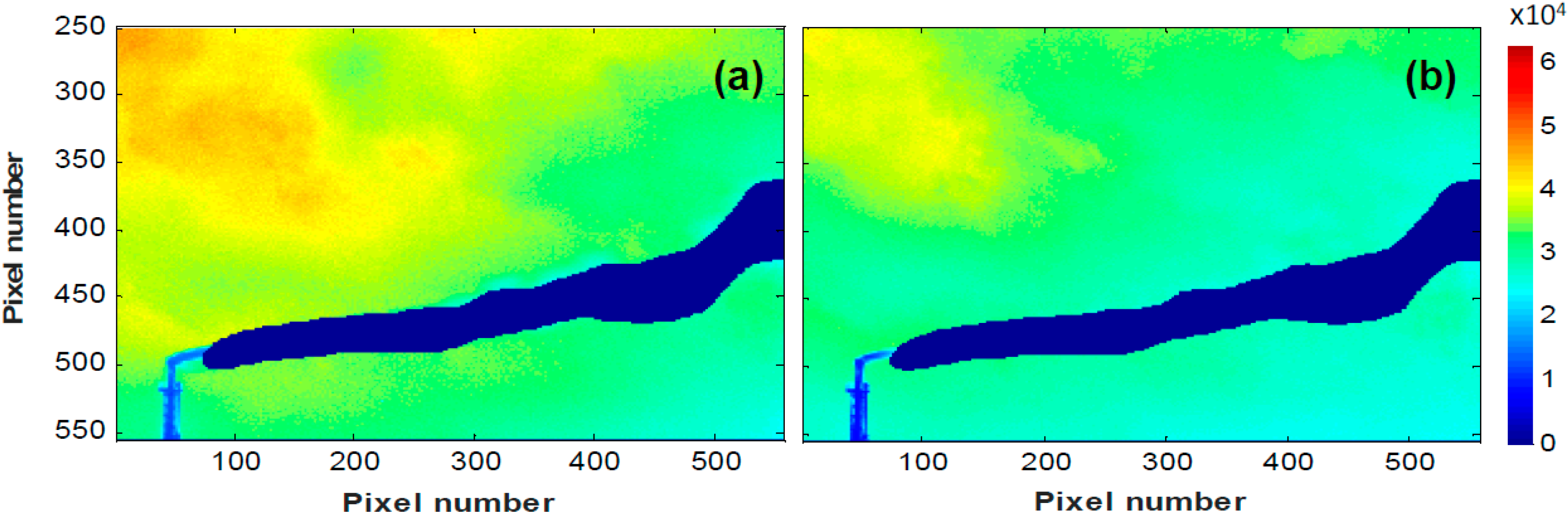
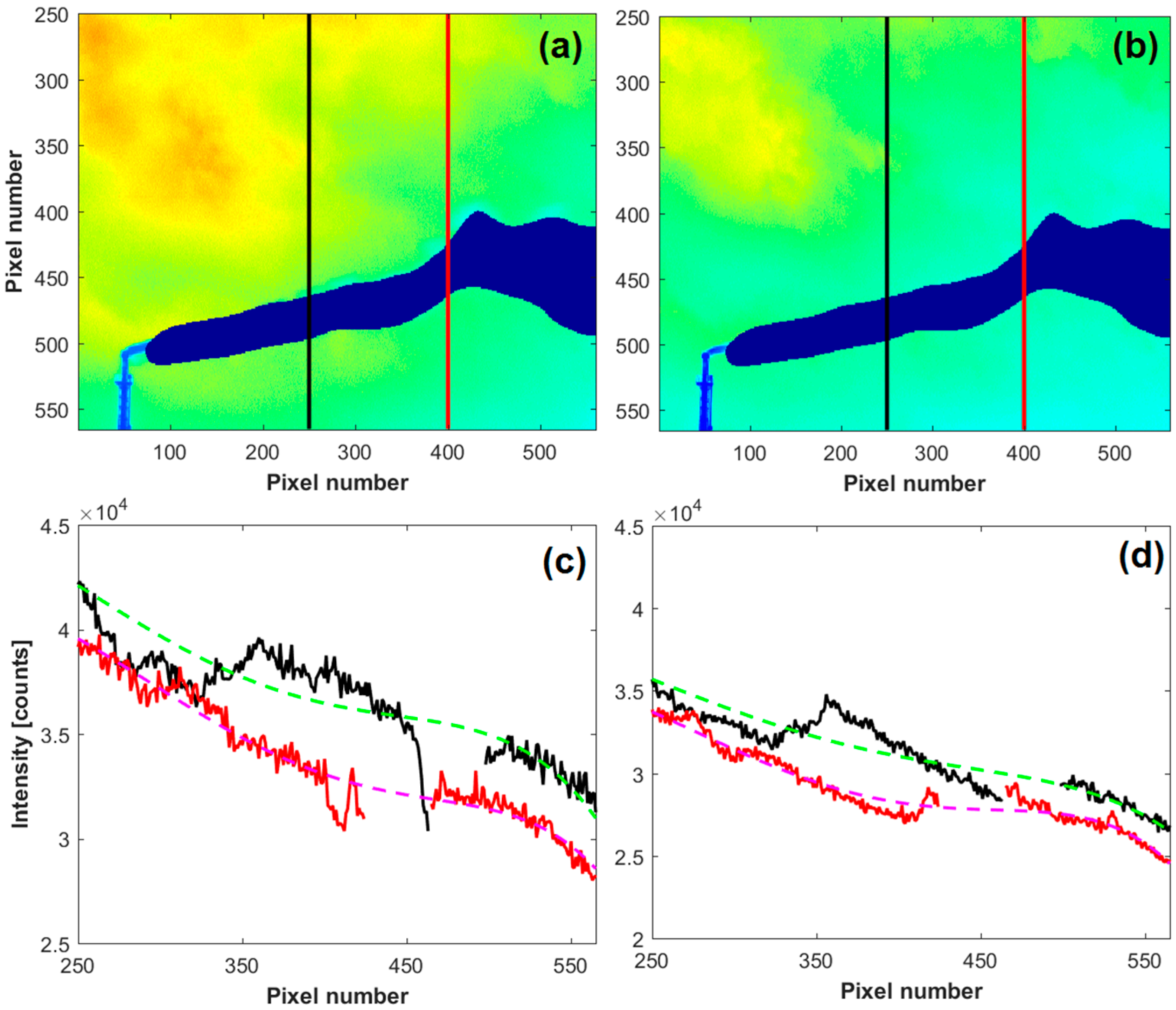
As a next step, the region occupied by the plume was removed (segmented) from the images
I(
λon/off,i,j) (see
Figure 7a,b). Then, we took vertical profiles at horizontal separations of one pixel, For every vertical profile without plume, a fifth-order polynomial fit (filling the gap) was applied that generated a sheet that approximates the background
I0(
λon/off,i,j), as mentioned in
Section 2.2 (see inlet in
Figure 2). This procedure is shown in
Figure 8.
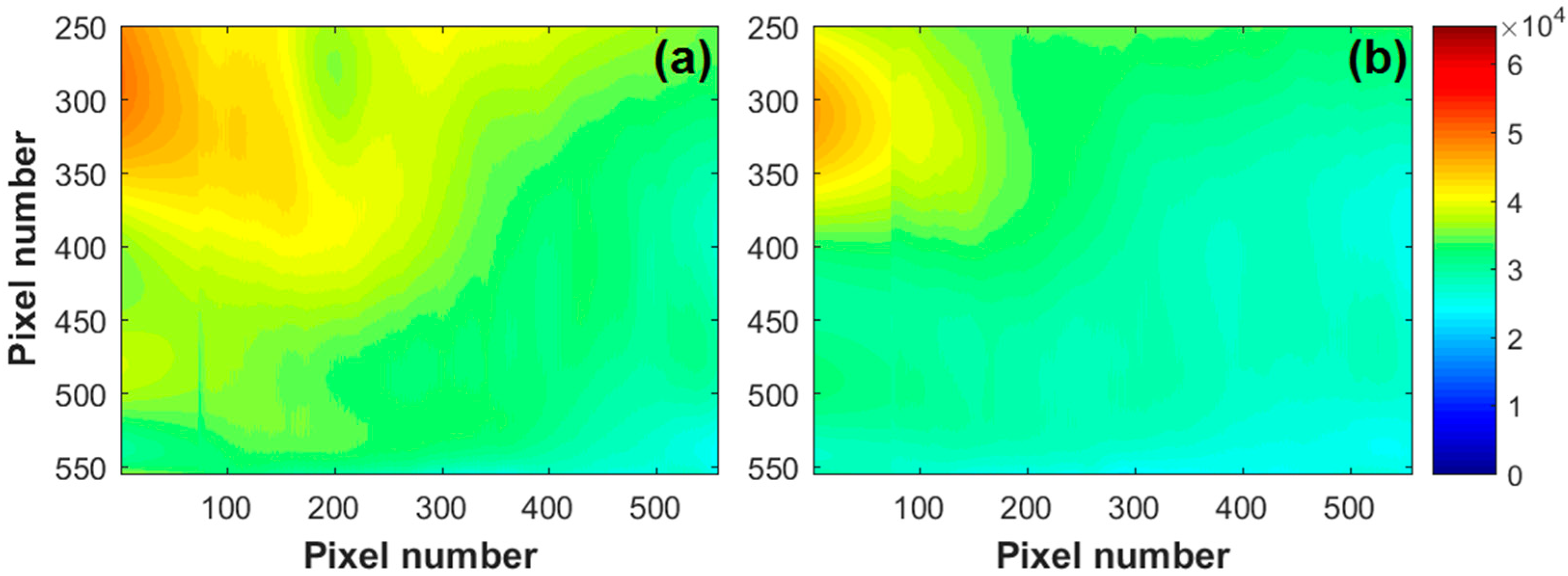
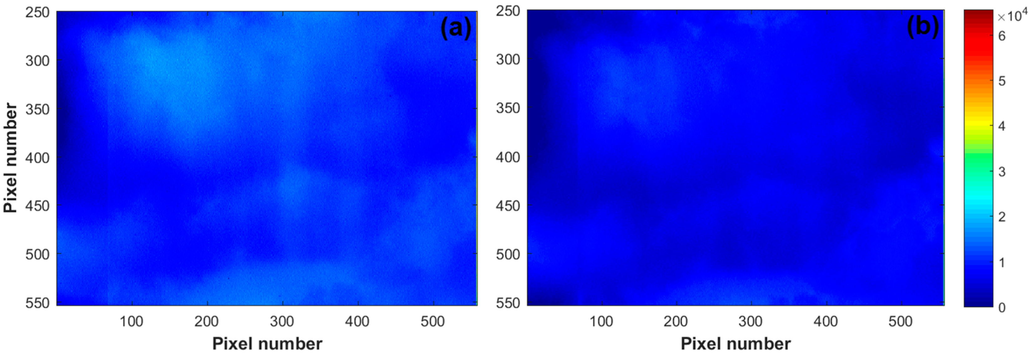
Figure 9a,b shows the generated artificial background images
I0(
λ310,i,j) and
I0(
λ330,i,j) resulting from the procedure described above. It is important to mention that the artificial background does not need to be recalculated each time. We want to retrieve an emission map, as long as the illumination conditions (or clouds) do not change. If this is not the case, i.e., clouds behind the plume move rapidly, in order to minimize the error in the retrieval process, the artificial background should be generated for each set of images.
On the other hand,
Figure 10a,b shows background images acquired by changing the viewing direction (~70° to the left of the stack), as required by the 4-IM method. Clearly, the background images acquired by varying the viewing direction do not match with the artificial background generated by the 2-IM procedure.
Figure 11 shows the subtraction between the background acquired changing the viewing direction and the background derived from the fitting process for each wavelength. Clearly, it can be seen different structures due to the clouds.
In order to retrieve a two-dimensional map of optical depth τSO2(i,j) (alternatively, the differential slant column density, dSCD, derived after a calibration procedure), in a first approximation, we will set (λoff/λon)α ≈ 1 in Equation (6).
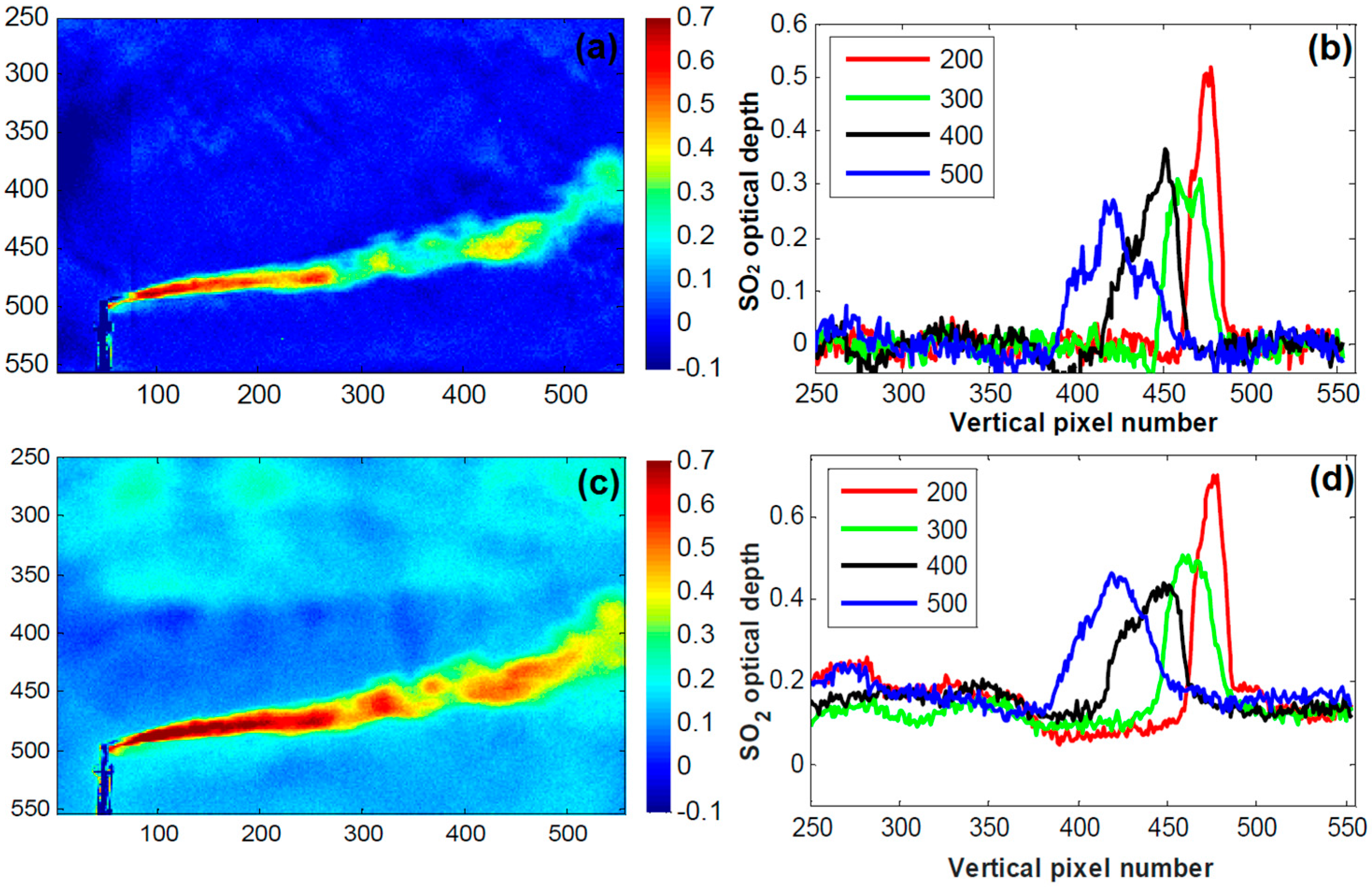
Illustrative examples of the two-dimensional emission maps obtained from Equation (6) by using the 2-IM approach are presented in
Figure 12a in false colour—SO
2-free sky (i.e., zero SO
2-concentration) is depicted in dark blue and high SO
2-concentration is depicted in red as shown in the scale on the right. The plots in
Figure 12b show vertical intensity cuts (optical depth
τSO2(
i,j)) across the plume at different horizontal positions.
Figure 12c shows the result obtained by the 4-IM method starting from the same raw images as before (
Figure 5), but now by using the background images shown in
Figure 10a,b.
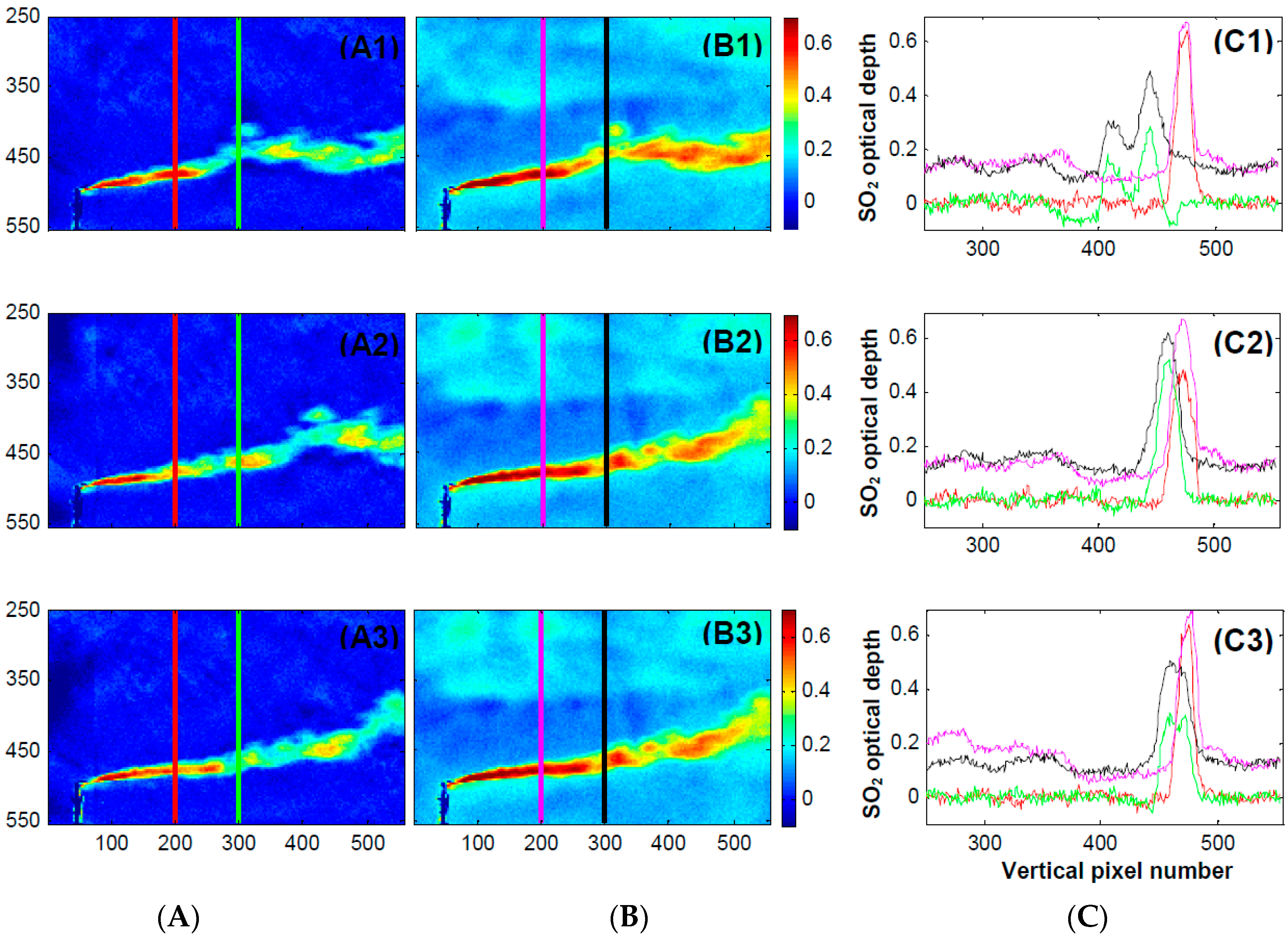
Figure 13 shows other examples of two-dimensional maps of SO
2 optical depths obtained from Equation (6) using the 2-IM and 4-IM approaches.
The comparison of
Figure 12 and
Figure 13A with
Figure 13B clearly show that the retrieved SO
2 optical depths obtained from both methods are quite different when clouds are present. For example, the artificial sky derived from applying the 4-IM procedure appears inhomogeneous and shows a large amount of spurious SO
2 optical depth outside the emitting plume. Meanwhile, the artificial sky obtained using the 2-IM procedure appears homogeneous and shows an optical depth near to zero as expected. Also, the peak values of the SO
2 optical depth at the plume are overestimated by the 4-IM method in a magnitude of 25–30%, with respect to the 2-IM ones.
4.1. Calibration and Detection Limit
In order to calculate the actual value of the SO2-emission rate of the stack, the two-camera system requires calibration. For the purposes of the present work, however, calibration plays a secondary role, since the relative performance comparison between 2-IM and 4-IM approaches can be done in terms of SO2-optical depth.
In order to estimate the SO2-density [ppm.m] from the measured optical depth (τSO2(i,j)), we performed calibration measurements using SO2-calibration cells containing 94, 480, 985 and 1740 ppm.m. After a linear fitting procedure, we estimate that a SO2-density of the order of 800 ppm.m corresponds to a value of τSO2(i,j) ≈ 0.3, which results from the linear calibration curve τSO2(i,j) = (3.7299 × 10⁻⁴) τSO2(i,j) [ppm.m]. The calibration was performed on a clear day (with a cloud-free sky).
The calibration uncertainty can be estimated by performing a characterization during different days and sky conditions (e.g., SZA and presence of clouds). We found that under different conditions, around midday, the calibration changes at most 20%.
The resulting optical depth (applying the 2-IM method) at image areas outside the plume will be considered as noise, for example, the rapid fluctuations outside the plume region in the plots in
Figure 12 and
Figure 13C. We estimated the detection limit of our measurements through the standard deviation of the noise, as discussed in [
4]. For the measurements performed on 26 March, the estimated detection limit was 47.5 ppm.m. This confirms that our system works well in conditions of relatively low emissions of industrial stacks.
4.2. Emission Rate Calculation
Assuming that the trace gases of the plume are transported at wind speed, the SO
2-flux can be calculated through the expression (Frins et al. [
25]):
where
is wind speed,
R the distance to the plume in the viewing direction,
is the normal to the plume cross-section, and
SSO2 is the SO
2 differential slant column density at the elevation angle
αi (in the interval of width Δ
αi).
Error sources in the emission rate calculation are due to: (1) uncertainties in the wind speed; (2) uncertainties in the determination of differential slant column densities, and (3) uncertainties in the determination of distance to the plume.
The wind direction was estimated by visual inspection of the plume, while the wind speed was estimated, on average, at 24.6 km·h
−1, derived from the movement of plume features in successively captured images. This, and other methods to determine the plume speed, has been used in similar systems [
21], and by ground based measurements with a single [
26] or multiple spectrometers [
27]. It should be mentioned that optical flow methods are accurate speed estimation tools, especially for turbulent plumes [
28]. We estimate an uncertainty of approximately 10% due to the wind speed. The error in the slant column density is partially due to the calibration process, and its estimated value is in the order of 4%. Potential errors derived from radiative transfer effects like light dilution were ignored, since we are dealing with distances to the plume in the order of 850–900 m (Kern et al. [
29]).
Finally, the distance between plume and observation site was estimated with the help of Google Earth, and its uncertainty was approximately 10% (estimated considering small changes by the wind direction). Thus, taking into account all the aforementioned uncertainties, we found an estimated error in the order of 20% in the emission rate. Certainly, the total error estimation will depend on the method utilized for generating the background, but it is difficult to quantify a priori its order of magnitude.
It is important to mention that for the calculation of emission rates, the crude SCDs obtained by the 4-IM procedure could not be utilized without—at least—a previous convenient compensation of the non-uniform intensity distribution in the picture. Thus, the results of the estimations of emission rates by the 4-IM procedure shown in
Figure 12c,d and
Figure 13B require some caution.
This problem practically does not occur in the 2-IM procedure, because the artificial background images are extracted from the proper emission images by applying a polynomial fit. Therefore, when some cloudiness is present in the sky, the construction of the background images utilizing the 2-IM method could produce a better retrieval of emissions, than by the 4-IM-method of pointing the camera in a different direction.
For the 2-IM procedure, emission rates between 162 ± 36 kg·h
−1 and 626 ± 140 kg·h
−1 were obtained. On average, an emission rate of 329 ± 74 kg·h
−1 was obtained.
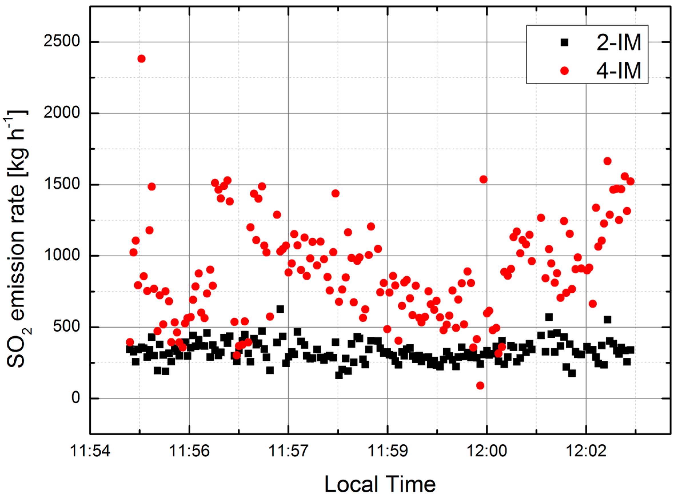
Figure 14 shows the results for the emission rates quantified by both methods. It is clear that the flux derived by 4-IM method is overestimated (the emission rate for this method was computed after a manually correction of the offset that is shown in
Figure 13C), showing a dynamic behavior along the measurement time. This is due to the changing of background conditions due to the presence of clouds. On the other hand, the 2-IM method shows an approximately constant behavior, coherent with the assumption of a constant work regime of the facility.
4.3. Comparison with MAX-DOAS Measurements
In order to validate the SO2 fluxes obtained using the 2-IM approach, we simultaneously performed measurements with a MAX-DOAS instrument (Hoffmann Messtechnik GmbH) from the same location where the cameras were placed. The instrument includes an Ocean Optics USB2000+ spectrometer, with a spectral range between 317 and 465 nm. The resolution varies in the range of 0.45–0.65 nm, and has a full field of view of approximately 0.8 degrees. The internal temperature of the instrument was set to 10 °C before starting the measurements, and we acquired a dark current and offset spectrum for correction at the end of the day.
To perform these measurements, the MAX-DOAS instrument was set to acquire spectra with an acquisition time of 30 s in a loop routine of elevation angles from 0° to 20° in 1° steps, 45°, and finally a zenith measurement, which was later used as reference in the DOAS evaluation. The whole plume cross section was completely scanned three times. During the measurements, the wind speed was 24.2 km·h−1 (derived from the images) and the sky was covered with clouds.
For the calculation of slant column densities, the WINDOAS software (Fayt and van Roozendael [
30]) was used. For the SO
2 analysis, the SO
2-cross section at 294 K (Vandaele et al. [
24]), O
3 at 243 K (Bogumil et al. [
31]), HCHO (Meller et al. [
32]), NO
2 (Vandaele et al. [
33]), a synthetic Ring spectrum calculated using DOASIS software (Kraus [
34]), and a fourth degree polynomial were included. The analysis window was set between 317 nm and 335 nm. Once the SO
2 slant column densities at different elevation angles crossing the plume were obtained, we proceeded to obtain the corresponding SO
2 emission rates.
With the MAX-DOAS instrument, were measured SO2-emission rates between 265 ± 59 kg·h−1 and 382 ± 85 kg·h−1. On average, we obtained an emission rate of the order of 315 ± 41 kg·h−1, which is consistent, within the experimental error, with the SO2-emission rate of 352 ± 77 kg·h−1 obtained by the 2-IM procedure.
5. Conclusions
In this work, we presented a new approach that uses background images constructed from emission images by an automatic segmentation and interpolation procedure to estimate the light intensity behind plumes. We also compared its performance with the four images method, which uses as background sky images acquired at a different viewing direction. Unlike other methods published in the literature (e.g., [
21]), we focus our efforts to present a non-iterative approach that locates the plume region in an acceptable way, trying to minimize user intervention.
We demonstrated that, even when clouds are present, the SO
2 emission rate derived by the 2-IM approach agrees, within the experimental error, with the results obtained by the MAX-DOAS measurements. This is not the case for the 4-IM approach due to spurious non-homogeneities in the images, which resulted from the comparison of different cloud structures. As can be observed in
Figure 14, the 2-IM method provides an emission rate that varies in the range of 160–626 kg·h
−1, while the 4-IM method primarily varies between 400 and 1500 kg·h
−1, in the same period of observation. The results obtained by 2-IM, agrees with the MAX-DOAS observation, which was on average in the order of 352 kg·h
−1.
It is important to note that, for evaluating emission rates by using the 2-IM procedure, two images less are needed than by the 4-IM method, which requires moving the cameras from their original position pointing in a new direction. As this direction selection is not always representative of the background, and also depends on the personal discretion of the user, it could lead to different results.
The 2-IM approach has the advantage that the cameras are always at rest pointing in direction of the SO2-emitting source, which is a necessary condition for acquiring an image sequence (i.e., a video) with the purpose of studying its temporal evolution. On the contrary, in the 4-IM procedure, the need of mechanical movement of the cameras may be a drawback in dynamical situations (e.g., background illumination changes due to the variation of the solar zenith angle, displacements of clouds behind the plume) in which the emissions and lighting conditions are changing with time.
Under stationary clear sky conditions, appreciable differences in the results obtained by both methods should not be expected. However, the change of viewing direction in the 4-IM approach also changes the relative sun position, which may lead to a kind of spatially variant offset in the emission results that should be corrected.
The 2-IM procedure requires certain additional software tasks, in comparison with the 4-IM. However, the computational cost is not relevant if we perform the image processing by, for example, using a GPU. The main assumptions of the 2-IM approach is that the light intensity on each side of the plume (right and left in case of a vertical plume, and above and below in the case presented here) is similar to that directly behind the plume, and that the plume cross section is small in comparison with the whole image.

