
Integrated System for Auto-Registered Hyperspectral and 3D Structure Measurement at the Point Scale


1
School of Instrumentation Science and Opto-electronics Engineering, Beihang University, Beijing 100191, China
2
Institute of Remote Sensing and Digital Earth, Chinese Academy of Sciences, Beijing 100094, China
*
Author to whom correspondence should be addressed.
Remote Sens. 2017, 9(6), 512; https://doi.org/10.3390/rs9060512
Submission received: 2 March 2017
/
Revised: 9 May 2017
/
Accepted: 21 May 2017
/
Published: 23 May 2017
(This article belongs to the Special Issue Earth Observations for Precision Farming in China (EO4PFiC))
Abstract
:Hyperspectral and 3D structure measurement are among the active research areas of remote sensing in recent years. The combination of these two kinds of information can provide improved outcomes distinctly, which is widely used in vegetation physiology, precision agriculture and radiative transfer modeling. However, the registration and synchronization has been overlooked in data acquisition. The mismatched characteristics have limited the potential application of the hyperspectral and 3D structure data as a complete data set. This paper proposes a laboratory prototype which can integrate the hyperspectral and 3D structure measurement at the point scale. The prism dispersion and laser triangulation ranging are performed in a common optical path as a result of the coplanar design of the critical optical devices. The hyperspectral data and depth data of the same object point are acquired from the same focal plane, which makes the data auto-registered spatially and temporally. Test experiment verifies the accuracy of the data provided by the prototype and the actual measurement experiment demonstrates the feasibility of the design in vegetation observation.
1. Introduction
Quantitative remote sensing has been a potential research area in recent years [1,2]. Hyperspectral and 3D structure measurement are among the active research techniques in quantitative remote sensing. The former provides rich spectrum that can reflect the biochemical information of the target and the latter provides detailed geometric information relating to the structural properties of the object. Both of the two techniques have been widely applied in vegetation physiology [3], precision agriculture [4], radiative transfer modeling [5], etc.
It has been proved that the integration of hyperspectral data and 3D structure data provides improved outcomes distinctly over use of either data set alone [6,7]. Some researchers have studied the application of the integration and various instruments have been proposed to combine the two techniques to realize an integrated measurement. Kalisperakisa et al. carried out a leaf area index (LAI) estimation in vineyard using hyperspectral data, 2D images and 3D canopy surface models [8]. They generated a 3D model from the images by employing dense stereo and multi-image matching algorithms. The experiment result demonstrated that LAI was estimated more accurately from the hyperspectral data and 3D canopy model. Asner et al. proposed an instrument named Carnegie Airborne Observatory (CAO) to conduct in-flight fusion of hyperspectral imaging and light detection and ranging (LiDAR) [9]. The two kinds of data were registered with a precise ray tracing process with the root-mean-square position uncertainty less than 0.15 m and they applied CAO in the studies of ecosystems and narrowed the solution domain for a variety of integrative products such as growth rates. Aasen et al. generated 3D hyperspectral information with unmanned aerial vehicle (UAV) snapshot cameras for vegetation monitoring [10]. The hyperspectral images were matched with the grayscale images and the 3D information was also derived from the grayscale images with the structure from motion (SfM) algorithms. Behmann generated the hyperspectral 3D plant models from the data provided by the hyperspectral pushbroom cameras and 3D laser scanner [11]. The cameras and laser scanner were calibrated in a unique coordinate system to fuse the hyperspectral images and 3D data. Avbelj conducted the coregistration refinement of hyperspectral images and digital surface models (DSM) provided by LiDAR by matching the object features extracted in the two data sets and estimating the transformation parameters [12]. Liang performed a 3D plant modelling via hyperspectral imaging [13]. The hyperspectral images were firstly used to segment plant from the background and the 3D model was then directly built from a sequence of hyperspectral images with the SfM algorithms.
For existing researches, the combination of the hyperspectral and 3D measurement can be summarized in two categories. The first one is a kind of instrument which acquires hyperspectral and 3D data with different sensors. In general, the hyperspectral data is usually provided by pushbroom or snapshot cameras and the 3D data is usually provided by LiDAR, laser scanners or derived from grayscale images. The two kinds of information are integrated with various fusion algorithms after the data is acquired. The drawbacks of this category are obvious, that it is a tedious work to register data from different sensors and it often relies on extra information. For example, the ray tracing process for the hyperspectral images and 3D data from LiDAR should be conducted pixel by pixel and it requires high precision Global Positioning System & Inertial Measurement Unit (GPS-IMU) navigation and trajectory analysis of the instruments onboard the aircraft [9]. As another example, the fusion of hyperspectral data and 3D data derived from different cameras requires a precise calibration process to be unified in a same coordinate system [14,15]. Furthermore, data acquired from different sensors is often provided with different resolutions, which means that one should sacrifice its resolution to match with the other. Another category is to derive 3D data directly from the hyperspectral images with the computer vision methods. This category does not need a data fusion process but it requires sufficient matching information to conduct the 3D reconstruction [16]. Due to the low quality of the hyperspectral images, it is difficult to extract enough features, which limits the accuracy of the 3D data.
As mentioned above, there hasn’t been an instrument that can provide physically registered hyperspectral data and 3D data. If these two kinds of data can be acquired from a single sensor simultaneously in time and space, the registration will be highly precise and the data set can be applied directly without any fusion process.
In this paper, we propose an integrated prototype which combines hyperspectral and 3D structure measurement at the point scale. This prototype can provide a dense 3D point cloud of the measured object, and for every point in the cloud, a physically registered spectral curve is also provided. To the best of our knowledge, it is the first time that such a system is reported with the ability to conduct an auto-registered hyperspectral and 3D structure measurement spatially and temporally.
2. Background and Prototype
2.1. Background
2.1.1. Principle of Prism Spectrometer
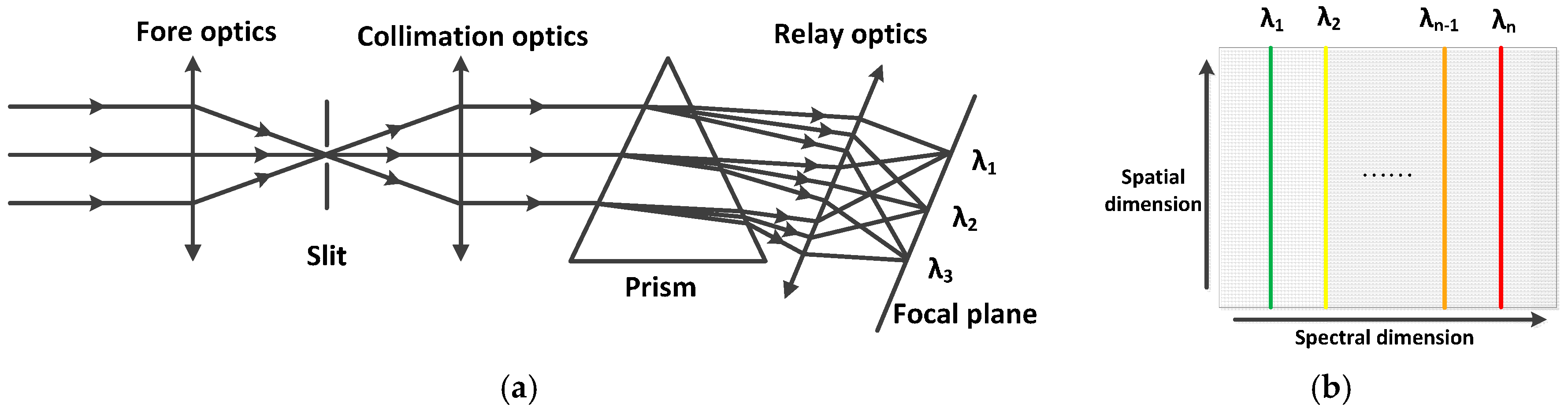
Figure 1a exhibits a schematic of a typical prism spectrometer [17]. The incident light is imaged by the fore optics onto the primary imaging plane where lies a slit as a field diaphragm. Light passing through the slit reaches the first refraction surface of the prism after collimated. The prism is the core dispersion component of the spectrometer. According to the refraction principle, the outgoing light has a larger deflection angle for the shorter wavelength. After passing through the prism, the output light is imaged by the relay optics and spread out on the focal plane sequentially according to the wavelengths.
Figure 1b illustrates the raw image on the focal plane in a prism spectrometer. The horizontal direction is the spectral dimension and each position represents a certain band of the wavelength. The vertical direction is the spatial dimension and each position represents a specific location of the object point.
2.1.2. Principle of Laser Triangulation Ranging
Figure 2a illustrates a simple laser triangulation ranging system consisting of a laser as the launching device and a camera as the receiving device [18]. Laser beam emitted from the launching device illuminates the object point. The reflected beam is imaged by the camera with the image point recorded on the focal plane [19]. Given the geometric parameters of the ranging system, the depth information of the illuminated object point can be calculated with Formula (1):
where d is the distance between the object point and the baseline, which is often designated as the concept “depth”; L is the length of the baseline; is the angle between the emitted laser beam and the base line and is the angle between the reflected beam and the base line.
Figure 2b is the enlarged image of the camera in Figure 2a. The reflected beam is imaged on the focal plane after passing through the principal point of the camera. Given the intrinsic parameters of the camera, the angle is described as Formula (2):
where f is the focal length of the camera and is the physical size of a pixel. Combining Formula (1) and Formula (2), the depth d is calculated:
It can be seen from Formula (3) that the depth of the object point is a function of the coordinate of the image point. It should be noted that, for the reason of a simpler presentation, the pixel coordinate axis is parallel to the baseline in Figure 2b, while the one-to-one mapping between the depth and the image coordinate still remains even when the parallel relationship no longer exists. In the actual measurement, it is difficult to get the accurate geometric parameters of the measuring system as a result of the machining and alignment errors. Therefore, the relationship between d and N is often obtained with an accurate calibration process. Thus, Formula (3) is simplified as:
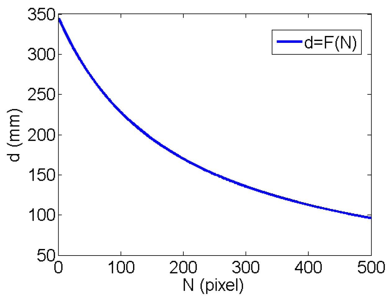
Figure 3 illustrates the simulation result of Formula (3)/(4). Once the image coordinate of the laser point is obtained, the depth value is acquired. As can be seen from Figure 2b, if the origin of world coordinate system O-xyz is located at the principal point of the camera with the z axis parallel to the optical axis, the acquired depth value d can be designated as the z coordinate of the object point. If the x and y coordinates can be provided with other methods, such as an additional XY-stage, the 3D coordinates of the object point is determined. It should be noted that to obtain the depth of the object point with Formula (4), the major problem is to guarantee that the laser beam, the baseline and the optical axis of the camera lie in a certain plane. This problem is discussed in the next subsection.
2.2. Prototype Design
The principle of the prototype design is to integrate hyperspectral and 3D structure measurement with one single sensor to realize an auto-registered data acquisition process.
From the preceding part of this paper, both the prism spectrometer and the laser triangulation system need a camera as a receiver. The difference is that the former needs a two-dimensional focal plane while the latter needs a one-dimensional receiver. In the prototype design, from the focal plane of the prism spectrometer we leave an extra zone that acts as the pixel coordinate axis of the laser triangulation. Thus, the depth information and the hyperspectral information of the same object point are acquired from the same focal plane. With the other two-dimensional position information provided by the auxiliary motion mechanism, the depth data is upgraded into 3D coordinate. To realize this design philosophy, three primary problems are discussed in this section:
- common optical path design of spectral dispersion and laser triangulation ranging;
- separation of spectral dispersion and laser triangulation ranging;
- extraction of the auto-registered data.
2.2.1. Common Optical Path Design
In a prism spectrometer, the slit cuts the field of view (FOV) with a narrow strip left. Only object points falling in the narrow field of view can be imaged by the camera. In order to use the focal plane of the spectrometer to conduct laser triangulation ranging, the emitted laser beam must fall exactly into the narrow strip field of view at different depth. This constraint requires that the emitted laser beam, the optical axis of the fore optics and the slit of the spectrometer lie in the same plane. The coplanar property is illustrated in Figure 4.
Under the coplanar condition, the reflected laser light must pass through the slit. In other words, the narrow strip containing the object point illustrated by the laser beam will be imaged by the fore optics to the slit that lies on the primary imaging plane. The slit is then imaged by the relay optics after collimation and dispersion. The final images are spread out on the focal plane sequentially according to the wavelengths. The image of the laser point can be found along one column of the focal plane, which is the position that lies the component of laser wavelength.
This coplanar design guarantees that the spectral splitting and laser triangulation ranging use a common optical path and share one focal plane to acquire data. Thus, the hyperspectral data and the 3D data are acquired synchronously at the data source and are physically registered.
2.2.2. Separation of Spectral Dispersion and Laser Triangulation Ranging
As the hyperspectral data and 3D data are acquired from the same focal plane of a camera, they should not interfere with each other.
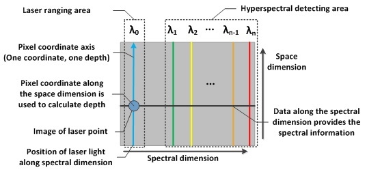
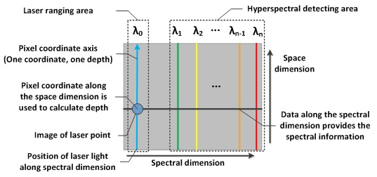
The dispersion area of the spectrum is firstly designated according to the design index of the hyperspectral measurement. The camera is then selected with a bigger photosensitive area on the focal plane. Thus, the prism spectrometer leaves an extra zone for the laser ranging area. As shown in Figure 5, the right part of the focal plane is used to conduct the hyperspectral detecting and the left part is used to conduct laser ranging. Due to the coplanar property mentioned above, the laser light is imaged only on the specific column of the focal plane, which is designated as the pixel coordinate axis. Therefore, the hyperspectral data and 3D data will not interfere with each other.
2.2.3. Extraction of the Auto-Registered Data
Although the location along the spectral dimension is fixed, the position of the imaged laser point in the spatial dimension varies with the depth of the object point. The coordinate of the laser point on the pixel coordinate axis is firstly extracted, then the auto-registered hyperspectral data and 3D data are acquired with the following procedures:
- (a)
- The depth value d is calculated with Formula (4) and is designated as the z coordinate in the world coordinate system O-xyz.
- (b)
- The x and y coordinates are recorded by the extra auxiliary motion mechanism. Thus, the 3D coordinates of the object point is determined.
- (c)
- With the pixel coordinate fixed along the spectral dimension, extract data on the same line of the focal plane along the spectral dimension, as shown in Figure 5. This data is the spectrum that corresponds to the exact object points where the laser illuminates.
Thus, the hyperspectral data and 3D data are physically registered from the same focal plane. In fact, the laser triangulation ranging only detects one single point at each measurement. However, the prism spectrometer has a line field of view containing a large number of object points in the measurement scene. As mentioned above, on the focal plane only the spectral data on the same line with the laser point is extracted with the rest of the data abandoned. The reason is that for the other area on the focal plane, there are no corresponding laser points. It means that although the spectrum of the other object points can be acquired, the 3D information cannot be provided. This sacrifice of spectral data is a compromise for the design philosophy of physical registration.
As the prototype only acquires data of a single point at one time, to obtain the whole 3D and hyperspectral information of the object, an auxiliary motion mechanism is required to realize the relative scanning motion between the prototype and the object. Figure 6 shows the schematic map and photo of the completed prototype.
2.3. Prototype Calibration
Before the practical measurement, the prototype needs an accurate calibration. The primary objective is to obtain the relationship between the wavelength and the pixel coordinate along the spectral dimension and the mapping between the depth and the pixel coordinate along the spatial dimension.
2.3.1. Spectral Calibration
The spectral calibration is performed with a monochromator which is a production of Princeton company with the major parameters listed as Table 1:
The monochromator is used to provide the standard source of the spectrum within the spectral range of the prototype with a drive step size of 1 nm. During the scanning process, the laser is closed. At each step, the corresponding narrow strip image on the focal plane is recorded and the pixel coordinate along the spectral dimension is calculated. When all the spectral images are acquired, the relationship between the pixel coordinate and wavelength is obtained with a fitting method. The spectral resolution of the prototype is also calculated with a technique commonly used in [20,21]. The spectral calibration is conducted at a very close range of 250 mm to match the working distance of the prototype. Under this circumstance, the atmospheric effect on the spectrum can be neglected.
2.3.2. Depth Calibration
The depth calibration is performed with an electric displacement platform, which is a product of Zolix company with the positioning accuracy of 30 µm. The platform is moving along the depth direction of the prototype within the depth range with a drive step of 10 mm. During the scanning process, the laser is opened. At each step, the corresponding image of the laser point is recorded and the pixel coordinate along the spatial dimension is calculated. Finally, the mapping between the depth and the pixel coordinate is obtained with a fitting method.
After a careful calibration process, the entire parameters of the prototype are listed as Table 2. It should be noted that, in the actual measurement, the pixel size is smaller than the laser point size at the working distance. Meanwhile, the coordinate of the laser image point is calculated in subpixel with the center extraction algorithm [22], so the actual size of the single point at each measurement is determined by the pixel size at the working distance.
3. Experiment and Results
3.1. Test Experiment
To verify the validity of data acquired by the prototype, a series of test experiments are carried out. In the spectral test measurement, the spectral curve of the same vegetation is acquired by the prototype and the Analytical Spectral Device (ASD), respectively. The comparison between the two curves is discussed. Then, the spectral curves of different vegetation are acquired by the prototype and data analysis shows that the spectral curves can reflect the different health status.
3.1.1. Spectral Measurement
A pepper seedling is selected as the measured object. This experiment is conducted in the laboratory condition with a tungsten halogen lamp as the light source. The lamp is positioned at a fixed location and the reference spectrum is firstly acquired with a standard diffusing reflector to convert the raw spectral data into the spectral reflectance. Then, the hyperspectral data of the seedling is acquired by the prototype with an ASD spectroradiometer recording the same area. Both the ASD spectroradiometer and the prototype conduct several measurements and export the mean values as the output data so that the random noise is reduced significantly and the spectral curve becomes smooth. Photos and results of the experiment are shown in Figure 7.
The relative error is calculated with Formula (5):
where Errorn is the reflectance relative error of band n, Rp is the reflectance provided by the prototype and RA is the reflectance provided by the ASD spectroradiometer. From Figure 7d,e, the two curves remain consistent in the general trend along the spectral dimension; meanwhile, there still exists obvious deviations in several bands. The influencing factors leading to the deviations are discussed as follows:
(1) Measurement errors brought by the stray light
As an engineering model of the first generation, this prototype aims at verifying the design of auto-registered measurement. The optical and mechanical structure is made simplified. Thus, the prototype shows obvious drawbacks in the stray light controlling. After several refraction and reflection on the optical and mechanical surfaces of the prototype, the unwanted stray light interferes with the effective signal on the focal plane finally. This is the main reason that leads to the deviation of the two curves. The stray light controlling is also one of the major problems that need to be solved in future work.
(2) Measurement errors due to the low quantum efficiency of the camera at the near infrared bands
The model of the camera used in this prototype is HK-A5100-GM, which is a product of Microvision Company. The nominal spectral range of this camera is 400–1100 nm. However, the quantum efficiency after 850 nm is lower than 15%, which makes the signal more easily influenced by the noise and stray light mentioned above. As a result, the prototype exhibits a poor performance at the near-infrared bands. This feature should be taken into account in the actual measurement and also in the future work.
(3) Measurement errors brought by different sampling points
The ASD spectroradiometer has an FOV of 25° and covers a small area of the measured object. Thus, the ASD spectroradiometer in fact provides a mixed spectrum. Meanwhile, the prototype provides spectrum of a single point at one measurement. The reflectance curve in Figure 7d is a mean value of several sampling points. Although the sampling points are selected within the measurement area of the ASD spectroradiometer, the difference between mixed spectrum and mean value of several single point spectra must not be ignored.
(4) Measurement errors brought by reflection property based on Bidirectional Reflectance Distribution Function (BRDF) of the measured object
As mentioned above, the ASD spectroradiometer observes the object with an FOV of 25°. Thus, different points in the covering area show different directions and the final data is a mixed spectrum. Meanwhile, the prototype is driven by an auxiliary motion mechanism with a translational motion. The normal directions of different sampling points vary with the orientation of the leaf. As a result of the BRDF of the leaf, the energy of the reflection light exhibits a deviation between the two measurements.
The four influencing factors mentioned above lead to the deviation between the two curves in Figure 7d. In the spectral range of 500 nm to 700 nm, the effective signal is relatively lower, so the measurement error occupies a larger proportion even though its absolute value is small. In the range of 700 nm to 900 nm, the relative error is smaller as a result of the higher effective signal.
In general, the spectral data provided by the prototype can reflect the trend along the spectral dimension. However, the measurement error of the absolute value cannot be ignored. This problem should be considered in future work.
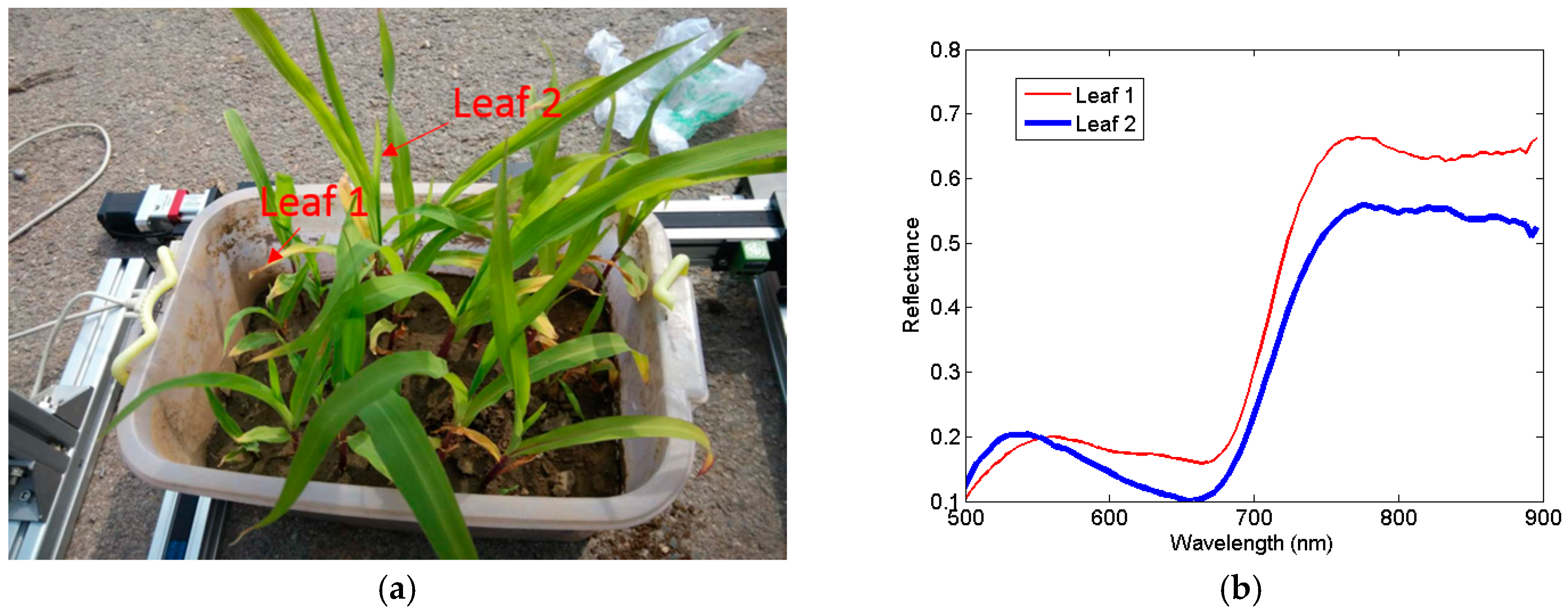
In addition to the comparison experiment, another spectral experiment is conducted. A cluster of maize seedlings under low nitrogen stress is selected as the measured object. During the growth, the seedling accumulates the rare nitrogen in new leaves. Old leaves are under unhealthy growth status due to the lack of nitrogen, which is the raw constituent of chlorophyll. As shown in Figure 8a, Leaf 1 is an old leaf with a yellow color and Leaf 2 is a new leaf with a normal green color. Figure 8b shows the spectral curves of the two leaves acquired by the prototype. It can be seen that the reflectance of Leaf 1 is higher and the peak and trough of the curve move towards the longer wavelength with an obvious decrease in the contrast ratio in the peak–valley value, which are the typical features of nitrogen deficiency [23]. This test experiment indicates that the prototype can reflect the different health status of the vegetation.
3.1.2. 3D Structure Measurement
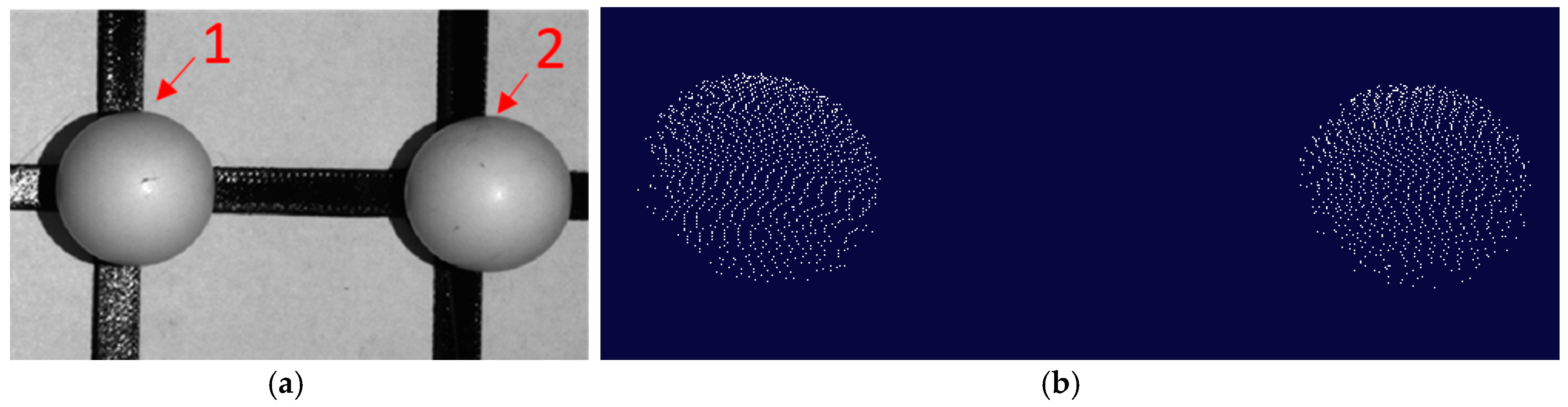
A 3D structure scanning experiment is carried out to test the accuracy in the actual 3D measurement. Two standard spheres are measured with a small scanning step of 0.5 mm to obtain a dense 3D point cloud, as shown in Figure 9. The measured diameter of the spheres are acquired with a spherical surface fitting method. Deviation between the measured value and the nominal value reflects the measurement error. The result of the measurement is shown in Table 3 and the measurement error at a distance of 250 mm is less than 0.4 mm.
3.2. Vegetation Measurement
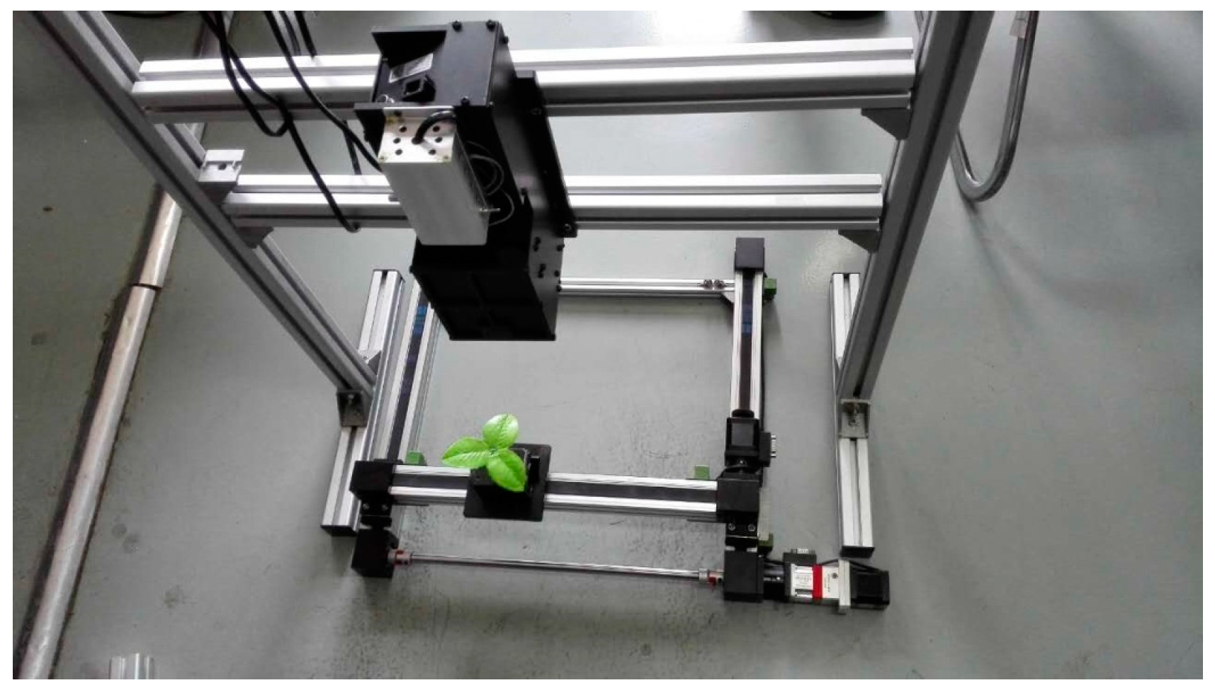
The actual vegetation measurement is conducted to demonstrate the auto-registration ability of the hyperspectral and 3D structure measurement, which is the primary design objective of the prototype. As mentioned in the preceding section, the prototype obtains the 3D coordinates and hyperspectral data of a single object point at one time. The whole measurement of a plant takes a scanning process. The prototype is moving with the auxiliary motion mechanism to realize the relative scanning motion under the laboratory conditions, as shown in Figure 10.
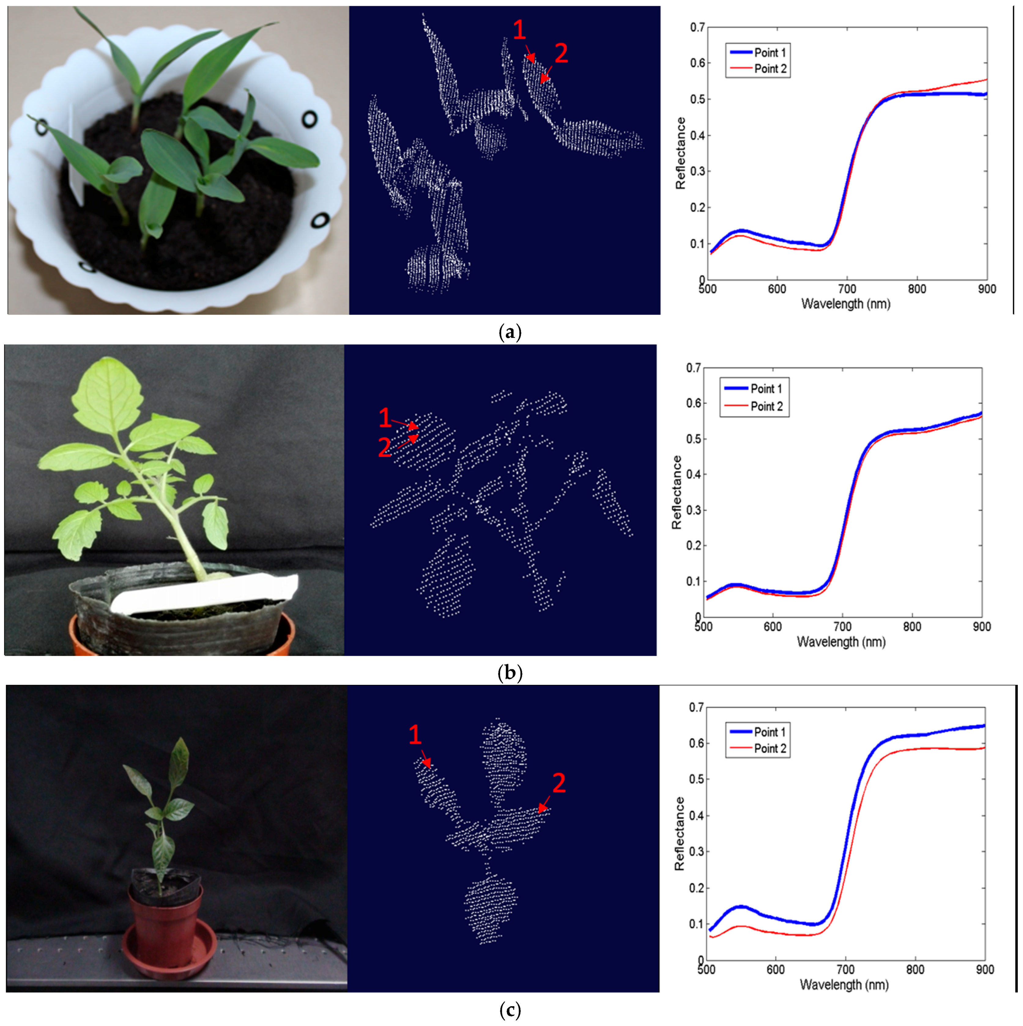
Different kinds of vegetation are measured and the 3D point cloud of each plant is acquired with a set of spectral data corresponding to every 3D point. Figure 11 shows the results of the maize seedling, the tomato seedling and the pepper seedling. From left to right in each sub-figure, the pictures are the color images, 3D point clouds and spectral curves of different points of the vegetation, respectively. There is some glitch noise attached to the origin measured spectrum, so we applied the Savitzky–Golay algorithm to smooth the spectral curve [24].
It can be seen that the proposed prototype can provide a set of hyperspectral and 3D structure data which is physically registered at the point scale. The 3D point cloud can describe the geometric information of the vegetation precisely and the spectral curves can distinguish the different parts of the vegetation sensitively, which verifies the feasibility of the design and the validity of the prototype.
4. Discussion
4.1. Application Ability of the Prototype
Obtained from the same focal plane, the hyperspectral and 3D structure data are physically registered. The auto-registered characteristic will bring much convenience to the application of the data set. Firstly, it does not require any fusion process, such as the spatial transformation of the data. Secondly, the hyperspectral and 3D data are point-to-point registered with the same resolution and do not need a resampling process. Thirdly, the synchronization in time can be used in many specific applications. For example, when the object is moving or if the crop is swaying with the wind, it is difficult for instruments equipped with different sensors to provide combined data of the same area. However, the hyperspectral data and 3D coordinates of the measured point provided by this prototype are still registered. Finally, the precisely matched characteristic can be used to extract more accuracy parameters for many applications. For example, with the 3D point cloud obtained of the plant, the leaf inclination angle can be calculated precisely, which can be used to correct the BRDF effects point by point. Thus, the high accuracy spectral reflectance can be acquired.
As specific examples, the prototype is compared with the instruments mentioned in previous work to illustrate the auto-registered characteristic. Compared with the image matching algorithms, which match the hyperspectral images with the RGB images [8] or grayscale images [10] and extract 3D canopy models by employing dense stereo and multi-image matching algorithms, the prototype does not need any image matching process, which avoids a large amount of computation. Some researchers register the hyperspectral data and 3D data with the precise ray tracing process, which requires high precision GPS-IMU navigation and trajectory analysis of the instruments onboard the aircraft [9]. Other researchers integrate the two data sets by calibrating the spatial location of different sensors and projecting different data into the same coordinate system [11]. However, in this prototype the prism dispersion and laser triangulation ranging are performed in a common optical path, so the spectral information and depth information come from exactly the same object point and data is acquired from the same focal plane. It means that the ray tracing process and the spatial projecting are physically conducted by the optical elements and the data set is auto-registered. Some studies extract image feature information from the hyperspectral images to match with the 3D data [12] or conduct computer vision process [13] to calculate 3D information. However, the matching accuracy is limited because it is difficult to find sufficient features due to the low quality of the hyperspectral images. In this prototype, the spectral data and the 3D data are registered at the point scale due to the common optical path design. In addition to the superiority, the obvious drawbacks of the prototype compared with the previous work are the very short working distance and the very slow measuring speed in the present situation, which should be considered in future work.
In general, we believe that the auto-registered hyperspectral and 3D measurement is an attempt to enrich the existing observation methods in quantitative remote sensing and it will have a great potential in many application domains.
4.2. Limitations of This Study
Although we performed some experiments and verified the feasibility of the design to some extent, this instrument still has some obvious limitations as a prototype of a first edition. The limitations are listed as follows:
(1) The spectrum accuracy needs to be promoted
Compared with the ASD spectroradiometer, the prototype presents a distinct error. This error mainly results from the stray light of the instrument and the low quantum efficiency of the camera at the near infrared bands. To improve the spectrum accuracy, stray light suppression methods should be introduced. For example, lens hoods can be placed at the critical positions and a higher photosensitive sensitivity device is required to replace the existing camera.
(2) The structure and parameters need to be optimized
The prototype uses a prism as the dispersion device and the spectral range of the prototype is 500–900 nm. As is known, the light decomposed from the prism has a nonlinear distribution, which limits the quality of the extracted spectrum and has a lower utilization ratio of the camera focal plane, while the grating splitting has a linear distribution with a higher diffraction efficiency. Therefore, a grating can be used in this prototype to replace the prism, which can provide a wider spectral range and spectrum with higher quality.
The prototype works at a distance of 150–300 mm with the depth range of 150 mm. This short distance will limit the use of the instrument in many applications. The structure of the prototype can be optimized to get a larger baseline for the laser triangulation so that it can work at a long distance with a larger depth range.
The point-by-point scanning mode with the auxiliary motion mechanism results in a very low measuring speed. One of the possible improved methods is to equip this prototype with an angle encoder to move the laser point along one direction. The angle encoder does not destroy the coplanar design of the prototype. Meanwhile, the prototype only needs to be moved along the other direction to realize the scanning process, which will improve the measuring speed distinctly.
(3) More application experiments need to be conducted
Restricted by experiment conditions and current state of the prototype, the experiments in this paper are mainly performed at a very close range in the laboratory condition. A small amount of tested objects and sampling points could not explain the common problems in detail. For example, the difference between the two spectral curves in Figure 8b is certainly a result of the different nitrogen contents in the two leaves. However, the spectral curve extracted from the single point is also easily influenced by the other factors, such as the shading of other leaves. Therefore, more experiments with various objects and a large number of sampling points are needed to provide a more persuasive result and find other application problems of the instrument.
4.3. Future Work to Apply the Instrument in Precision Agriculture
The registered hyperspectral and 3D data can provide biological, biochemical and structural information for the crop, which can be used in many applications of agriculture. One of the primary objectives of the proposed instrument is to be applied in precision agriculture. Therefore, improvements are required in future work.
Firstly, several parameters such as the spectral range and the working distance mentioned above should be adjusted to satisfy the agriculture requirements. In addition, the angle encoder can be applied to improve the measuring speed and the data acquisition mode can be optimized. In the laboratory research, the point-to-point matching characteristic is concerned, while in the precision agriculture application, data acquired from a larger scale will be more important. Under this circumstance, the instrument can return a mean depth value of several sampling points with the help of the angle encoder, which can be used to calculate the average plant height. In the preceding part of this paper, we mentioned that much spectrum data on the focal plane is abandoned with only one point left corresponding to the laser point. However, in the precision agriculture application, the whole spectrum can be retained. Therefore, the instrument can provide the average plant height and spectrum along a line field at each measurement. With a push broom process, it can cover a large area.
Secondly, the working conditions in field work should be considered. The power and wavelength of the laser should be carefully designed to guarantee that the laser point can be clearly imaged under the sunlight. The sensitivity of the camera and reflectivity of the crop should be considered to maintain the response of the camera at an appropriate level for data extraction. The other factors like the temperature, power supply and weather conditions should also be taken into account.
Finally, the platform is an important issue. In the laboratory, the prototype is driven by the auxiliary motion mechanism, while in the precision agriculture application, the instrument may be onboard the UAV or Unmanned Ground Vehicle (UGV). The data acquisition mode such as the measuring speed should match the motion pattern of the platform. Furthermore, location is also a pivotal problem in the measurement and the instrument should leave a specific interface to get access to the positioning system of the platform.
5. Conclusions
This paper proposes a laboratory prototype which can carry out a spatially and temporally auto-registered hyperspectral and 3D structure measurement at the point scale. The provided hyperspectral data and 3D point could be physically registered. The spectral range of the prototype is 500–900 nm with the spectral resolution 4–15 nm and the depth range is 150 mm with the accuracy within 0.5 mm at the working distance 150–300 mm. The spectral measurement is performed with the prism dispersion principle and the 3D structure measurement is conducted using the laser triangulation method with a mechanical scanning process. The coplanar design of the critical optical devices guarantees that the spectral data and depth data can be acquired from the same focal plane of a camera. The specially formulated wavelength of the laser suppresses the interference of the laser light from the hyperspectral data. Test experiment verifies the accuracy of the data provided by the prototype and the actual measurement experiment demonstrates the feasibility of the design in vegetation observation.
The auto-registered characteristic gives the instrument a great potential in many application domains. However, the current state of the proposed prototype is suitable for laboratory research at the close range. To apply this instrument in the field work, the parameters, structure and working mode of the prototype should be optimized to match the application requirements.
Acknowledgments
This work was supported by the National Natural Science Foundation of China (NSFC) under Grant No. 61227806 and Grant No. 61661136003.
Author Contributions
Huijie Zhao and Shaoguang Shi conceived and designed the prototype; Xingfa Gu proposed application requirements; Shaoguang Shi and Lunbao Xu performed the experiments and analyzed the results; Shaoguang Shi and Guorui Jia wrote the paper.
Conflicts of Interest
The authors declare no conflict of interest.
References
- Ke, Y.; Quackenbush, L.J. A review of methods for automatic individual tree-crown detection and delineation from passive remote sensing. Int. J. Remote Sens. 2011, 32, 4725–4747. [Google Scholar] [CrossRef]
- Liu, J.; Liu, L.; Xue, Y. Grid Workflow Validation Using Ontology-Based Tacit Knowledge: A Case Study for Quantitative Remote Sensing Applications. Comput. Geosci. 2016, 98, 46–54. [Google Scholar] [CrossRef]
- Sparks, A.; Kolden, C.; Talhelm, A. Spectral Indices Accurately Quantify Changes in Seedling Physiology Following Fire: Towards Mechanistic Assessments of Post-Fire Carbon Cycling. Remote Sens. 2016, 8, 572. [Google Scholar] [CrossRef]
- Friedli, M.; Kirchgessner, N.; Grieder, C. Terrestrial 3D laser scanning to track the increase in canopy height of both monocot and dicot crop species under field conditions. Plant Methods 2016, 12, 1–15. [Google Scholar] [CrossRef] [PubMed]
- Xu, Z.; Yue, D.K. Analytical solution of beam spread function for ocean light radiative transfer. Opt. Express 2015, 23, 17966–17978. [Google Scholar] [CrossRef] [PubMed]
- Anderson, J.E.; Plourde, L.C.; Martin, M.E. Integrating waveform lidar with hyperspectral imagery for inventory of a northern temperate forest. Remote Sens. Environ. 2008, 112, 1856–1870. [Google Scholar] [CrossRef]
- Ivorra, E.; Verdu, S.; Sánchez, A.J. Predicting Gilthead Sea Bream (Sparus aurata) Freshness by a Novel Combined Technique of 3D Imaging and SW-NIR Spectral Analysis. Sensors 2016, 16, 1735. [Google Scholar] [CrossRef] [PubMed]
- Kalisperakis, I.; Stentoumis, C.; Grammatikopoulos, L. Leaf Area Index Estimation in Vineyards from Uav Hyperspectral Data, 2d Image Mosaics and 3d Canopy Surface Models. In Proceedings of the ISPRS International Conference on Unmanned Aerial Vehicles in Geomatics, Toronto, ON, Canada, 30 August–2 September 2015; Volume XL-1/W4. [Google Scholar]
- Asner, G.P. Carnegie Airborne Observatory: In-flight fusion of hyperspectral imaging and waveform light detection and ranging for three-dimensional studies of ecosystems. J. Appl. Remote Sens. 2007, 1, 013536. [Google Scholar] [CrossRef]
- Aasen, H.; Burkart, A.; Bolten, A. Generating 3D hyperspectral information with lightweight UAV snapshot cameras for vegetation monitoring: From camera calibration to quality assurance. ISPRS J. Photogramm. Remote Sens. 2015, 108, 245–259. [Google Scholar] [CrossRef]
- Behmann, J.; Mahlein, A.K.; Paulus, S. Generation and application of hyperspectral 3D plant models: Methods and challenges. Mach. Vis. Appl. 2016, 27, 611–624. [Google Scholar] [CrossRef]
- Avbelj, J.; Iwaszczuk, D.; Müller, R. Coregistration refinement of hyperspectral images and DSM: An object-based approach using spectral information. ISPRS J. Photogramm. Remote Sens. 2014, 100, 23–34. [Google Scholar] [CrossRef]
- Liang, J.; Zia, A.; Zhou, J. 3D Plant Modelling via Hyperspectral Imaging. In Proceedings of the IEEE International Conference on Computer Vision Workshops, Barcelona, Spain, 6–13 November 2013; pp. 172–177. [Google Scholar]
- Marzani, F.S.; Chane, C.S. Integration of 3D and multispectral data for cultural heritage applications: Survey and perspectives. Image Vis. Comput. 2013, 31, 91–102. [Google Scholar]
- Dandois, J.P.; Ellis, E.C. High spatial resolution three-dimensional mapping of vegetation spectral dynamics using computer vision. Remote Sens. Environ. 2013, 136, 259–276. [Google Scholar] [CrossRef]
- Zia, A.; Liang, J.; Zhou, J. 3D Reconstruction from Hyperspectral Images. IEEE Appl. Comput. Vis. 2015. [Google Scholar] [CrossRef]
- Itten, K.I.; Dell’Endice, F.; Hueni, A. APEX—The Hyperspectral ESA Airborne Prism Experiment. Sensors 2008, 8, 6235–6259. [Google Scholar] [CrossRef] [PubMed]
- Hoehler, M.S.; Smith, C.M. Application of blue laser triangulation sensors for displacement measurement through fire. Meas. Sci. Technol. 2016, 27, 115201. [Google Scholar] [CrossRef] [PubMed]
- Zhang, S.; Huang, P.S. Novel method for structured light system calibration. Opt. Eng. 2006, 45, 083601. [Google Scholar]
- Florek, S.; Becker-Ross, H.; Heitmann, U. Method for Wavelength Calibration in an Echelle Spectrometer. EP20030737282, 2008. [Google Scholar]
- Sadler, D.A.; Littlejohn, D.; Perkins, C.V. Automatic wavelength calibration procedure for use with an optical spectrometer and array detector. J. Anal. At. Spectrom. 1995, 10, 253–257. [Google Scholar] [CrossRef]
- Zhuo, H. Laser spot measuring and position method with sub-pixel precision. In Proceedings of the SPIE International Symposium on Photoelectronic Detection and Imaging 2007: Related Technologies and Applications, Beijing, China, 29 January 2008; Volume 6625, p. 66250A. [Google Scholar]
- Osborne, S.L.; Schepers, J.S.; Francis, D.D. Use of Spectral Radiance to Estimate In-Season Biomass and Grain Yield in Nitrogen- and Water-Stressed Corn. Crop Sci. 2002, 42, 165–171. [Google Scholar] [CrossRef] [PubMed]
- Delwiche, S.R. A graphical method to evaluate spectral preprocessing in multivariate regression calibrations: example with Savitzky-Golay filters and partial least squares regression. Appl. Spectrosc. 2010, 64, 73. [Google Scholar] [CrossRef] [PubMed]
Figure 1.
Schematic of a typical prism spectrometer. (a) Structure of the prism spectrometer; (b) Raw data on the focal plane.
Figure 1.
Schematic of a typical prism spectrometer. (a) Structure of the prism spectrometer; (b) Raw data on the focal plane.

Figure 2.
Principle of laser triangulation. (a) A laser triangulation ranging system; (b) Enlarged image of the camera.
Figure 2.
Principle of laser triangulation. (a) A laser triangulation ranging system; (b) Enlarged image of the camera.
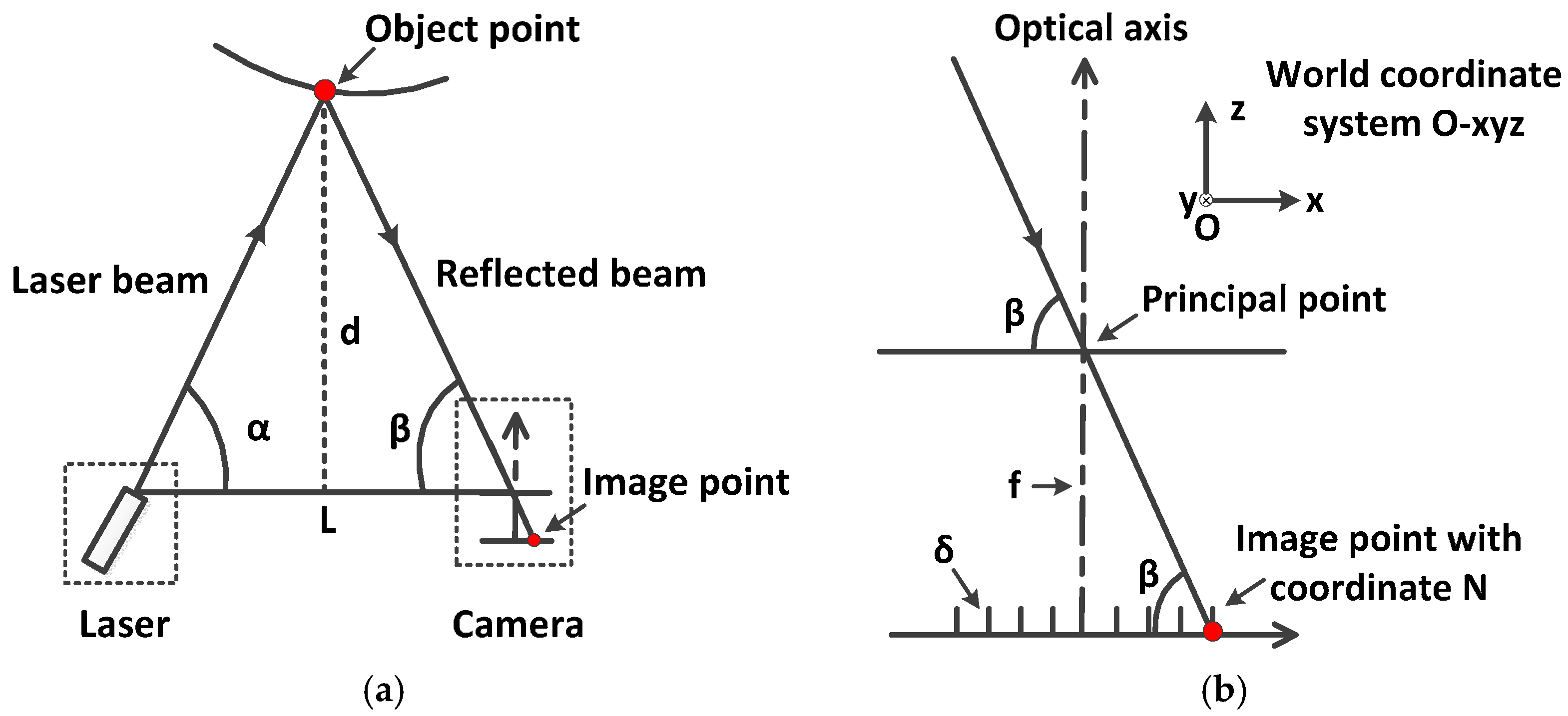
Figure 3.
Simulation result of Formula (3)/Formula (4).

Figure 4.
The coplanar property of the emitted laser beam, the optical axis and the slit. Only when the coplanar property is satisfied, can the laser point pass through the slit and be imaged on the focal plane.
Figure 4.
The coplanar property of the emitted laser beam, the optical axis and the slit. Only when the coplanar property is satisfied, can the laser point pass through the slit and be imaged on the focal plane.
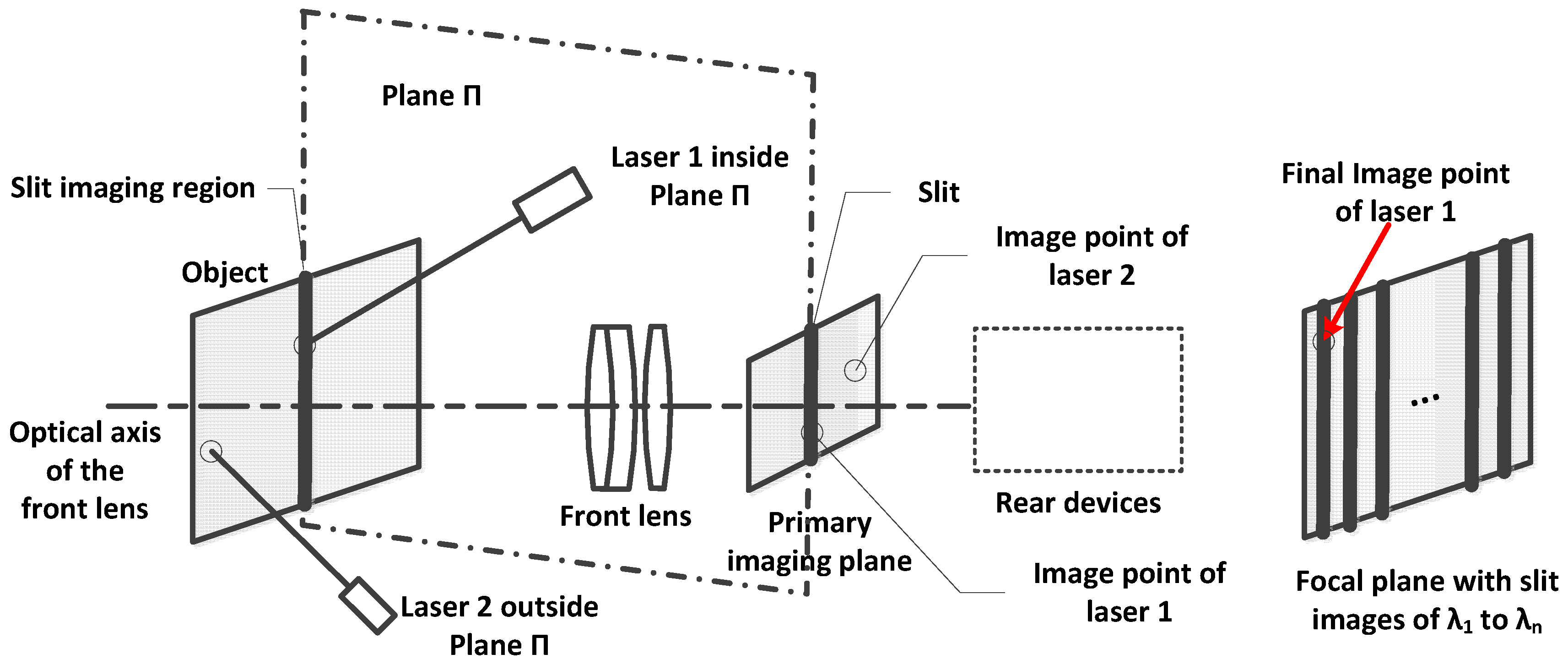
Figure 5.
Schematic of a raw image of the proposed prototype.
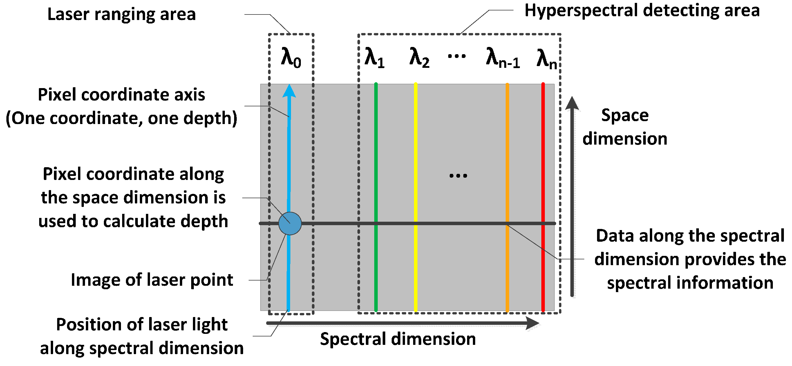
Figure 6.
Schematic map and photo of the prototype. (a) Schematic map; (b) Photo.
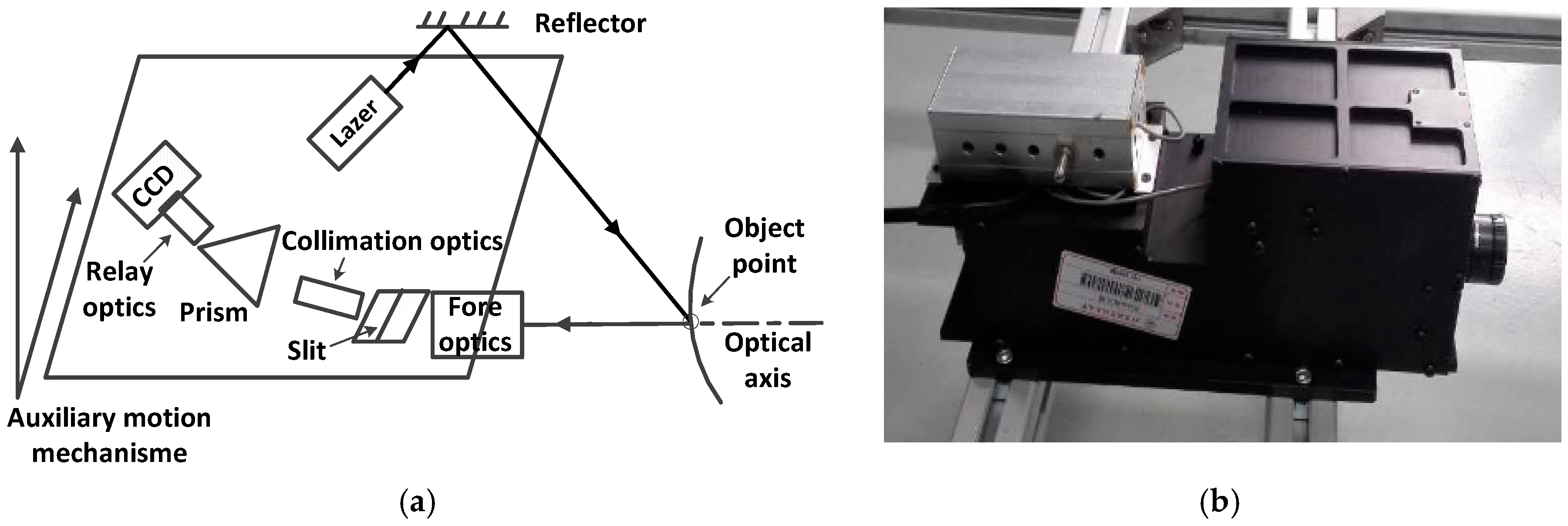
Figure 7.
The spectral measurement with ASD and prototype. (a) Pepper seedling; (b) The prototype; (c) The ASD spectroradiometer; (d) Spectral reflectance; (e) Relative error.
Figure 7.
The spectral measurement with ASD and prototype. (a) Pepper seedling; (b) The prototype; (c) The ASD spectroradiometer; (d) Spectral reflectance; (e) Relative error.
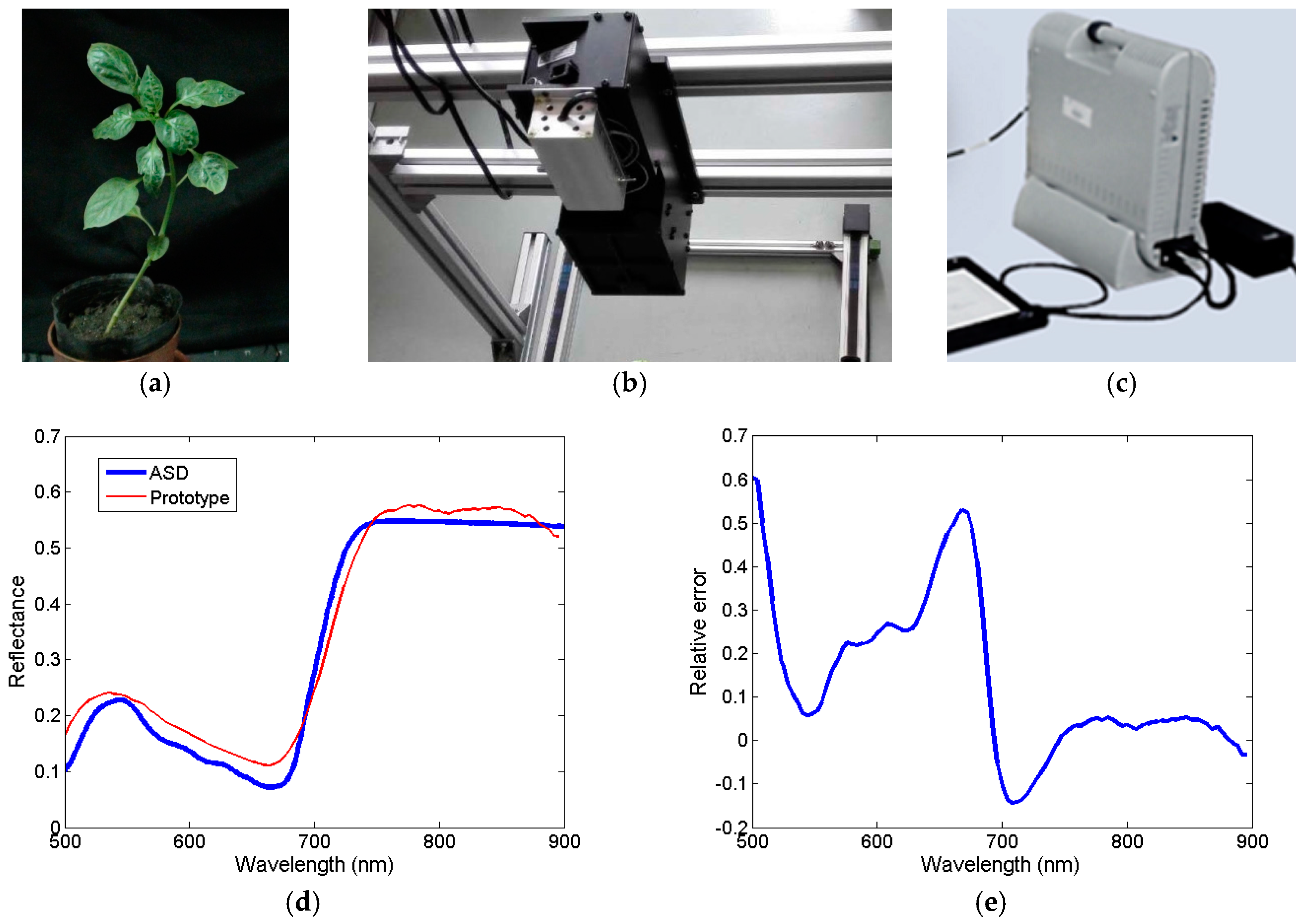
Figure 8.
Spectral experiment of maize seedlings. (a) Photo; (b) Spectral curves of the leaves.

Figure 9.
The standard spheres (a) and the 3D point cloud (b) (with the background points deleted) acquired by the prototype.
Figure 9.
The standard spheres (a) and the 3D point cloud (b) (with the background points deleted) acquired by the prototype.

Figure 10.
The prototype is at a top view of the plant.

Figure 11.
Measuring results of different kinds of vegetation. (a) Maize seedling (with dense 3D points); (b) Tomato seedling (with sparse 3D points); (c) Pepper seedling (with sparse 3D points).
Figure 11.
Measuring results of different kinds of vegetation. (a) Maize seedling (with dense 3D points); (b) Tomato seedling (with sparse 3D points); (c) Pepper seedling (with sparse 3D points).

Table 1.
Parameters of the monochromator.
| Item | Parameters |
|---|---|
| Mode | SP2300 |
| Scan range | 0–1400 nm |
| Wavelenght accuracy | ±0.2 nm |
| Repeatability | ±0.05 nm |
| Minimum drive step size | 0.005 nm |
Table 2.
Parameters of the prototype.
| Slit Width | Spectral Range | Spectral Resolution | Working Distance (WD) | Pixel Size at WD |
|---|---|---|---|---|
| 100 µm | 500–900 nm | 4–8 nm @500–600 nm 8–15 nm @600–900 nm | 150–300 mm | 0.036–0.072 mm |
| Depth Accuracy | X and Y Positioning Accuracy | Laser Wavelength | Laser Point Size at WD | Measuring Speed |
| ±0.5 mm | ±0.03 mm | 450 nm | 0.8–1.2 mm | 10 points/s |
Table 3.
Result of the 3D measurement.
| Parameters | Sphere 1 | Sphere 2 |
|---|---|---|
| Measurement distance | 250 mm | 250 mm |
| Nominal diameter | 22.20 mm | 22.20 mm |
| Measured diameter | 21.87 mm | 21.84 mm |
| Error | −0.33 mm | −0.36 mm |
| Number of measured points | 3532 | 3757 |
| Time consumed | 370 s | 400 s |
© 2017 by the authors. Licensee MDPI, Basel, Switzerland. This article is an open access article distributed under the terms and conditions of the Creative Commons Attribution (CC BY) license (http://creativecommons.org/licenses/by/4.0/).
Share and Cite
MDPI and ACS Style
Zhao, H.; Shi, S.; Gu, X.; Jia, G.; Xu, L. Integrated System for Auto-Registered Hyperspectral and 3D Structure Measurement at the Point Scale. Remote Sens. 2017, 9, 512. https://doi.org/10.3390/rs9060512
AMA Style
Zhao H, Shi S, Gu X, Jia G, Xu L. Integrated System for Auto-Registered Hyperspectral and 3D Structure Measurement at the Point Scale. Remote Sensing. 2017; 9(6):512. https://doi.org/10.3390/rs9060512
Chicago/Turabian StyleZhao, Huijie, Shaoguang Shi, Xingfa Gu, Guorui Jia, and Lunbao Xu. 2017. "Integrated System for Auto-Registered Hyperspectral and 3D Structure Measurement at the Point Scale" Remote Sensing 9, no. 6: 512. https://doi.org/10.3390/rs9060512
Note that from the first issue of 2016, this journal uses article numbers instead of page numbers. See further details here.