
Impacts of Thermal Time on Land Surface Phenology in Urban Areas


1
Geospatial Sciences Center of Excellence, South Dakota State University, Brookings, SD 57007, USA
2
Department of Geography, South Dakota State University, Brookings, SD 57007, USA
3
Department of Natural Resource Management, South Dakota State University, Brookings, SD 57007, USA
*
Author to whom correspondence should be addressed.
†
These authors contributed equally to this work.
Remote Sens. 2017, 9(5), 499; https://doi.org/10.3390/rs9050499
Submission received: 21 February 2017
/
Revised: 3 May 2017
/
Accepted: 13 May 2017
/
Published: 18 May 2017
(This article belongs to the Special Issue Land Surface Phenology and Seasonality: Novel Approaches and Applications)
Abstract
:Urban areas alter local atmospheric conditions by modifying surface albedo and consequently the surface radiation and energy balances, releasing waste heat from anthropogenic uses, and increasing atmospheric aerosols, all of which combine to increase temperatures in cities, especially overnight, compared with surrounding rural areas, resulting in a phenomenon called the “urban heat island” effect. Recent rapid urbanization of the planet has generated calls for remote sensing research related to the impacts of urban areas and urbanization on the natural environment. Spatially extensive, high spatial resolution data products are needed to capture phenological patterns in regions with heterogeneous land cover and external drivers such as cities, which are comprised of a mixture of land cover/land uses and experience microclimatic influences. Here we use the 30 m normalized difference vegetation index (NDVI) product from the Web-Enabled Landsat Data (WELD) project to analyze the impacts of urban areas and their surface heat islands on the seasonal development of the vegetated land surface along an urban–rural gradient for 19 cities located in the Upper Midwest of the United States. We fit NDVI observations from 2003–2012 as a quadratic function of thermal time as accumulated growing degree-days (AGDD) calculated from the Moderate-resolution Imaging Spectroradiometer (MODIS) 1 km land surface temperature product to model decadal land surface phenology metrics at 30 m spatial resolution. In general, duration of growing season (measured in AGDD) in green core areas is equivalent to duration of growing season in urban extent areas, but significantly longer than duration of growing season in areas outside of the urban extent. We found an exponential relationship in the difference of duration of growing season between urban and surrounding rural areas as a function of distance from urban core areas for perennial vegetation, with an average magnitude of 669 AGDD (base 0 °C) and the influence of urban areas extending greater than 11 km from urban core areas. At the regional scale, relative change in duration of growing season does not appear to be significantly related to total area of urban extent, population, or latitude. The distance and magnitude that urban areas exert influence on vegetation in and near cities is relatively uniform.
1. Introduction
Recent increases in population have largely been concentrated in urban areas, increasing from only 13% of total global population in 1900 to 54% by 2014 [1,2]. Urban land expansion has irreversible impacts on the natural environment, including the loss of agricultural lands, fragmentation of ecosystems, reduction of biodiversity, and alteration of local climate [3]. Urban land cover/land use and change can potentially alter local to regional climate on daily, seasonal, and even annual scales [4]. Possibly the clearest example of urban climate modification is the phenomenon where urban temperatures are generally higher than the surrounding countryside, or the urban heat island (UHI) effect [5]. UHI intensity is related to patterns of land use/land cover changes, including the composition of water, vegetation, and built-up areas [6]. The effects of the UHI and land use/land cover change are linked to modified surfaces that affect the transfer and storage of airflow, water, and heat [7].
Future climate change and urbanization is projected to increase UHI temperatures by around 1 °C per decade [8]. The combination of urban population growth, urbanization, and climate change warrants the need for enhanced remote sensing research on the environmental impacts of urban areas and urbanization on the natural environment [9,10]. Specifically, there have been calls for urban remote sensing research of small to medium sized cities and their associated impacts on vegetation [11].
Urban land surface phenology (LSP) observes the spatiotemporal development of the vegetated land surface as revealed by satellite sensors [12] in and nearby cities. The majority of urban LSP studies have used surface observation networks [13] or coarse spatial but high temporal resolution satellite data from sensors including the Advanced Very High Resolution Radiometer (AVHRR) [14] and more recently, the Moderate Resolution Imaging Spectroradiometer (MODIS) [15,16,17]. Jochner et al. [18] provide an overview of observational studies from European, North American, and Asian cities that all found earlier vegetation development in urban areas [18], beginning with a study in Hamburg, Germany in 1955 [19]. Additional studies have used species composition [20] and plant specific phenology [21] in order to characterize the influence of UHIs on vegetation development in cities.
Satellite data based studies that use land surface temperature (LST) data in place of air temperature measurements observe the surface urban heat island (SUHI). One major difference between air temperature studies of UHIs and satellite remote sensing based studies of SUHIs is that SUHI intensity is related to land cover/land use and SUHI intensity is greater during the daytime compared to at night [22]. Studies using coarse resolution satellite data have found that, on average, urban areas expanded the growing season of vegetation by 7.6 days in the eastern United States using time series of the NDVI derived from AVHRR data [14]. Coarse resolution studies have used a combination of LST and Enhanced Vegetation Index (EVI) data time series derived from MODIS to analyze the effects of the UHI on vegetation phenology [15,16]. Important findings from these studies include: (1) the length of growing season for forests is strongly related to mean annual LST [15]; (2) earlier green-up and later dormancy occurs in urban areas [15,16]; and (3) urban climate influences on vegetation phenology extend up to 10 km beyond the urban land cover extent of cities in eastern North America [15]. The UHI effects were found to be stronger in North America than in Asia or Europe [16].
While surface observation networks and high temporal/coarse spatial resolution remote sensing studies are useful, there exists a need for more spatially extensive, higher spatial resolution data products to capture phenological patterns in areas with heterogeneous land cover and external drivers such as urban areas that are a mixture of land cover/land uses and experience microclimatic influences, namely the UHI effect [23,24]. Using Landsat data for phenology studies allows for local to regional scale analyses, offering a spatial resolution that is useful for exploring factors that influence phenology including land use and urban heat islands [24]. One study used Landsat 5 Thematic Mapper (TM) and Landsat 7 Enhanced Thematic Mapper Plus (ETM+) time series to model phenology in eastern United States deciduous forests and found a significant relationship between distance from urban core and green-up onset, suggesting that UHI impacts are reflected in the phenological characteristics of surrounding vegetation [23]. Another study modeled Web-Enabled Landsat Data (WELD) NDVI data as a quadratic function of thermal time derived from MODIS LST data and derived LSP metrics to observe the response of vegetation to UHIs for two cities (Minneapolis-St. Paul, MN and Omaha, NE) in the Upper Midwest region of the United States and found that proximity to the center of both cities was positively associated with increased duration of growing season for perennial vegetation [25]. Even more recently, a study fused MODIS and Landsat reflectance data in addition to LST derived from Landsat thermal data and found that in general, Ogden, UT experienced earlier start of season, later end of season, and consequently longer length of season than the surrounding exurban areas [26].
There are multiple reasons why the Upper Midwest is an ideal location for studying the impacts of urban areas on LSP within and surrounding cities. The region is a relatively flat, continental, temperate plain that is distant from confounding meteorological influences such as major mountain ranges or large water bodies. Cities in the region are relatively isolated and embedded in a vegetated landscape (Figure 1a). The cities span size (area and population) and latitudinal gradients, but precipitation is relatively uniform over the region. The combination of WELD-derived NDVI, MODIS LST-derived accumulated growing degree-days (AGDD), and National Land Cover Database (NLCD) Land Cover Type (LCT) and Impervious Surface Area (ISA) data, all freely available, spanning at least a decade, at a spatial resolution that is appropriate for urban areas, provides an opportunity to investigate the UHI-related impacts on LSP at the local to regional scale at 30 m spatial resolution.
In this study, we analyzed the impacts of urban areas and UHIs on the seasonal development of vegetation on an urban–rural gradient at the local to regional scale for 19 small to medium sized cities located in the Upper Midwest region of the United States. We used satellite remote sensing time series data to investigate the impacts of urban areas on the seasonal development of vegetation using model-derived LSP metrics. We explored the spatial arrangement of urban areas in order to understand the influence of subregions of highly concentrated impervious surfaces and large areas of urban vegetation on microclimatic conditions within cities. We analyzed the distance and magnitude of urban alteration of local atmospheric conditions in and around cities. We compared the results from all 19 cities in order to analyze the influences of city size, land cover, spatial arrangement, and latitude on the seasonal development of vegetation.
2. Materials and Methods
2.1. Study Region
We analyzed remotely sensed vegetation dynamics for 19 cities in the Upper Midwest of the United States. Our region of interest is between 47.5°N, 99°W and 40.5°N, 92°W (Figure 1a,b). An early study of urban climate characterized the nature of UHIs under “ideal” conditions, described as a city situated on flat terrain with population greater than 100,000 and a temperate climate [27]. We chose the Upper Midwest and 19 cities for multiple reasons, including that: (1) there are a number of useful, relatively high resolution (spatial and temporal) remote sensing datasets freely available for the Contiguous United States (CONUS) [28,29,30]; (2) the region is characterized as a temperate plain with relatively isolated urban areas situated within a largely vegetated landscape that experiences distinct annual seasonality; and (3) the cities capture multiple gradients in population size, urban area, land cover type, thermal regime, and latitude. Figure 1b demonstrates the southwest to northeast gradient in annual accumulated growing degree-days, a measure of thermal time that influences the growing season of perennial vegetation.
We selected 19 cities as defined by the United States Census Bureau “Urban Areas” [31] located within the Upper Midwest. These 19 cities span three orders of magnitude in population size, from ~15,000 in Cambridge, MN to 3.4 million in the Minneapolis-St. Paul metropolitan statistical area [32]. The cities also cover three orders of magnitude in terms of urban extent, ranging from ~25 km2 in Brookings, SD to 2773 km2 in Minneapolis-St. Paul, MN in 2010 [33]. Total urban extent for the 19 cities increased by almost 40,000 hectares (18.2%) from 2001 to 2011 [29]. Table 1 provides the information on size, location, and thermal regime for each of the 19 cities included in the analysis. The study time period spans 2001–2012, which covers the 2001, 2006, and 2011 NLCD LCT and ISA archives [29,30], as well as the ten-year (2003–2012) time series available from the CONUS WELD project [28].
2.2. Data
2.2.1. MODIS Land Surface Temperature and Snow Cover Extent
MODIS is a sensor aboard the Aqua and Terra satellites [34]. Aqua and Terra are NASA Earth Science satellites that operate as a part of the Earth Observing System [35]. We used the MODIS-Aqua (MYD11A2) and MODIS-Terra (MOD11A2) products, which are the level-3 global Land Surface Temperature and Emissivity 8-day composites with 1 km resolution, and are provided in Sinusoidal grid format as the mean clear-sky LST values during an 8-day time frame [36]. The specific Scientific Datasets (SDs) extracted from the product included “LST_Day_1km” and “LST_Night_1km” for MODIS tiles h10v04 and h11v04 [36]. We also downloaded the MODIS Aqua (MYD10A2) and Terra (MOD10A2) Snow Cover products, which contain level-3 global “Maximum Snow Extent” 8-day composites at 500 m resolution [37]. Both MODIS products were downloaded for the time period of 2003 to 2012. MODIS 8-day composite products contain 46 annual observations. We used four MODIS 8-day composite products for two MODIS tiles for ten years, resulting in 3680 total MODIS files used in the study.
2.2.2. Web-Enabled Landsat Data
Web-Enabled Landsat Data (WELD) is a NASA-funded project that generated 30 m composited mosaics of the conterminous United States and Alaska using Landsat 7 ETM+ scan line corrector-off data from 2003–2012 [28]. WELD was designed to make consistent Landsat data readily available to develop land cover, biophysical, and geophysical products in order to study Earth system science and regional land-cover dynamics [28]. One advantage of WELD is that the weekly composites include a pre-calculated NDVI band as well as additional quality control flags (saturation, clouds) [28]. We selected all WELD tiles within 40 km of the urban extent (UE) for each of the 19 cities. We filtered out saturated and cloudy observations using the “Saturation_Flag”, “DT_Cloud_State”, and “ACCA_State” bands [28], as well as a filter based on a threshold value of NDVI > 0.2 to exclude non-vegetated observations.
2.2.3. National Land Cover Database
The National Land Cover Database (NLCD) provides 30 m resolution land surface characteristics over the United States that can be used for applications including assessment of ecosystem health and ecosystem status [38]. We used the Percent Developed Imperviousness [29] and Land Cover Type [30] products from 2001, 2006, and 2011. The Impervious Surface Area product was determined using IKONOS and Landsat 7 ETM+ data and estimated the percentage of each 30 m pixel covered by anthropogenic (concrete, asphalt, etc.) surfaces [39]. The Land Cover Type product was derived from unsupervised classification of Landsat 5 TM and Landsat 7 ETM+ at a spatial resolution of 30 m [30]. The datasets are freely available for download from the Multi-Resolution Land Characteristics Consortium website [29,30].
2.3. Methods
2.3.1. Spatial Arrangement of Urban Areas
We defined the region of interest for each city as the area within 40 km of the urban extent for each of the 19 cities. We characterized the region of interest for each city based on the 2001, 2006, and 2011 LCT and ISA datasets by identifying the LCT and ISA for each corresponding 30 m WELD pixel located in each region. We used a decision tree classification scheme to aggregate the 16-class LCT data into nine classes. Table 2 shows the class groupings used. We also performed change detection from 2001 to and from 2006 to 2011 to identify pixels that experienced a change in LCT, ISA, or both and classified pixels with ISA change into two classifications based on time period: (1) “2001–2006” change; and (2) “2006–2011” change (Table 2). Pixels classified as “Water”, “Barren”, “2001–2006 Change” and “2006–2011 Change” were excluded from the analysis. Figure 2a illustrates the LCT classification over Sioux Falls, SD.
In order to characterize the spatial arrangement of heterogeneous urban landscapes, we defined four specific urban spatial subregions of interest. We used the 2010 U. S. Census Bureau delineated “urban areas” cartographic boundary shape files to define Urban Extent (UE) for each urban area [33]. We identified Urban Core Area (UCA), which we defined as a spatially contiguous area of pixels (>10 hectares) located within the UE of each city and classified as “Developed, High Intensity” based on the 2011 LCT dataset. Green Core Area (GCA) is defined as a spatially contiguous area of pixels (>60 hectares) located within the UE of each city and classified as “Developed, Open Space”, “Forest”, “Shrub/Scrub”, “Grassland/Herbaceous”, “Pasture/Hay”, or “Wetlands” based on the 2011 LCT dataset. The UCA and GCA size thresholds were determined so that each city contained at least one of each urban spatial subregion. Pixels located outside of the UE but within the 40 km region of interest are simply classified as “Outside of the Urban Extent”.
After identifying the boundaries for: (1) UE; (2) UCAs; (3) GCAs; and (4) areas outside of the UE, we calculated Euclidean distance from each pixel to the nearest UCA. Distance is rounded to the nearest kilometer. To control for the compounding factor of nearby cities influencing vegetation, Each individual cities’ 40 km region of interest was reconfigured after Euclidean distance calculation to group pixels by distance to nearest UCA by city, rather than simply the nearest urban extent. This means that while a pixel may be closer to the boundary of one city, it may actually be closer to the core area of a different city.
2.3.2. Thermal Time
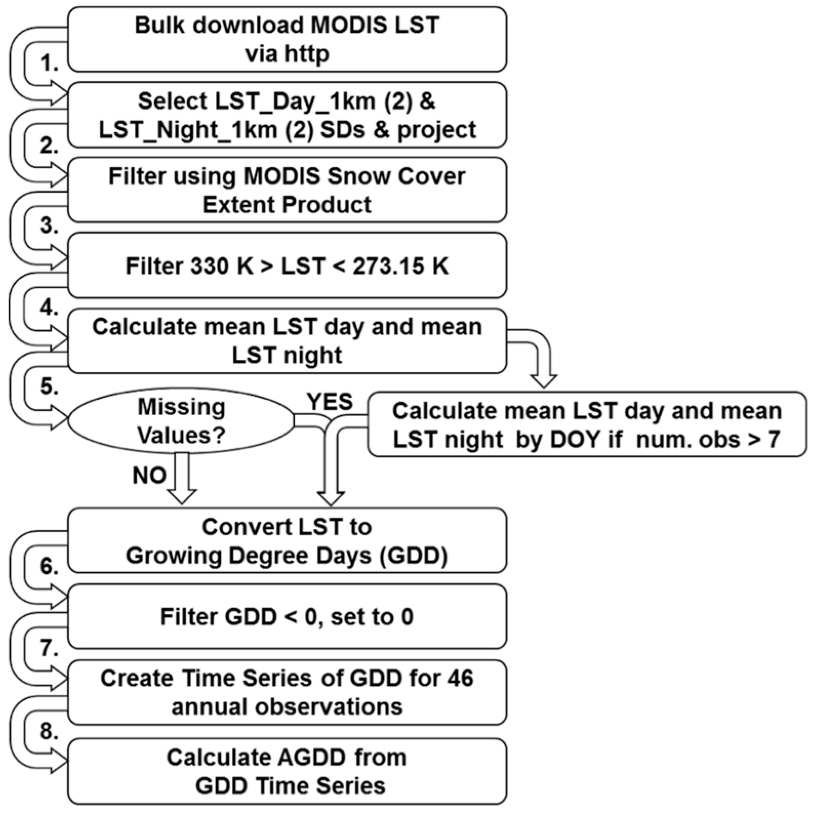
We used the maximum snow extent product to exclude MODIS LST observations when snow cover was present. The MODIS LST observations were additionally filtered to exclude observations that were below freezing (273.15 K), or unreasonably high (330 K). We revised an algorithm developed in [40] that converts the two daytime and two nighttime LST observations into growing degree-days (GDD), and ultimately into an annual accumulated growing degree-day (AGDD) product. The algorithm was used to calculate a climatology of thermal time, the average daytime and nighttime LST for each day of year (DOY) (using the ten years available for each date), which was later used to fill gaps arising from missing or excluded data. However, the mean LST by DOY is only calculated when eight or more years have available data. The algorithm also calculated GDD. The traditional calculation of GDD takes the mean of the daily maximum and minimum temperature and subtracts a base temperature threshold. The GDD calculation used the mean of the mean daily and mean nightly LST values and a base of 0 °C:
When GDD < 0, the daily value was mapped to zero, meaning no increment of thermal time occurred during that compositing period. Then the annual time series of GDD composites was multiplied by 8 to account for the 8-day compositing period of the MODIS products and accumulated each observation (GDD in °C) across the year. The final product is a ten-year time series of accumulated growing degree-days (AGDD in °C) by year. Figure 3 shows the workflow for the MODIS LST to AGDD conversion process.
2.3.3. Land Surface Phenology Modeling
LSP metrics are often calculated from time series data of vegetation indices [41]. There are four main methods used to calculate LSP metrics, including: (1) thresholds; (2) derivatives; (3) smoothing functions; and (4) fitting models [41]. We used a quadratic regression model to link the WELD normalized difference vegetation index (NDVI) to MODIS LST-derived AGDD. This model has been used successfully to analyze LSP dynamics in temperate regions [12,17]. The quadratic LSP (Q LSP) model is defined as:
where NDVI contains all NDVI values (unitless; −1 to 1) for a specific period and AGDD (°C) contains all AGDD values for the corresponding period [42]. The Q LSP model requires only three model parameter coefficient estimates with relevant ecological interpretations [42,43]. The significance of the model is dictated by its ability to explain the variance in NDVI, expressed as the coefficient of determination (R2). We applied the Q LSP model to the decadal time series of NDVI and AGDD observations for each pixel and derived the following LSP metrics:
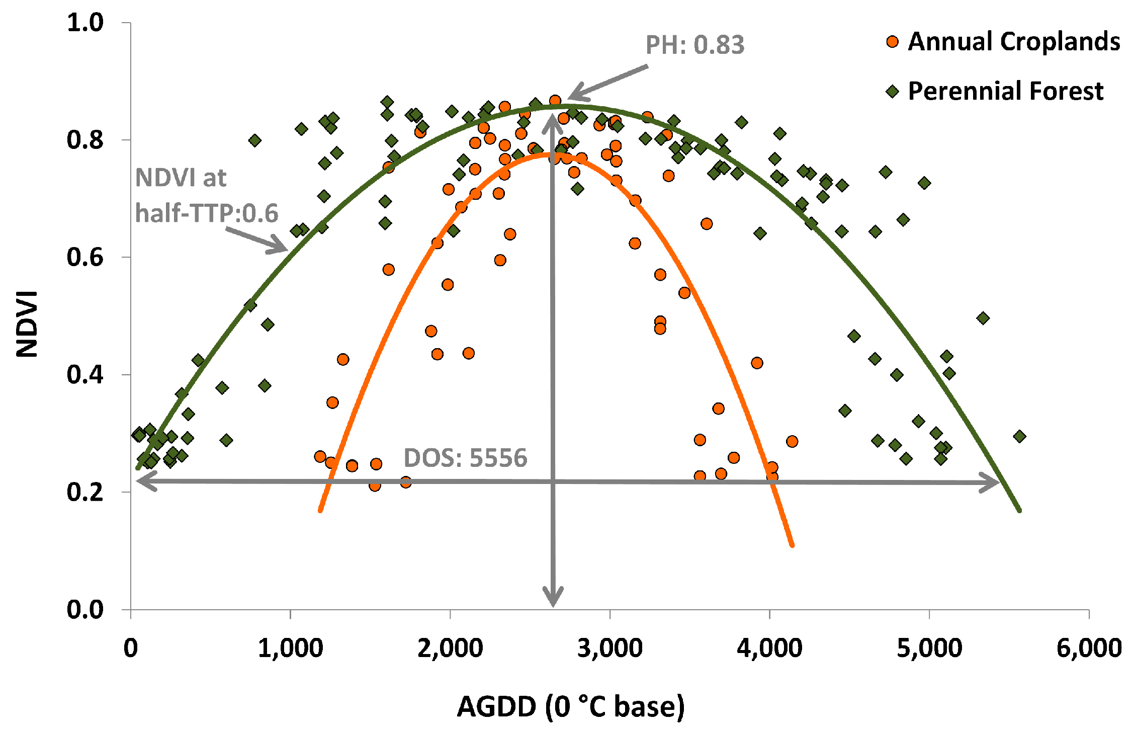
We derived NDVI at half-thermal time to peak (half-TTPNDVI) from PHNDVI and TTP. We used a threshold of NDVI = 0.3 to determine Start of Season (SOS) and End of Season (EOS) for a given pixel. This threshold was chosen because all NDVI values are filtered to select observations where NDVI > 0.2, and thus once NDVI = 0.3, vegetation has increased in NDVI. NDVI is then input and solved for in Equation (2) for both sides of the quadratic parabola (i.e., SOS and EOS). This provides AGDD at SOS and EOS, from which the difference of (EOS-SOS) determines the Duration of Growing Season (DGSAGDD). We used a coefficient of determination threshold of R2 < 0.5 to exclude ill-fitting models. Figure 4 demonstrates the fitting of the Q LSP model to a decade of NDVI vs. AGDD observations and the associated LSP metrics derived from the model.
2.3.4. Equivalence Testing
In order to determine if significant differences exist in DGSAGDD between GCAs, UE areas, and areas outside of the UE, we performed a statistical analysis known as equivalence testing. We used the two one-sided tests (TOST) approach to test for equivalence between group means [44]. Tests of equivalence evaluate the similarity between two groups rather than the more commonly used tests of difference or inequality [45]. There are multiple reasons why equivalence tests are more appropriate for our study than more traditional tests of significant differences between two groups. First, when sample size n is extremely large (~10 M pixels in the Minneapolis-St. Paul region), difference tests may prove statistically significant for any non-zero difference in group means [45,46]. Moreover, remote sensing data suffer from high positive spatial autocorrelation and it is difficult to correct for positive spatial autocorrelation in difference testing [47]. Another benefit of equivalence testing is that it allows for interpretation of the magnitude of differences between two groups [45,48]. Contrary to tests of difference, the null hypothesis in an equivalence test is that two groups are significantly different [45]. In order to test for equivalency, a zone of indifference is specified which identifies the upper and lower bounds to test for a difference in means between two groups.
We performed equivalence tests on the difference between group means of LSP metrics for GCAs, UE areas, and areas outside of the UE, adjusting for multiple comparisons using the Bonferroni correction method [49]. The LSP metrics tested include TTP and DGSAGDD. To objectively determine the zone of indifference, or δ, we used 10% of the mean for each LSP metric for each of the 19 study cities. When testing for equivalence between group means of LSP metrics between GCAs, UE areas, and areas outside of the UE, four conditions were possible: (1) all three groups to be statistically equivalent; (2) all groups to be different; (3) one pair of group means to be equivalent, and two pairs different; or (4) two pairs of group means equivalent, and one pair different. In the analysis, the letters were ranked in descending order; same letters indicate the groups were equivalent.
2.3.5. Exponential Trend Model
A study on urban climates in 70 cities in eastern North America found the ecological footprint of cities to be 2.4 times greater than the extent of urban land use, which was determined as the distance where 95% of asymptotic values were reached in the exponential model of differences in green-up onset and dormancy onset as a function of distance from the urban perimeter [15]. Here we used a similar method to calculate the difference in duration of growing season between urban and surrounding rural areas and to determine the magnitude and extent of urban influence on the seasonal development of vegetation.
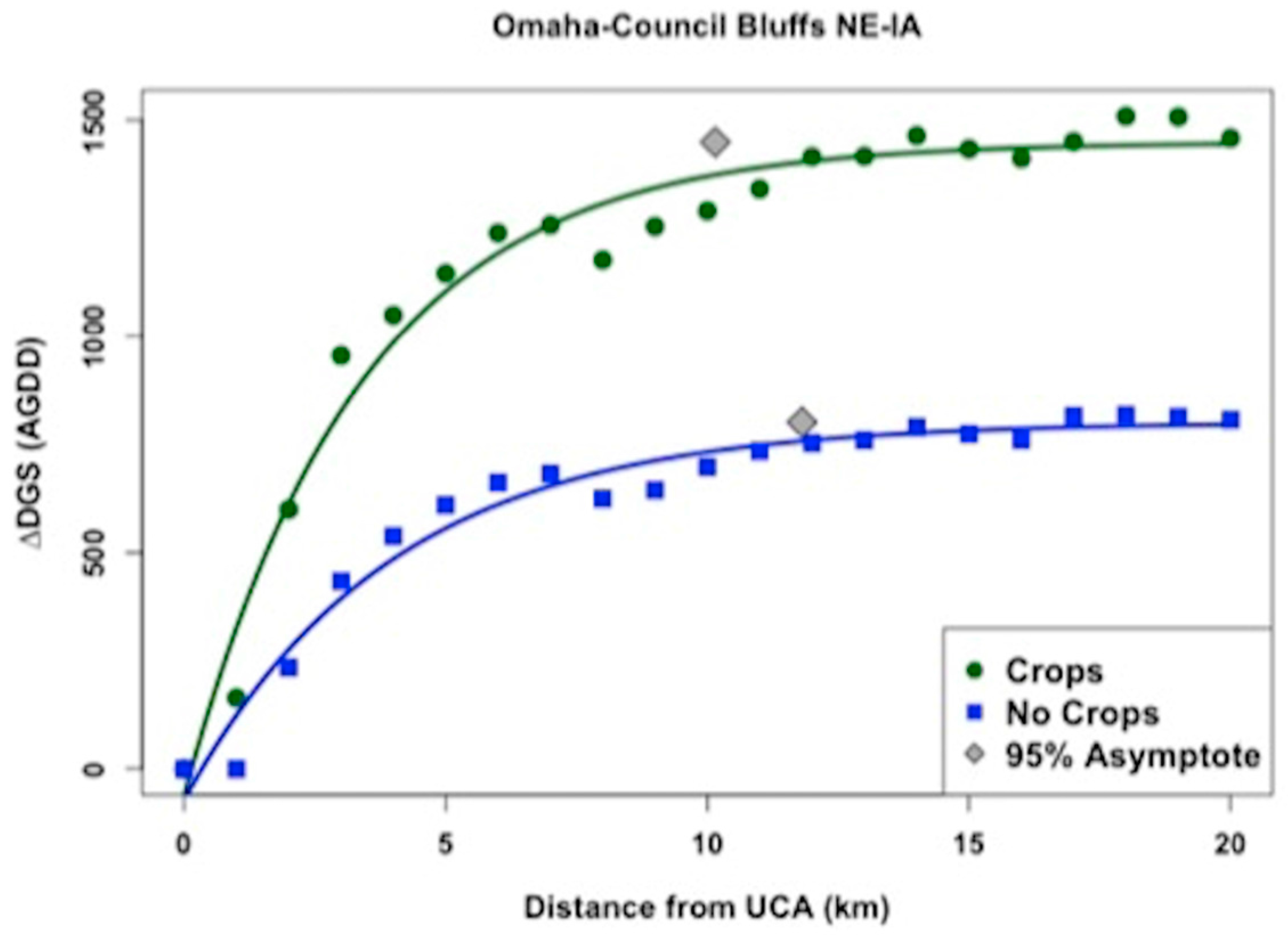
We calculated the mean DGSAGDD for all pixels with R2 > 0.6 within each cities’ UE. Next, we calculated the mean DGSAGDD grouped by distance from nearest UCA at 1 km intervals, and took the difference between mean UE DGSAGDD and the mean DGSAGDD for each 1 km distance grouping. We plotted the mean difference in DGSAGDD (ΔDGSAGDD) as a function of distance from UCA for each city (Figure 5). From there, we fitted an exponential function (Equation (5)), where a is the horizontal asymptote, u is the relative amount the curve increases from the origin to the horizontal asymptote, and b is a scaling parameter for distance.
We assumed that the distance from UCAs where impacts on DGSAGDD become insignificant is the distance where each exponential model reaches 95% of its asymptotic values [15]. This approach provided two values: (1) the extent (distance) of urban influence on LSP; and (2) the magnitude of differences in DGSAGDD between urban and surrounding rural environments.
We limited this analysis to all pixels within 20 km of UCAs, the same distance used in [15]. The analysis was split into two parts. The first was limited to perennial vegetation LCTs, whose DGSAGDD is driven largely by local atmospheric conditions and thus allows for conclusions to be made on the impacts of UHIs on DGSAGDD. Second, we performed the same analysis but included annual croplands. It would be inappropriate to draw conclusions on the influence of urban areas (via the UHI effect) on the DGSAGDD of croplands, because cropland LSP is driven largely by management practices, including the timing of tillage and harvest [25]. However, including croplands allowed us to draw conclusions on the difference in the duration of the “green-on” season. That is, the annual time period when the land surface is covered in green vegetation. At the regional level, we compared results from each urban region to draw conclusions on the influence of city size and latitude in regards to the impacts on the surrounding environment.
3. Results
3.1. Equivalence Testing
Duration of Growing Season
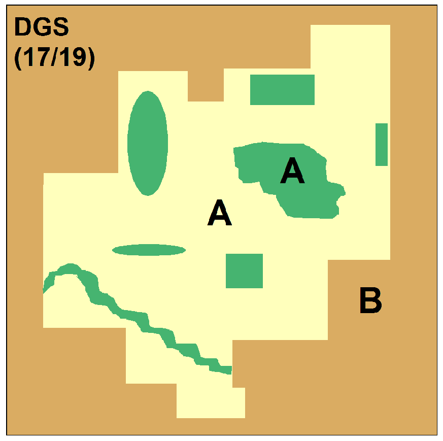
We expected to find that DGSAGDD in GCAs was shorter than in UE areas, but longer than in areas outside of the UE, based on the premise that vast expanses of urban vegetation could potentially experience shorter growing seasons due to the cooling effects of vegetation. However, only one out of the 19 cities exhibits this pattern based on the equivalence testing analysis (Lincoln, NE). We found that DGSAGDD was equivalent between GCAs and UE areas and higher than areas outside of the UE for 17 out of the 19 cities (Figure 6). We concluded that, in general, DGSAGDD was longer in both GCAs and UE areas than in areas outside of the UE, but there was not a significant difference between DGSAGDD in GCAs compared to UE areas. This dominant spatial pattern demonstrated the influence of urban areas and UHIs on the seasonal development of perennial vegetation, where vegetation within cities experienced growing seasons that were at least 10% longer than vegetation in the surrounding rural areas.
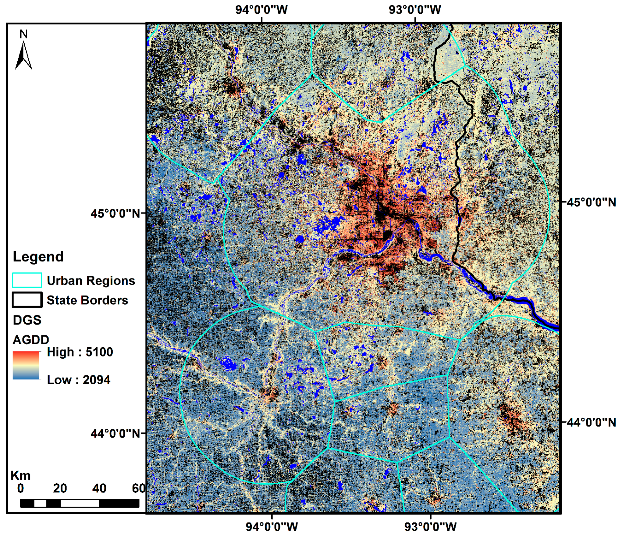
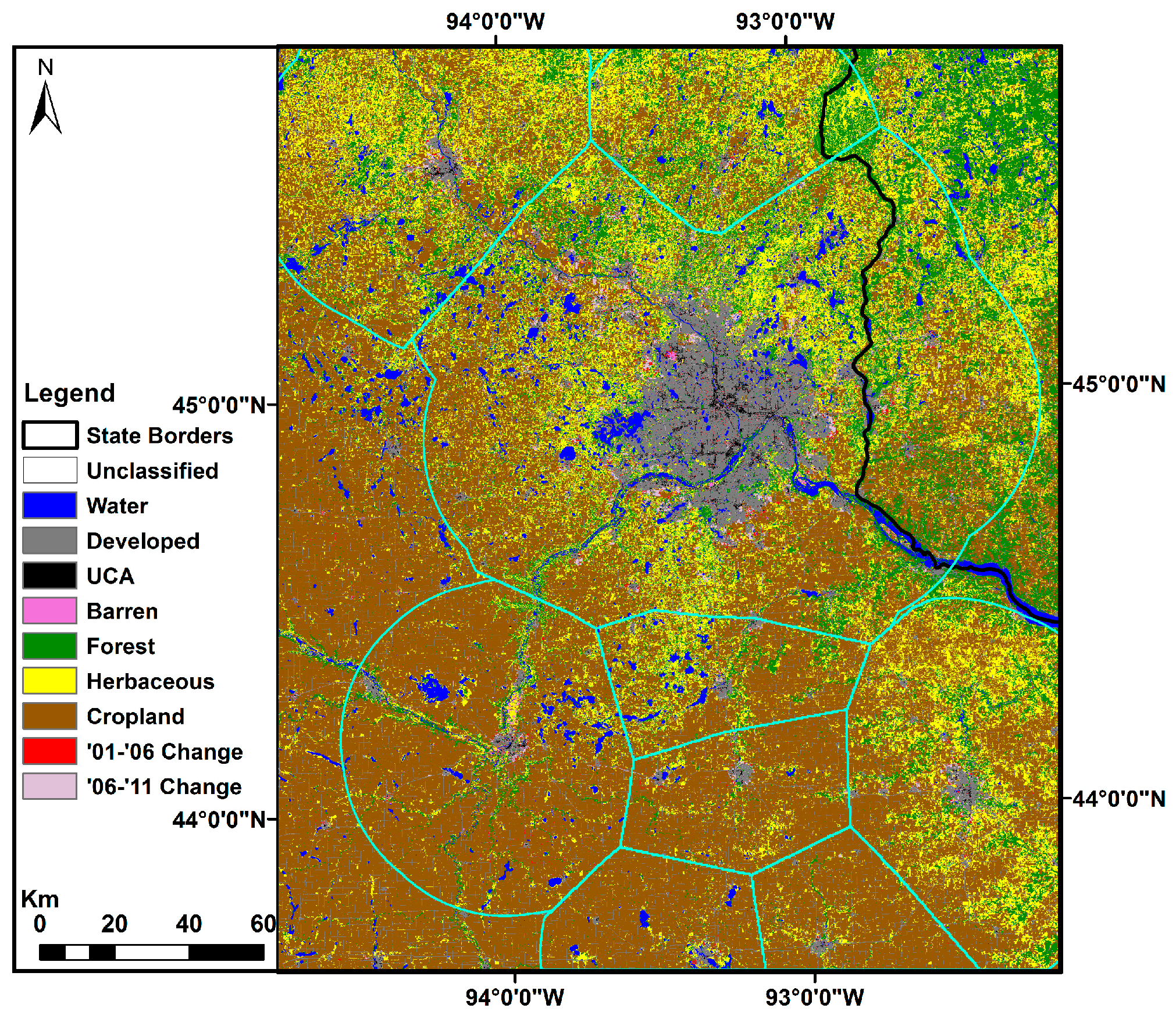
Figure 7 shows DGSAGDD over the Minneapolis-St. Paul, MN region. Darker shades of red relate to longer DGSAGDD, clustered near the densely impervious UCAs of each city. Figure 8 shows the corresponding LCT over the greater Minneapolis-St. Paul region. Notice the higher DGSAGDD in the perennial LCTs (developed, forest, herbaceous) located within the cities compared to annual croplands outside of the urban areas. This spatial pattern demonstrates why croplands were omitted from the DGSAGDD analysis: (1) there are little to no cropland areas inside of cities from which to compare; and (2) the seasonal development of annual croplands is dictated by management factors (i.e., field accessibility, timing of tillage, and irrigation) rather than by local environmental and atmospheric conditions (i.e., thermal time and the UHI effect).
3.2. Exponential Trend Model
To test whether DGSAGDD decreased with distance from UCAs, we analyzed the difference in DGSAGDD between UE areas and areas grouped by increasing distance from UCAs. ΔDGSAGDD followed an increasing negative exponential trend function of distance from UCAs for all of the 19 study cities. However, the Fargo, ND, region exhibited unreasonable results, likely due to the low R2 in the study region (28.6% Q LSP model fit). Thus, we excluded the Fargo, ND, region from the exponential trend model analysis. We fitted the exponential model twice: once for ΔDGSAGDD calculated only from perennial LCTs (developed, forest, and herbaceous) (Figure 9; blue) and once incorporating croplands (Figure 9; green). In general, ΔDGSAGDD increases exponentially with distance from nearest UCA (Figure 9). The magnitude of ΔDGSAGDD ranges from 393 AGDD in Mankato, MN, to 855 in Lincoln, NE. The distance at which urban effects are detectable and significant extends from 5.6 km in St. Cloud, MN, to 15.4 km in Des Moines, IA. The results for each individual city are found in Table 3. On average, the 18 urban areas experience growing seasons that are 669 AGDD longer than the surrounding rural areas, and the effects of urban areas on the growing season extend 11.4 km into the urban periphery. It is evident that urban areas impact the duration of growing season in perennial LCTs, and that urban effects (namely UHIs) extend beyond the boundaries of cities themselves.
Analysis of DGSAGDD restricted to perennial vegetation LCTs allowed for conclusions on the impacts of UHIs on the seasonal development of vegetation. However, including croplands offered a comparison of the difference between urban and rural duration of green-on season, or the annual period where the land surface is covered in green vegetation. Figure 9 demonstrates the dramatic difference in ΔDGSAGDD calculated with (green) and without (blue) annual croplands. Notice that the difference in ΔDGSAGDD was greater in cities that are surrounded predominantly by intensive agriculture (Figure 9; Omaha, NE, and Des Moines, IA) compared to areas where there was a greater portion of forest and herbaceous land cover surrounding the city (Figure 9; Rochester and Minneapolis-St. Paul, MN). Including croplands into the calculation of ΔDGSAGDD led to a mean difference between urban and rural DGSAGDD of 1125 AGDD. To reiterate, this result is not demonstrating the influence of urban areas on local atmospheric conditions, but rather highlights the large difference in the duration of green-on season between perennial vegetation LCTs and annual croplands. This difference has major implications for the representation of urban versus rural vegetation in land surface modeling.
3.3. Regional Comparison
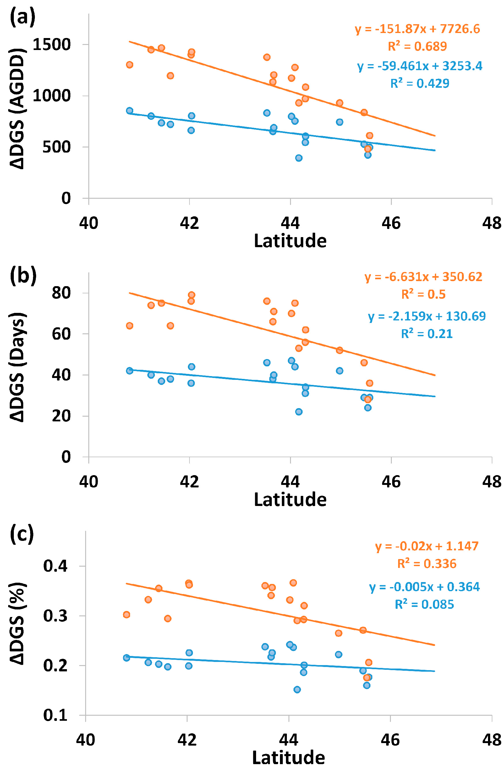
The impacts of urban areas and UHIs on the seasonal development of vegetation were independent of population size. However, the total area influenced by urban areas was larger in cities with greater total area. Figure 10 shows the relationship between latitude and ΔDGSAGDD. In orange are ΔDGSAGDD for each city calculated with croplands, and in blue are ΔDGSAGDD calculated without croplands. It appears that ΔDGSAGDD decreased with increasing latitude in Figure 10a; however, if we converted ΔDGSAGDD into ΔDGSdays (by dividing ΔDGSAGDD by the average daily GDD for each city) the relationship appeared less significant (Figure 10b). If we normalized ΔDGSAGDD as a percentage of the total mean DGSAGDD by city, the relationship appeared even less significant (Figure 10c), and the slope was not significantly different from zero for ΔDGSAGDD with croplands excluded (Figure 10c, blue). The trend in the relationship between ΔDGSAGDD as a function of latitude for the analysis including croplands is likely demonstrating the greater presence of agriculture in the cities located farther south than in the more heavily forested and herbaceous regions surrounding the northern cities (Figure 1a). This pattern suggests that urban influence on local atmospheric conditions is relatively uniform and proportionally not influenced by latitude in our study region. Stated in another way, the exponential trends in ΔDGSAGDD found in this study were not caused by differences in latitude, but rather by urban areas and their associated UHIs.
Based on the results from the equivalence tests between DGSAGDD in urban areas and surrounding rural regions, and the aforementioned differences in DGSAGDD found with increasing distance from urban core areas, we concluded that duration of growing season for perennial vegetation LCTs decreases with distance from urban core areas. We found growing season length to differ by as much as one month between urban areas and their surrounding rural regions. We found the effects of urban alteration of local atmospheric conditions to extend around 11 km from UCAs.
4. Discussion
We had expected to find that the duration of growing season in green core areas would be shorter than in urban extent areas, but longer than areas outside of the urban extent. Duration of growing season was significantly longer in urban extent areas compared to areas outside of the urban extent for all of the 19 cities analyzed. However, duration of growing season was not significantly longer in urban extent areas compared to green core areas, as anticipated. We posited that duration of growing season would be lower in green core areas due to the cooling effects of green vegetation. For example, one study reported that urban parks help control urban temperatures due to 300% higher evaporation rates than the surrounding urbanized area [50]. Another study found that green areas and parks reduce cooling load by 10% [51]. An experiment found that a 600 m2 park was able to decrease temperatures by 1.5 °C [52]. However, one limitation of this study was the relatively coarse spatial resolution (1,000,000 m2) of the MODIS LST product that was used to calculate the accumulated growing degree-days. Although this study did not find significant differences between duration of growing season in green core areas versus urban extent areas, Figure 7 demonstrates that duration of growing season is not spatially uniform throughout cities. It is evident that duration of growing season was longer near urban core areas than in other subregions of the city. Future studies should explore other strategies for subdividing cities into spatial subregions, perhaps using Local Climate Zones (LCZs) [53] as outlined by the recently launched World Urban Database and Portal Tool project [54].
The finding that both green core areas and urban extent areas had significantly higher duration of growing season than areas outside of the urban extent can be attributed to urban areas modulating local atmospheric conditions, namely via increased temperatures and consequently longer growing seasons as a result of the UHI effect. However, there are other factors that may also have contributed to the difference in duration of growing season between urban and rural areas, including decreased wind speed, increased water availability as a result of urban irrigation, and differences in urban–rural species composition. However, the finding that maximum NDVI was significantly lower in urban areas than surrounding rural areas suggests that water availability was likely not the main limiting factor in the Upper Midwest, a region that experiences relatively stable precipitation patterns and quantities, although it is also susceptible to dry extremes [55]. If urban irrigation were the main factor contributing to increased duration of growing season, then we would expect maximum NDVI to be lower in areas outside of the urban extent, which was not found in this study.
The analysis of ΔDGSAGDD demonstrated that urban areas and UHIs influenced the local thermal conditions inside of cities and extended into the urban periphery. On average, this study found that UHIs lengthened the growing season by >600 AGDD and the effects extended around 11 km from the highly impervious, densely urbanized urban core areas. This finding has major implications for land surface phenology in urban to peri-urban environments. To illustrate: if we say that an average growing season day accumulates 20 growing degree-days, and then divide 600 AGDD by 20, this equates to a difference in the duration of growing season by approximately one month between urban areas and surrounding rural areas that are not significantly influenced by local urban atmospheric modification (mainly UHI effects). A previous study found that LST is significantly higher than corresponding air temperatures during the daytime, although similar temperatures were found between LST and corresponding air temperatures at night [40]. Future studies should explore the use of nighttime LST alone in order to exploit the benefits of spatially exhaustive temperature readings that closely correspond with air temperatures in order to remove the bias of higher daytime LST temperatures observed over cities.
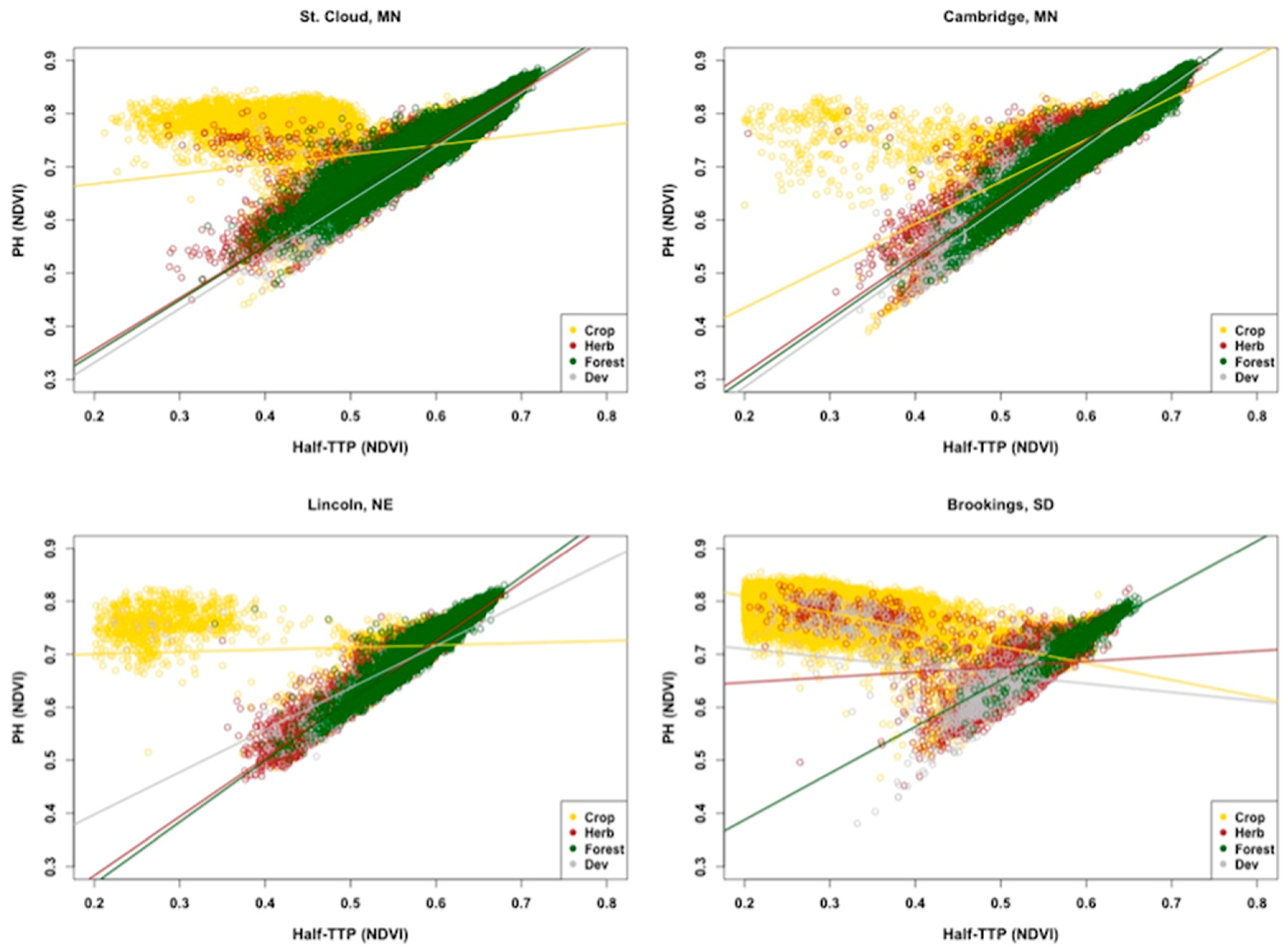
Note that these results are from the analysis of only perennial vegetation land covers (developed, forest, and herbaceous). Perennial vegetation land cover types in this study exhibited a linear trend between peak height in NDVI and NDVI at half-thermal time to peak, suggesting that the seasonal development of perennial vegetation was driven by local atmospheric conditions, namely thermal time. This observation aligns with plant development theory, or the idea that higher temperatures prompt earlier growth in heat-sensitive species [56]. Controlling the analysis to perennial vegetation land cover types provided a higher level of confidence that the results were indeed due to the influence of UHI effects rather than differences in land cover type, specifically between annual croplands and perennial vegetation.
To illustrate the linear trend between peak height in NDVI and NDVI at half-thermal time to peak, we performed linear regression analyses on the relationship between PHNDVI and half-TTPNDVI by land cover type. Due to the high volume of observations, we limited this portion of the analysis to pixels with R2 ≥ 0.8. In order to determine if the linear model (fit to all pixels with R2 ≥ 0.8 from the Q LSP model) was significant, we also used an R2 threshold of 0.8 in addition to the more traditionally used p-values, again due to extremely large n values. We then compared the observed differences between various LCTs. In particular, we were interested in whether a significant linear relationship existed for perennial vegetation LCTs but not for annual croplands. Figure 11 shows an example of the linear relationship between PHNDVI and half-TTPNDVI for perennial vegetation in four of the selected cities.
Incorporating croplands is, however, useful because it demonstrates the differences in green-on season between urban and rural areas, or the time period of the year where the land surface is covered in green vegetation. The addition of annual croplands into the calculation of change in duration of growing season increased the mean difference between urban and rural duration of growing season to around 1100 AGDD, that translates into about two months difference in the period when the land surface has green vegetation. At first, this may sound like an erroneous result; however, the major crops grown in the Upper Midwest, namely maize and soybean, do not begin to develop as soon as the growing season has commenced for perennial vegetation. Rather, the seasonal development of commodity crops, such as maize and soybean, is driven largely by external, non-atmospheric factors including crop management, field accessibility, timing of planting and harvest, or the use of irrigation. This phenomenon is confirmed by the high variation in the rate of vegetation green-up illustrated in cropland pixels in Figure 11. It is not unusual for maize and soybean fields in the Upper Midwest to be mostly bare soil in April–May and either dried-out crops or crop harvest residue in September–October. Meanwhile, perennial vegetation generally begins developing shortly after snow melt and ends after the first hard freeze; these times are undoubtedly much earlier and later, respectively, than the duration of green-on season for maize, soybean, and other summer crops.
The major difference in duration of green-on season between perennial vegetation and annual croplands has major implications for urban–rural differences in heat storage and release during different periods of the year. During the summer months when the crop canopy is fully developed, green vegetation redistributes energy absorbed during the day through evapotranspiration, leading to cooler temperatures in the rural regions surrounding cities [57]. At the regional scale, relative change in duration of growing season does not appear to be significantly related to urban extent, population, or latitude. This finding suggests that the distance and magnitude that urban areas influence vegetation in and near cities is relatively uniform independent of city size. However, larger urban areas have a greater impact on local atmospheric conditions in terms of area.
The positive linear relationship found in the rate of vegetation green-up versus the maximum NDVI in land cover types with perennial vegetation and the high variation in the rate of green-up for annual croplands suggests that studies of UHI impacts on urban land surface phenology need to account for differences in urban/rural land cover types. Because annual cropland phenology is driven largely by agricultural planting schedules, it is not appropriate to use annual cropland land surface phenology metrics in order to draw conclusions on the magnitude and extent of urban heat island effects on land surface phenology in and around cities. Vegetation cover/types that exhibit a perennial vegetation response, i.e., a positive linear relationship between Half-TTPNDVI and maximum NDVI, are more appropriate for research aimed at measuring and monitoring the urban heat island effects on land surface phenology.
5. Conclusions
There are multiple remote sensing issues that must be considered in order to draw conclusions related to the study of UHI impacts on LSP in and around cities. Past studies of UHI effects on urban LSP have centered on surface observation networks and high temporal/coarse spatial resolution remote sensing datasets. Studies of UHIs using air temperature readings from local meteorological stations have higher spatial resolution, but are limited by sparse spatial coverage. Moreover, a recent study on the thermal environment of grasses found that the plants respond more closely to the land surface temperature than to air temperature at two meters [58]. Studies of UHIs using coarse spatial resolution data for analyzing urban LSP suffer from the mixed pixel problem that make it extremely difficult to account for differences in LSP as a function of LCT. There exists a need for more spatially extensive, higher spatial resolution data products to capture phenological patterns in areas with heterogeneous land cover and external drivers, because urban areas are a mixture of land cover/land uses and exhibit microclimatic variation [23,24,25]. Using Landsat data for phenological studies allows for local to regional scale analyses, offering a spatial resolution that is useful for exploring factors that influence phenology including land use and urban heat islands [23,24,25,59].
As a caveat, it is difficult to draw conclusions on maximum NDVI in cities due to the heterogeneous nature of the urban land surface; pixels that are a mixture of an urban lawn and a rooftop, for example, will exhibit lower maximum NDVI values due to the proportion of impervious surface being sensed. Another caveat is that we focused on the surface UHI and thus used AGDD derived from land surface rather than air temperature data.
This regional study leverages multiple datasets from multiple sensors at relatively high spatial resolutions in order to resolve the tradeoff between high spatial and temporal resolution, enabling research to be conducted while controlling for LCT and enabling full spatial coverage in and around cities. Fitting the Q LSP model to a decade of available observations provides a strategy for dealing with the low number of observations that often restrict Landsat studies. This research provides a framework for studying the impacts of urban areas and UHIs on the seasonal development of vegetation at a spatial resolution that is useful and necessary in highly complex, heterogeneous urban areas. The results found in this study highlight the need for future research of UHI-related impacts on urban LSP in order to account for differences in LSP between annual croplands and perennial vegetation covers. In addition, DGSAGDD was found to increase with proximity to densely impervious, urban core areas, demonstrating the need to identify local “hotspots” within urban areas that may disproportionately produce warmer atmospheric conditions. These results that demonstrate the drastic difference in the DGSAGDD and the extent of urban influence on DGSAGDD highlights the need for urban land surface models to accurately represent the seasonal development of vegetation in and nearby cities. Future urbanization will only increase the amount of Earth’s land surface that is significantly impacted by urban areas and associated UHI effects. Future studies will model LSP metrics before and after land cover changes as urbanization occurs along the urban periphery. This step should reduce the number of pixels within cities that were excluded from the analysis due to poor Q LSP model fit, and increase our understanding of the impacts of urbanization on LSP.
This study provides much needed and currently lacking information on: (1) the differences in the seasonal development of vegetation between urban and rural areas of the Upper Midwest of the United States; (2) the magnitude and extent of UHI effects on the seasonal development of vegetation in small to medium sized cities; and (3) the differences in land surface phenology between annual croplands and perennial urban vegetation. More importantly, this study provides a framework for alleviating the resolution problems that have restricted studies of UHI effects on urban LSP in the past. This information should prove useful to inform a variety of interests, including scientists interested in urban thermal climate analyses, as well as urban climate modelers, urban ecologists, urban and regional planners policy-makers, meteorologists, and climatologists.
Acknowledgments
Funds were available to support research and its publication in part by the NASA grants NNX12AM89G and NNX14AJ32G to G.M.H. and cooperative agreement NNX15AB96A to X.Z. The authors also thank the three anonymous reviewers for their time and suggestions to improve the clarity of the paper.
Author Contributions
C.K. and G.M.H. conceived and designed the research; C.K. collected the data and developed the data products; C.K. and G.M.H. analyzed the data products; C.K. wrote the paper; and C.K., G.M.H., and X.Y.Z. edited the paper.
Conflicts of Interest
The authors declare no conflict of interest.
Abbreviations
| AGDD | Accumulated Growing Degree-Days |
| AVHRR | Advanced Very High Resolution Radiometer |
| °C | Degrees Celsius |
| CONUS | Conterminous United States |
| DGSAGDD | Duration of Growing Season |
| DOY | Day of Year |
| EOS | End of Season |
| ETM+ | Enhanced Thematic Mapper Plus |
| EVI | Enhanced Vegetation Index |
| GCA | Green Core Area |
| GDD | Growing Degree-Day |
| ha | Hectare |
| half-TTPNDVI | NDVI at half-Thermal Time to Peak |
| IA | Iowa |
| ISA | Impervious Surface Area |
| km | Kilometer |
| LCT | Land Cover Type |
| LCZ | Local Climate Zone |
| LSP | Land Surface Phenology |
| LST | Land Surface Temperature |
| m | Meter |
| M | Million |
| MN | Minnesota |
| MODIS | Moderate Resolution Imaging Spectroradiometer |
| NASA | National Aeronautics and Space Administration |
| ND | North Dakota |
| NDVI | Normalized Difference Vegetation Index |
| NE | Nebraska |
| NLCD | National Land Cover Database |
| PHNDVI | Peak Height in NDVI |
| Q LSP | Quadratic Model of Land Surface Phenology |
| R2 | Coefficient of Determination |
| SD | South Dakota |
| SDs | Scientific Datasets |
| SOS | Start of Season |
| Tbase | Base Temperature |
| TM | Thematic Mapper |
| Tmax | Maximum Temperature |
| Tmin | Minimum Temperature |
| TOST | Two one-sided Tests |
| TTP | Thermal Time to Peak NDVI |
| UCA | Urban Core Area |
| UE | Urban Extent |
| UHI | Urban Heat Island |
| WELD | Web-Enabled Landsat Data |
References
- United Nations. World Urbanization Prospects: The 2005 Revision. Department of Economic and Social Affairs, Population Division 2006 (ST/ESA/SER.A/352). Available online: http://www.un.org/esa/population/publications/WUP2005/2005WUPHighlights_Final_Report.pdf (accessed on 20 January 2016).
- United Nations. World Urbanization Prospects: The 2014 Revision, Highlights. Department of Economic and Social Affairs, Population Division 2014, (ST/ESA/SER.A/352). Available online: http://esa.un.org/unpd/wup/highlights/wup2014-highlights.pdf (accessed on 20 January 2016).
- Seto, K.C.; Fragkias, M.; Güneralp, B.; Reilly, M.K. A meta-analysis of global urban land expansion. PLoS ONE 2011, 6. [Google Scholar] [CrossRef] [PubMed]
- Seto, K.C. Global urban issues: A primer. In Global Mapping of Human Settlement: Experiences, Datasets, and Prospects; Gamba, P., Herold, M., Eds.; Taylor and Francis Group, CRC Press: Boca Raton, FL, USA, 2009; pp. 3–9. [Google Scholar]
- Oke, T.R. Boundary Layer Climates, 2nd ed.; Methuen & Co.: London, UK, 1987. [Google Scholar]
- Chen, X.; Zhao, H.; Li, P.; Yin, Z. Remote sensing image-based analysis of the relationship between urban heat island and land use/cover changes. Remote Sens. Environ. 2006, 104, 133–146. [Google Scholar] [CrossRef]
- Hartmann, D.L.; Klein Tank, A.M.G.; Rusticucci, M.; Alexander, L.V.; Brönnimann, S.; Charabi, Y.; Dentener, F.J.; Dlugokencky, E.J.; Easterling, D.R.; Kaplan, A.; et al. Observations: Atmosphere and Surface. In Climate Change 2013: The Physical Science Basis, Contribution of Working Group I to the Fifth Assessment Report of the Intergovernmental Panel on Climate Change; Stocker, T.F., Qin, D., Plattner, G.K., Tignor, M., Allen, S.K., Boschung, J., Nauels, A., Xia, Y., Bex, V., Midgley, P.M., Eds.; Cambridge University Press: Cambridge, UK; New York, NY, USA, 2013; pp. 161–218. [Google Scholar]
- Voogt, J.A. Urban heat island. In Encyclopedia of Global Environmental Change; John Wiley & Sons: New York, NY, USA, 2002; pp. 660–666. [Google Scholar]
- Herold, M. Some recommendations for global efforts in urban monitoring and assessments from remote sensing. In Global Mapping of Human Settlement: Experiences, Datasets, and Prospects; Gamba, P., Herold, M., Eds.; Taylor and Francis Group, CRC Press: Boca Raton, FL, USA, 2009; pp. 11–27. [Google Scholar]
- Seto, K.C.; Güneralp, B.; Hutyra, L. Global forecasts of urban expansion to 2030 and direct impacts on biodiversity and carbon pools. Proc. Natl. Acad. Sci. USA 2012, 109, 16083–16088. [Google Scholar] [CrossRef] [PubMed]
- Seto, K.C.; Christensen, P. Remote sensing science to inform urban climate change mitigation strategies. Urban Clim. 2013, 3, 1–6. [Google Scholar] [CrossRef]
- De Beurs, K.M.; Henebry, G.M. Land surface phenology, climatic variation, and institutional change: Analyzing agricultural land cover change in Kazakhstan. Remote Sens. Environ. 2004, 89, 497–509. [Google Scholar] [CrossRef]
- Schwartz, M.D.; Betancourt, J.L.; Weltzin, J.F. From Caprio’s lilacs to the USA National Phenology Network. Front. Ecol. Environ. 2012, 10, 324–327. [Google Scholar] [CrossRef]
- White, M.A.; Nemani, R.R.; Thornton, P.E.; Running, S.W. Satellite evidence of phenological differences between urbanized and rural areas of the eastern United States deciduous broadleaf forest. Ecosystems 2002, 5, 260–273. [Google Scholar] [CrossRef]
- Zhang, X.; Friedl, M.A.; Schaaf, C.B.; Strahler, A.H.; Schneider, A. The footprint of urban climates on vegetation phenology. Geophys. Res. Lett. 2004, 31, 1–4. [Google Scholar] [CrossRef]
- Zhang, X.; Friedl, M.A.; Schaaf, C.B.; Strahler, A.H. Climate controls on vegetation phenological patterns in northern mid- and high latitudes inferred from MODIS data. Glob. Chang. Biol. 2004, 10, 1133–1145. [Google Scholar] [CrossRef]
- Walker, J.J.; de Beurs, K.M.; Henebry, G.M. Land surface phenology along urban to rural gradients in the US Great Plains. Remote Sens. Environ. 2015, 165, 42–52. [Google Scholar] [CrossRef]
- Jochner, S.C.; Sparks, T.H.; Estrella, N.; Menzel, A. The influence of altitude and urbanization on trends and mean dates in phenology (1980–2009). Int. J. Biometeorol. 2012, 56, 387–394. [Google Scholar] [CrossRef] [PubMed]
- Franken, E. Der beginn der forsythienbluete in Hamburg 1955. Meteorol. Rundsch. 1955, 8, 113–115. [Google Scholar]
- Gödde, M.; Wittig, R. A preliminary attempt at a thermal division of the town of Münster (North Rhine-Westphalia, West Germany) on a floral and vegetational basis. Urban Ecol. 1983, 7, 255–262. [Google Scholar] [CrossRef]
- Bechtel, B.; Schmidt, K.J. Floristic mapping data as a proxy for the mean urban heat island. Clim. Res. 2011, 49, 45–58. [Google Scholar] [CrossRef]
- Roth, M.; Oke, T.R.; Emery, W.J. Satellite-derived urban heat islands from three coastal cities and the utilization of such data in urban climatology. Int. J. Remote Sens. 1989, 10, 1699–1720. [Google Scholar] [CrossRef]
- Fisher, J.I.; Mustard, J.F.; Vadeboncoeur, M.A. Green leaf phenology at Landsat resolution: Scaling from the field to the satellite. Remote Sens. Environ. 2006, 100, 265–279. [Google Scholar] [CrossRef]
- Melaas, E.K.; Friedl, M.A.; Zhu, Z. Detecting interannual variation in deciduous broadleaf forest phenology using Landsat TM/ETM+ data. Remote Sens. Environ. 2013, 132, 176–185. [Google Scholar] [CrossRef]
- Krehbiel, C.P.; Jackson, T.; Henebry, G.M. Web-Enabled Landsat Data time series for monitoring urban heat island impacts on land surface phenology. IEEE J. Sel. Top. Appl. Earth Obs. Remote Sens. 2015, 9, 2043–2050. [Google Scholar] [CrossRef]
- Gervais, N.; Buyantuev, A.; Gao, F. Modeling the Effects of the Urban Built-Up Environment on Plant Phenology Using Fused Satellite Data. Remote Sens. 2017, 9, 99. [Google Scholar] [CrossRef]
- Oke, T.R. The energetic basis of the urban heat island. Q. J. R. Meteorol. Soc. 1982, 108, 1–24. [Google Scholar] [CrossRef]
- Roy, D.P.; Ju, J.; Kline, K.; Scaramuzza, P.L.; Kovalskyy, V.; Hansen, M.; Loveland, T.R.; Vermote, E.; Zhang, C. Web-enabled Landsat Data (WELD): Landsat ETM+ composited mosaics of the conterminous United States. Remote Sens. Environ. 2010, 114, 35–49. [Google Scholar] [CrossRef]
- Xian, G.; Homer, C.; Dewitz, J.; Fry, J.; Hossain, N.; Wickham, J. The change of impervious surface area between 2001 and 2006 in the conterminous United States. Photogramm. Eng. Remote Sens. 2011, 77, 758–762. [Google Scholar]
- Jin, S.; Yang, L.; Danielson, P.; Homer, C.; Fry, J.; Xian, G. A comprehensive change detection method for updating the National Land Cover Database to circa 2011. Remote Sens. Environ. 2013, 132, 159–175. [Google Scholar] [CrossRef]
- U.S. Census Bureau. About Metropolitan and Micropolitan Statistical Areas. U.S. Department of Commerce, 2010. Available online: http://www.census.gov/population/metro/about (accessed on 8 January 2016).
- Bureau of Economic Analysis. Regional Economic Accounts. US Department of Commerce, 2011. Available online: http://bea.gov/regional/index.htm (accessed on 8 January 2016).
- U.S. Census Bureau. Cartographic Boundary Shapefiles—Urban Areas. U.S. Department of Commerce, 2010. Available online: https://www.census.gov/geo/maps-data/data/cbf/cbf_ua.html (accessed on 8 January 2016).
- Maccherone, B.; Frazier, S. About MODIS. National Aeronautics and Space Administration, 2015. Available online: http://modis.gsfc.nasa.gov/about/ (accessed on 24 September 2015).
- Graham, S.; Parkinson, C. Aqua Project Science. National Aeronautics and Space Administration, 2015. Available online: http://aqua.nasa.gov/ (accessed on 24 September 2015).
- NASA LP DAAC. MODIS Level 3. USGS/EROS: Sioux Falls, SD, USA, 2001. Available online: https://lpdaac.usgs.gov/ (accessed on 24 January 2015).
- Hall, D.K.; Riggs, G.A.; Salomonson, V.V. MODIS/Terra Snow Cover 8-Day L3 Global 500 m Grid V005. National Snow and Ice Data Center: Boulder, CO, USA, 2006; Updated Weekly; Available online: http://nsidc.org/data (accessed on 15 October 2015).
- Homer, C.H.; Fry, J.A.; Barnes, C.A. The national land cover database. US Geol. Surv. Fact Sheet 2012, 3020, 1–4. [Google Scholar]
- Yang, L.; Huang, C.; Homer, C.G.; Wylie, B.K.; Coan, M.J. An approach for mapping large-area impervious surfaces: Synergistic use of Landsat-7 ETM+ and high spatial resolution imagery. Can. J. Remote Sens. 2003, 29, 230–240. [Google Scholar] [CrossRef]
- Krehbiel, C.; Henebry, G.M. A Comparison of Multiple Datasets for Monitoring Thermal Time in Urban Areas over the US Upper Midwest. Remote Sens. 2016, 8, 297. [Google Scholar] [CrossRef]
- De Beurs, K.M.; Henebry, G.M. Spatio-temporal Statistical Methods for Modelling Land Surface Phenology. In Phenological Research; Hudson, I.L., Keatley, M.R., Eds.; Springer: Dordrecht, The Netherlands, 2010; pp. 177–208. [Google Scholar]
- De Beurs, K.M.; Henebry, G.M. A statistical framework for the analysis of long image time series. Int. J. Remote Sens. 2005, 26, 1551–1573. [Google Scholar] [CrossRef]
- Henebry, G.M.; de Beurs, K.M. Remote Sensing of Land Surface Phenology: A Prospectus. In Phenology: An Integrative Environmental Science; Schwartz, M.D., Ed.; Springer: Berlin/Heidelberg, Germany, 2013; Volume 21, pp. 385–411. [Google Scholar]
- Schuirmann, D.J. A comparison of the two one-sided tests procedure and the power approach for assessing the equivalence of average bioavailability. J. Pharmacokinet. Biopharm. 1987, 15, 657–680. [Google Scholar] [CrossRef] [PubMed]
- Foody, G.M. Classification accuracy comparison: Hypothesis tests and the use of confidence intervals in evaluations of difference, equivalence, and non-inferiority. Remote Sens. Environ. 2009, 113, 1658–1663. [Google Scholar] [CrossRef]
- Goodman, S.N. Toward evidence-based medical statistics, 1: The P value fallacy. Ann. Intern. Med. 1999, 130, 995–1004. [Google Scholar] [CrossRef] [PubMed]
- De Beurs, K.M.; Henebry, G.M.; Owsley, B.C.; Sokolik, I. Using multiple remote sensing perspectives to identify and attribute land surface dynamics in Central Asia 2001–2013. Remote Sens. Environ. 2015, 170, 48–61. [Google Scholar] [CrossRef]
- Carlin, J.B.; Doyle, L.W. Statistics for clinicians. J. Paediatr. Child Health 2002, 38, 300–304. [Google Scholar] [CrossRef] [PubMed]
- Bland, J.M.; Altman, D.G. Multiple significance tests: The Bonferroni method. Br. Med. J. 1995, 310, 170. [Google Scholar] [CrossRef]
- Spronken-Smith, R.A.; Oke, T.R.; Lowry, W.P. Advection and the surface energy balance across an irrigated urban park. Int. J. Climatol. 2000, 20, 1033–1047. [Google Scholar] [CrossRef]
- Yu, C.; Hien, W.N. Thermal benefits of city parks. Energy Build. 2006, 38, 105–120. [Google Scholar] [CrossRef]
- Ca, V.T.; Asaeda, T.; Abu, E.M. Reductions in air-conditioning energy caused by a nearby park. Energy Build. 1998, 29, 83–92. [Google Scholar] [CrossRef]
- Stewart, I.D.; Oke, T.R. Local climate zones for urban temperature studies. Bull. Am. Meteorol. Soc. 2012, 93, 1879–1900. [Google Scholar] [CrossRef]
- Mills, G.; Ching, J.; See, L.; Bechtel, B.; Foley, M. An introduction to the WUDAPT Project. In Proceedings of the 9th International Conference on Urban Climate, Toulouse, France, 20–24 July 2015; Available online: http://www.wudapt.org/wp-content/uploads/2015/05/Mills_etal_ICUC9.pdf (accessed on 10 February 2017).
- Ault, T.R.; Henebry, G.M.; de Beurs, K.M.; Schwartz, M.D.; Betancourt, J.L.; Moore, D. The false spring of 2012, earliest in North American record. EOS Trans. Am. Geophys. Union 2013, 94, 181–182. [Google Scholar] [CrossRef]
- Menzel, A. Trends in phenological phases in Europe between 1951 and 1996. Int. J. Biometeorol. 2000, 44, 76–81. [Google Scholar] [CrossRef] [PubMed]
- Gallo, K.P.; McNab, A.L.; Karl, T.R.; Brown, J.F.; Hood, J.J.; Tarpley, J.D. The use of a vegetation index for assessment of the urban heat island effect. Int. J. Remote Sens. 1993, 14, 2223–2230. [Google Scholar] [CrossRef]
- Still, C.J.; Pau, S.; Edwards, E.J. Land surface skin temperature captures thermal environments of C3 and C4 grasses. Glob. Ecol. Biogeogr. 2014, 23, 286–296. [Google Scholar] [CrossRef]
- Melaas, E.K.; Wang, J.A.; Miller, D.L.; Friedl, M.A. Interactions between urban vegetation and surface urban heat islands: A case study in the Boston metropolitan region. Environ. Res. Lett. 2016, 11, 054020. [Google Scholar] [CrossRef]
Figure 1.
(a) 2011 National Land Cover Database Land Cover Type over the Upper Midwest region of the United States showing the 19 selected study cities in purple and corresponding region of interest in cyan. (b) MODIS Land Surface Temperature-derived decadal (2003–2012) mean annual accumulated growing degree-days (AGDD) over the Upper Midwest showing the southwest (shades of red; higher AGDD) to northeast (shades of blue; lower AGDD) gradient of thermal time in the region. Additional information on the urban areas can be found in Table 1.
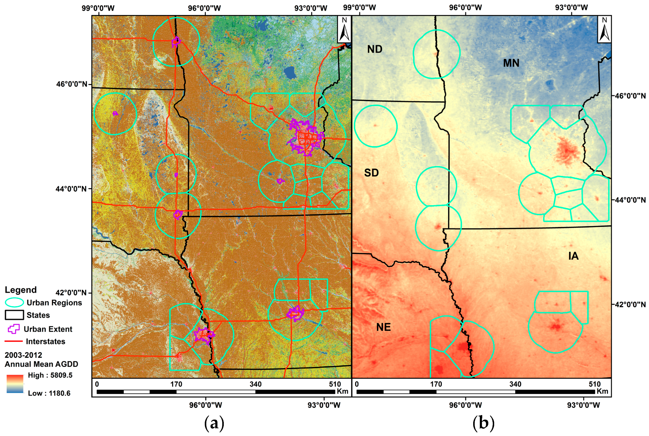
Figure 2.
(a) Example of land cover type (LCT) classification (derived from the 2011 National Land Cover Database LCT product) over Sioux Falls, SD. “Water”, “Barren”, and “Change” pixels (white) were excluded from the analyses; (b) Example of the four urban spatial subregions used in the analysis including: urban extent (UE), urban core areas (UCAs), green core areas (GCAs), and areas outside of the UE over Sioux Falls, SD.
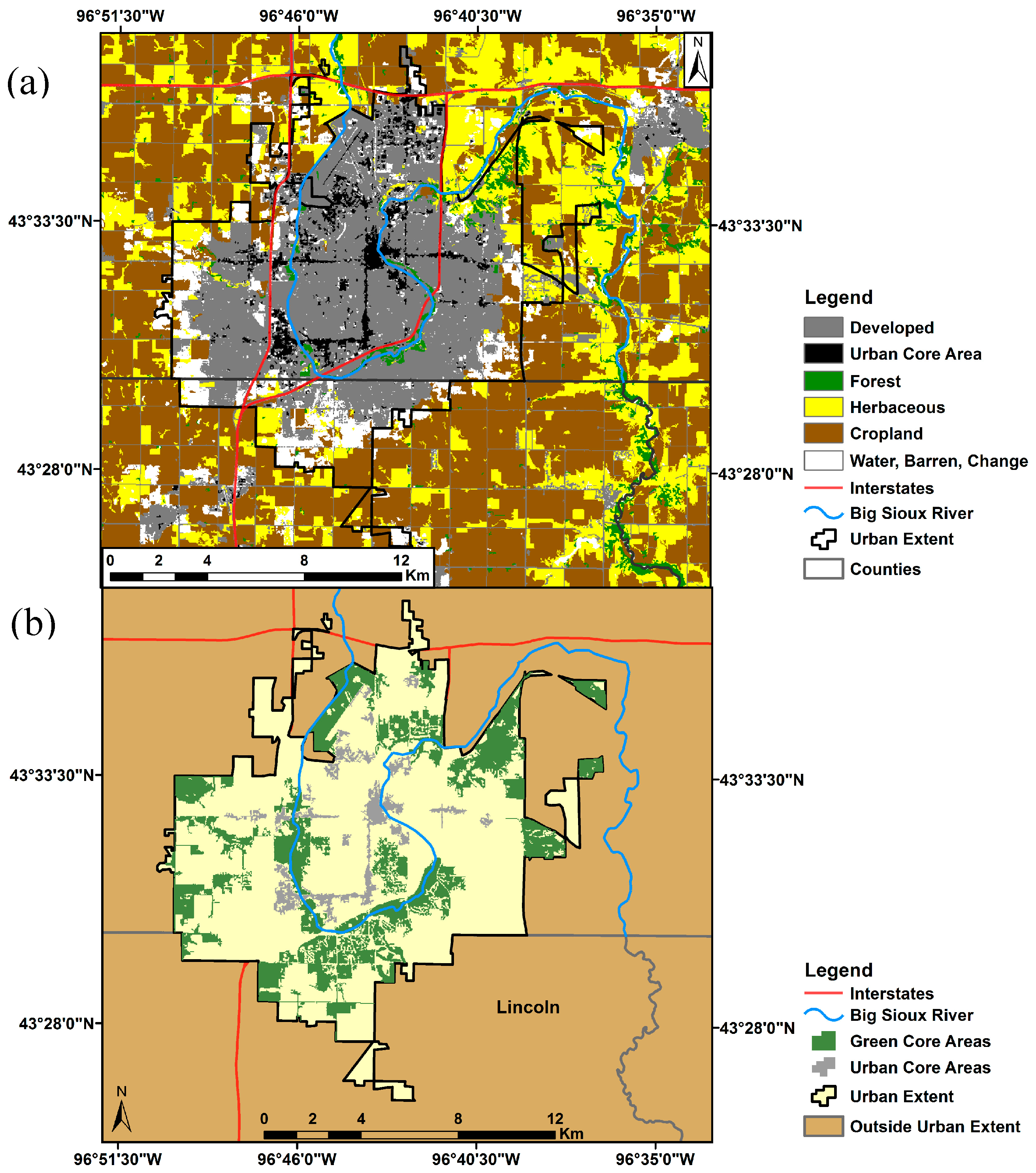
Figure 3.
Processing outline for MODIS Land Surface Temperature (LST) to accumulated growing degree-days (AGDD) algorithm that converts MODIS LST 8-day composites into annual time series of AGDD (adapted from [40]).
Figure 3.
Processing outline for MODIS Land Surface Temperature (LST) to accumulated growing degree-days (AGDD) algorithm that converts MODIS LST 8-day composites into annual time series of AGDD (adapted from [40]).

Figure 4.
Quadratic land surface phenology model fit to the 2003–2012 time series of Web-Enabled Landsat Data Normalized Difference Vegetation Index NDVI vs. MODIS Land Surface Temperature-derived accumulated growing degree-days for an example of perennial forest (green) and annual cropland (orange) pixels selected from Omaha, NE. In grey are the phenometrics derived from the model.

Figure 5.
Example of exponential trend model fit to change in duration of growing season (ΔDGSAGDD) as a function of distance from nearest urban core area for Omaha-Council Bluffs, NE-IA. The grey diamonds show where the exponential model reaches 95% of asymptotic values, used to calculate the magnitude of ΔDGSAGDD and the distance at which urban effects become insignificant. In blue is the model fit to strictly perennial vegetation land cover types and in green annual croplands are included.

Figure 6.
Results from equivalence tests between group means of duration of growing season (DGSAGDD). DGSAGDD is equivalent between green core areas (green) and urban extent (UE) areas (tan), but significantly lower in areas outside of the UE (brown) for 17 of 19 cities.
Figure 6.
Results from equivalence tests between group means of duration of growing season (DGSAGDD). DGSAGDD is equivalent between green core areas (green) and urban extent (UE) areas (tan), but significantly lower in areas outside of the UE (brown) for 17 of 19 cities.

Figure 7.
Duration of growing season (DGSAGDD) for nine study cities within the greater Minneapolis-St. Paul, MN-WI region. Water is masked (blue) and pixels with quadratic land surface phenology model fit <0.5 are in black.
Figure 7.
Duration of growing season (DGSAGDD) for nine study cities within the greater Minneapolis-St. Paul, MN-WI region. Water is masked (blue) and pixels with quadratic land surface phenology model fit <0.5 are in black.

Figure 8.
Land cover type (LCT) classification scheme for nine study cities within the greater Minneapolis-St. Paul, MN-WI region demonstrating regional differences in dominant LCT between the intensely cultivated regions in the southwest (brown) and increasingly forest/herbaceous LCTs (green/yellow) to the north and east, with the large metropolitan area of Minneapolis-St. Paul (grey) lying between the two regions.

Figure 9.
Exponential trend model fit to difference in duration of growing season (ΔDGSAGDD) as a function of distance from nearest UCA for four selected cities. Differences in ΔDGSAGDD calculated with croplands (green) and without croplands (blue) are evident, particularly in the predominantly agricultural areas surrounding Omaha-Council Bluffs, NE-IA, and Des Moines, IA, compared to rural Rochester, MN, and Minneapolis-St. Paul, MN-WI, where forests and herbaceous land covers are more widely distributed. The grey diamonds show where the exponential model reaches 95% of asymptotic values, used to calculate the magnitude of ΔDGSAGDD and the distance at which urban effects become insignificant.
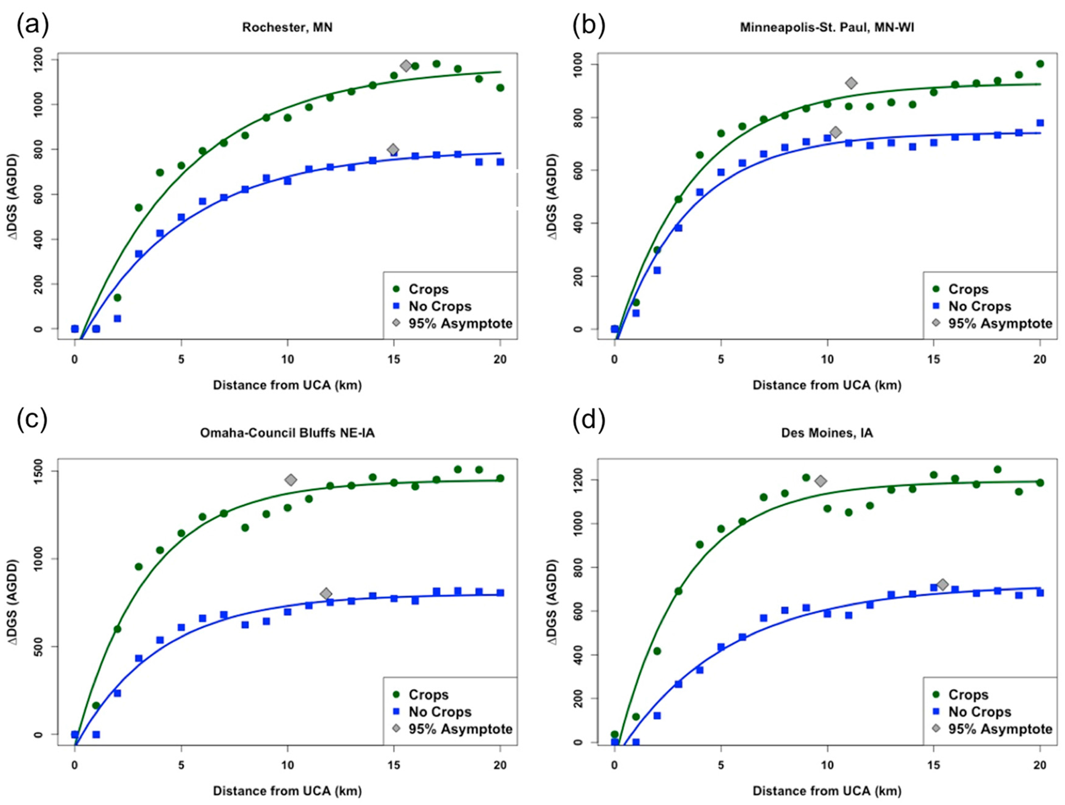
Figure 10.
Difference in duration of growing season (ΔDGSAGDD) in terms of: (a) accumulated growing degree-days (AGDD); (b) calendar days; and (c) percentage of mean DGSAGDD for results from model fit with (orange) and without (blue) croplands. Notice that ΔDGS is significantly related to latitude in terms of: total AGDD (a); but not relative (%) ΔDGS (c).

Figure 11.
Examples of linear regression model fit to PHNDVI vs. Half-TTPNDVI for four selected cities. Note the large variation in Half-TTPNDVI for croplands (yellow) and positive linear relationships seen in the three perennial vegetation land cover types.
Figure 11.
Examples of linear regression model fit to PHNDVI vs. Half-TTPNDVI for four selected cities. Note the large variation in Half-TTPNDVI for croplands (yellow) and positive linear relationships seen in the three perennial vegetation land cover types.

Table 1.
Characteristics of the 19 study cities: 2011 population [32], area of the urban extent [33], latitude, longitude, decadal mean annual accumulated growing degree-days (AGDD) calculated from the MODIS Land Surface Temperature-derived AGDD product, and percentage of pixels with land surface phenology model fit (R2) > 0.5 in each of the 19 cities.
| City | 2011 Pop. | 2010 UE (km2) | Lat | Lon | 2003–2012 AGDD | LSP Model (%) |
|---|---|---|---|---|---|---|
| MSP, MN | 3,388,716 | 2773.3 | 44.98 | −93.28 | 4318 | 66.2 |
| Omaha, NE | 876,836 | 702.4 | 41.23 | −96.03 | 5129 | 72.2 |
| Des Moines, IA | 580,779 | 519.5 | 41.62 | −93.66 | 4889 | 88.4 |
| Lincoln, NE | 306,443 | 229.1 | 40.81 | −96.68 | 5161 | 62.9 |
| Sioux Falls, SD | 232,553 | 166.2 | 43.53 | −96.74 | 4428 | 56.5 |
| Fargo, ND | 212,695 | 182.1 | 46.86 | −96.82 | 3819 | 28.6 |
| Rochester, MN | 208,446 | 131.0 | 44.02 | −92.48 | 4157 | 75.9 |
| St. Cloud, MN | 189,980 | 130.1 | 45.57 | −94.19 | 3918 | 63.8 |
| Mankato, MN | 97,280 | 68.3 | 44.17 | −93.99 | 3867 | 73.6 |
| Ames, IA | 90,834 | 59.8 | 42.03 | −93.63 | 4435 | 80.4 |
| Faribault, MN | 64,908 | 29.5 | 44.29 | −93.28 | 3996 | 82.7 |
| Marshalltown, IA | 40,967 | 29.7 | 42.04 | −92.91 | 4576 | 77.6 |
| Aberdeen, SD | 40,902 | 33.1 | 45.46 | −98.47 | 3780 | 37.8 |
| Austin, MN | 39,320 | 31.7 | 43.67 | −92.98 | 3920 | 83.2 |
| Fremont, NE | 36,943 | 28.2 | 41.44 | −96.49 | 4804 | 73.1 |
| Owatonna, MN | 36,551 | 33.0 | 44.09 | −93.22 | 4035 | 81.2 |
| Brookings, SD | 32,109 | 24.6 | 44.30 | −96.78 | 4008 | 58.3 |
| Albert Lea, MN | 31,111 | 25.5 | 43.65 | −93.37 | 3898 | 67.1 |
| Cambridge, MN | 15,155 | 25.7 | 45.54 | −93.23 | 3833 | 76.3 |
Table 2.
Summary of land cover type groupings used for classification of pixels in the study.
| National Land Cover Database Class | ID | Study Class |
|---|---|---|
| Open Water, Perennial Ice/Snow | 1 | Water |
| Developed: Open Space, Low/Medium Intensity | 2 | Developed |
| Developed: High Intensity | 3 | Urban Core Area |
| Barren Land (Rock/Sand/Clay) | 4 | Barren Land |
| Deciduous, Evergreen, Mixed Forest, Woody Wetlands | 5 | Forest |
| Shrub/Scrub, Grassland/Herbaceous, Pasture/Hay, Emergent Herbaceous Wetlands | 6 | Herbaceous |
| Cultivated Crops | 7 | Cropland |
| Change in Impervious Surface Area: 2001–2006 | 8 | 2001–2006 Change |
| Change in Impervious Surface Area: 2006–2011 | 9 | 2006–2011 Change |
Table 3.
Scaling parameters of exponential trend model for difference in duration of growing season (ΔDGSAGDD) fit with croplands included (“C”) and with croplands excluded (“NC”) as well as the magnitude of ΔDGSAGDD (“a”, in accumulated growing degree-days) and distance where urban influence on the surrounding environment becomes insignificant, measured from nearest urban core area.
| City | NC b | C b | C u | NC u | C R2 | NC R2 | NC a | C a | ∆a | NC Dist (km) | C Dist (km) |
|---|---|---|---|---|---|---|---|---|---|---|---|
| Aberdeen, SD | 0.233 | 0.204 | 0.887 | 0.848 | 0.904 | 0.857 | 528 | 836 | 309 | 12.9 | 14.7 |
| Albert Lea, MN | 0.243 | 0.251 | 1.151 | 1.174 | 0.934 | 0.879 | 652 | 1135 | 482 | 12.3 | 12.0 |
| Ames, IA | 0.217 | 0.264 | 1.097 | 1.154 | 0.963 | 0.899 | 662 | 1400 | 738 | 13.8 | 11.4 |
| Austin, MN | 0.258 | 0.374 | 0.974 | 0.991 | 0.953 | 0.878 | 689 | 1203 | 514 | 11.6 | 8.0 |
| Brookings, SD | 0.399 | 0.369 | 1.069 | 1.050 | 0.952 | 0.964 | 605 | 1084 | 480 | 7.5 | 8.1 |
| Cambridge, MN | 0.275 | 0.396 | 1.003 | 0.984 | 0.910 | 0.951 | 422 | 482 | 60 | 10.9 | 7.6 |
| Des Moines, IA | 0.195 | 0.310 | 1.065 | 1.109 | 0.961 | 0.975 | 721 | 1195 | 474 | 15.4 | 9.7 |
| Faribault, MN | 0.388 | 0.419 | 1.004 | 1.145 | 0.966 | 0.920 | 545 | 970 | 426 | 7.7 | 7.2 |
| Fremont, NE | 0.253 | 0.373 | 0.777 | 0.970 | 0.970 | 0.933 | 735 | 1467 | 732 | 11.8 | 8.0 |
| Lincoln, NE | 0.276 | 0.317 | 0.792 | 0.900 | 0.944 | 0.968 | 855 | 1303 | 448 | 10.9 | 9.5 |
| Mankato, MN | 0.238 | 0.312 | 1.032 | 1.068 | 0.946 | 0.963 | 393 | 931 | 538 | 12.6 | 9.6 |
| Marshalltown, IA | 0.221 | 0.178 | 0.896 | 1.007 | 0.987 | 0.970 | 804 | 1428 | 623 | 13.6 | 16.8 |
| MSP, MN | 0.289 | 0.270 | 1.058 | 1.094 | 0.975 | 0.975 | 743 | 929 | 186 | 10.4 | 11.1 |
| Omaha, NE | 0.254 | 0.296 | 1.042 | 1.089 | 0.972 | 0.963 | 800 | 1449 | 649 | 11.8 | 10.2 |
| Owatonna, MN | 0.357 | 0.451 | 1.101 | 1.089 | 0.937 | 0.937 | 754 | 1276 | 522 | 8.4 | 6.6 |
| Rochester, MN | 0.201 | 0.193 | 1.090 | 1.124 | 0.966 | 0.966 | 799 | 1172 | 374 | 15.0 | 15.6 |
| Sioux Falls, SD | 0.238 | 0.340 | 1.097 | 1.109 | 0.960 | 0.956 | 832 | 1375 | 543 | 12.6 | 8.8 |
| St. Cloud, MN | 0.532 | 0.527 | 1.065 | 1.085 | 0.924 | 0.940 | 497 | 611 | 115 | 5.6 | 5.7 |
| Minimum | 0.195 | 0.178 | 0.777 | 0.848 | 0.904 | 0.857 | 393 | 482 | 60 | 5.6 | 5.7 |
| Maximum | 0.532 | 0.527 | 1.151 | 1.174 | 0.987 | 0.975 | 855 | 1467 | 738 | 15.4 | 16.8 |
| Mean | 0.281 | 0.325 | 1.011 | 1.055 | 0.951 | 0.939 | 669 | 1125 | 456 | 11.4 | 10.0 |
© 2017 by the authors. Licensee MDPI, Basel, Switzerland. This article is an open access article distributed under the terms and conditions of the Creative Commons Attribution (CC BY) license (http://creativecommons.org/licenses/by/4.0/).
Share and Cite
MDPI and ACS Style
Krehbiel, C.; Zhang, X.; Henebry, G.M. Impacts of Thermal Time on Land Surface Phenology in Urban Areas. Remote Sens. 2017, 9, 499. https://doi.org/10.3390/rs9050499
AMA Style
Krehbiel C, Zhang X, Henebry GM. Impacts of Thermal Time on Land Surface Phenology in Urban Areas. Remote Sensing. 2017; 9(5):499. https://doi.org/10.3390/rs9050499
Chicago/Turabian StyleKrehbiel, Cole, Xiaoyang Zhang, and Geoffrey M. Henebry. 2017. "Impacts of Thermal Time on Land Surface Phenology in Urban Areas" Remote Sensing 9, no. 5: 499. https://doi.org/10.3390/rs9050499
Note that from the first issue of 2016, this journal uses article numbers instead of page numbers. See further details here.