
Examining Forest Disturbance and Recovery in the Subtropical Forest Region of Zhejiang Province Using Landsat Time-Series Data

1
The Nurturing Station for the State Key Laboratory of Subtropical Silviculture, Key Laboratory of Carbon Cycling in Forest Ecosystems and Carbon Sequestration of Zhejiang Province, School of Environmental & Resource Sciences, Zhejiang Agriculture and Forestry University, Lin An 311300, China
2
Center for Global Change and Earth Observations, Michigan State University, East Lansing, MI 48823, USA
*
Author to whom correspondence should be addressed.
Remote Sens. 2017, 9(5), 479; https://doi.org/10.3390/rs9050479
Submission received: 14 March 2017
/
Revised: 3 May 2017
/
Accepted: 10 May 2017
/
Published: 14 May 2017
Abstract
:Detection of forest disturbance and recovery has received much attention during the last two decades due to its important influence on forest carbon budget estimation. This research used Landsat time-series data from 1984 to 2015 to examine forest disturbance and recovery in a subtropical region of eastern Zhejiang Province, China, through the LandTrendr algorithm. Field inventory data and high spatial resolution images were used to evaluate the disturbance and recovery results. This research indicates that high producer and user accuracies for both disturbance and recovery classes were obtained and three levels of disturbance and recovery each can be detected. Through incorporation of climate data and disturbance results, drought events also can be successfully detected. More research is needed to incorporate multisource data for detection of forest disturbance types in subtropical regions.
1. Introduction
Forest ecosystems are often disturbed by physically induced (e.g., drought, fire) and human-induced (e.g., selective logging, clear-cutting) factors, resulting in high uncertainty in forest carbon budget estimation [1,2,3,4]. Due to high forest coverage and relatively young forest ages, the subtropical region of China has become an important carbon sink [5] and has played an important role in the global carbon budget [6]. However, high population density, economic conditions, and frequent natural disasters (e.g., drought, flooding) in this region generate frequent disturbances, which can result in uncertain carbon estimation if the disturbances are not taken into account. Timely and accurate detection of forest dynamic change [6,7] is required to better understand its contribution to reducing the uncertainty of carbon budget estimation.
Forest disturbance is a discrete event caused by a significant change in the physical environment in a forest ecosystem, a community, or a species structure [8]. The disturbance can originate from natural events such as forest fire, drought, flooding, insect pests, and freezing, or human-induced factors such as deforestation, selective logging, and mining. Forest disturbance can be destructive, resulting in significant damage to the forest structures and degradation of ecological functions [9]. Conversely, forest recovery can be natural, a process of natural vegetation succession, or artificial, gradual recovery through forest management such as the alteration of inefficient forests [2].
In general, forest disturbance and recovery information can be obtained through field inventory or remote sensing technologies. Field surveys are the most accurate approach to examine forest disturbance or recovery, but the time-consuming and labor-intensive work and difficulty in accessing some sites in mountainous regions make it only feasible for accessible sites with small areas. On the other hand, remote sensing, especially optical sensor data, due to its long-term data availability and repeated acquisition capability at the same location, has become one of the most important data sources for detecting forest disturbance in a large area [10,11]. Many studies have been conducted for forest disturbance assessment at the global scale using coarse spatial resolution images (e.g., Advanced Very High Resolution Radiometer (AVHRR) and Moderate Resolution Imaging Spectroradiometer (MODIS)) [12,13,14,15] and at the regional scale using medium spatial resolution data (e.g., Landsat) [9,16,17,18,19,20]. Detection of forest disturbance can be based on a comparison between two or more dates of remote sensing images and many change detection approaches can be used for this purpose, as summarized in previous literature review publications (e.g., [21,22]). Banskota et al. [11] provided an overview of forest monitoring approaches using Landsat time-series data, including the description of image preprocessing, selection of remote sensing variables, and related algorithms. The critical steps are to identify suitable variables and a relevant algorithm for conducting the change detection [10].
In theory, forest disturbance and recovery can cause differences in canopy structures; thus, optical sensor data may have different surface reflectances or radar data may have different backscatter coefficients for the sites with disturbance or recovery. Therefore, remote sensing technologies can be used to detect forest disturbance and recovery if proper approaches are used, including suitable variables and corresponding algorithms. Different variables, such as spectral bands, vegetation indices, image transform, and subpixel features may be used [10,11]. For example, the Landsat shortwave infrared (SWIR) image is sensitive to moist condition, and it has been used for detecting forest disturbance [19] because the change of forest structures due to disturbance can result in the change in moist structures (e.g., moisture, canopy-cast shadows). However, individual spectral bands are often influenced by external factors such as topographic factors and atmospheric conditions; vegetation indices can reduce these impacts [10]. Therefore, a vegetation index such as normalized difference vegetation index (NDVI), normalized difference water index (NDWI), or normalized burned ratio (NBR) and Tasselled cap wetness are often used for forest disturbance detection [23,24,25,26]. In addition to the pixel-based variables, spatial-based features such as textures and segmentation have been used for land-cover change detection [21,27,28,29] but have not been extensively used for forest disturbance detection. The major reason may be that the spatial features reduced the small differences caused by forest disturbance or recovery, and the patch sizes and complexity of tree species affect the selection of suitable spatial features [30]. Other potential variables are the subpixel features that are decomposed from multispectral bands using spectral mixture analysis [31]. A new index based on the unmixed subpixel features (e.g., green vegetation, shade, and non-photosynthetic vegetation) can further improve the detection of forest disturbance, like the hickory forest disturbance caused by extreme drought events in Zhejiang Province in 2013 [31].
Another critical step in forest disturbance analysis is to select a suitable algorithm. Previous publications e.g., [10,21,22,32] summarized many detection techniques for land-cover change, and these techniques can also be used for forest disturbance detection. In recent years, new approaches such as Vegetation Change Tracker (VCT), Landsat-based Detection of Trends in Disturbance and Recovery (LandTrendr), and Breaks For Additive Season and Trend Monitor (BFAST) were developed for forest disturbance detection based on Landsat time-series data [11,23,24,25,26,32,33]. For example, curve fitting was used to detect forest disturbance and recovery in western Oregon, USA, with Landsat Thematic Mapper/Enhanced Thematic Mapper Plus (TM/ETM+) time-series images [34,35,36]. Thresholding-based approaches with the Tasselled cap–derived disturbance index or subpixel variables also have been used to detect forest disturbance [1,31,37,38]. VCT [17,18,39,40] is also a threshold-based approach for detection of forest disturbance using the integrated forest Z-score index (IFZ) from Landsat time-series data. Selection of proper thresholds is critical for successfully detecting forest disturbance and recovery; thus, it often depends on ground-truth data and the skills of the analyst. In recent years, the two algorithms LandTrendr [24,41,42,43,44,45] and BFAST [16,33,46,47] often have been used to detect forest disturbance and recovery in North America. There are also other algorithms such as Continuous Change Detection and Classification (CCDC) [48] and Continuous Monitoring of Forest Disturbance Algorithm (CMFDA) [9]. Different algorithms have their own merits and shortcomings in forest disturbance detection, but it is unclear which one has the best performance for a specific study area. It also is a challenge to validate forest disturbance assessments due to difficulty in collecting ground-truth data. High spatial resolution images such as QuickBird with a multitemporal scale were often used for this validation, presenting an overall accuracy of 60%–80% [17,18,19,41].
Forest change can be grouped into three broad categories: abrupt, moderate, and slight. Abrupt change is similar to land-cover conversion, the complete change from one land cover to another; for example, from forest to cropland or pasture or buildings, from bare soils to plantations. The detection of deforestation and afforestation using remote sensing techniques is relatively easy because of the significant difference in spectral signatures in optical sensor data. The challenge is to detect the moderate and slight changes (or modifications)—changes in quantitative values without change in types—for example, the forest change due to selective logging, insect disease, and drought. Moderate change shows an obvious difference in forest canopy structures caused by external factors (e.g., extreme weather, human activities), resulting in obvious change from before to after the event. Remote sensing technologies can detect moderate change; for example, Meddens et al. [49] detected bark beetle–caused tree mortality using single-date and multidate Landsat imagery in north-central Colorado and southern Wyoming, Schwantes et al. [50] quantified drought-induced tree mortality in the open canopy woodlands of central Texas using a Landsat time series; Jarron et al. [25] differentiated different levels of harvesting practices using annual Landsat time-series data in central British Columbia, Canada. The biggest challenge in using remote sensing technology is to detect the slight forest change, which may be caused by such factors as selective logging or a drought event, resulting in gradual degradation or recovery in a relatively short time. This kind of detection requires careful selection of remote sensing time-series data, suitable variables, and algorithms. For example, Meigs et al. [23] examined the detection of four subtle change types: short-duration decline then recovery; short- then long-duration decline; long-duration decline; and long-duration decline then recovery using the LandTrendr algorithm in Oregon, USA. Lambert et al. [51] monitored forest decline through remote sensing time-series analysis in southwestern Massif Central Mountains, France. Chen et al. [52] detected the gradual tree line movement in Tianshan Mountain, China, using spectral mixture analysis based on multitemporal Landsat multispectral images.
Many previous studies on forest disturbance assessments have focused on coniferous forests and mixed evergreen and deciduous forests in North America [9,17,18,19,24,48,53,54]. In the subtropical forest regions of China, detection of forest disturbance and recovery has not received much attention. The major reasons may be (1) the complex landscape and species composition; (2) complex impacts of different physically and human-induced factors such as selective logging, extreme weather, and insect disease on forest disturbance, resulting in difficulty in detecting forest disturbance in this region. Therefore, the objective of this research is to explore the detection of forest disturbance and recovery levels in the subtropical region in Zhejiang Province using the LandTrendr algorithm based on Landsat time-series data.
2. Materials and Methods
2.1. Study Area
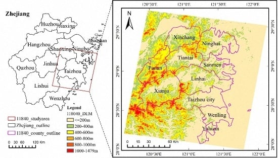
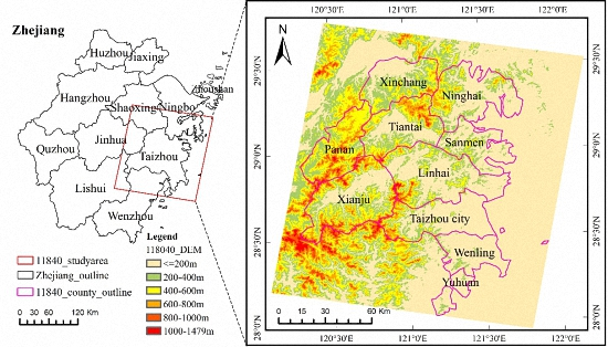
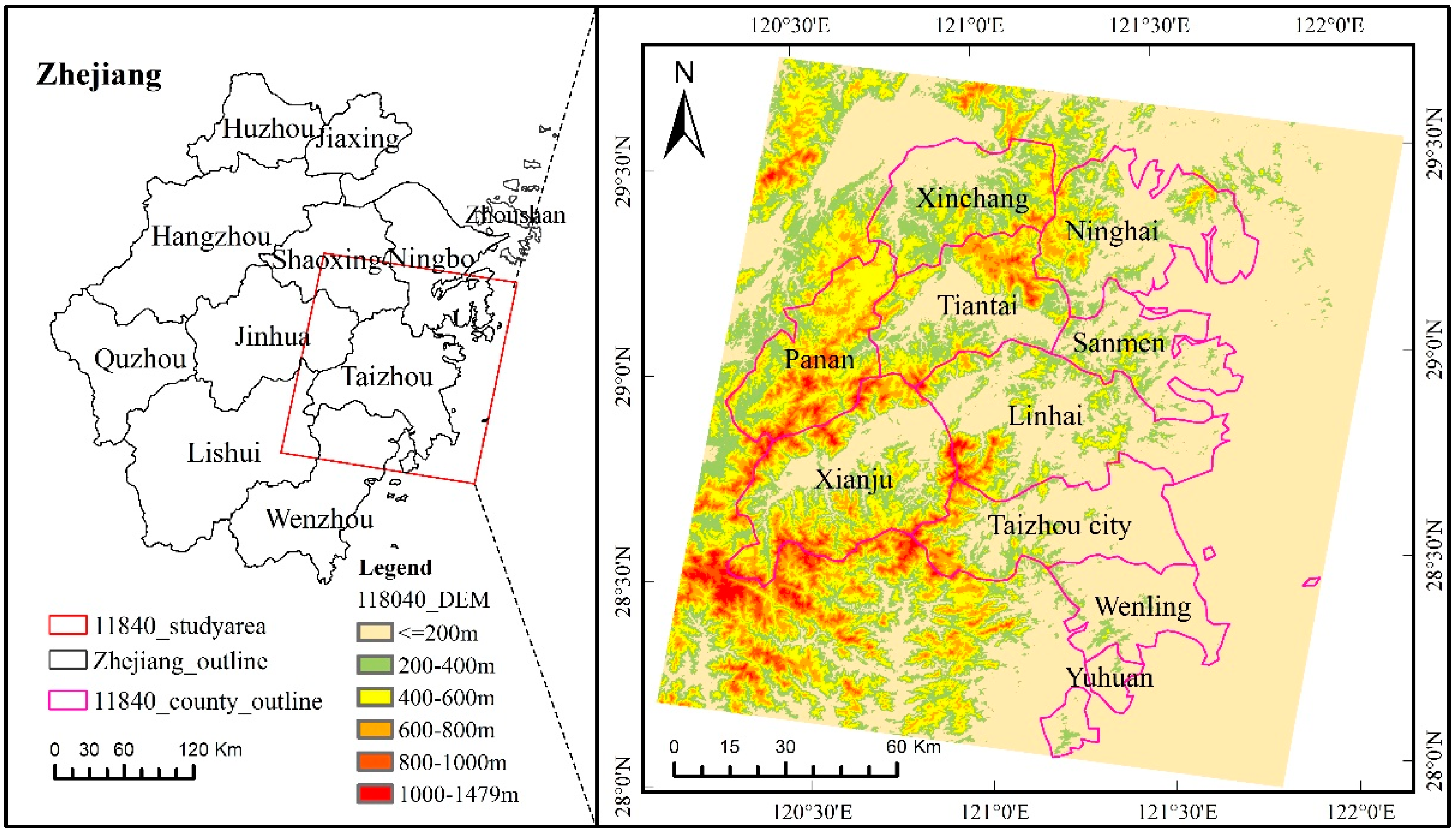
The study area is located in the eastern coastal area of Zhejiang province, China (Figure 1). This region belongs to the subtropical monsoon climate zone presenting four distinct seasons. The Terrain is undulating, flat, and low elevation areas in the coastal region in the east and mountains with elevations as high as 1470 m in the southwest region. This study area had high forest coverage of 62.2% in 2000 and included broadleaf, coniferous, and mixed forests, as well as bamboo. Major afforestation began in the late 1970s and continued until the late 1990s in the mountainous regions.
The population density and economic conditions decline from the coastal region to the mountainous regions. In the past three decades, rapid urbanization, especially in coastal regions, has resulted in a large conversion from agriculture land to impervious surfaces [55]. The rapid population migrations from rural to urban and relevant urban expansion have accelerated the conflict between land needs for urban construction and farmlands for food production. In order to keep the agricultural area stable for food production, the government issued policies stating that loss of agriculture areas in one place had to be complemented from other places, resulting in deforestation in mountainous regions [56]. Therefore, the rapid urbanization in coastal regions has resulted in high conversion of forest land to agricultural land in mountainous regions, but the land quality for agriculture is often poor.
This study area is vulnerable to natural disasters. The main weather disasters are intense rain and low temperatures in the spring season, typhoon, hail, and high temperatures in summer, droughts in fall, and flooding in the rainy season. According to the Taizhou Statistical Yearbook records, high temperatures and droughts in summer is an important factor resulting in forest disturbance; other natural disasters such as typhoons, flooding, and hail have limited effects on forest disturbance. In contrast, human-induced factors such as deforestation and selective logging seriously affect forest disturbance, while afforestation and forest management promote forest recovery.
2.2. Data Preparation
Different datasets were collected and used in this research (Table 1). Landsat TM/ETM+/Operational Land Imager (OLI) imagery from 1984 to 2015 was selected based on the consideration of data availability, quality, and similar vegetation phenology. In this subtropical region, frequent cloud cover is a major problem restricting image collection. For example, no images were available between 1993 and 1998 in this study area. This problem affects the effective detection of forest disturbance because forests can be quickly restored if growth conditions such as temperature and moisture are suitable. After all Landsat images were collected, one important step was to convert the digital number to surface reflectance. The Landsat Ecosystem Disturbance Adaptive Processing System (LEDAPS) algorithm provided the approach to conduct the radiometric and atmospheric calibrations for all Landsat TM and ETM+ images [57]. Because LEDAPS did not provide the atmospheric calibration algorithm for Landsat 8 OLI data, a similar approach was used for that data [20]; that is, the radiometric calibration was conducted using ENVI 5.1 software (Research Systems Inc., Boulder, CO, USA). Then, a second simulation of the satellite signal in the solar spectrum (6S) model was used to conduct atmospheric calibration for which the relevant parameters were from the Landsat ETM+ data [58]. The calibrated results between OLI and ETM+ were compared to make sure the unchanged forest sites at the same locations had similar surface reflectance values.
The Tasselled cap transformation algorithm [59,60] was used to transform Landsat multispectral bands into three components: brightness, greenness, and wetness. The Fmask algorithm was used to mask cloud and shadow of time-series images to eliminate their influence on the LandTrendr temporal segmentation algorithm [61,62]. NDVI was used to distinguish impervious surfaces, bare soils, and water bodies from vegetation (forest and non-forest vegetation such as croplands). Phenology information of croplands based on different seasons of Landsat images was used to further separate croplands and forests. Direct separation of croplands and forests based on spectral signatures of a single-season Landsat image is often difficult. In this study area, croplands have three types: (1) planting in spring and harvesting in fall; (2) planting in winter and harvesting in summer; and (3) greenness in both spring and fall seasons. Based on Landsat OLI images in winter 2014 and summer 2015, sample plots for the three cropland types were selected, and the matched filtering approach [63] was used to extract the croplands. Meanwhile, elevation and slope from digital elevation model (DEM) data was further used to modify the results because cropland is usually distributed in the regions with slopes of less than 10° and elevation of less than 600 m. Climate and forest inventory data were used to examine forest disturbance by combining the LandTrendr-detected disturbance results.
2.3.Detection of Forest Disturbance and Recovery
The LandTrendr time segmentation algorithm has been regarded as a good approach to effectively detect forest disturbance and recovery [41,64]; thus, it was used in this study. Through the extraction of the surface reflectance change trend from the time-series data, the LandTrendr algorithm can capture short-term disturbance and long-term recovery trend. A detailed description of this algorithm can be found in previous publications (e.g., [41]). Previous research also indicated that the NBR is more sensitive to disturbance events than the NDVI and TCW (wetness component of the Tasselled cap transformation). Therefore, this research selected NBR to detect forest disturbance and recovery. The NBR is calculated as
where NIR and SWIR are near infrared (850–880 nm) and shortwave infrared (1570–1650 nm) reflectance. The normalized reflectance time-series images, the Tasselled cap transformed components, and the cloud and shadow mask images were used as input to the LandTrendr model. The model control parameters were obtained using the approach described in [41]. The major output includes the NBR value, years of change vertices, the duration and the change amount of every segment. Based on the LandTrendr results, three classes—disturbance, recovery, and stable (no-change)—were classified [41].
NBR = (NIR − SWIR)/(NIR + SWIR)
Two approaches—forest inventory data and visual interpretation—were then used to evaluate the LandTrendr results. A total of 261 permanent plots with plot size of 800 m2 were measured in 1994, 1999 and 2004, and were used as reference data for accuracy assessment. Based on surveyed items such as forest type, dominant tree species, forest ages, average canopy height, and average diameter at breast height (DBH), we evaluated each plot between two inventory dates to decide whether the plot was in one of the three classes: disturbance, recovery, or stable. The surveyed sample plots were linked to the corresponding locations from the LandTrendr results to produce an error matrix. An alternative is to use the Timesync visual interpretation method [42]. Samples were randomly selected and allocated on the LandTrendr results, and each plot was visually examined to determine the disturbance year and level (disturbance, recovery, or stable) using time-series analysis with high spatial resolution images between 2004 and 2015 from Google Earth. Because some points cannot be determined due to different factors such as clouds and image quality, these points were removed; thus, 306 samples were finally selected for validation.
2.4. Determination of Disturbance and Recovery Levels
In order to further examine forest disturbance severity, three disturbance levels of serious, moderate, and light were classified. In this research, 32 sample plots were used to determine the thresholds through the analysis of mean and standard deviation of the dNBR (mean− 2*std, mean+ 2*std); here, dNBR represents the NBR difference of two images between neighboring dates and std represents standard deviation. The thresholds for recovery levels are the opposite of disturbance levels. Table 2 summarizes three disturbance and recovery categories, each based on these thresholds.
As Table 1 indicated, not every year has Landsat images due to the cloud-cover problem in this study area. Based on the Landsat data availability, this study was first analyzed in five time periods: 1987–1993, 1993–1998, 1998–2004, 2004–2010 and 2010–2015, for the sake of result presentation in temporal distribution. The statistical analysis of disturbance and recovery areas was then analyzed at the real-time periods of one, two, three or five years, depending on the data availability. For comparison of the changed areas of disturbance and recovery levels, annual change areas were calculated. Meanwhile, the climate data (e.g., temperature and precipitation in July) were linked to the disturbance and recovery results for exploring the drought-induced forest disturbances.
3. Results
3.1. Analysis of LandTrendr Results
The accuracy assessment results based on forest inventory samples and visual interpretation separately (Table 3) indicated that the LandTrendr approach can effectively detect forest disturbance and recovery classes. Both accuracy assessment results show high producer and user accuracies for disturbance and recovery classes but have very low user accuracy for the stable class. There is a high amount of confusion between the stable and recovery classes; that is, many samples of recovery class were misclassified to stable class. For some forest inventory samples, we assume that the forest is in recovery state due to natural growth, but Landsat cannot effectively detect its change in spectral signatures due to the data saturation problem caused by remote sensing data limitation. In contrast, for some forest samples, we cannot clearly decide if it is in recovery state or stable state through visual interpretation because of their similar color and spatial structure. However, the high producer and user accuracies for both disturbance and recovery categories imply that the approach used in this research is robust.
3.2. Spatial and Temporal Patterns of Forest Disturbance and Recovery
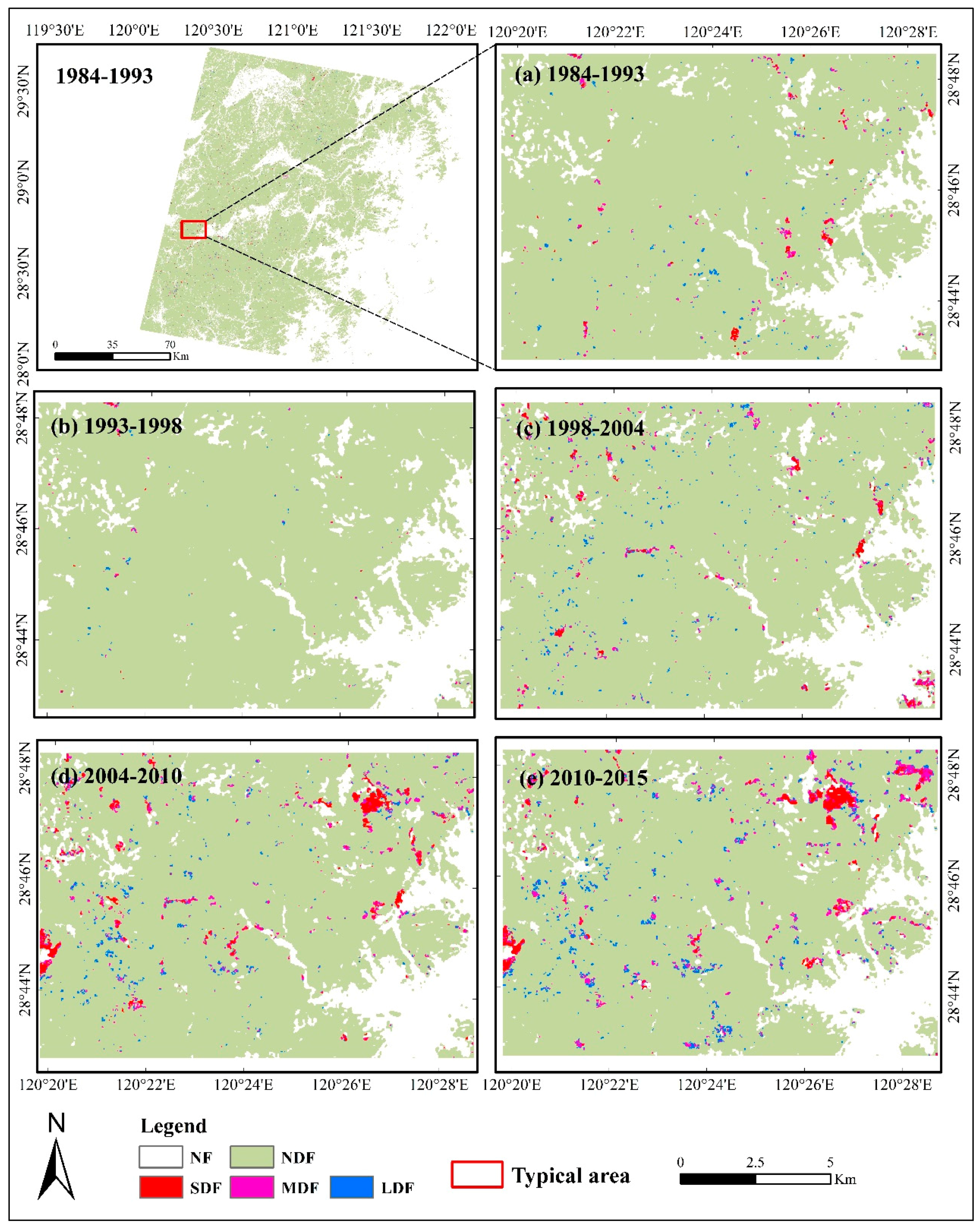
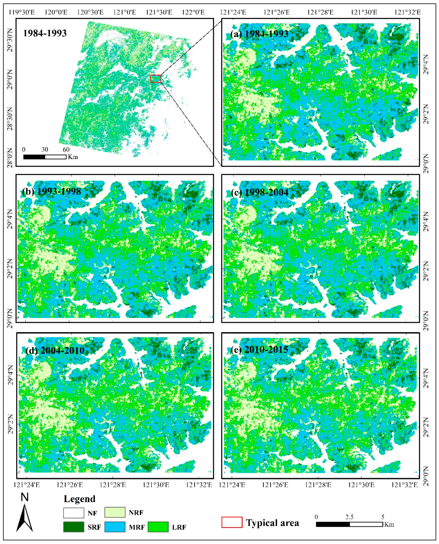
The spatial distribution of forest disturbance in Figure 2 indicates that forest disturbance occurred dispersedly. The forests closer to the urban regions or roads resulted in higher frequency of disturbance. Overall, light disturbance is widely distributed with small patch sizes; serious and moderate disturbances show large patches. In contrast, the study area is occupied by the recovery classes, especially the light- and medium-recovery classes (see Figure 3), implying that forests in this study area were expanded or in continuous growth during the change detection periods. The statistical results for different levels of disturbance and recovery during various detection periods (Table 4) indicate that the disturbance area is much smaller than recovery area, the areas of different disturbance levels are slightly increased overall, but the areas of recover levels remained relatively stable. The annual disturbance rate during 2010–2015 was especially higher than in any other period. One interesting thing is that the disturbance areas in 1993–1998 were much smaller than in any other period, but the recovery areas were larger. This is caused by the data problem that longer intervals between Landsat images (see Table 1 about the image acquisition dates) result in an inability to detect disturbance but an ease with detecting recovery class, implying the requirement of dense images for detection of disturbance.
3.3. Analysis of Statistical Data of Forest Disturbance and Recovery
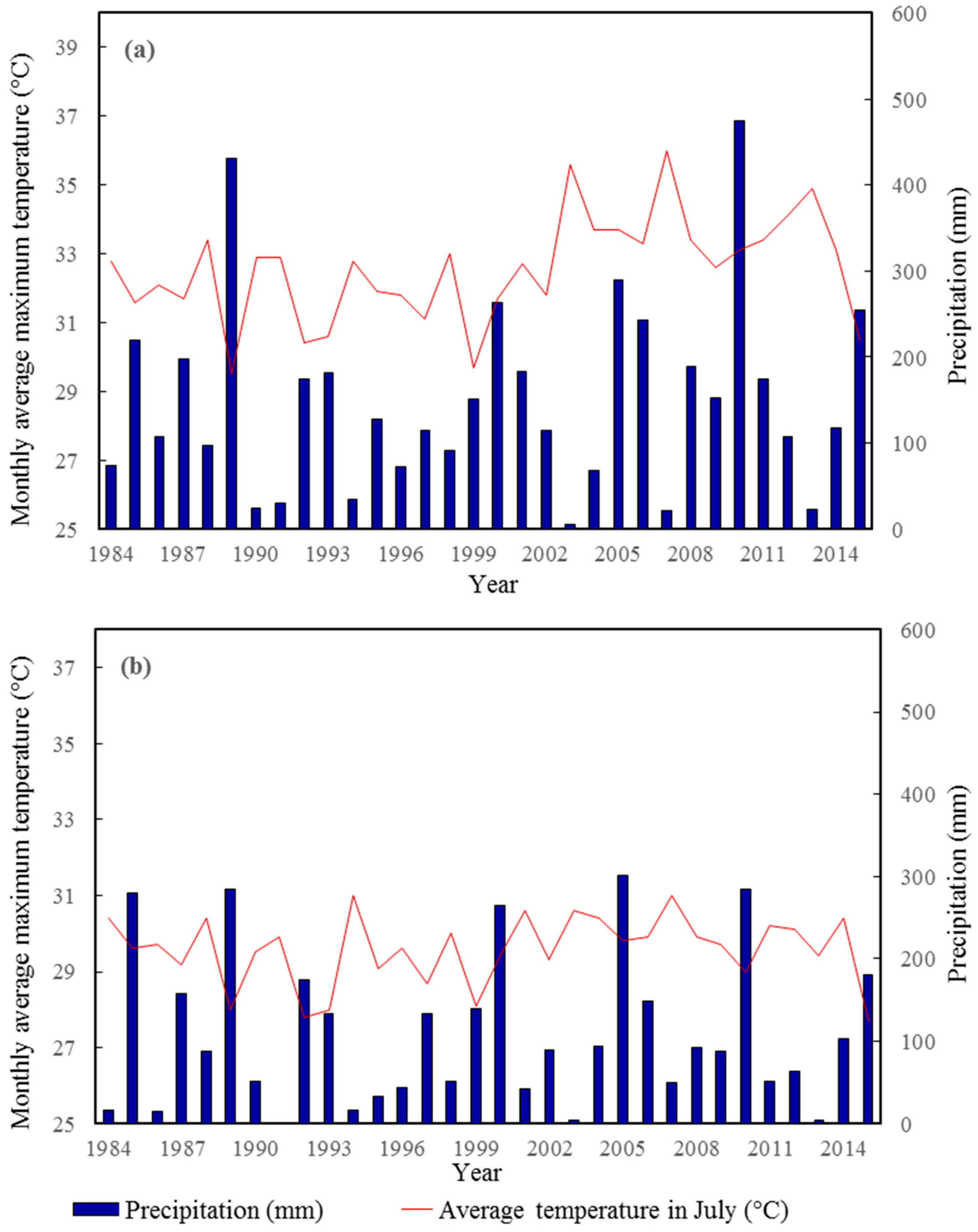
The statistical results of the disturbance and recovery areas (Table 5) indicate that the disturbance areas for certain years have much higher values than in other years; for example, the periods of 2002–2003 and 2003–2004, 2010–2013 and 2013–2015 have much higher disturbance areas than other periods. Recovery areas have a similar situation. If the disturbance and recovery areas in Table 5 are linked to drought events (high temperature and low precipitation in Figure 4), the years of high disturbance areas coincide with the years of drought, implying that drought events can be successfully detected using the LandTrendr approach. In addition, this implies that drought events are an important factor resulting in forest disturbance in this region. For example, Figure 4 indicates that 1991, 2003 and 2013 had the most drought; thus, the areas with the highest disturbance for these years and following years were detected, with forest recovery areas often appearing one year later. Table 5 also indicates that the optimal detection period is one or two years. The five-year period is too long to effectively detect disturbance and recovery. As shown in Table 5, the annual change area due to disturbance and recovery in 1993–1998 is much smaller than in other neighboring years. This is reasonable in that forest growth is dynamic; thus, forest disturbance due to selective logging or drought can be restored in months or years.
4. Discussion
This research shows that LandTrendr can effectively detect disturbance and recovery categories with high producer and user accuracies based on Landsat time-series data in a subtropical region. This research also indicates that the detection of forest disturbance and recovery is a comprehensive procedure that requires consideration of different factors such as collection of ground-truth data, definitions of disturbance and recovery classes, selection of suitable remote sensing variables and optimization of parameters used in the algorithm, and evaluation of detected disturbance and recovery results. In particular, selection of suitable variables and corresponding algorithm is critical for successful detection of forest disturbance and recovery classes.
Different remote sensing variables, such as Landsat SWIR [19], NBR [23,24], Wetness from Tasselled cap transform [24,25], and subpixel features [31] have been used for detection of forest disturbance. In particular, vegetation indices have been regarded as a better variable than individual spectral bands because they can reduce the impacts of external factors such as topography and atmosphere on the surface reflectance and can enhance some specific features such as forest structure characteristics [10,65]. For example, previous research on forest disturbance studies in North America has proven that NBR is more sensitive than traditional indices such as NDVI [23,24]. However, vegetation indices have a data saturation problem; that is, when forest canopy density reaches a certain value, NDVI values become the same even if forest biomass continued to increase [66]. The fraction image from the decomposing multispectral imagery can improve the performance for forest disturbance, as shown in a detection of drought-induced disturbance of hickory plantations [31]. In reality, the disturbance caused by different factors such as selective logging and insect disease have different influences on the forest canopy features; thus, it may require identifying a specific vegetation index for the forest disturbance detection. It is unclear that NBR is the best for subtropical regions because of the different compositions of tree species and different disturbance factors in a large area. More research is needed to identify an optimal vegetation index suitable for subtropical regions.
The quality of remote sensing data is an important factor influencing forest disturbance. In subtropical regions, the frequent cloud cover is a big problem resulting in a lack of Landsat images due to its relatively infrequent revisit dates. For example, there are no Landsat images for the years between 1993 and 1998. Most of the disturbances caused by such factors as drought and selective logging can be restored within one or two years; thus, such a disturbance cannot be detected if the detection period is more than two years because vegetation is growing and restoring. This situation is shown in Table 5: the detected disturbance and recovery areas are much smaller in 1993–1998 than in any other period in this study. For certain years of images, we could not find cloud-free images; thus, we had to combine several images to produce a new image, which influenced the surface reflectance. In the future, more research should be done to develop an algorithm that can effectively integrate the use of different optical sensor data such as CBERS, ASTER, or SPOT if the same sensor data without clouds are not available.
In addition to selection of suitable variables with dense dates, different algorithms such as VCT, LandTrendt, and BFAST have been developed for detection of forest disturbance and recovery [11,23,24,25,26,32,33], but their performances vary, depending on many factors such as the composition of forest species and complexity of the landscape under investigation, the variables used, and parameters in the algorithm. For example, several control parameters are used in the LandTrendr algorithm and they need to be optimized. It is critical to identify optimal parameters for producing the best detection results. Thus, ground-truth data are very important, but they are often difficult to collect in the field. In the past decade, high spatial resolution images such as QuickBird, Pleiades, and Worldview have been available to partially replace ground-truth data.
Validation of the disturbance results is often a challenge, especially for historical data. In this research, we collected sample plots that had been measured in 1994, 1999 and 2004. We were able to determine whether the plot was disturbed or restored based on the calculation of volume or biomass to see whether the amount increased or decreased, but the change may be small due to some disturbance such as drought. For example, Figure 4 indicates that there was a drought event in 1994, but we do not have Landsat images for 1994–1997; thus, much disturbance that occurred after 1993 and before 1998 cannot be detected. Even if we can use high spatial resolution images for the latest decade, it is still difficult to visually interpret the places where small disturbances or growth occurred, and this is one reason why the stable and recover classes can be confused. That is, many samples with recovery were wrongly interpreted as stable.
5. Conclusions
The subtropical forest region in China is an important part in influencing the global carbon budget. The high population density and intense physically induced and human-induced factors lead to high forest disturbance, requiring detection of forest disturbance and recovery at long temporal scales. This research used the LandTrendr algorithm to examine forest disturbance and recovery distribution with high accuracy. The major conclusions can be summarized as follows:
- (1)
- LandTrendr algorithm can effectively detect forest disturbance and recovery classes, but dense Landsat time-series data are required for accurately extracting the disturbance and recovery features;
- (2)
- ground-truth data are critical to determine disturbance and recovery levels through identification of suitable thresholds, but are often unavailable; thus, high spatial resolution images with multiple temporal scales are very helpful;
- (3)
- forest disturbance and recovery detection is a comprehensive procedure that requires good design of different steps: collection of ground-truth data, selection of time-series remote sensing variables, algorithm, and evaluation of the results;
- (4)
- more research is needed to integrate multisource data for forest disturbance and recovery detection, especially in subtropical and tropical regions due to the frequent cloud-cover problem.
Acknowledgments
This study was financially supported by the National Natural Science Foundation of China (Grant No. 41571411) and the Zhejiang Agriculture and Forestry University’s Research and Development Fund (Grant No. 2013FR052).
Author Contributions
Dengsheng Lu and Xinliang Wei developed the analytical framework; Shanshan Liu and Dengqiu Li did the image preparation and resultant analysis; and Dengsheng Lu conducted the resultant analysis and wrote the manuscript. All authors contributed to the editing/discussion of the manuscript.
Conflicts of Interest
The authors declare no conflicts of interest. The funding sponsors had no role in the design of the study; in the collection, analyses, or interpretation of data; in the writing of the manuscript; or in the decision to publish the results.
References
- Chen, D.; Loboda, T.; Channan, S.; Hoffman-Hall, A. Long-term record of sampled disturbances in Northern Eurasian boreal forest from pre-2000 Landsat data. Remote Sens. 2014, 6, 6020–6038. [Google Scholar] [CrossRef]
- Chen, Y.; Luo, G.; Maisupova, B.; Chen, X.; Mukanov, B.M.; Wu, M.; Mambetov, B.T.; Huang, J.; Li, C. Carbon budget from forest land use and management in central Asia during 1961–2010. Agric. For. Meteorol. 2016, 221, 131–141. [Google Scholar] [CrossRef]
- Chen, G.; Tian, H.; Huang, C.; Prior, S.A.; Pan, S. Integrating a process-based ecosystem model with landsat imagery to assess impacts of forest disturbance on terrestrial carbon dynamics: Case studies in alabama and mississippi. J. Geophys. Res. Biogeosci. 2013, 118, 1208–1224. [Google Scholar] [CrossRef]
- Chen, G.; Tian, H.; Zhang, C.; Liu, M.; Ren, W. Drought in the southern United States over the 20th century: Variability and its impacts on terrestrial ecosystem productivity and carbon storage. Clim. Change 2012, 114, 379–397. [Google Scholar] [CrossRef]
- Wei, X.; Blanco, J.A. Significant increase in ecosystem c can be achieved with sustainable forest management in subtropical plantation forests. PLoS ONE 2014, 9, e89688. [Google Scholar] [CrossRef] [PubMed]
- Yu, G.; Chen, Z.; Piao, S.; Peng, C.; Ciais, P.; Wang, Q.; Zhu, X. High carbon dioxide uptake by subtropical forest ecosystems in the east Asian monsoon region. Proc. Natl. Acad. Sci. USA 2014, 111, 4910–4915. [Google Scholar] [CrossRef] [PubMed]
- Liu, S.; Zhou, T.; Wei, L.; Shu, Y. The spatial distribution of forest carbon sinks and sources in China. Chin. Sci. Bull. 2012, 57, 1699–1707. [Google Scholar] [CrossRef]
- Pickett, S.T.; White, P.S. The Ecology of Natural Disturbance and Patch Dynamics; Academic Press: Cambridge, MA, USA, 1985. [Google Scholar]
- Zhu, Z.; Woodcock, C.E.; Olofsson, P. Continuous monitoring of forest disturbance using all available Landsat imagery. Remote Sens. Environ. 2012, 122, 75–91. [Google Scholar] [CrossRef]
- Lu, D.; Li, G.; Moran, E. Current situation and needs of change detection techniques. Int. J. Image Data Fusion 2014, 5, 13–38. [Google Scholar] [CrossRef]
- Banskota, A.; Kayastha, N.; Falkowski, M.J.; Wulder, M.A.; Froese, R.E.; White, J.C. Forest monitoring using Landsat time series data: A review. Can. J. Remote Sens. 2014, 40, 362–384. [Google Scholar] [CrossRef]
- Bucha, T.; Stibig, H.J. Analysis of modis imagery for detection of clear cuts in the boreal forest in north-west Russia. Remote Sens. Environ. 2008, 112, 2416–2429. [Google Scholar] [CrossRef]
- Gitas, I.Z.; Mitri, G.H.; Ventura, G. Object-based image classification for burned area mapping of creus cape, Spain, using NOAA-AVHRR imagery. Remote Sens. Environ. 2004, 92, 409–413. [Google Scholar] [CrossRef]
- Jin, S.; Sader, S.A. MODIS time-series imagery for forest disturbance detection and quantification of patch size effects. Remote Sens. Environ. 2005, 99, 462–470. [Google Scholar] [CrossRef]
- Pouliot, D.; Latifovic, R.; Fernandes, R.; Olthof, I. Evaluation of annual forest disturbance monitoring using a static decision tree approach and 250 m MODIS data. Remote Sens. Environ. 2009, 113, 1749–1759. [Google Scholar] [CrossRef]
- DeVries, B.; Verbesselt, J.; Kooistra, L.; Herold, M. Robust monitoring of small-scale forest disturbances in a tropical montane forest using Landsat time series. Remote Sens. Environ. 2015, 161, 107–121. [Google Scholar] [CrossRef]
- Huang, C.; Goward, S.N.; Masek, J.G.; Thomas, N.; Zhu, Z.; Vogelmann, J.E. An automated approach for reconstructing recent forest disturbance history using dense Landsat time series stacks. Remote Sens. Environ. 2010, 114, 183–198. [Google Scholar] [CrossRef]
- Huang, C.; Goward, S.N.; Schleeweis, K.; Thomas, N.; Masek, J.G.; Zhu, Z. Dynamics of national forests assessed using the Landsat record: Case studies in eastern United States. Remote Sens. Environ. 2009, 113, 1430–1442. [Google Scholar] [CrossRef]
- Kennedy, R.E.; Cohen, W.B.; Schroeder, T.A. Trajectory-based change detection for automated characterization of forest disturbance dynamics. Remote Sens. Environ. 2007, 110, 370–386. [Google Scholar] [CrossRef]
- Vogelmann, J.E.; Gallant, A.L.; Shi, H.; Zhu, Z. Perspectives on monitoring gradual change across the continuity of Landsat sensors using time-series data. Remote Sens. Environ. 2016, 185, 258–270. [Google Scholar] [CrossRef]
- Hussain, M.; Chen, D.; Cheng, A.; Wei, H.; Stanley, D. Change detection from remotely sensed images: From pixel-based to object-based approaches. ISPRS J. Photogramm. Remote Sens. 2013, 80, 91–106. [Google Scholar] [CrossRef]
- Lu, D.; Mausel, P.; Brondizio, E.; Moran, E. Change detection techniques. Int. J. Remote Sens. 2004, 25, 2365–2401. [Google Scholar] [CrossRef]
- Meigs, G.W.; Kennedy, R.E.; Cohen, W.B. A Landsat time series approach to characterize bark beetle and defoliator impacts on tree mortality and surface fuels in conifer forests. Remote Sens. Environ. 2011, 115, 3707–3718. [Google Scholar] [CrossRef]
- Kennedy, R.E.; Yang, Z.; Braaten, J.; Copass, C.; Antonova, N.; Jordan, C.; Nelson, P. Attribution of disturbance change agent from Landsat time-series in support of habitat monitoring in the Puget Sound region, USA. Remote Sens. Environ. 2015, 166, 271–285. [Google Scholar] [CrossRef]
- Jarron, L.R.; Hermosilla, T.; Coops, N.C.; Wulder, M.A.; White, J.C.; Hobart, G.W.; Leckie, D.G. Differentiation of alternate harvesting practices using annual time series of Landsat data. Forests 2016. [Google Scholar] [CrossRef]
- Hermosilla, T.; Wulder, M.A.; White, J.C.; Coops, N.C.; Hobart, G.W. Regional detection, characterization, and attribution of annual forest change from 1984 to 2012 using Landsat-derived time-series metrics. Remote Sens. Environ. 2015, 170, 121–132. [Google Scholar] [CrossRef]
- Bontemps, S.; Langner, A.; Defourny, P. Monitoring forest changes in borneo on a yearly basis by an object-based change detection algorithm using SPOT-vegetation time series. Int. J. Remote Sens. 2012, 33, 4673–4699. [Google Scholar] [CrossRef]
- Chen, G.; Hay, G.J.; Carvalho, L.M.T.; Wulder, M.A. Object-based change detection. Int. J. Remote Sens. 2012, 33, 4434–4457. [Google Scholar] [CrossRef]
- Desclée, B.; Bogaert, P.; Defourny, P. Forest change detection by statistical object-based method. Remote Sens. Environ. 2006, 102, 1–11. [Google Scholar] [CrossRef]
- Lu, D.; Li, G.; Moran, E.; Dutra, L.; Batistella, M. The roles of textural images in improving land-cover classification in the brazilian amazon. Int. J. Remote Sens. 2014, 35, 8188–8207. [Google Scholar] [CrossRef]
- Xi, Z.; Lu, D.; Liu, L.; Ge, H. Detection of drought-induced hickory disturbances in western Lin An county, China, using multitemporal Landsat imagery. Remote Sens. 2016, 8, 345. [Google Scholar] [CrossRef]
- Kennedy, R.E.; Townsend, P.A.; Gross, J.E.; Cohen, W.B.; Bolstad, P.; Wang, Y.Q.; Adams, P. Remote sensing change detection tools for natural resource managers: Understanding concepts and tradeoffs in the design of landscape monitoring projects. Remote Sens. Environ. 2009, 113, 1382–1396. [Google Scholar] [CrossRef]
- Devries, B.; Decuyper, M.; Verbesselt, J.; Zeileis, A.; Herold, M.; Joseph, S. Tracking disturbance-regrowth dynamics in tropical forests using structural change detection and landsat time series. Remote Sens. Environ. 2015, 169, 320–334. [Google Scholar] [CrossRef]
- Vogelmann, J.E.; Tolk, B.; Zhu, Z. Monitoring forest changes in the southwestern United States using multitemporal landsat data. Remote Sens. Environ. 2009, 113, 1739–1748. [Google Scholar] [CrossRef]
- Vogelmann, J.E.; Xian, G.; Homer, C.; Tolk, B. Monitoring gradual ecosystem change using Landsat time series analyses: Case studies in selected forest and rangeland ecosystems. Remote Sens. Environ. 2012, 122, 92–105. [Google Scholar] [CrossRef]
- Lehmann, E.A.; Wallace, J.F.; Caccetta, P.A.; Furby, S.L.; Zdunic, K. Forest cover trends from time series Landsat data for the Australian continent. Int. J. Appl. Earth Obs. Geoinform. 2013, 21, 453–462. [Google Scholar] [CrossRef]
- Masek, J.G.; Huang, C.; Wolfe, R.; Cohen, W.; Hall, F.; Kutler, J.; Nelson, P. North American forest disturbance mapped from a decadal Landsat record. Remote Sens. Environ. 2008, 112, 2914–2926. [Google Scholar] [CrossRef]
- Guo, X.-y.; Zhang, H.-y.; Wang, Y.-q.; Clark, J. Mapping and assessing typhoon-induced forest disturbance in Changbai mountain national nature reserve using time series Landsat imagery. J. Mt. Sci. 2015, 12, 404–416. [Google Scholar] [CrossRef]
- Li, M.; Huang, C.; Shen, W.; Ren, X.; Lv, Y.; Wang, J.; Zhu, Z. Characterizing long-term forest disturbance history and its drivers in the Ning-Zhen mountains, Jiangsu province of eastern China using yearly Landsat observations (1987–2011). J. For. Res. 2016, 27, 1329–1341. [Google Scholar] [CrossRef]
- Masek, J.G.; Goward, S.N.; Kennedy, R.E.; Cohen, W.B.; Moisen, G.G.; Schleeweis, K.; Huang, C. United States forest disturbance trends observed using Landsat time series. Ecosystems 2013, 16, 1087–1104. [Google Scholar] [CrossRef]
- Kennedy, R.E.; Yang, Z.; Cohen, W.B. Detecting trends in forest disturbance and recovery using yearly Landsat time series: 1. Landtrendr—Temporal segmentation algorithms. Remote Sens. Environ. 2010, 114, 2897–2910. [Google Scholar] [CrossRef]
- Cohen, W.B.; Yang, Z.; Kennedy, R. Detecting trends in forest disturbance and recovery using yearly Landsat time series: 2. Timesync—Tools for calibration and validation. Remote Sens. Environ. 2010, 114, 2911–2924. [Google Scholar] [CrossRef]
- Cohen, W.B.; Yang, Z.; Stehman, S.V.; Schroeder, T.A.; Bell, D.M.; Masek, J.G.; Huang, C.; Meigs, G.W. Forest disturbance across the conterminous United States from 1985–2012: The emerging dominance of forest decline. For. Ecol. Manag. 2016, 360, 242–252. [Google Scholar] [CrossRef]
- Frazier, R.J.; Coops, N.C.; Wulder, M.A. Boreal shield forest disturbance and recovery trends using Landsat time series. Remote Sens. Environ. 2015, 170, 317–327. [Google Scholar] [CrossRef]
- Grogan, K.; Pflugmacher, D.; Hostert, P.; Kennedy, R.; Fensholt, R. Cross-border forest disturbance and the role of natural rubber in mainland southeast Asia using annual Landsat time series. Remote Sens. Environ. 2015, 169, 438–453. [Google Scholar] [CrossRef]
- Verbesselt, J.; Zeileis, A.; Herold, M. Near real-time disturbance detection using satellite image time series. Remote Sens. Environ. 2012, 123, 98–108. [Google Scholar] [CrossRef]
- Verbesselt, J.; Hyndman, R.; Newnham, G.; Culvenor, D. Detecting trend and seasonal changes in satellite image time series. Remote Sens. Environ. 2010, 114, 106–115. [Google Scholar] [CrossRef]
- Zhu, Z.; Woodcock, C.E. Continuous change detection and classification of land cover using all available Landsat data. Remote Sen. Environ. 2013, 144, 152–171. [Google Scholar] [CrossRef]
- Meddens, A.J.H.; Hicke, J.A.; Vierling, L.A.; Hudak, A.T. Evaluating methods to detect bark beetle-caused tree mortality using single-date and multi-date Landsat imagery. Remote Sens. Environ. 2013, 132, 49–58. [Google Scholar] [CrossRef]
- Schwantes, A.M.; Swenson, J.J.; Jackson, R.B. Quantifying drought-induced tree mortality in the open canopy woodlands of central Texas. Remote Sens. Environ. 2016, 181, 54–64. [Google Scholar] [CrossRef]
- Lambert, J.; Drenou, C.; Denux, J.P.; Balent, G.; Cheret, V. Monitoring forest decline through remote sensing time series analysis. GISci. Remote Sens. 2013, 50, 437–457. [Google Scholar]
- Chen, Y.; Lu, D.; Luo, G.; Huang, J. Detection of vegetation abundance change in the alpine tree line using multitemporal Landsat Thematic Mapper imagery. Int. J. Remote Sens. 2015, 36, 4683–4701. [Google Scholar] [CrossRef]
- Griffiths, P.; Kuemmerle, T.; Baumann, M.; Radeloff, V.C.; Abrudan, I.V.; Lieskovsky, J.; Munteanu, C.; Ostapowicz, K.; Hostert, P. Forest disturbances, forest recovery, and changes in forest types across the Carpathian ecoregion from 1985 to 2010 based on Landsat image composites. Remote Sens. Environ. 2014, 151, 72–88. [Google Scholar] [CrossRef]
- Pouliot, D.; Latifovic, R. Land change attribution based on Landsat time series and integration of ancillary disturbance data in the Athabasca oil sands region of Canada. GISci. Remote Sens. 2016, 53, 382–401. [Google Scholar] [CrossRef]
- Li, L.; Lu, D.; Kuang, W. Examining urban impervious surface distribution and its dynamic change in Hangzhou metropolis. Remote Sens. 2016, 8, 265. [Google Scholar] [CrossRef]
- The “Deforestation for Cultivation” Project Seriously Damaged Forest Resources in Zhejiang Province (In Chinese). Available online: https://www.greenpeace.org.cn/deforestation-in-zhejiang-province (accessed on 20 April 2017).
- Masek, J.G.; Vermote, E.F.; Saleous, N.E.; Wolfe, R.; Hall, F.G.; Huemmrich, K.F.; Gao, F.; Kutler, J.; Lim, T.-K. A Landsat surface reflectance dataset for North America, 1990–2000. IEEE Geosci. Remote Sens. Lett. 2006, 3, 68–72. [Google Scholar] [CrossRef]
- Vermote, E.; Tanre, D.; Deuze, J.L.; Herman, M.; Morcrette, J.J. Second simulation of the satellite signal in the solar spectrum, 6S: An overview. IEEE Trans. Geosci. Remote Sens. 1997, 35, 675–686. [Google Scholar] [CrossRef]
- Baig, M.H.A.; Zhang, L.; Shuai, T.; Tong, Q. Derivation of a Tasselled cap transformation based on Landsat 8 at-satellite reflectance. Remote Sens. Lett. 2014, 5, 423–431. [Google Scholar] [CrossRef]
- Crist, E.P. A TM Tasseled cap equivalent transformation for reflectance factor data. Remote Sens. Environ. 1985, 17, 301–306. [Google Scholar] [CrossRef]
- Zhu, Z.; Wang, S.; Woodcock, C.E. Improvement and expansion of the Fmask algorithm: Cloud, cloud shadow, and snow detection for Landsats 4–7, 8, and Sentinel 2 images. Remote Sens. Environ. 2015, 159, 269–277. [Google Scholar] [CrossRef]
- Zhu, Z.; Woodcock, C.E. Object-based cloud and cloud shadow detection in Landsat imagery. Remote Sens. Environ. 2012, 118, 83–94. [Google Scholar] [CrossRef]
- Lu, D.; Hetrick, S.; Moran, E.; Li, G. Detection of urban expansion in an urban-rural landscape with multitemporal Quickbird images. J. Appl. Remote Sens. 2010, 4, 201–210. [Google Scholar] [CrossRef] [PubMed]
- Senf, C.; Pflugmacher, D.; Wulder, M.A.; Hostert, P. Characterizing spectral–temporal patterns of defoliator and bark beetle disturbances using Landsat time series. Remote Sens. Environ. 2015, 170, 166–177. [Google Scholar] [CrossRef]
- Bannari, A.; Morin, D.; Bonn, F.; Huete, A.R. A review of vegetation indices. Remote Sens. Rev. 1995, 13, 95–120. [Google Scholar] [CrossRef]
- Zhao, P.; Lu, D.; Wang, G.; Wu, C.; Huang, Y.; Yu, S. Examining spectral reflectance saturation in Landsat imagery and corresponding solutions to improve forest aboveground biomass estimation. Remote Sens. 2016, 8, 469. [Google Scholar] [CrossRef]
Figure 1.
Study area showing relatively flat regions in eastern coastal areas of Zhejiang Province, China, and high elevations in the western mountainous regions.
Figure 1.
Study area showing relatively flat regions in eastern coastal areas of Zhejiang Province, China, and high elevations in the western mountainous regions.

Figure 2.
Comparison of spatial patterns of forest disturbance among detection periods. (a) 1987–1993; (b) 1993–1998; (c) 1998–2004; (d) 2004–2010; (e) 2010–2015; NF, no forest; NDF, no disturbance forest; SDF, serious disturbance forest; MDF, moderate disturbance forest; LDF, light disturbance forest.

Figure 3.
Comparison of forest recovery spatial patterns among detection periods. (a) 1987–1993; (b) 1993–1998; (c) 1998–2004; (d) 2004–2010; (e) 2010–2015; NF, no forest; NRF, no recovery forest; SRF, strong recovery forest; MRF, moderate recovery forest; LRF, light recovery forest.
Figure 3.
Comparison of forest recovery spatial patterns among detection periods. (a) 1987–1993; (b) 1993–1998; (c) 1998–2004; (d) 2004–2010; (e) 2010–2015; NF, no forest; NRF, no recovery forest; SRF, strong recovery forest; MRF, moderate recovery forest; LRF, light recovery forest.

Figure 4.
Precipitation and monthly average maximum temperatures in July in Taizhou (a) and Yuhuan (b) showing the most drought events in 1991, 2003 and 2013.
Figure 4.
Precipitation and monthly average maximum temperatures in July in Taizhou (a) and Yuhuan (b) showing the most drought events in 1991, 2003 and 2013.

Table 1.
Datasets Used in Research.
| Data | Description | Data Sources |
|---|---|---|
| Landsat (path/row: 118/040) | Landsat 5 Thematic Mapper (TM) images: 1984-05-09, 1987-05-18, 1988-07-07, 1990-06-11, 1992-08-03, 1993-06-03, 1998-08-20, 2002-10-02, 2003-08-02, 2004-08-04, 2007-07-28 Landsat 7 Enhanced Thematic Mapper Plus (ETM+): 2000-06-14, 2010-05-25 Landsat 8 Operational Land Imager (OLI): 2013-08-29, 2015-08-13 | Most of these Landsat images were downloaded from United States Geological Survey (USGS) (http://landsat.usgs.gov/), and some were from Chinese Academy of Sciences geographic information space data cloud (http://www.gscloud.cn/). The OLI image on 2013-08-29 was obtained from the combination of images between August 1 and September 30 because of the cloud problem. |
| DEM | ASTER (Advanced Spaceborne Thermal Emission and Reflection Radiometer) GDEM (Global Digital Elevation Model) data with 30 m spatial resolution were used for modification of croplands. | http://gdem.ersdac.jspacsystems.or.jp/ |
| Climate data | Temperature and precipitation data were collected from meteorological stations for the study area for 1984–2013. | China Meteorological Administration |
| Field survey | Forest inventory data within the study area were collected for 1994, 1999, and 2004. For each sample plot, vegetation type, dominant tree species, age, and others were measured. | China Forestry Administration |
| High resolution images | High resolution images were used for validation of forest disturbance results for 2004–2015 | Google Earth |
Table 2.
Definitions of Different Levels of Forest Disturbances and Recoveries.
| Levels | Definition | Thresholds | |
|---|---|---|---|
| Disturbance | Serious | Forests are completely removed through clear-cutting or burning; for example, the conversion from forest to agriculture lands and buildings. | |
| Moderate | Forests are seriously disturbed due to different reasons such as selective logging, drought, or disease. | ||
| Light | Forest disturbance can be observed in the field or image due to change of forest stand structures. | ||
| Recovery | Strong | The conversion from non-forest types to plantations, mainly through afforestation. | |
| Moderate | Change of forest structure such as from sparse forest to dense forest is obviously detected. | ||
| Light | Change of forest structure such as density can be observed in the field or image due to growth. | ||
Note: represents the NBR (normalized burned ratio) difference of two images between neighboring dates.
Table 3.
Accuracy Assessment Results Based on Two Datasets.
| Disturbance | Recovery | Stable | Producer Accuracy | User Accuracy | Overall Accuracy | ||
|---|---|---|---|---|---|---|---|
| Forest Inventory Data | Disturbance | 34 | 15 | 6 | 61.82 | 80.95 | 75.86 |
| Recovery | 8 | 136 | 33 | 76.84 | 89.47 | ||
| Stable | 0 | 1 | 28 | 96.55 | 41.79 | ||
| Timesync | Disturbance | 55 | 1 | 0 | 98.21 | 93.22 | 81.37 |
| Recovery | 3 | 164 | 45 | 77.36 | 95.35 | ||
| Stable | 1 | 7 | 30 | 78.95 | 40.00 |
Table 4.
Statistical Results of Forest Disturbance and Recovery Areas (km2) and Corresponding annual Change Rate (km2/year) for Each Detection Period.
Table 4.
Statistical Results of Forest Disturbance and Recovery Areas (km2) and Corresponding annual Change Rate (km2/year) for Each Detection Period.
| Changed Areas within Detection Periods (km2) | ||||||
| 1984–1993 | 1993–1998 | 1998–2004 | 2004–2010 | 2010–2015 | ||
| Disturbance levels | Serious | 19.76 | 6.57 | 60.55 | 72.87 | 95.19 |
| Medium | 51.14 | 17.70 | 151.54 | 121.06 | 205.79 | |
| Light | 63.37 | 22.67 | 141.80 | 86.09 | 193.37 | |
| Recovery levels | Strong | 518.38 | 507.46 | 540.14 | 449.50 | 431.34 |
| Medium | 4662.89 | 4461.47 | 4722.12 | 4075.60 | 3941.90 | |
| Light | 5080.17 | 5064.10 | 5164.31 | 5142.76 | 5058.48 | |
| Annual Average Change Rate (km2/year) during Each Period | ||||||
| Disturbance levels | Serious | 2.20 | 1.31 | 10.09 | 12.15 | 19.04 |
| Medium | 5.68 | 3.54 | 25.26 | 20.18 | 41.16 | |
| Light | 7.04 | 4.53 | 23.63 | 14.35 | 38.67 | |
| Recovery levels | Strong | 57.60 | 101.49 | 90.02 | 74.92 | 86.27 |
| Medium | 518.10 | 892.29 | 787.02 | 679.27 | 788.38 | |
| Light | 564.46 | 1012.82 | 860.72 | 857.13 | 1011.70 | |
Table 5.
A Summary of Statistical Data for Disturbance and Recovery Areas During Detection Periods.
| Detection Periods | Change Area within the Detection Periods (km2) | Average Annual Change Rate (km2/year) | ||||||||||
|---|---|---|---|---|---|---|---|---|---|---|---|---|
| Disturbance Levels | Recovery Levels | Disturbance Levels | Recovery Levels | |||||||||
| SDF | MDF | LDF | SRF | MRF | LRF | SDF | MDF | LDF | SRF | MRF | LRF | |
| 1984–1987 | 0.79 | 8.56 | 31.78 | 448.77 | 4227.31 | 4819.51 | 0.26 | 2.85 | 10.59 | 149.59 | 1409.10 | 1606.50 |
| 1987–1988 | 1.99 | 14.62 | 35.62 | 472.52 | 4341.22 | 4941.26 | 1.99 | 14.62 | 35.62 | 472.52 | 4341.22 | 4941.26 |
| 1988–1990 | 5.03 | 19.18 | 29.28 | 483.24 | 4423.47 | 4977.57 | 2.52 | 9.59 | 14.64 | 241.62 | 2211.74 | 2488.79 |
| 1990–1992 | 16.27 | 35.90 | 37.12 | 493.81 | 4461.31 | 4990.48 | 8.14 | 17.95 | 18.56 | 246.91 | 2230.66 | 2495.24 |
| 1992–1993 | 16.16 | 35.38 | 35.32 | 514.76 | 4565.77 | 5017.53 | 16.16 | 35.38 | 35.32 | 514.76 | 4565.77 | 5017.53 |
| 1993–1998 | 6.57 | 17.70 | 22.67 | 506.99 | 4450.71 | 5075.32 | 1.31 | 3.54 | 4.53 | 101.40 | 890.14 | 1015.06 |
| 1998–2000 | 13.67 | 48.66 | 53.88 | 500.51 | 4416.54 | 5056.94 | 6.84 | 24.33 | 26.94 | 250.26 | 2208.27 | 2528.47 |
| 2000–2002 | 24.34 | 84.03 | 91.76 | 429.04 | 3979.19 | 4920.59 | 12.17 | 42.02 | 45.88 | 214.52 | 1989.60 | 2460.30 |
| 2002–2003 | 29.39 | 85.30 | 90.62 | 425.11 | 3914.45 | 4809.91 | 29.39 | 85.30 | 90.62 | 425.11 | 3914.45 | 4809.91 |
| 2003–2004 | 38.79 | 78.16 | 67.26 | 430.74 | 3953.67 | 4919.10 | 38.79 | 78.16 | 67.26 | 430.74 | 3953.67 | 4919.10 |
| 2004–2007 | 48.05 | 82.72 | 67.01 | 437.93 | 3977.30 | 4982.83 | 16.02 | 27.57 | 22.34 | 145.98 | 1325.77 | 1660.94 |
| 2007–2010 | 53.80 | 94.51 | 71.91 | 442.46 | 3987.21 | 5138.02 | 17.93 | 31.50 | 23.97 | 147.49 | 1329.07 | 1712.67 |
| 2010–2013 | 95.02 | 196.23 | 181.32 | 431.16 | 3930.57 | 5069.98 | 31.67 | 65.41 | 60.44 | 143.72 | 1310.19 | 1689.99 |
| 2013–2015 | 78.95 | 186.03 | 189.06 | 416.97 | 3591.27 | 4446.15 | 39.48 | 93.02 | 94.53 | 208.49 | 1795.64 | 2223.08 |
Note: SDF, serious disturbance forest; MDF, moderate disturbance forest; LDF, light disturbance forest; SRF, strong recover forest; MRF, moderate recovery forest; LRF, light recovery forest.
© 2017 by the authors. Licensee MDPI, Basel, Switzerland. This article is an open access article distributed under the terms and conditions of the Creative Commons Attribution (CC BY) license (http://creativecommons.org/licenses/by/4.0/).
Share and Cite
MDPI and ACS Style
Liu, S.; Wei, X.; Li, D.; Lu, D. Examining Forest Disturbance and Recovery in the Subtropical Forest Region of Zhejiang Province Using Landsat Time-Series Data. Remote Sens. 2017, 9, 479. https://doi.org/10.3390/rs9050479
AMA Style
Liu S, Wei X, Li D, Lu D. Examining Forest Disturbance and Recovery in the Subtropical Forest Region of Zhejiang Province Using Landsat Time-Series Data. Remote Sensing. 2017; 9(5):479. https://doi.org/10.3390/rs9050479
Chicago/Turabian StyleLiu, Shanshan, Xinliang Wei, Dengqiu Li, and Dengsheng Lu. 2017. "Examining Forest Disturbance and Recovery in the Subtropical Forest Region of Zhejiang Province Using Landsat Time-Series Data" Remote Sensing 9, no. 5: 479. https://doi.org/10.3390/rs9050479
Note that from the first issue of 2016, this journal uses article numbers instead of page numbers. See further details here.