
The CM SAF TOA Radiation Data Record Using MVIRI and SEVIRI
by
 ,
,
Manon Urbain
1,*, 
Nicolas Clerbaux
1,
Alessandro Ipe
1,
Florian Tornow
2,
Rainer Hollmann
3,
Edward Baudrez
1,
Almudena Velazquez Blazquez
1 and
Johan Moreels
1 1
Royal Meteorological Institute of Belgium, Avenue Circulaire 3, BE-1180 Brussels, Belgium
2
Institute for Space Sciences, Freie Universität Berlin, Carl-Heinrich-Becker-Weg 6–10, D-12165 Berlin, Germany
3
Deutscher Wetterdienst, Frankfurterstr. 135, 63067 Offenbach, Germany
*
Author to whom correspondence should be addressed.
Remote Sens. 2017, 9(5), 466; https://doi.org/10.3390/rs9050466
Submission received: 17 February 2017
/
Revised: 21 April 2017
/
Accepted: 5 May 2017
/
Published: 10 May 2017
Abstract
:The CM SAF Top of Atmosphere (TOA) Radiation MVIRI/SEVIRI Data Record provides a homogenised satellite-based climatology of TOA Reflected Solar (TRS) and Emitted Thermal (TET) radiation in all-sky conditions over the Meteosat field of view. The continuous monitoring of these two components of the Earth Radiation Budget is of prime importance to study climate variability and change. Combining the Meteosat MVIRI and SEVIRI instruments allows an unprecedented temporal (30 min/15 min) and spatial (2.5 km/3 km) resolution compared to, e.g., the CERES products. It also opens the door to the generation of a long data record covering a 32 years time period and extending from 1 February 1983 to 30 April 2015. The retrieval method used to process the CM SAF TOA Radiation MVIRI/SEVIRI Data Record is discussed. The overlap between the MVIRI and GERB instruments in the period 2004–2006 is used to derive empirical narrowband to broadband regressions. The CERES TRMM angular dependency models and theoretical models are respectively used to compute the TRS and TET fluxes from the broadband radiances. The TOA radiation products are issued as daily means, monthly means and monthly averages of the hourly integrated values (diurnal cycle). The data is provided on a regular grid at a spatial resolution of 0.05 degrees and covers the region 70N–70S and 70W–70E. The quality of the data record has been evaluated by intercomparison with several references. In general, the stability in time of the data record is found better than 4 Wm and most products fulfill the predefined accuracy requirements.
1. Introduction
The climate on our planet is driven by the Earth Radiation Budget (ERB). At the Top Of the Atmosphere (TOA), the ERB is defined as the balance between the three following radiative fluxes: the TOA Incoming Solar (TIS), the TOA Reflected Solar (TRS) and the TOA Emitted Thermal (TET) fluxes. The continuous monitoring of these fluxes is of prime importance to understand climate variability, change and forcing. The nature of these quantities, which are defined at TOA, makes the use of satellite observations especially useful.
Over the Meteosat Field Of View (FOV), broadband observations of the TRS and TET fluxes are available since 2004 from the Geostationary Earth Radiation Budget (GERB, [1]) instruments on-board the Meteosat Second Generation (MSG) satellites. Currently, GERB Edition-1 instantaneous fluxes are generated [2] and made available to the users’ community. These fluxes have been daily and monthly averaged, as well as monthly averaged of the hourly integrated values, within the Satellite Application Facility on Climate Monitoring (CM SAF).
Meteosat observations are, however, available since 1982 and have been used to derive data records of surface radiation [3], cloud properties including cloud fraction [4] and land surface temperature [5] in CM SAF. The Meteosat Visible and InfraRed Imager (MVIRI) has been operating on-board the Meteosat First Generation (MFG) satellites from 1977 until 2006 (at the nominal satellite longitude of 0) and the Spinning Enhanced Visible and InfraRed Imager (SEVIRI, [6]) on-board the MSG satellites from 2004 onward. Launch date, nominal longitude and data period used for all the Meteosat satellites are shown in Table 1. Given the overlap between MVIRI and GERB in the period 2004–2006, empirical narrowband (NB) to broadband (BB) regressions can be derived to “unfilter” (i.e., spectrally extrapolate to broadband) the MVIRI channel observations, making the estimation of instantaneous fluxes from 1982 to 2006 possible. From 2004 onward, this estimation can be built on the MVIRI-like visible (VIS), water vapor (WV) and infrared (IR) channels simulated from the narrow channels of SEVIRI. This opens the door to the generation of a long Thematic Climate Data Record from Meteosat instruments covering more than 30 years. The Meteosat instruments provide an unprecedented temporal (30 min/15 min) and spatial ( km/3 km) resolution compared to the Clouds and the Earth’s Radiant Energy System (CERES) products [7] which helps to improve the characterisation of the diurnal cycle.
This paper describes the MVIRI/SEVIRI data record of TOA radiation that has been released within CM SAF in 2016, with product identifier CM-23311 for the TRS and CM-23341 for the TET. The MVIRI/SEVIRI data record provides daily and monthly averaged TRS and TET fluxes in “all-sky” conditions, as well as monthly averages of the hourly integrated values (diurnal cycle). To ensure consistency with other CM SAF products, the data is provided on a regular grid with a spatial resolution of 0.05 × 0.05, i.e., about 5.5 km × 5.5 km at sub-satellite point. The data record’s quality has been evaluated at a lower resolution (e.g., 1 × 1) by inter-comparison with several data records such as the CERES products, the HIRS Climate Data Record (CDR) of Outgoing Longwave Radiation (OLR), the reconstructed ERBS WFOV-CERES (or DEEP-C) dataset and the ISCCP FD products. All the products from the MVIRI/SEVIRI data record are freely available in NetCDF format through the CM SAF portal [8]. Detailed documentation on the products [9] is also available.
After providing basic information about the input data in Section 2 and a brief summary of the users’ requirements in Section 3, the algorithm used to process the TRS and TET radiative fluxes is described in Section 4. Then, the methodology used for evaluating the quality of the data record is presented in Section 5 and the main evaluation results are given in Section 6 and Section 7, respectively for the TRS and TET fluxes. Based on these results, a summary of the errors estimated for each product is given in Section 8. Section 9 then provides a general assessment of the processing and calibration uncertainties of the data record. Finally, Section 10 closes this paper with a conclusion, including potential applications and benefits of this newly released data record of TOA radiation.
2. Input Data
2.1. MVIRI Level 1.5 Data
The MVIRI instruments are high resolution radiometers on-board the MFG satellites that were operating at 0 longitude from 1977 until 2006. They provided a continuous imaging of the Earth over the Meteosat FOV. A full Earth scan is performed from South to North and from East to West every 30 min. The MVIRI instruments measure radiation using a reflecting telescope within three spectral bands, i.e., the VIS, WV and IR channels at a sampling distance at sub-satellite point of 2.5 km (VIS) and 5 km (WV and IR). The MFG satellites consist of seven spin-stabilized geostationary satellites, named Meteosat-1 to -7. However, Meteosat-1 failed after two years due to a design fault and its images were never archived. The MVIRI Level 1.5 data were retrieved from the EUMETSAT Data Center as images of 5000 × 5000 pixels (VIS) and of 2500 × 2500 pixels (WV and IR). The values are coded on 8 bits, except for the VIS images of Meteosat-2 and -3 which only uses 6 bits. The Level 1.5 data are built from the original Level 1.0 data by correcting them for undesirable geometric effects and by rectifying them on a reference geostationary grid.
2.2. SEVIRI Level 1.5 Data
The successor of MVIRI, named SEVIRI, is a line by line scanning radiometer, on-board the MSG satellites, measuring radiation through 12 spectral channels from which five are used to generate the MVIRI/SEVIRI data records. These channels are the VIS0.6 and VIS0.8 visible bands, the WV6.2 water vapor absorption band and the IR10.8 and IR12.0 thermal infrared bands. This selection of channels is made in a way to optimally cover the Meteosat-7 broader channels. SEVIRI observes the full Earth’s disk with an unprecedented repeat cycle of 15 min and a sampling distance of 3 km at nadir. The first satellite of this new generation, Meteosat-8 or MSG-1, was launched in August 2002. So far the 4 MSG satellites (Meteosat-8, -9, -10 and -11) have been launched into space. The MSG prime satellites have all been located at a nominal longitude of 0, except Meteosat-8 which has been operating at a position of 3.5W. The SEVIRI Level 1.5 data were retrieved from the EUMETSAT Data Center in images of 3712 × 3712 pixels coded on 10 bits. As for MVIRI, these data are retrieved from the original Level 1.0 data by correcting them for undesirable geometric effects and by geolocating them using the rectified reference grid.
3. Summary of Users’ Requirements
Table 2 and Table 3 give the users’ requirements, respectively in terms of stability and accuracy, that have been defined in the Product Requirement Document [10] for such geostationary-based data records.
The stability refers to the maximum acceptable change (max-min) of the systematic error over a decade. Such changes of systematic error are primarily caused by switches from one instrument to another and instrumental drift. The stability requirements were only defined for the Monthly Mean (MM) products but were expected to characterize the Daily Mean (DM) and Monthly Mean Diurnal Cycle (MMDC) products as well.
The requirements for accuracy, shown in Table 3, are defined for Viewing Zenith Angle (VZA) < 60 at a spatial resolution of 1 × 1. They are referring to the error at one standard deviation, i.e., the Root Mean Square (RMS) error, and do not include the error (i.e., bias) due to the absolute calibration.
It should be noted that the final CM SAF products cover the region 70N–70S and 70W–70E with values only provided for VZA below 80. Since the requirements for accuracy are defined for VZA below 60, only the data within this range are meant to comply with the requirements.
4. Processing
The processing of the MVIRI/SEVIRI data record, illustrated in Figure 1, involves four consecutive processing steps: the visible clear-sky processing, the data preprocessing, the TOA fluxes processing and finally the daily and monthly averaging. These steps are briefly described in the following subsections. Readers are referred to the Algorithm Theoretical Basis Document [9] (and mentioned articles) for further details on the algorithm.
4.1. Visible Clear-Sky Processing
The visible clear-sky processing aims at generating the Clear-Sky (CS) VIS data that are needed to process the TOA fluxes. These data are an important input for scene identification, in particular for cloud detection and characterization. The cloud effect is filtered out from the VIS images by image processing techniques based on a series of input VIS images taken around the day of interest and at the same time frame of the day. Figure 2 shows an example of CS VIS image (right panel) obtained from the filtering of an all-sky image (left panel).
The CS VIS estimation is based on the approach developed in [11]. This method accounts for the main sources of variation in TOA measurements, making it one of the best approaches to isolate changes in atmospheric conditions and therefore to estimate CS conditions. Further improvements have been introduced in high latitude regions associated with persistent cloudiness, where cloud contamination was still observed. These improvements are the results of a comprehensive study performed by Tornow et al. [12] (see also [9]).
The CERES Shortwave (SW) TRMM CS BB Angular Dependency Models (ADMs) [13] are used to model the CS VIS reflectance variation due to seasonal change in solar illumination. As in [11], a chronological time series of successive VIS measurements is used to fit the CS model on the observations. In [11], a fixed time period was considered and set to 61 days to estimate as correctly as possible the CS VIS reflectance from the time series. Because a longer time span seems only useful for regions with high cloud persistence while it is the opposite for regions with low cloud occurrence, it was preferred to use a cloud persistence climatology map to select an adequate time span for each pixel. The cloud persistence is here defined as the maximum number of successive days a region may remain covered by clouds. The cloud persistence climatology map is compiled based on the climatology of cloud frequencies over the Meteosat FOV from the International Satellite Cloud Climatology Project (ISCCP, [14]). A fixed maximum span of 61 days appeared to be the best choice to estimate the CS reflectance as a higher value did not lead to more accurate estimates [12]. On the other hand, a minimum span of 20 days was chosen over the regions with the lowest cloud occurrences to guarantee insensitivity to cloud shadows [12]. Contrary to [11], the temporal window is chosen centered on the day of interest. The Meteosat CS VIS reflectance is extracted from the chronological time series by taking the fourth lowest value of the ratios between the Meteosat VIS and the associated CERES CS SW reflectances over the whole time period and multiplying it by the CERES CS SW reflectance [12]. Finally, a spatial filter is applied over oceanic regions to remove the remaining cloud contamination (see [12] for further details).
4.2. Data Preprocessing
The data preprocessing performs several corrections of the input data such as calibration, ageing correction and conversion to equivalent Meteosat-7 observations. The input data consist of the Level 1.5 data of the MVIRI and SEVIRI imagers as well as the CS VIS data from Section 4.1. In particular, the Level 1.5 data from the VIS, WV and IR channels are used for MVIRI and from the VIS0.6, VIS0.8, WV6.2, IR10.8 and IR12.0 narrow channels for SEVIRI. This preprocessing step is needed as the Meteosat observations are not yet available as Fundamental Climate Data Record. In the future, it is expected to be provided by EUMETSAT. This two-step spectral conversion, i.e., from the instrument to MFG-7 and then to the BB, provides better results than a direct conversion to BB using theoretical radiative transfer computations.
Since spurious instantaneous data (i.e., data affected by various anomalies, as developed below) may significantly impact the final averaged products, they have to be discarded from the processing. The analysis of the raw data extracted from the EUMETSAT Data Center was performed by the Deutscher Wetterdienst (pers. comm. J. Trentmann) in the frame of the Surface Solar Radiation DataSet—Heliosat development [3]. This analysis covers the period 1983–1994. Different issues affecting the input images were identified such as detector’s failures, wobble of the satellite FOV, stray light, complete corruption or stripes (due to extended switches off of one of the two MVIRI visible detectors). Even if these stripes affecting the MVIRI VIS images are not an issue for the processing, it was chosen to interpolate them given their high occurrence (mainly during the MFG-2 and -3 periods). These stripes are simply spatially and linearly interpolated from the two adjacent lines. The impact of this interpolation on the final TOA fluxes has been estimated to be less than 1 Wm (see [9]).
An accurate calibration of the spectral channels of the input data is of prime importance and should correct the degradation with time of the instrument’s optics and detectors. Table 4 shows the calibration methods that have been applied to the solar and thermal channels of each instrument. Note that for the TET, since the GSICS/EUMETSAT recalibration of MVIRI using the High-resolution Infrared Radiation Sounder (HIRS) was not yet available for MFG-2 and -3, the operational calibration has been used instead, despite obvious stability issues. When available, the recalibration may be used for MFG-2 and -3 in a later version of the data record. Further details on these calibration methods and how they were applied on the input data can be found in [9].
Once the input data are calibrated, a spectral correction is applied on the measured radiances to convert them into equivalent Meteosat-7 (MET7-like hereafter) radiances. This aims at limiting the discontinuities between the different Meteosat instruments to obtain a homogenised time series. Meteosat-7 is selected as reference because of its temporal overlap with the GERB instrument during the period 2004–2006, allowing the estimation of empirical NB to BB regressions. For the VIS channels of each MVIRI instrument, the MET7-like radiances are computed using first order theoretical regressions dependent on the scene type (i.e., the surface type either clear or cloudy) and geometry. These regressions were tuned based on a database of spectral radiances that were simulated using version 2.4 of the SBDART plane-parallel model [17]. This database consists of a set of 750 simulations corresponding to realistic conditions of the Earth’s surface, the atmosphere and the cloudiness and computed for various scene geometries. The simulated spectral radiances are converted into filtered radiances (i.e., as would have been observed by the instrument) using the VIS spectral response filters of each MVIRI instrument to tune the regressions. Note that this spectral conversion to equivalent Meteosat-7 observations is not required for Meteosat-5 and -6 since their VIS spectral response curves are assumed identical to the one of Meteosat-7 (following the advice of [18]). For the SEVIRI instruments, the MET7-like VIS radiances are computed using first order empirical regressions derived from simultaneous and collocated observations of MVIRI on-board Meteosat-7 and SEVIRI on-board Meteosat-8 and for varying scene types and geometries. For the thermal channels of both the MVIRI and SEVIRI instruments, the MET7-like WV and IR radiances are inferred from the measured radiances using second order theoretical regressions that are no longer dependent on the scene type and geometry. Indeed, no scene identification is performed during the night (see Section 4.3) thus preventing from a dependency on the scene type. In addition, a sensitivity study [9] has shown that the dependency on the viewing geometry is not significant.
4.3. TOA Fluxes Processing
The TRS and TET instantaneous radiative fluxes are generated from the MET7-like observations through three successive steps: a scene identification, a conversion from NB to BB radiances, and the estimation of the radiative fluxes from the BB radiances. The TOA instantaneous fluxes, expressed in Wm, are generated on a geostationary grid at the full spatial (2.5 km/3 km) and temporal (30 min/15 min) resolution of the MFG and MSG instruments.
The scene identification consists in the characterization of the observed scene through the retrieval of the clouds’ properties and the surface type. For this latter purpose, a fixed surface type map compiled from AVHRR data in the frame of the International Geosphere Biosphere Program [19,20] is used. On the other hand, the cloud retrieval is based on the well-documented method developed for the GERB processing [21,22,23]. Since this method is mainly based on the visible channels, the cloud retrieval is only performed during daytime, i.e., for Solar Zenith Angle (SZA) below 80. This information is essential to select the best suited ADM for the TRS fluxes computation. The cloud detection and characterization is performed using simulated look-up-tables taking as input the difference between the observed reflectance and the clear-sky reflectance. Three parameters are estimated at full resolution and are then averaged over a 3 × 3 pixels’ footprint to be consistent with the CERES TRMM SW ADMs (10 km resolution at nadir). These parameters are the cloud thermodynamic phase, the cloud optical depth and the cloud fraction. More details about the scene identification process can be found in [21]. It should be noted that this method is not suited for snow-covered regions as they exhibit visible reflectances similar or even higher to the ones of clouds, therefore resulting in a lack of contrast.
Spectral modeling techniques are used to convert the filtered NB measurements (i.e., the MET7-like radiances) into spectrally integrated BB radiances. In particular, the overlap period between MVIRI on Meteosat-7 and GERB on Meteosat-8 (from 1 February 2004 to 14 June 2006) is used to estimate empirical regressions based on simultaneous, collocated and co-angular NB and BB observations. For this purpose, the GERB-2 Binned Averaged Rectified and Geolocated products from the GERB Edition 1 data record are considered. Due to the difference in longitude between Meteosat-7 and Meteosat-8 (located at a 0∘ and W longitude respectively), the GERB-2 radiances are first corrected to infer the radiances that would have been measured by the instrument at 0 longitude (see [24]). The whole methodology of the “unfiltering” process is presented in [24,25]. Clerbaux, N. [24] reports a RMS error for the SW empirical estimates of about for clear scenes and for cloudy scenes while it is for the longwave (LW) empirical estimates.
Finally, the instantaneous radiative fluxes are retrieved from the BB radiances using the CERES SW TRMM ADMs [13] for the TRS (see flowchart in Figure 3) and theoretical regressions [24,26] for the TET (see flowchart in Figure 4). The ADMs are used to link the broadband radiances to the hemispheric flux for specific scene types and geometries. For the SW, the best suited ADM is selected according to the scene identification. In case of a pixel with mixed surface types, the overall anisotropic factor (R) is computed using an adequate weighting of each individual anisotropic factor (see details about the applied weighting in [27,28]). Interpolation is done between the available angular bins of the ADMs using a trilinear interpolation on the R values over the scene geometry. A few specific cases should be mentioned:
- (R.1)
- (R.2)
- Over surfaces with persistent snow cover, no CERES SW TRMM ADM is provided due to very limited observations. The bright desert ADMs are used instead since they are the closest models in terms of albedo.
- (R.3)
- Over shadowed regions (i.e., where the observed reflectance is below the clear-sky reflectance) a simple lambertian model is used.
- (R.4)
- In the sun glint region (corresponding to a Sun Glint Angle lower than 25) over clear ocean surfaces, the flux is estimated from the modeled BB albedo instead of the measured radiance which is strongly affected by specular reflection.
- (R.5)
- For SZA above 85, the CERES twilight model [31] is applied.
Following the CERES team advice, an ADM normalization process is implemented in order to account for a nonlinear variation of the radiance within an ADM’s angular bin. A theoretical adjustment of the clear ocean ADMs is also performed to account for the reduction of anisotropy in presence of aerosols (see [13]).
For the LW, theoretical regressions [24,26] are used to process the instantaneous fluxes. Since no cloud retrieval is available during the night, the best model is selected through an implicit scene identification, i.e., through the analysis of the NB radiances of the imager. Because its dependency on the azimuth direction is negligible, the thermal radiation field is only modeled according to the VZA using the SBDART plane-parallel model [17]. The anisotropy factor therefore mainly represents the limb darkening function of the scene which mostly depends on the atmospheric state and cloudiness (the surface emission is considered isotropic as a first approximation). More details about the method can be found in [24,26].
4.4. Daily and Monthly Averaging
Finally, the instantaneous fluxes are averaged in hourly intervals (defined in UTC time), from which the daily mean, monthly mean and monthly mean diurnal cycle are estimated. The averaging method has been extensively validated for the CM SAF GERB Edition 2 data record and is documented in [32]. The basic principle of the daily and monthly averaging is shown in Figure 5. It should be noted that there is no mixture of MVIRI and SEVIRI data in the averaging process during the overlap period.
The hourly integration is carried out by piecewise integration between the available measurements using 12 time intervals of 5 min. This aims to account for the highly non-linear variation of the SZA with time. For the same reason, the TRS fluxes are converted into albedos before being interpolated. The hourly integration process is also in charge of filling the gaps that are due to missing data. This is done by either interpolating between available measurements located on both sides of the gap, provided they are no more than 3 h apart, or extrapolating from measurements located up to 1.5 h before or after the gap (as often occurs at dusk and dawn). The interpolation of missing data is also performed by piecewise integration using 5 min time intervals while the extrapolation process consists in propagating the closest available measurement in the past or future. As mentioned in (R.5) in Section 4.3, a twilight modeled flux [31] is used for SZA above 85 instead of an interpolated/extrapolated flux. Moreover, for SZA above 100 (night-time condition), the flux is set to zero. Otherwise, when no interpolation or extrapolation is possible, the hourly mean is set to incomplete.
The 24 hourly integrations are then simply averaged to get the daily mean (DM) product. In case one or several hourly integrations are missing (i.e., set to incomplete), the DM is set to the fill-value (a fill-value is commonly used by the NetCDF format to represent missing values). If this occurs for all the pixels within the Meteosat FOV, the whole day is flagged as incomplete and no DM product is provided.
The monthly mean diurnal cycle (MMDC) product is computed as the average of the available hourly values for the calendar month. To avoid any discontinuity, only the days which are not flagged as incomplete are considered. In addition, a minimum number of 15 days is required to compute each hourly interval of the diurnal cycle (at the pixel level), otherwise it is set to the fill-value. Should this be occurring for all the pixels, the diurnal cycle is flagged as incomplete and no monthly mean is produced for this hourly interval. For the TRS fluxes, the seasonal change in insolation during the month is taken into account for each hourly time interval H by correcting the monthly mean of the available 1-hourly observations () as follows:
where is the monthly mean of the TIS hourly integrations for all the days (even those without any TRS hourly observation) while is only computed over the days with available TRS hourly observations. When no observation is missing during the month, the correction factor is equal to 1 and the MMDC product for this hourly time interval stays unchanged.
Finally, the monthly mean (MM) product is computed by simply averaging the MMDC products for this month. In case one or several of the 24 MMDC products are missing, the MM is set to the fill-value (at the pixel level). If this occurs for all the pixels, the month is flagged as incomplete and no MM product is issued. Obviously, the seasonal change in insolation during the month is also taken into account in the TRS MM product.
The data are finally re-gridded from the geostationary grid onto a common regular grid at a spatial resolution of to ensure consistency with other CM SAF products. For this purpose, a twin target image is built in which each target pixel has a list of the corresponding pixels in the source image and their associated weights. The re-gridding is performed supposing the energy (density of flux) equally distributed in the original pixel. This assumption allows estimating the re-gridded pixel flux using the surface intersection as weighting of the original pixel flux densities. After re-gridding, the spatial coverage is limited to the region 70N–70S and 70W–70E but only the pixels with VZA below 80 provide fluxes values.
5. Evaluation Methodology
Given the absence of “Ground Truth” observations for the TOA fluxes, the MVIRI/SEVIRI data record has mainly been evaluated based on intercomparisons with other satellite-based data. The GERB data records were not considered as they share a large part of the data processing and observation conditions. Instead, data from instruments on polar platforms are preferred. Table 5 gives an overview of the data records that have been considered for evaluation purpose. Comparing to various sources allows attributing observed problems or artefacts to one of these sources. Among these sources, the CERES data records provide state-of-the-art estimates of the TOA fluxes as daily mean, monthly mean and monthly mean diurnal cycle. Evaluation is performed at a lower spatial resolution (e.g., 1 × 1) and in the region 50S–50N and 50E–50W (which includes the region with VZA below 60).
Three sources of error have been identified as impacting the MVIRI/SEVIRI data record:
- the absolute calibration error affecting the temporal radiometric stability of the data record, mainly due to switches of instruments and instrumental drift,
- the accuracy error resulting from the processing of the MVIRI and SEVIRI observations into TOA fluxes,
- the impact of missing input data on the final products, respectively due to missing instantaneous images in the daily averaging or due to missing days in the monthly averaging.
The stability and accuracy of the MVIRI/SEVIRI data record are respectively evaluated by computing the time series of the overall bias and RMS difference (bias-corrected) between the CM SAF products and the reference data records. The RMS difference (bias-corrected) is computed from the commonly used RMS and bias as . The radiometric stability is evaluated as the (max-min) variability of the systematic error (i.e., the absolute calibration error) over a period of 10 years. To address the accuracy, the CERES products and the HIRS OLR CDR are considered as the best references. In particular, the monthly mean and monthly mean diurnal cycle products are especially valuable as they are based on a collection of measurements taken from varying observation directions thus significantly reducing their radiance to flux errors. Within the daily processing, missing instantaneous MVIRI or SEVIRI observations are temporally interpolated up to 3 h and this can be the source of an additional uncertainty in the daily mean products. This uncertainty is evaluated by simulating missing instantaneous data within a reference day with complete coverage (48 MVIRI or 96 SEVIRI observations) and comparing these simulations with the reference products. When more than 3 hours of successive data is missing, the full day is discarded and no daily mean product is provided. This day is not used in the monthly averaging which is in turn a source of uncertainty in the monthly mean product. This uncertainty is estimated from the months with one or several missing days across the full data record and by comparing them with the reference products.
6. Evaluation of TRS Products
This section covers the evaluation of the TRS products while the TET products are addressed in Section 7. The temporal stability of the TRS products is first investigated in Section 6.1 whereas their accuracy is evaluated in Section 6.2. In both sections, the results are presented separately for the monthly mean (MM), daily mean (DM) and monthly mean diurnal cycle (MMDC) products. The main results from these sections are then shortly discussed in Section 6.3, including a discussion about the absolute level of the time series of TRS fluxes. Note that not all the results of comparison are discussed in this paper. In particular the quantification of the effect of missing data on the final products is not detailed but the error values that were estimated for each product are summarized in Section 8. The reader interested in an exhaustive evaluation against all the reference datasets listed in Table 5 is referred to the CM SAF Scientific Validation Report [9].
6.1. Radiometric Stability of TRS Products
The radiometric stability of the TRS products is evaluated by comparison with other reference products, mainly with the state-of-the-art CERES products.
6.1.1. Monthly Mean Products
The radiometric stability of the TRS MM products is first investigated by computing the bias against the CERES EBAF products for each month from March 2000 to March 2015, as shown in Figure 9. The mean bias over the whole time series, indicated by the red dotted line, is −0.1 Wm. The threshold requirements for stability, i.e., 4 Wm/decade, are indicated by the two black dotted lines at ±2 Wm with respect to the mean bias. As it can be seen, both MFG (dark violet dots) and MSG (purple dots) data agree quite well during the overlap period (2004–2006) suggesting that the merging of both generations does not introduce significant discontinuities in the TRS data record. In general, a good stability in time is observed with a limited change between the different generations of instruments but also between satellites. The MSG era may however suggest a slight downward trend over the period 2006–2015.
To extend the analysis of the stability before 2000, Figure 10 shows the time series of the MM bias against the ERBS WFOV-CERES (or DEEP-C) data record. In general, the stability threshold of 4 Wm/decade is fulfilled although a higher variability is observed prior to March 2000 when the ERBS WFOV-CERES data record is based on reconstructed data. In particular, the MFG-4 period exhibits the highest overall mean bias (1.3 Wm). The MFG-5 and -6 data agree better with the post-2000 ERBS WFOV-CERES data (which actually consist of CERES data) with a respective mean bias of 0.2 and 0.1 Wm. Furthermore, it should be mentioned that the ERBS WFOV-CERES reconstruction is known to be inhomogeneous, which can impact the stability in time of this comparison.
Stability with respect to the ISCCP FD data record has also been analyzed (not shown, see [9]) but here also the stability of the reference was not demonstrated.
6.1.2. Daily Mean Products
Figure 11 shows the time series of the bias between the DM TRS products and the CERES SYN1deg-Day products. The mean bias over the whole time series is 1.6 Wm (see the red dotted line). As for EBAF, no obvious stability problem (e.g., jump) is observed, at least over the covered 2000–2015 period, except for an apparent slight downward trend for MSG over the period 2006–2015. The outliers visible on Figure 11 are due to missing data affecting either the CM SAF (e.g., during Meteosat decontaminations) or the CERES SYN products. Note that missing Meteosat images affect not only the CM SAF but also the CERES SYN products which also uses geostationary satellite data.
6.1.3. Monthly Mean Diurnal Cycle Products
The radiometric stability of the TRS MMDC products has been investigated by comparison with the CERES SYN1deg-M3Hour products. Since the SYN1deg-M3Hour products are monthly mean of the TOA fluxes in 3-hourly time intervals (i.e., 00–03 UTC, 03–06 UTC, …, 21–24 UTC), the CM SAF monthly 1-hourly products have first been averaged over the same time intervals to allow the comparison. Time series of the bias between both products are shown in Figure 12 for each of the obtained 3-hourly intervals, which are referred to by the start of the interval. Logically, the biases are higher for the intervals close to midday than those close to midnight. In general, a good stability in time is observed without sharp transitions. However for MSG-1, the 06 UTC time interval shows a slight decrease around June 2004 while the 12 and 15 UTC time intervals are increasing. These variations can be attributed to the switch between MFG and MSG which is not done at the same time in the CM SAF and the CERES data records (July 2006 for CM SAF and June 2004 for CERES). For all the satellites, the morning/early afternoon time intervals (06, 09 and 12 UTC) show the highest biases. It should be noted that isolated high biases, such as the peak value for December 2002 in the MFG-7 time series or the sharp decrease at the end of the MSG-3 time series (March 2015), are due to high numbers of missing days within the MMDC.
6.1.4. TRS Stability According to the Scene Type
Another important point to be addressed is whether the stability requirements are met over most of the surface types. Indeed, the aging of the VIS channel of the MVIRI instruments is known to be spectrally dependent [43,44,45,46] and in particular to be higher in the “blue” part of the spectrum (e.g., over clear ocean). For this purpose, the time series of the averaged clear-sky TRS fluxes are computed according to various surface types. The average is taken over the full Meteosat FOV. The clear-sky TRS fluxes are used instead of the TRS fluxes so that the variability of the time series due to the cloud cover is reduced. They are computed using the CS VIS images (from Section 4.1) as input of the TOA fluxes processing (see Section 4.3). The time series and their anomalies are computed over 5 different surface types for the 12 UTC repeat cycle and are presented in Figure 13 (ice/snow-covered regions are discarded here). A fixed surface type map compiled from AVHRR data [19,20] was used to separate out the pixels into 5 classes: ocean, bright and dark desert, bright and dark vegetation. It should also be noted that the time series have been deseasonalized.
In general, a good stability in time is observed for each surface type with a limited sensitivity to changes between satellites and generations of instruments. However, MFG-3 and MFG-4 have a slightly higher variability than the others. It is worth noting that the fluxes are instantaneous fluxes at the maximum illumination of the Meteosat FOV (12 UTC). The observed variability is expected to decrease by a factor of about 2.5 in the daily and monthly means. In addition, a large jump of about 5 Wm is apparent on Figure 13 between MFG and MSG eras for dark desert surfaces (magenta curve). For this scene type, which is sparsely observed within the FOV, the conversion from MSG channels to the MET7-like VIS channel may be imperfect. The use of clear-sky fluxes allows to be independent to cloudiness but the time series may still suffer from natural variations of aerosols content and surface albedo. The effect of the Mount Pinatubo eruption in 1991 is visible by the increase of the TRS flux over dark surfaces (ocean, dark vegetation) and decrease over bright surfaces (bright desert). The decrease over bright surfaces indicates that the absorption from volcanic aerosols is not negligible (at least for the 12 UTC images). From the time series of clear-sky TRS fluxes, it is then expected that the threshold stability requirement of 4 Wm/decade is not only met in all-sky but also for the various surface types in clear-sky conditions.
6.2. Accuracy of TRS Products
The accuracy of the TRS products is quantified through the comparison with various state-of-the-art reference products, such as the CERES products, after removing the overall (i.e., FOV and time period average) bias that can be attributed to the different calibration methods used.
6.2.1. Monthly Mean Products
The overall accuracy of the MM TRS products is evaluated by computing the time series of the RMS difference (bias-corrected) against the CERES EBAF products from March 2000 to March 2015. As shown in Figure 14, the RMS difference is clearly better after addition of data from the Aqua satellite in the EBAF products in July 2002. Considering only this period and excluding the outlier points (months with missing input data), the accuracy is estimated at 3.6 Wm (red dotted line).
6.2.2. Daily Mean Products
The RMS difference (bias-corrected) with respect to CERES SYN1deg-Day for each day from March 2000 to March 2015 is shown in Figure 15. As for the MM products, the data before July 2002 (pre-Aqua) have slightly higher RMS. Discarding this period, a RMS difference of 6.5 Wm is calculated which lies within the target accuracy of 8 Wm. Looking at the MFG/MSG overlap period (2004–2006) indicates that the error characteristics are not dependent on whether MVIRI (mean RMS value of 6.7 Wm) or SEVIRI (mean RMS value of 6.8 Wm) is used as input.
6.2.3. Monthly Mean Diurnal Cycle Products
The CM SAF MMDC products are compared to the CERES SYN1deg-M3Hour products, in 3-hourly time intervals, to evaluate their accuracy. As it can be seen in Figure 16, the overall mean RMS difference for each time interval lies under the threshold accuracy of 16 Wm. This threshold is exceeded only occasionally for specific months. Obviously, the magnitude of the error is higher for the daytime intervals (e.g., 09–12 and 12–15 UTC) than during the night. In the worst cases, for the most illuminated intervals, the overall mean RMS error (pre-Aqua period excepted) is estimated at about 11 Wm. The time series shows that the error characteristics remain stable during the 2000–2015 period and are similar for the MFG and MSG satellites.
6.3. Discussion of TRS Stability, Accuracy and Absolute Level
From the results presented in Section 6.1, it is not possible to provide a single value that would represent the stability of the TRS products over the full data record extent. It is, however, obvious that the stability is far from the optimal and target requirements (0.3 and 0.6 Wm/decade, respectively). On the other hand, most of the results agree with a stability better than the threshold value of 4 Wm/decade (defined for the MM product), as supported in particular by the long-term consistency with the ERBS WFOV-CERES data record (see Figure 10 and discussion).
From the results presented in Section 6.2, the TRS accuracy can be estimated at 3.6 Wm for the MM products, 6.5 Wm for the DM products and 11.0 Wm for the MMDC products. The characteristics of the error remain stable throughout the time series and are similar for both generations of Meteosat satellites.
Concerning the absolute level, the CM SAF TRS data closely agree with the CERES EBAF data record (mean bias of −0.1 Wm). A higher mean bias of 1.6 Wm is observed with respect to the CERES SYN1deg-Day products while in general a negative bias of −6.6 Wm is observed against the ISCCP FD products and of −0.9 Wm against the ERBS WFOV-CERES reconstructed data record. The relative bias of 1.7 Wm between EBAF Ed2.8 and SYN1deg Ed3A inferred from our comparisons is consistent with the EBAF adjustment of 1.7 Wm for SW TOA flux compared to SRBAVG-GEO Ed2D_rev1 reported in [33]. So, although there is no specific processing implemented to “balance” the radiative fluxes, the TRS data record is consistent with CERES EBAF.
7. Evaluation of TET Products
This section covers the main evaluation results of the TET products. Further results and details are reported in the Scientific Validation Report [9]. The radiometric stability and accuracy of the TET products are respectively investigated in Section 7.1 and Section 7.2, separately for the MM, DM and MMDC products. A short discussion then comes in Section 7.3, including a discussion on the absolute level.
7.1. Radiometric Stability of TET Products
The radiometric stability of the TET products is estimated by considering the time series of the bias computed against several reference products, in particular the HIRS OLR CDR and CERES products.
7.1.1. Monthly Mean Products
The overall stability of the TET MM products is addressed by computing the bias against the CERES EBAF products from March 2000 to March 2015, as shown in Figure 17. The mean bias over the whole time series is −4.9 Wm and is indicated by the red dotted line on the figure, while the black dotted lines indicate the threshold stability requirements of 4 Wm/decade. The MFG and MSG data, respectively plotted in dark violet and purple, show good agreement in the overlap period (2004–2006) with a respective mean bias of −4.87 Wm and −4.83 Wm. The bias shows a good overall stability without sharp transitions between satellites and is consistent with the stability requirements. However the thermal flux during the MSG-2 period (from May 2007 to December 2012) appears 0.5 Wm higher than the rest of the time series.
The monthly HIRS OLR CDR is another useful reference to assess the radiometric stability of the MM products, in particular because it covers the early part of the data record contrary to the CERES products. A time series of the bias against this reference is presented in Figure 18. MFG-2 and MFG-3 data are displayed in red as the GSICS/EUMETSAT recalibration of the WV and IR channels using HIRS is not yet available for these satellites, thereby requiring the use of the (less stable) operational calibration (see [9] for details about the calibration). Figure 18 shows a good stability in time of the bias which remains within the requirements except for MFG-2. In particular, a significant peak is observed in the MFG-2 time series during the months of January, February and March 1987. This peak is due to a sudden change of the calibration gain level happening on 19 January 1987 (at 8:30 UTC) which has not been properly taken into account in the operational calibration. These three months of corrupted data have been discarded from the released data record. It can also be noted that the MFG-3 level agrees well with the following satellites. Discarding MFG-2 and MFG-3, the mean bias is −3.8 Wm and is indicated by the red dotted line on the figure.
7.1.2. Daily Mean Products
Figure 19 shows the time series of the bias between the DM TET products and the CERES SYN1deg-Day products. The overall mean bias, indicated by the red dotted line, is about −4.3 Wm. Even if the use of the MVIRI recalibration using HIRS has significantly improved the overall stability of the time series, some discontinuities still remain and are reflected by some abnormally high/low TET fluxes for several consecutive days. These peaks are due to sudden changes in the instrument gain level which are not fully taken into account in the current version of the MVIRI recalibration. Some outliers in the time series can also be attributed to the SYN1deg-Day processing. For instance, extensively missing CERES observations are biasing the SYN1deg-Day products for the periods 6–18 August 2000, 15–30 June 2001 and 19–27 March 2002 [37]. Moreover, the apparent increase of the bias after July 2002 is explained by the addition of data from the Aqua satellite in the SYN1deg-Day products.
As for the MM products, the overall stability of the DM products is investigated by comparison with the HIRS OLR CDR-Daily. The mean bias computed for MFG-4 to MSG-3, indicated by the red dotted line in Figure 20, is about −3.1 Wm. MFG-2 set apart, the times series exhibits a good long-term stability and the stability requirements of 4 Wm/decade is fulfilled (even if these requirements are only defined for the MM products). A significant peak is again observed for MFG-2 from 19 January 1987 until 2 April 1987 (see discussion in Section 7.1.1). These data are considered as corrupted and have been discarded from the released data record.
7.1.3. Monthly Mean Diurnal Cycle Products
After being averaged in 3-hourly time intervals (i.e., 00–03 UTC, …, 21–24 UTC), the TET MMDC products are compared to the CERES SYN1deg-M3Hour products to evaluate their stability. Time series of the bias between both products are shown in Figure 21 for the various 3-hourly intervals (which are referred to by the start of the interval). Discarding the pre-Aqua data (i.e., data before July 2002), the bias remains mostly between −2 Wm and −5 Wm, which fulfills the 4 Wm/decade threshold requirements for the stability. Some diurnal variation is observed in the biases which are higher during “cold” intervals (nighttime, early morning) and lower during “warm” intervals (midday and afternoon). A possible explanation for this is the introduction of an artificial diurnal cycle in the CERES thermal level since they are inferred from the difference between the total and SW channel measurements. This is also the most likely cause of the pattern observed in the 12 and 15 UTC curves for July 2002. Clerbaux, N. et al. [47] provided evidence in favor of this explanation by showing that, compared to GERB, the CERES thermal fluxes retrieved from the FM1 instrument before July 2002 are systematically higher during daytime than night time. Another possible explanation could be that the Meteosat TET fluxes retrieval, which is based on the WV and IR bands, is less accurate over very warm deserts that are typically observed during the afternoon in the Meteosat FOV. The thermal emissivity of the desert surface can also account for this.
7.1.4. TET Stability According to the Scene Type
As for the TRS products in Section 6.1.4, it is important to check whether the stability requirements defined for the TET products are met over most of the surface types. Since there is no CS processing of the thermal channels, the FOV-averaged TET fluxes at 12 UTC are used to evaluate the stability according to the surface types. Figure 22 shows the time series of the TET fluxes over the various surface types (defined in Section 6.1.4) as well as their anomalies. The displayed time series have first been deseasonalized and have then been locally smoothed (using a sliding window of 60 days) to reduce the variations due to changes in the cloud cover. In general, a good stability in time is observed for each surface type with limited changes between satellites and generations of instruments. A significant peak is observed during the year 1987 in the MFG-2 time series for all surface types. As explained before, this peak is attributed to a change in the calibration gain level that may have not been properly taken into account in the operational calibration. From the time series of TET fluxes, it is expected that the threshold stability requirements of 4 Wm/decade will be met over most of the surface types in all-sky conditions.
7.2. Accuracy of TET Products
7.2.1. Monthly Mean Products
Figure 23 shows the RMS difference (bias-corrected) between the MM TET products and the CERES EBAF products from March 2000 to March 2015. As indicated by the red dotted line, the overall RMS difference is 2.6 Wm which lies between the target (2 Wm) and threshold (4 Wm) accuracies. Most of the outliers in Figure 23 can be attributed to missing Meteosat input data, however some EBAF products are also biased by missing CERES observations [37].
7.2.2. Daily Mean Products
The time series of the RMS difference (bias-corrected) between the DM TET products and the CERES SYN1deg-Day products is shown in Figure 24. Higher RMS values are observed prior to the addition of Aqua in the CERES data record in July 2002. Discarding this period, the mean RMS difference is 5.0 Wm which is between the target (4 Wm) and threshold (8 Wm) accuracies for this product. The close agreement between the MFG and MSG data during the overlap period (2004–2006) provides evidence that the error characteristics are not dependent on whether MVIRI or SEVIRI is used as input. As already mentioned in Section 7.1.2, most of the outliers that are exceeding the threshold accuracy in the period 2000–2002 are due to extensively missing CERES observations within the SYN1deg-Day products [37].
The daily HIRS OLR CDR is used to investigate the accuracy of the early part of the data record. Discarding the MFG-2 and MFG-3 data which uses the EUMETSAT operational calibration, the overall mean RMS difference (bias-corrected), indicated by the red dotted line in Figure 25, is 4.2 Wm. This value is significantly lower than compared with CERES SYN1deg-Day (5.0 Wm). In addition, the time series shows that the characteristics of the error remain constant over the whole data record extent, except for an increase of the error during the MFG-2 period (however the threshold accuracy requirements are still fulfilled).
7.2.3. Monthly Mean Diurnal Cycle Products
The overall accuracy of the CM SAF MMDC products is estimated by computing the RMS difference (bias-corrected) against the CERES SYN1deg-M3Hour products in 3-hourly time intervals. As it can be seen in Figure 26 from March 2000 to March 2015, the RMS difference for each time interval generally lies under the target accuracy of 4 Wm. In addition, the error characteristics remain stable over the entire time series and are similar for the MFG and MSG satellites. The 3 peaks observed in the beginning of the time series are due to significantly missing CERES observations [37] while the other peaks are mainly due to a high number of missing Meteosat images. A higher RMS error is observed before July 2002 when the CERES SYN1deg-M3Hour products are based on Terra only. Discarding this period, an averaged RMS error of 3.5 Wm is found for the MMDC product. Figure 26 also shows that the magnitude of the error is (slightly) higher for the “warm” intervals (midday and afternoon) than for the “cold” intervals (nighttime, early morning). This is explained by a higher spatial and temporal variability of the TET radiation in the afternoon due to surface warming and convection. During the night, the TET radiation is more homogeneous in space and time.
7.3. Discussion of TET Stability, Accuracy and Absolute Level
As for the TRS products, it is difficult to provide a single value that would represent the stability of the TET products over the full data record extent from the results presented before. It is however obvious that the stability is far from the optimal and target requirements ( and 0.6 Wm/decade, respectively). On the other hand, most of the results are consistent with a stability better than the threshold value of 4 Wm/decade (defined for the MM products), as supported in particular by the long-term consistency with the HIRS OLR CDR (Monthly and Daily, see respectively Figure 18 and Figure 20 and their discussions).
From the results presented in Section 7.2, the TET accuracy can be estimated at 2.6 Wm for the MM products, 4.2 Wm for the DM products and 3.5 Wm for the MMDC products. The characteristics of the error remain stable throughout the time series and are similar for both generations of Meteosat satellites.
Concerning the absolute level, the TET fluxes are significantly lower than the EBAF (−4.9 Wm), the SYN1deg-Day (−4.3 Wm) and the HIRS OLR CDR-Daily (−3.1 Wm). This is the consequence of using the GERB thermal fluxes as reference for the NB to BB regressions.
8. Summary of the Errors
Table 6 gives a summary of the estimated stability and accuracy of the MM, DM and MMDC products as well as the additional uncertainty introduced by missing data in these products. The method used to quantify the missing data uncertainty has been mentioned in Section 5 but the detailed calculations are not presented in this paper (see the Scientific Validation Report [9] for full details).
Remarks
- (R.1)
- The reported additional uncertainty due to missing data does not affect the products without missing data.
- (R.2)
- The missing data uncertainty must be added to the processing error.
- (R.3)
- The reported errors for the TRS MMDC products are estimated for the time intervals with the highest illumination of the Meteosat FOV (i.e., 11 and 12 UTC).
- (R.4)
- These months are January, February and March 1987 and have been discarded from the released data record.
9. Calibration Uncertainty
The processing errors reported in Table 6 do not account for the uncertainty on the absolute calibration. In this section, the calibration uncertainty of the data record is addressed.
The uncertainty on the TRS and TET absolute levels (i.e., the average systematic error over the full spatial extend) depends on two main factors. First, since empirical relations with respect to GERB are used, the uncertainty on the GERB unfiltered radiances propagates directly to the final products for MFG-7 and MSG-1. For the previous (MFG-2 to -6) and following (MSG-2 and -3) satellites, additional uncertainties are introduced by the satellite inter-calibration methods.
The GERB instruments have been carefully calibrated against reference radiation sources. The uncertainty introduced by the calibration process is estimated at 0.22% and 0.05%, at 1 standard deviation, respectively for the SW and LW radiation. The uncertainty of the unfiltered radiances of the instrument is however further affected by the characterization of the instrument’s spectral response, as the calibration sources do not have exactly the same spectra as compared to the actual Earth scenes observed by the instrument. The spectral response uncertainty, estimated at 1.9% for the SW and 0.9% for the LW, is actually the main source of uncertainty for the GERB instrument unfiltered radiances [48]. The calibration source uniformity, the polarisation, the use of SEVIRI data for GERB unfiltering, and the stray-light contamination, have in general a lower contribution to the total uncertainty. All together, the uncertainties of the GERB SW and LW unfiltered radiances have been estimated at 2.25% and 0.96% [48]. Several sources of random errors have been identified for the GERB measurements (instrument noise, geolocation, unfiltering, spectral overlap correction, etc.). Their magnitude is in general small, less than 1%, and they have a negligible effect on the MVIRI/SEVIRI data record given the large quantity of observations (covering almost 2 years) used to derive the empirical relations. A full discussion on the GERB systematic and random errors is provided in the GERB Quality Summary [48]. Next to the use of the GERB data, the empirical NB to BB relations are the source of additional systematic and random errors. Due to their empirical nature, these relations are not expected to affect significantly the absolute level of the TRS and TET products but, on the other hand, systematic and random errors are introduced as a function of the scene type as well as the viewing and solar geometry. The systematic error is reported to be better than 1% over most of the FOV [25].
The satellite inter-calibration method depends on the type of radiation (SW, LW) and satellite generation (MFG, MSG). Govaerts, Y.M. et al. [16] reports an uncertainty less than 1.5% for the inter-calibration of the MSG VIS channels with respect to the Moderate-Resolution Imaging Spectroradiometer. When used to inter-calibrate MSG-2 and -3 to the level of MSG-1, the uncertainty is then estimated at about 2.1% (RMS combination of 1.5% and 1.5%). The transition between the absolute levels of MFG-7 and the previous satellites relies on the SSCC method. The method has an estimated accuracy of 6% when applied to the MVIRI instrument [15]. Part of the SSCC uncertainty is expected to be systematic and to cancel when the SSCC is used to inter-calibrate MFG-2 to -6 with respect to MFG-7. However, this assumption can not be verified here and therefore the MFG inter-calibration uncertainty is evaluated at 8.1% (RMS combination of 6% and 6%). The calibration accuracy of the SEVIRI thermal bands is estimated at 0.5 K [49] which corresponds to 0.4% in terms of radiance. Uncertainty on the SEVIRI inter-calibration is therefore estimated at 0.6% (RMS combination of 0.4% and 0.4%). The inter-calibration of the IR and WV bands of MFG-4, -5, -6 with respect to MFG-7 relies on the HIRS channels 8 and 12. By comparison with the Atmospheric Infrared Sounder, Wang, L. et al. [50] report a calibration uncertainty of 0.5 K for the HIRS channels used in this work. So, the additional uncertainty due to the MFG satellite inter-calibration can be estimated at 0.6%.
Combining these values (RMS averaging) results in an uncertainty of 2.4% for the TET and 8.4% (MFG) and 3.2% (MSG) for the TRS. This translates into an uncertainty of 5.8 Wm for the TET and of 8.4 Wm (MFG) and 3.2 Wm (MSG) for the TRS. Although some of these values exceed the 4 Wm/decade stability, it is worth mentioning that a large part of the calibration uncertainty is expected to be systematic and to cancel when used in inter-calibration.
10. Conclusions
The TOA Radiation MVIRI/SEVIRI Data Record has been implemented as part of the CM SAF of EUMETSAT and has been published under the DOI:10.5676/EUM_SAF_CM/TOA_MET/V001. The dataset provides a homogenised satellite-based climatology of TRS and TET radiation in all-sky conditions covering a time period of 32 years, extending from 1 February 1983 to 30 April 2015. The development of such a long data record of TOA radiation based on two generations of Meteosat satellites (MFG and MSG) is a prime interest for climate monitoring. Combining the MVIRI and SEVIRI instruments on-board the Meteosat satellites also allows an unprecedented temporal (30 min) and spatial (0.05) resolution which helps to improve the characterisation of the diurnal cycle.
The estimation of the TRS and TET fluxes is based on the overlap period between MVIRI on Meteosat-7 and GERB on Meteosat-8 (2004–2006). The data is provided as daily mean, monthly mean and monthly averages of the hourly integrated values (diurnal cycle). Evaluation of the data record is mainly performed by intercomparison with the CERES, HIRS OLR CDR (Daily and Monthly) and ERBS WFOV-CERES (DEEP-C) data records. The stability of the MVIRI/SEVIRI data record is better than 4 Wm/decade and the products fulfill the accuracy requirements defined in the Product Requirement Document [10]. In addition, the error characteristics are stable over the whole dataset extent without noticeable instrumental drift and sharp transitions between satellites and generations of instruments, for both TRS and TET fluxes. Furthermore, the evaluation process provided evidences that the stability requirements are met over all the investigated scene types in the Meteosat FOV.
Even if the target requirements are not achieved in terms of stability, the threshold requirements are fulfilled. In terms of accuracy, the target requirements are fulfilled for the TRS MM and DM products as well as for the TET MMDC products. The target requirements are only slightly exceeded for the TET MM and DM products (resp. achieved: 2.6 Wm and 4.2 Wm—resp. target requirements: 2 Wm and 4 Wm). It may be noted that the evaluation of the MVIRI/SEVIRI MMDC products is mainly based on the CERES 3-hourly diurnal cycles. Since the CERES products only rely on two satellite overpasses per day (Terra in the morning and Aqua in the afternoon), the diurnal cycles are insufficiently sampled and a correction has to be applied, based on geostationary radiance data. In addition, the CERES diurnal cycle products are provided as monthly means in 3-hourly time intervals and concerns exist [36] about whether the requirements on such products are sufficient to accurately describe the diurnal cycle. An additional and significant benefit of the TOA Radiation MVIRI/SEVIRI Data Record is to provide diurnal cycle products in 1-hourly intervals. They largely benefit from the high temporal resolution of the Meteosat instruments. Should comparable products be available, a comprehensive evaluation of their quality could be performed.
The TOA Radiation MVIRI/SEVIRI Data Record offers many opportunities for scientific studies and applications. For example, such TOA products are currently used within the ECMWF to validate the forecast models. The comparison between the TOA fluxes and the fluxes measured at surface [3] (pers. comm. J. Trentmann) indicated a good anti-correlation which seems to confirm the consistency of the MVIRI/SEVIRI Data Record with other datasets. This consistency is also confirmed by a preliminary trend analysis. A negative trend is observed over Europe and North Africa while a positive trend is observed over the Equatorial Region.
Acknowledgments
The authors would like to thank EUMETSAT for providing help with this work; R. Stöckli and A. Tetzlaff for providing the beta version of the EUMETSAT/GSICS recalibration of MVIRI using HIRS; J.F. Meirink for providing the KNMI SEVIRI recalibration; Y.M. Govaerts for providing the SEVIRI Solar Channels Calibration; J.E. Russell and H. Brindley for providing the GERB data; H.-T. Lee and R. Allan for their sensible and valuable advice and review; and finally J. Trentmann for providing the quality analysis of the MVIRI raw data but also for showing considerable interest in using the datasets and providing first results of comparison with the surface dataset that appear to be particularly promising. This work was funded by the Climate Monitoring Satellite Application Facility (CM SAF) of EUMETSAT.
Author Contributions
M. Urbain, N. Clerbaux and A. Ipe performed most of the data handling, processing and evaluation. The visible clear-sky processing described in Section 4.1 was implemented and extensively validated by F. Tornow from the University of Berlin. R. Hollmann provided scientific guidance for this work and acted as an intermediary with the user’s community. Other team members of the Royal Meteorological Institute of Belgium (E. Baudrez, A. Velazquez and J. Moreels) were also involved in this work. In particular, E. Baudrez handled the data formatting in NetCDF files. M. Urbain wrote the paper which was thoroughly re-read by N. Clerbaux and A. Ipe.
Conflicts of Interest
The authors declare no conflict of interest.
Abbreviations
The following abbreviations are used in this manuscript:
| ADM | Angular Dependency Model |
| AVHRR | Advanced Very High Resolution Radiometer |
| BB | Broadband |
| CDR | Climate Data Record |
| CERES | Clouds and the Earth’s Radiant Energy System |
| CM SAF | Satellite Application Facility on Climate Monitoring |
| CS | Clear-Sky |
| DM | Daily Mean |
| EBAF | Energy Balanced And Filled |
| ECMWF | European Center for Medium Range Forecast |
| ERB | Earth Radiation Budget |
| EUMETSAT | European Organization for the Exploitation of Meteorological Satellites |
| FOV | Field Of View |
| GERB | Geostationary Earth Radiation Budget |
| GSICS | Global Space-based Inter-Calibration System |
| HIRS | High-resolution Infrared Radiation Sounder |
| IR | Infrared |
| ISCCP | International Satellite Cloud Climatology Project |
| KNMI | Koninklijk Nederlands Meteorologisch Instituut |
| LW | Longwave |
| MFG | Meteosat First Generation |
| MM | Monthly Mean |
| MMDC | Monthly Mean Diurnal Cycle |
| MSG | Meteosat Second Generation |
| MVIRI | Meteosat Visible and InfraRed Imager |
| NB | Narrowband |
| NetCDF | Network Common Data Form |
| OLR | Outgoing Longwave Radiation |
| RMS | Root Mean Square |
| SBDART | Santa Barbara DISORT Atmospheric Radiative Transfer model |
| SEVIRI | Spinning Enhanced Visible and InfraRed Imager |
| SW | Shortwave |
| SZA | Solar Zenith Angle |
| TET | Top Of the Atmosphere Emitted Thermal |
| TIS | Top Of the Atmosphere Incoming Solar |
| TOA | Top Of the Atmosphere |
| TRMM | Tropical Rainfall Measurement Mission |
| TRS | Top of the Atmosphere Reflected Solar |
| UTC | Coordinated Universal Time |
| VIS | Visible |
| VZA | Viewing Zenith Angle |
| WV | Water Vapor |
References
- Harries, J.E.; Russell, J.E.; Hanafin, J.A.; Brindley, H.; Futyan, J.; Rufus, J.; Kellock, S.; Matthews, G.; Wrigley, R.; Last, A.; et al. The geostationary earth radiation budget project. Bull. Am. Meteorol. Soc. 2005, 86, 945. [Google Scholar] [CrossRef]
- Dewitte, S.; Gonzalez, L.; Clerbaux, N.; Ipe, A.; Bertrand, C.; De Paepe, B. The geostationary earth radiation budget edition 1 data processing algorithms. Adv. Space Res. 2008, 41, 1906–1913. [Google Scholar] [CrossRef]
- Müller, R.; Pfeifroth, U.; Träger-Chatterjee, C.; Cremer, R.; Trentmann, J.; Hollmann, R. Surface Solar Radiation Data Set—Heliosat (SARAH), 1st ed.; Climate Monitoring Satellite Application Facility: Darmstadt, Germany, 2015. [Google Scholar]
- Karlsson, K.G.; Anttila, K.; Trentmann, J.; Stengel, M.; Meirink, J.F.; Devasthale, A.; Hanschmann, T.; Kothe, S.; Jääskeläinen, E.; Sedlar, J.; et al. CLARA-A2: CM SAF Cloud, Albedo and Surface Radiation Dataset from AVHRR Data, 2nd ed.; Climate Monitoring Satellite Application Facility: Darmstadt, Germany, 2017. [Google Scholar]
- Duguay-Tetzlaff, A.; Bento, V.A.; Göttsche, F.M.; Stöckli, R.; Martins, J.; Trigo, I.; Olesen, F.; Bojanowski, J.S.; da Camara, C.; Kunz, H. Meteosat land surface temperature climate data record: Achievable accuracy and potential uncertainties. Remote Sens. 2015, 7, 13139–13156. [Google Scholar] [CrossRef]
- Schmetz, J.; Pili, P.; Tjemkes, S.; Just, D. An introduction to Meteosat second generation (MSG). Bull. Am. Meteorol. Soc. 2002, 83, 977. [Google Scholar] [CrossRef]
- Wielicki, B.A.; Priestley, K.; Minnis, P.; Loeb, N.; Kratz, D.; Charlock, T.; Doelling, D.; Young, D. CERES radiation budget accuracy overview. In Proceedings of the 12th Conference on Atmospheric Radiation, Madison, WI, USA, 10–14 July 2006. [Google Scholar]
- CM SAF. Available online: http://www.cmsaf.eu (accessed on 17 February 2017).
- Urbain, M.; Clerbaux, N.; Ipe, A.; Tornow, F. Top of Atmosphere Radiation MVIRI/SEVIRI Data Record; Climate Monitoring Satellite Application Facility: Darmstadt, Germany, 2017. [Google Scholar]
- Clerbaux, N. Requirements Review for the Top of Atmosphere Radiation MVIRI/SEVIRI Data Record, 3rd ed.; Climate Monitoring Satellite Application Facility: Darmstadt, Germany, 2014. [Google Scholar]
- Ipe, A.; Clerbaux, N.; Bertrand, C.; Dewitte, S.; Gonzalez, L. Pixel-scale composite top-of-the-atmosphere clear-sky reflectances for Meteosat-7 visible data. J. Geophys. Res. Atmos. 2003, 108, D19. [Google Scholar] [CrossRef]
- Tornow, F.; Clerbaux, N.; Ipe, A.; Urbain, M. An improved method to estimate reference cloud-free images for the visible band of geostationary satellites. Int. J. Remote Sens. 2016. submitted. [Google Scholar]
- Loeb, N.G.; Manalo-Smith, N.; Kato, S.; Miller, W.F.; Gupta, S.K.; Minnis, P.; Wielicki, B.A. Angular distribution models for top-of-atmosphere radiative flux estimation from the Clouds and the Earth’s Radiant Energy System instrument on the Tropical Rainfall Measuring Mission satellite. Part I: Methodology. J. Appl. Meteorol. 2003, 42, 240–265. [Google Scholar] [CrossRef]
- Rossow, W.B.; Schiffer, R.A. Advances in understanding clouds from ISCCP. Bull. Am. Meteorol. Soc. 1999, 80, 2261–2287. [Google Scholar] [CrossRef]
- Govaerts, Y.M.; Clerici, M.; Clerbaux, N. Operational calibration of the Meteosat radiometer VIS band. IEEE Trans. Geosci. Remote Sens. 2004, 42, 1900–1914. [Google Scholar] [CrossRef]
- Meirink, J.F.; Roebeling, R.A.; Stammes, P. Inter-calibration of polar imager solar channels using SEVIRI. Atmos. Meas. Tech. 2013, 6, 2495–2508. [Google Scholar] [CrossRef]
- Ricchiazzi, P.; Yang, S.; Gautier, C.; Sowle, D. SBDART: A research and teaching software tool for plane-parallel radiative transfer in the Earth’s atmosphere. Bull. Am. Meteorol. Soc. 1998, 79, 2101. [Google Scholar] [CrossRef]
- Govaerts, Y.M. Correction of the Meteosat-5 and-6 radiometer solar channel spectral response with the Meteosat-7 sensor spectral characteristics. Int. J. Remote Sens. 1999, 20, 3677–3682. [Google Scholar] [CrossRef]
- Loveland, T.R.; Reed, B.C.; Brown, J.F.; Ohlen, D.O.; Zhu, Z.; Yang, L.W.M.J.; Merchant, J.W. Development of a global land cover characteristics database and IGBP DISCover from 1 km AVHRR data. Int. J. Remote Sens. 2000, 21, 1303–1330. [Google Scholar] [CrossRef]
- Townshend, J.R.G.; Justice, C.O.; Skole, D.; Malingreau, J.P.; Cihlar, J.; Teillet, P.; Sadowski, F.; Ruttenberg, S. The 1 km resolution global data set: Needs of the International Geosphere Biosphere Programme. Int. J. Remote Sens. 1994, 15, 3417–3441. [Google Scholar] [CrossRef]
- Ipe, A. Cloud Properties Retrieval for Climate Studies from Geostationary Orbit. Ph.D. Thesis, Vrije Universiteit Brusssel, Brusssel, Belgium, 30 June 2011. Available online: http://gerb.oma.be (accessed on 17 February 2017).
- Ipe, A.; Gonzalez, L.; Bertrand, C.; Baudrez, E.; Clerbaux, N.; Decoster, I.; Dewitte, S.; Nevens, S.; Velazquez Blazquez, A. Cloud detection using IR SEVIRI channels for GERB. Remote Sens. Environ. 2010. submitted. [Google Scholar]
- Ipe, A.; Bertrand, C.; Clerbaux, N.; Dewitte, S.; Gonzalez, L. Validation and homogenization of cloud optical depth and cloud fraction retrievals for GERB/SEVIRI scene identification using Meteosat-7 data. Atmos. Res. 2004, 72, 17–37. [Google Scholar] [CrossRef]
- Clerbaux, N. Processing of Geostationary Satellite Observation for Earth Radiation Budget Studies. Ph.D. Thesis, Vrije Universiteit Brusssel, Brusssel, Belgium, 25 November 2008. Available online: http://gerb.oma.be (accessed on 17 February 2017).
- Clerbaux, N.; Dewitte, S.; Bertrand, C.; Caprion, D.; De Paepe, B.; Gonzalez, L.; Ipe, A. GERB-like data from Meteosat First Generation. In Proceedings of the EUMETSAT Meteorological Satellite Conference, Amsterdam, The Netherlands, 24–28 September 2007; p. 48. [Google Scholar]
- Clerbaux, N.; Dewitte, S.; Gonzalez, L.; Bertrand, C.; Nicula, B.; Ipe, A. Outgoing longwave flux estimation: Improvement of angular modelling using spectral information. Remote Sens. Environ. 2003, 85, 389–395. [Google Scholar] [CrossRef]
- Bertrand, C.; Clerbaux, N.; Ipe, A.; Dewitte, S.; Gonzalez, L. Angular distribution models, anisotropic correction factors, and mixed clear-scene types: A sensitivity study. IEEE Trans. Geosci. Remote Sens. 2005, 43, 92–102. [Google Scholar] [CrossRef]
- Suttles, J.T.; Green, R.N.; Minnis, P.; Smith, G.L.; Staylor, W.F.; Wielicki, B.A.; Walker, I.J.; Young, D.F.; Taylor, V.R.; Stowe, L.L. Angular Radiation Models for Earth-Atmosphere System. Volume 1: Shortwave Radiation; NASA Langley Research Center: Hampton, VA, USA, 1988.
- Simmons, A.; Uppala, S.; Dee, D.; Kobayashi, S. ERA-Interim: New ECMWF reanalysis products from 1989 onwards. ECMWF Newsl. 2007, 110, 25–35. [Google Scholar]
- Dee, D.P.; Uppala, S.M.; Simmons, A.J.; Berrisford, P.; Poli, P.; Kobayashi, S.; Andrae, U.; Balmaseda, M.A.; Balsamo, G.; Bauer, P.; et al. The ERA-Interim reanalysis: Configuration and performance of the data assimilation system. Q. J. R. Meteorol. Soc. 2011, 137, 553–597. [Google Scholar] [CrossRef]
- Kato, S.; Loeb, N.G. Twilight irradiance reflected by the earth estimated from Clouds and the Earth’s Radiant Energy System (CERES) measurements. J. Clim. 2003, 16, 2646–2650. [Google Scholar] [CrossRef]
- Clerbaux, N. Algorithm Theoretical Basis Document for the Top of Atmosphere Radiation GERB Datasets, 2nd ed.; Climate Monitoring Satellite Application Facility: Darmstadt, Germany, 2016. [Google Scholar]
- Loeb, N.G.; Wielicki, B.A.; Doelling, D.R.; Smith, G.L.; Keyes, D.F.; Kato, S.; Manalo-Smith, N.; Wong, T. Toward optimal closure of the Earth’s top-of-atmosphere radiation budget. J. Clim. 2009, 22, 748–766. [Google Scholar] [CrossRef]
- Loeb, N.G.; Lyman, J.M.; Johnson, G.C.; Allan, R.P.; Doelling, D.R.; Wong, T.; Soden, B.J.; Stephens, G.L. Observed changes in top-of-the-atmosphere radiation and upper-ocean heating consistent within uncertainty. Nat. Geosci. 2012, 5, 110–113. [Google Scholar] [CrossRef]
- Wielicki, B.A.; Barkstrom, B.R.; Harrison, E.F.; Lee, R.B., III; Louis Smith, G.; Cooper, J.E. Clouds and the Earth’s Radiant Energy System (CERES): An earth observing system experiment. Bull. Am. Meteorol. Soc. 1996, 77, 853–868. [Google Scholar] [CrossRef]
- Doelling, D.R.; Loeb, N.G.; Keyes, D.F.; Nordeen, M.L.; Morstad, D.; Nguyen, C.; Wielicki, B.A.; Young, D.F.; Sun, M. Geostationary enhanced temporal interpolation for CERES flux products. J. Atmos. Ocean. Technol. 2013, 30, 1072–1090. [Google Scholar] [CrossRef]
- Lee, H.T. HIRS Daily OLR Climate Data Record Development and Evaluation. In Proceedings of the CERES Science Team Meeting, NASA LaRC, Hampton, VA, USA, 22–24 April 2014. [Google Scholar]
- Lee, H.T.; Schreck, C.J.; Knapp, K.R. Generation of the Daily OLR Climate Data Record. In Proceedings of the EUMETSAT Meteorological Satellite Conference, Geneva, Switzerland, 22–26 September 2014. [Google Scholar]
- Allan, R.P.; Liu, C.; Loeb, N.G.; Palmer, M.D.; Roberts, M.; Smith, D.; Vidale, P.L. Changes in global net radiative imbalance 1985–2012. Geophys. Res. Lett. 2014, 41, 5588–5597. [Google Scholar] [CrossRef] [PubMed]
- Wong, T.; Wielicki, B.A.; Lee, R.B., III; Smith, G.L.; Bush, K.A.; Willis, J.K. Reexamination of the observed decadal variability of the earth radiation budget using altitude-corrected ERBE/ERBS nonscanner WFOV data. J. Clim. 2006, 19, 4028–4040. [Google Scholar] [CrossRef]
- Minnis, P.; Harrison, E.F.; Stowe, L.L.; Gibson, G.G.; Denn, F.M.; Doelling, D.R.; Smith, W.L. Radiative climate forcing by the Mount Pinatubo eruption. Science 1993, 259, 1411–1415. [Google Scholar] [CrossRef] [PubMed]
- Zhang, Y.; Rossow, W.B.; Lacis, A.A.; Oinas, V.; Mishchenko, M.I. Calculation of radiative fluxes from the surface to top of atmosphere based on ISCCP and other global data sets: Refinements of the radiative transfer model and the input data. J. Geophys. Res. Atmos. 2004, 109. [Google Scholar] [CrossRef]
- Decoster, I.; Clerbaux, N.; Govaerts, Y.M.; Baudrez, E.; Ipe, A.; Dewitte, S.; Nevens, S.; Velazquez Blazquez, A.; Cornelis, J. Evidence of pre-launch characterization problem of Meteosat-7 visible spectral response. Remote Sens. Lett. 2013, 4, 1008–1017. [Google Scholar] [CrossRef]
- Decoster, I.; Clerbaux, N.; Baudrez, E.; Dewitte, S.; Ipe, A.; Nevens, S.; Velazquez Blazquez, A.; Cornelis, J. A Spectral Aging Model for the Meteosat-7 Visible Band. J. Atmos. Ocean. Technol. 2013, 30, 496–509. [Google Scholar] [CrossRef]
- Decoster, I.; Clerbaux, N.; Baudrez, E.; Dewitte, S.; Ipe, A.; Nevens, S.; Velazquez Blazquez, A.; Cornelis, J. Spectral aging model applied to meteosat first generation visible band. Remote Sens. 2014, 6, 2534–2571. [Google Scholar] [CrossRef]
- Decoster, I. Spectral Ageing Model for the Meteosat First Generation Visible Band. Ph.D. Thesis, Vrije Universiteit Brusssel, Brussel, Belgium, 27 January 2014. Available online: http://gerb.oma.be (accessed on 17 February 2017).
- Clerbaux, N.; Russell, J.E.; Dewitte, S.; Bertrand, C.; Caprion, D.; De Paepe, B.; Gonzalez, L.; Ipe, A.; Bantges, R.; Brindley, H.E. Comparison of GERB instantaneous radiance and flux products with CERES Edition-2 data. Remote Sens. Environ. 2009, 113, 102–114. [Google Scholar] [CrossRef]
- Russell, J.E.; Dewitte, S.; Harries, J.E. Quality Summary: GERB L2 ARG: 3 Scan Average Edition 1 Product. 2006. Available online: http://gerb.oma.be (accessed on 17 February 2017).
- Pili, P. Calibration of SEVIRI. In Proceedings of the EUMETSAT Meteorological Satellite Data Users’ Conference, Bologna, Italy, 29 May–2 June 2000; pp. 33–39. [Google Scholar]
- Wang, L.; Cao, C.; Ciren, P. Assessing NOAA-16 HIRS radiance accuracy using simultaneous nadir overpass observations from AIRS. J. Atmos. Ocean. Technol. 2007, 24, 1546–1561. [Google Scholar] [CrossRef]
Figure 1.
Processing flowchart. In this figure, “MET7-like” stands for equivalent Meteosat-7 radiances.
Figure 1.
Processing flowchart. In this figure, “MET7-like” stands for equivalent Meteosat-7 radiances.
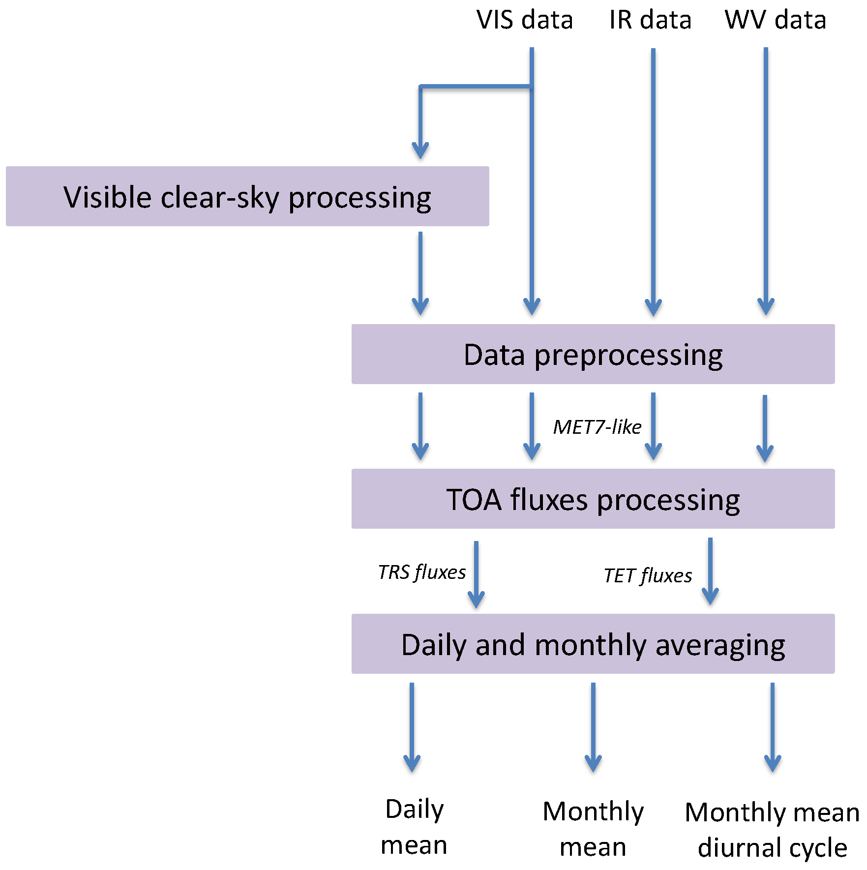
Figure 2.
All-sky VIS image (left) and corresponding CS VIS product (right), expressed in counts, for 10 June 1995 at 12 UTC.
Figure 2.
All-sky VIS image (left) and corresponding CS VIS product (right), expressed in counts, for 10 June 1995 at 12 UTC.

Figure 3.
Overview flowchart for the SW BB radiance to flux conversion.

Figure 4.
Overview flowchart for the LW BB radiance to flux conversion.
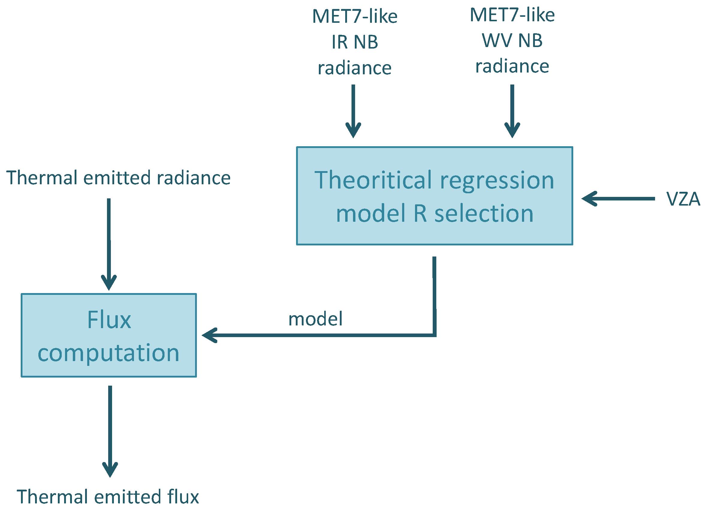
Figure 5.
Averaging strategy: from the hourly integrated data to the daily mean, to the monthly mean diurnal cycle and to the monthly mean product.
Figure 5.
Averaging strategy: from the hourly integrated data to the daily mean, to the monthly mean diurnal cycle and to the monthly mean product.

Figure 6.
Example of the TRS (left) and TET (right) MM products for June 2005 (MSG-1).
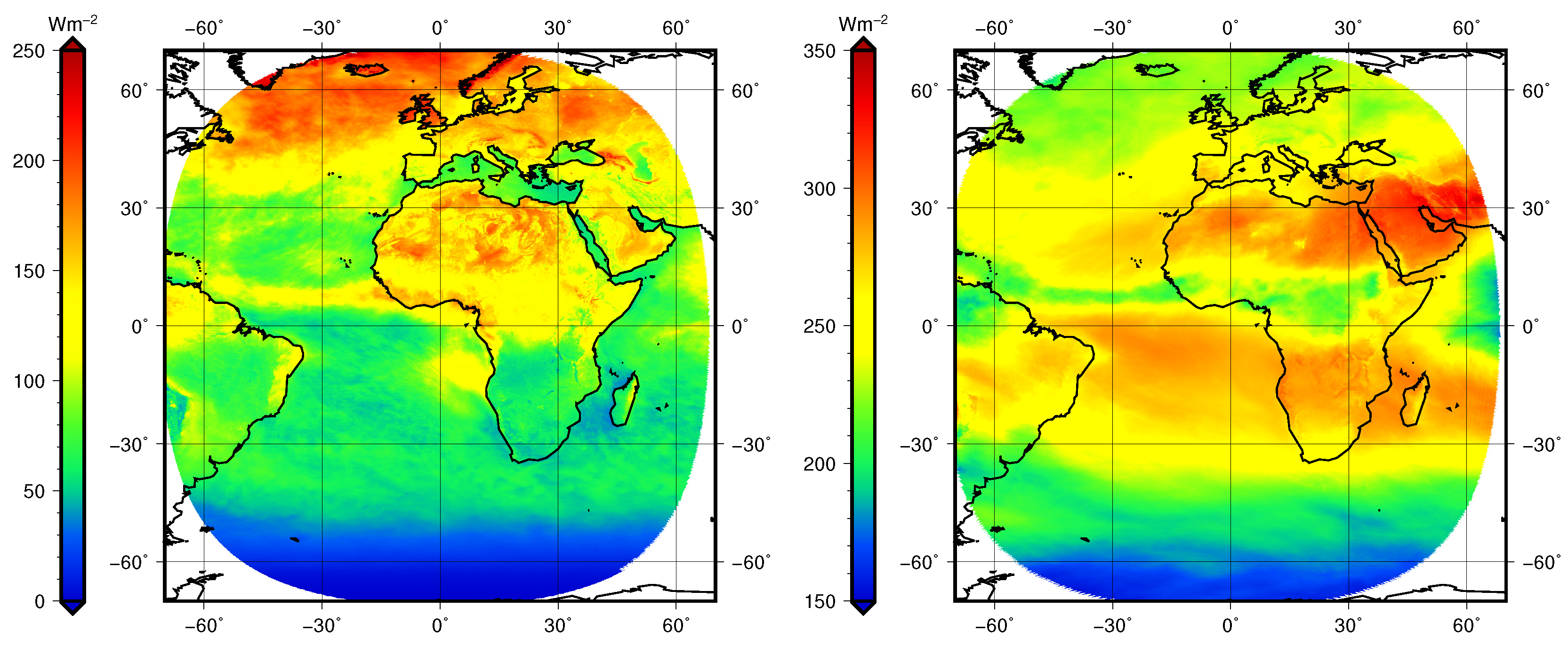
Figure 7.
Example of the TRS (left) and TET (right) DM products for the 1st June 2005 (MSG-1).

Figure 8.
Example of the TRS (left) and TET (right) MMDC products for June 2005 at 08 UTC (MSG-1).

Figure 9.
Time series of the bias between the CM SAF MM and CERES EBAF TRS products. The red dotted line gives the mean bias over the time series while the two black dotted lines at ±2 Wm with respect to the mean bias represents the threshold requirements for stability.
Figure 9.
Time series of the bias between the CM SAF MM and CERES EBAF TRS products. The red dotted line gives the mean bias over the time series while the two black dotted lines at ±2 Wm with respect to the mean bias represents the threshold requirements for stability.
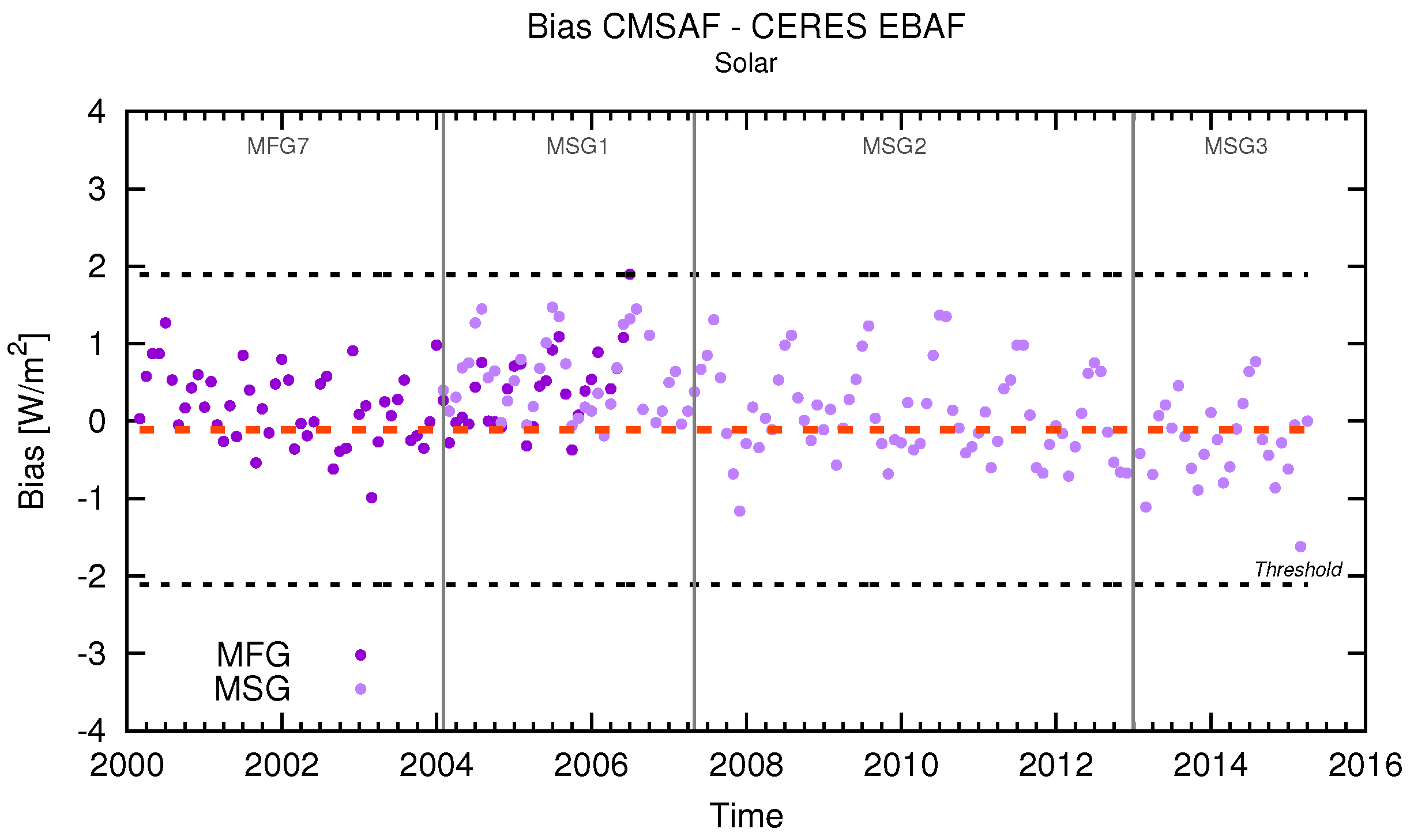
Figure 10.
Time series of the bias between the CM SAF MM and ERBS WFOV-CERES TRS products.
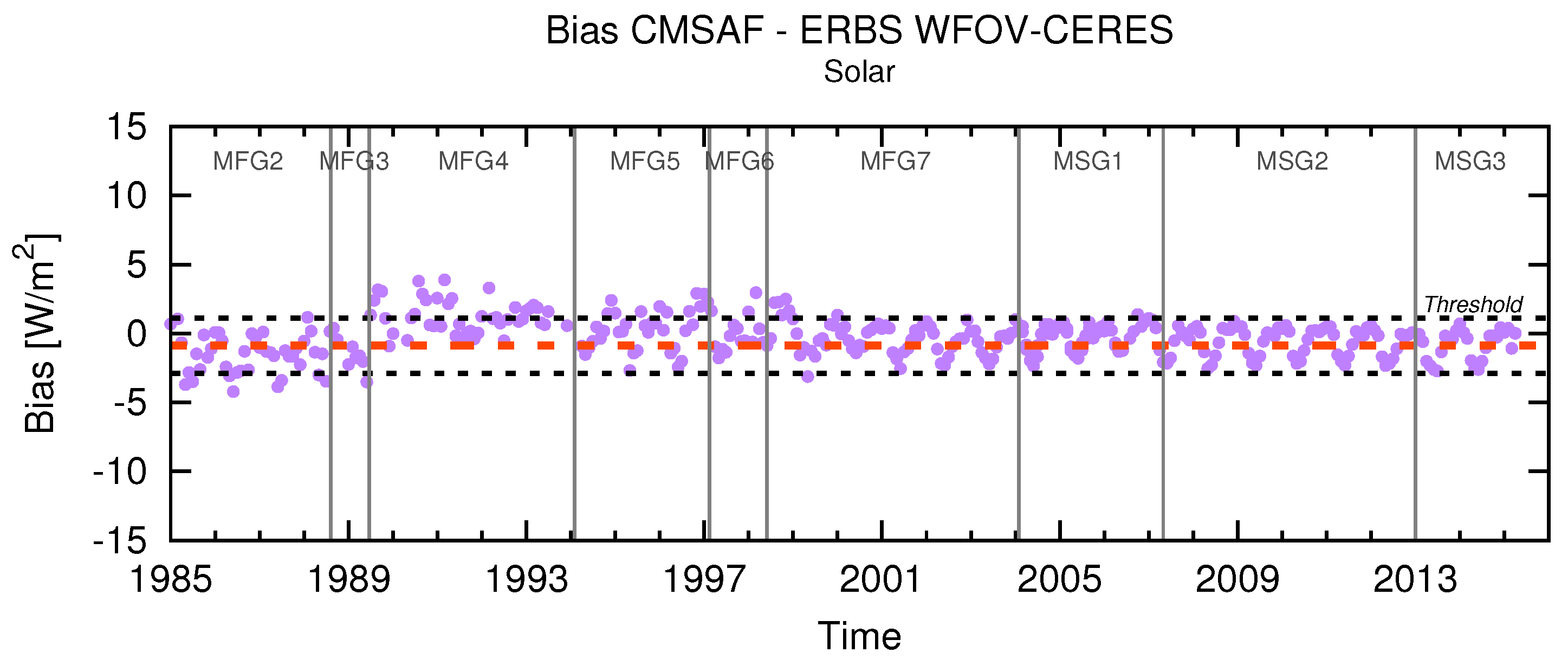
Figure 11.
Time series of the bias between the CM SAF DM and CERES SYN1deg-Day TRS products.

Figure 12.
Time series of the bias between the CM SAF MMDC and CERES SYN1deg-M3Hour TRS products.

Figure 13.
Time series of FOV-averaged clear-sky TRS fluxes, and anomalies, according to various surface types for the 12 UTC repeat cycle. The anomalies are obtained by subtracting the mean clear-sky TRS flux (straight lines) from the time series. An additional shift of −40 Wm, −20 Wm, 0 Wm, 20 Wm, 40 Wm is done to improve the readability of the graph.

Figure 14.
Time series of the RMS difference (bias-corrected) between the CM SAF MM and CERES EBAF TRS products. The red dotted line gives the mean RMS (pre-Aqua period and outliers excepted) over the time series while the black dotted lines give the accuracy requirements (see Section 3).
Figure 14.
Time series of the RMS difference (bias-corrected) between the CM SAF MM and CERES EBAF TRS products. The red dotted line gives the mean RMS (pre-Aqua period and outliers excepted) over the time series while the black dotted lines give the accuracy requirements (see Section 3).

Figure 15.
Time series of the RMS difference (bias-corrected) between the CM SAF DM and CERES SYN1deg-Day TRS products.
Figure 15.
Time series of the RMS difference (bias-corrected) between the CM SAF DM and CERES SYN1deg-Day TRS products.

Figure 16.
Time series of the RMS difference (bias-corrected) between the CM SAF MMDC and CERES SYN1deg-M3Hour TRS products.
Figure 16.
Time series of the RMS difference (bias-corrected) between the CM SAF MMDC and CERES SYN1deg-M3Hour TRS products.

Figure 17.
Time series of the bias between CM SAF MM and CERES EBAF TET products. The red dotted line gives the mean bias over the time series while the two black dotted lines at ±2 Wm with respect to the mean bias represents the threshold requirements for stability.
Figure 17.
Time series of the bias between CM SAF MM and CERES EBAF TET products. The red dotted line gives the mean bias over the time series while the two black dotted lines at ±2 Wm with respect to the mean bias represents the threshold requirements for stability.

Figure 18.
Time series of the bias between the CM SAF TET MM and HIRS OLR CDR-Monthly products. The red dotted line gives the mean bias over the time series (MFG-2 and -3 periods excepted). MFG-2 and -3 data, displayed in red, use the EUMETSAT operational calibration while the GSICS/EUMETSAT recalibration is used for the other satellites.

Figure 19.
Time series of the bias between the CM SAF DM and CERES SYN1deg-Day TET products. The red dotted line gives the mean bias over the time series.
Figure 19.
Time series of the bias between the CM SAF DM and CERES SYN1deg-Day TET products. The red dotted line gives the mean bias over the time series.

Figure 20.
Time series of the bias between the CM SAF TET DM and HIRS OLR CDR-Daily products. The red dotted line gives the mean bias over the time series (MFG-2 and -3 periods excepted).
Figure 20.
Time series of the bias between the CM SAF TET DM and HIRS OLR CDR-Daily products. The red dotted line gives the mean bias over the time series (MFG-2 and -3 periods excepted).
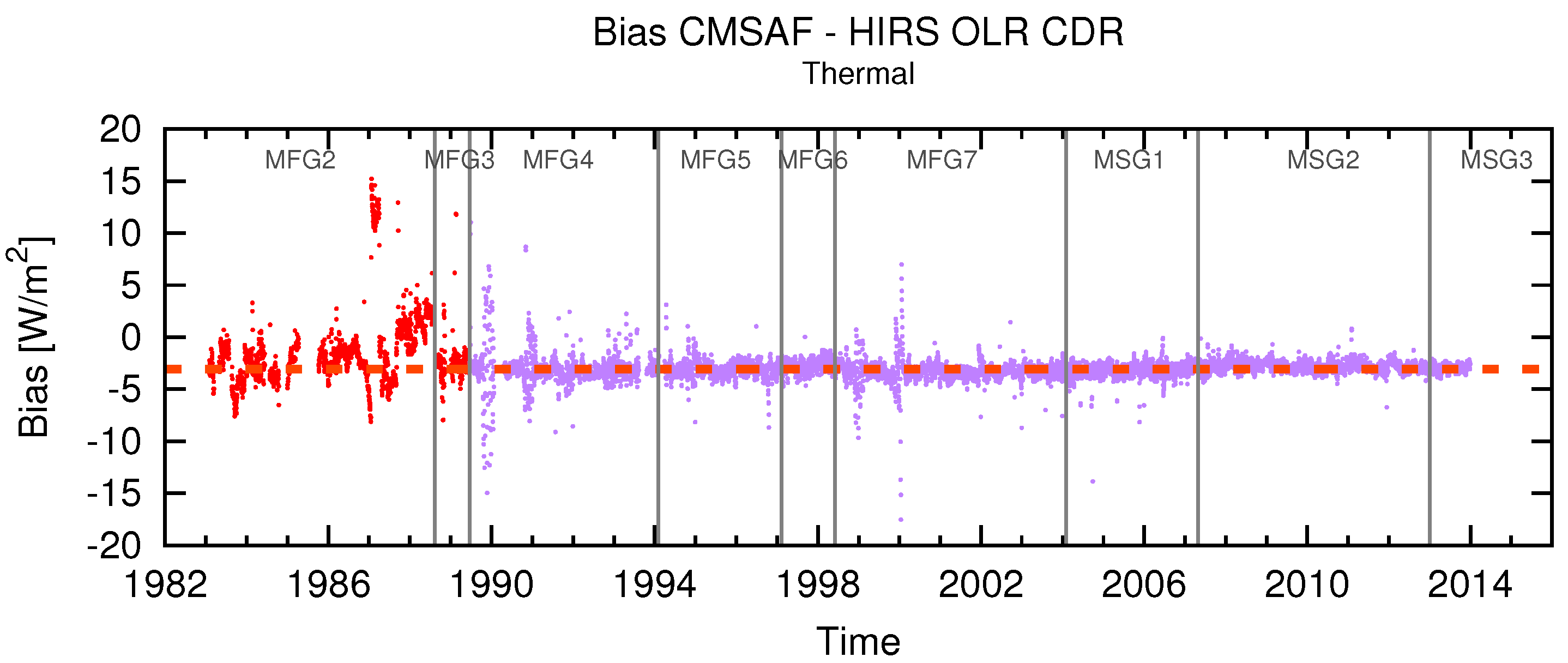
Figure 21.
Time series of the bias between the CM SAF MMDC and CERES SYN1deg-M3Hour TET products.
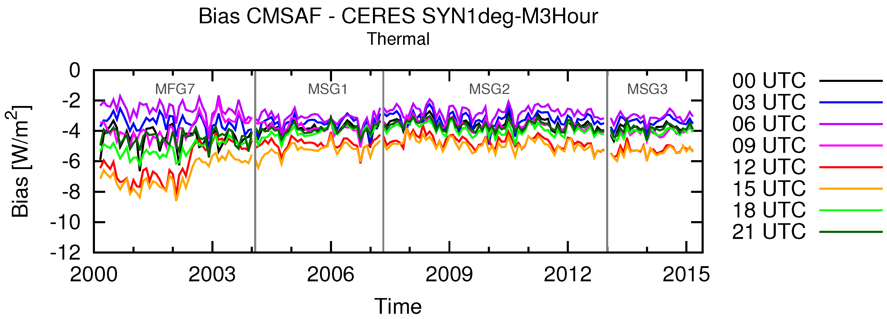
Figure 22.
Time series of FOV-averaged TET fluxes, and anomalies, according to various surface types for the 12 UTC repeat cycle. The anomalies are obtained by subtracting the mean TET flux (straight lines) from the time series. An additional shift of −40 Wm, −20 Wm, 0 Wm, 20 Wm, 40 Wm is done to improve the readability of the graph.

Figure 23.
Time series of the RMS difference (bias-corrected) between the CM SAF MM and CERES EBAF TET products. The red dotted line gives the mean RMS over the time series while the black dotted lines give the accuracy requirements (see Section 3).
Figure 23.
Time series of the RMS difference (bias-corrected) between the CM SAF MM and CERES EBAF TET products. The red dotted line gives the mean RMS over the time series while the black dotted lines give the accuracy requirements (see Section 3).

Figure 24.
Time series of the RMS difference (bias-corrected) between CM SAF DM and CERES SYN1deg-Day TET products. The red dotted line gives the mean RMS over the time series (pre-Aqua period excepted).
Figure 24.
Time series of the RMS difference (bias-corrected) between CM SAF DM and CERES SYN1deg-Day TET products. The red dotted line gives the mean RMS over the time series (pre-Aqua period excepted).
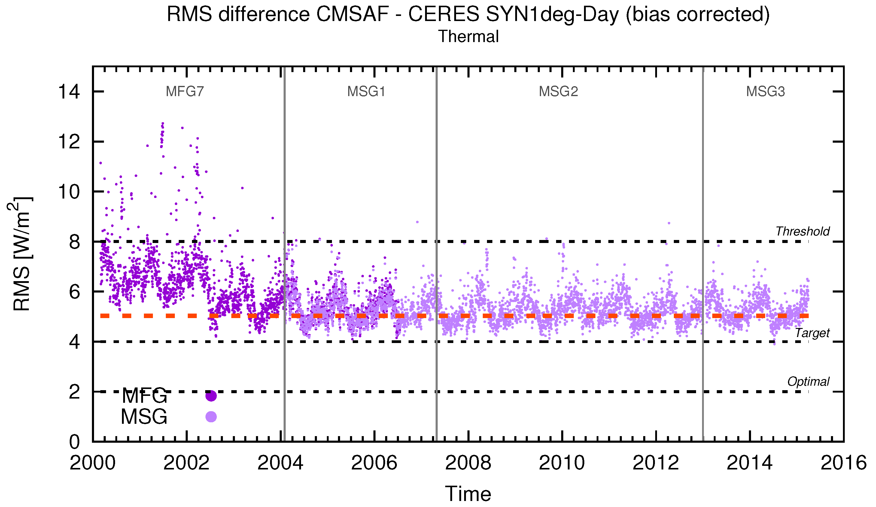
Figure 25.
Time series of the RMS difference (bias-corrected) between CM SAF DM and HIRS OLR CDR-Daily products. The red dotted line gives the mean RMS over the time series (MFG-2 and -3 periods excepted).
Figure 25.
Time series of the RMS difference (bias-corrected) between CM SAF DM and HIRS OLR CDR-Daily products. The red dotted line gives the mean RMS over the time series (MFG-2 and -3 periods excepted).

Figure 26.
Time series of the RMS difference (bias-corrected) between the CM SAF MMDC and CERES SYN1deg-M3Hour TET products.
Figure 26.
Time series of the RMS difference (bias-corrected) between the CM SAF MMDC and CERES SYN1deg-M3Hour TET products.


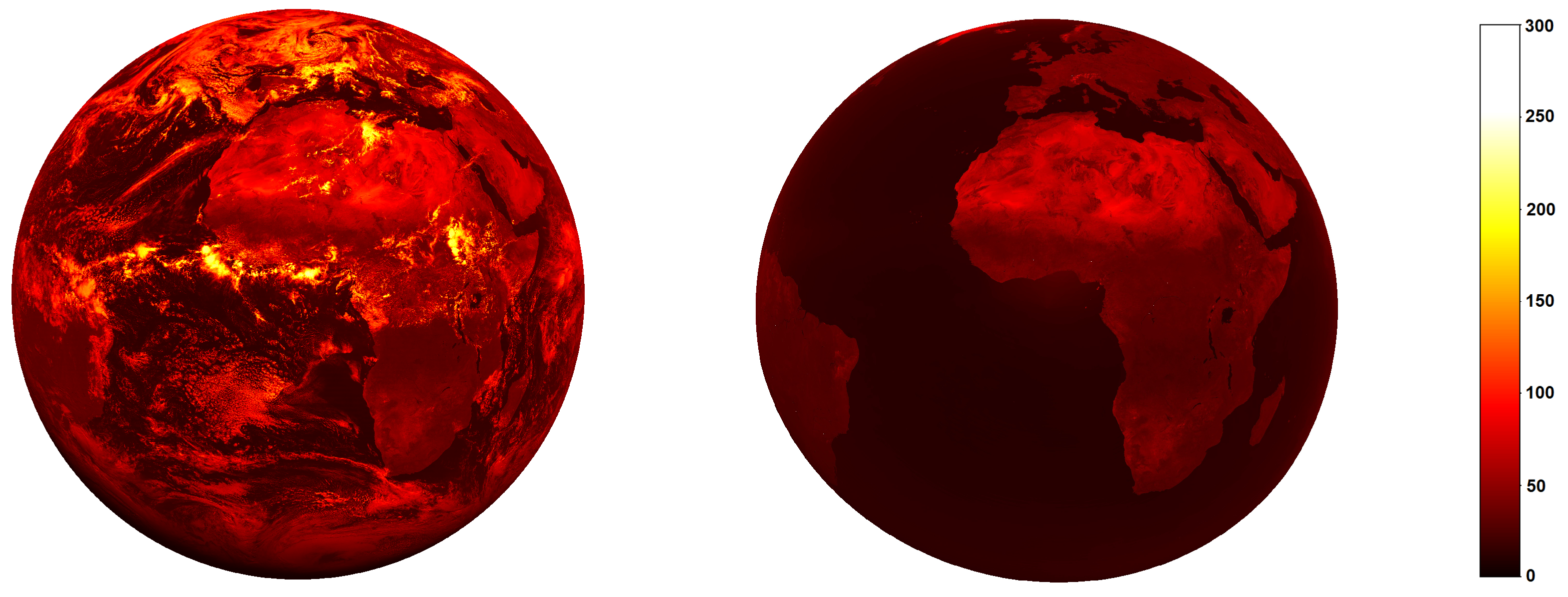
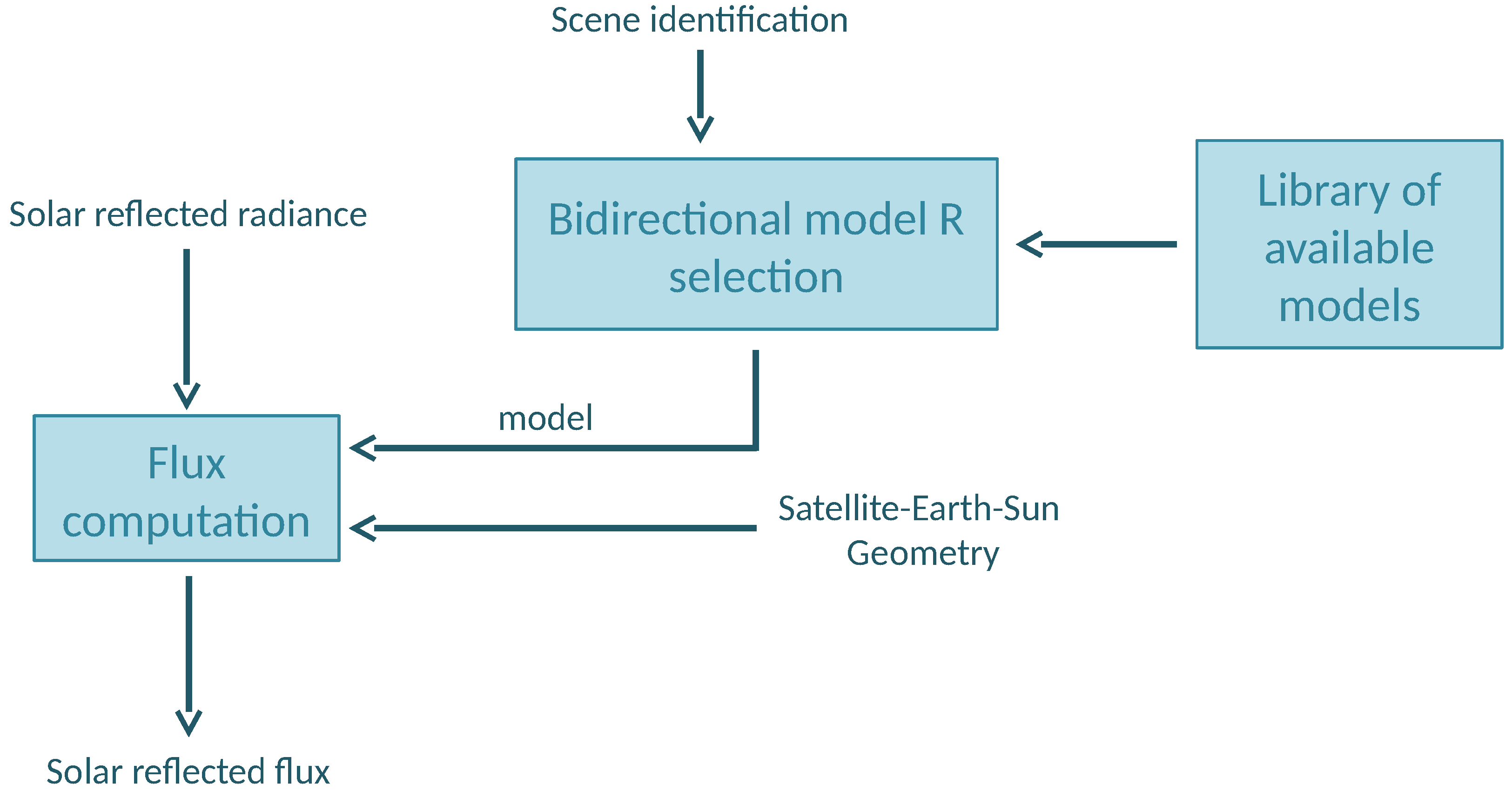
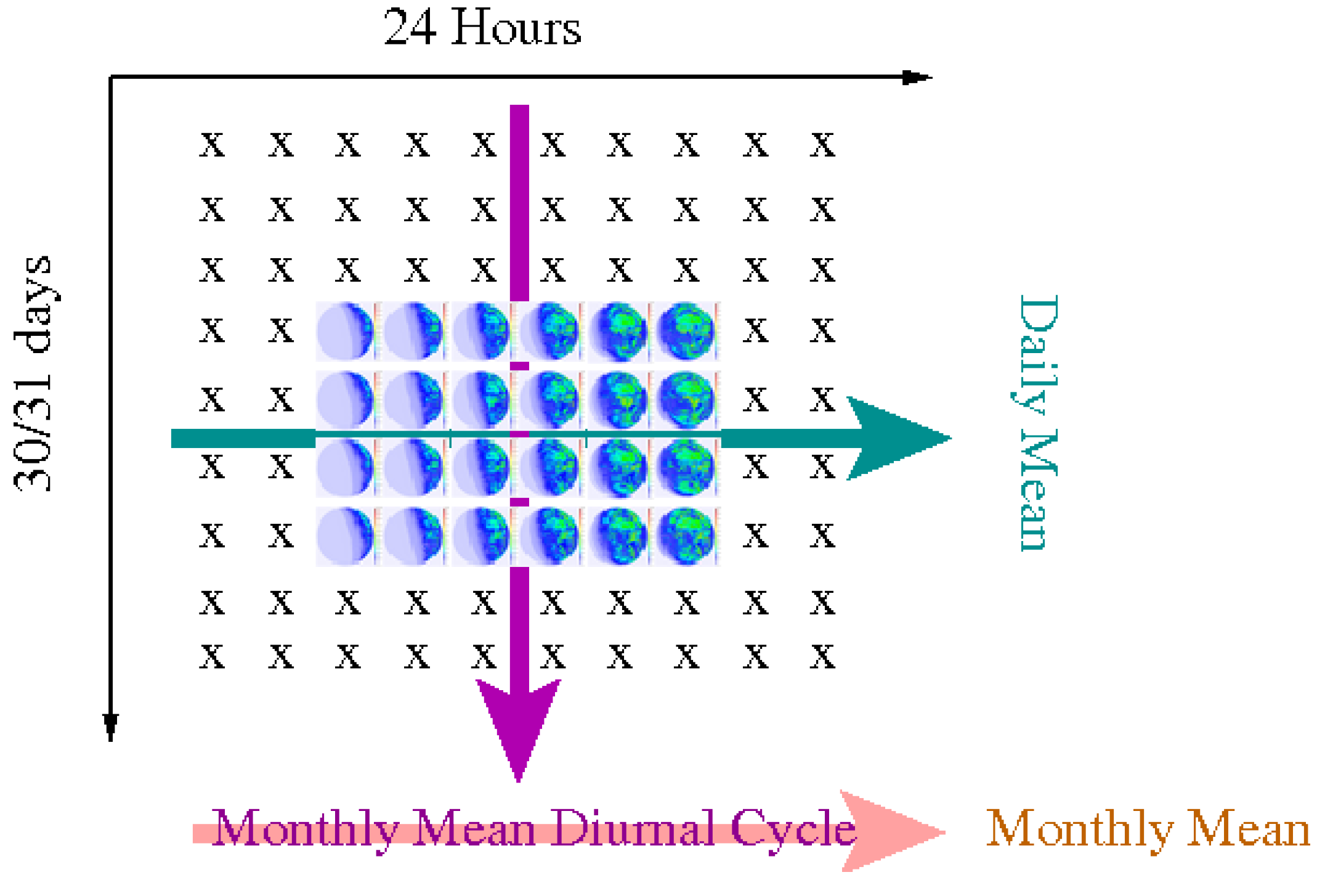
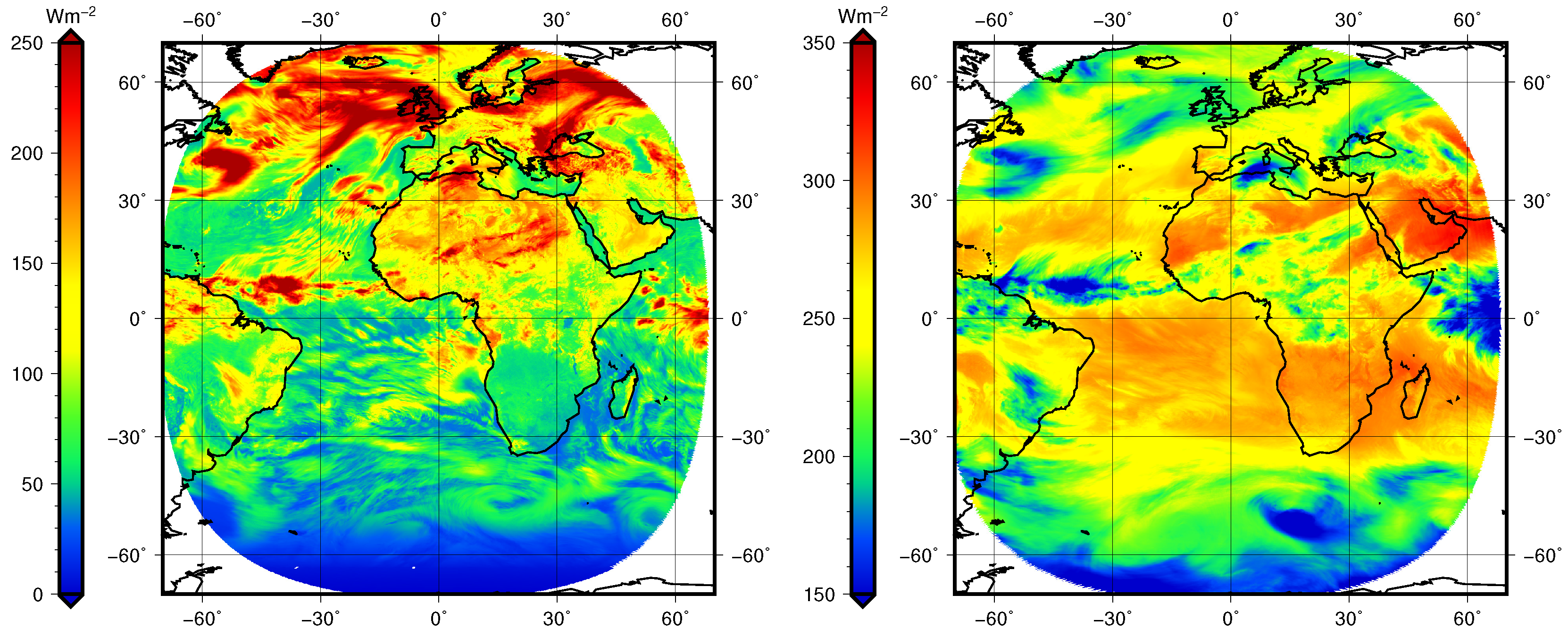
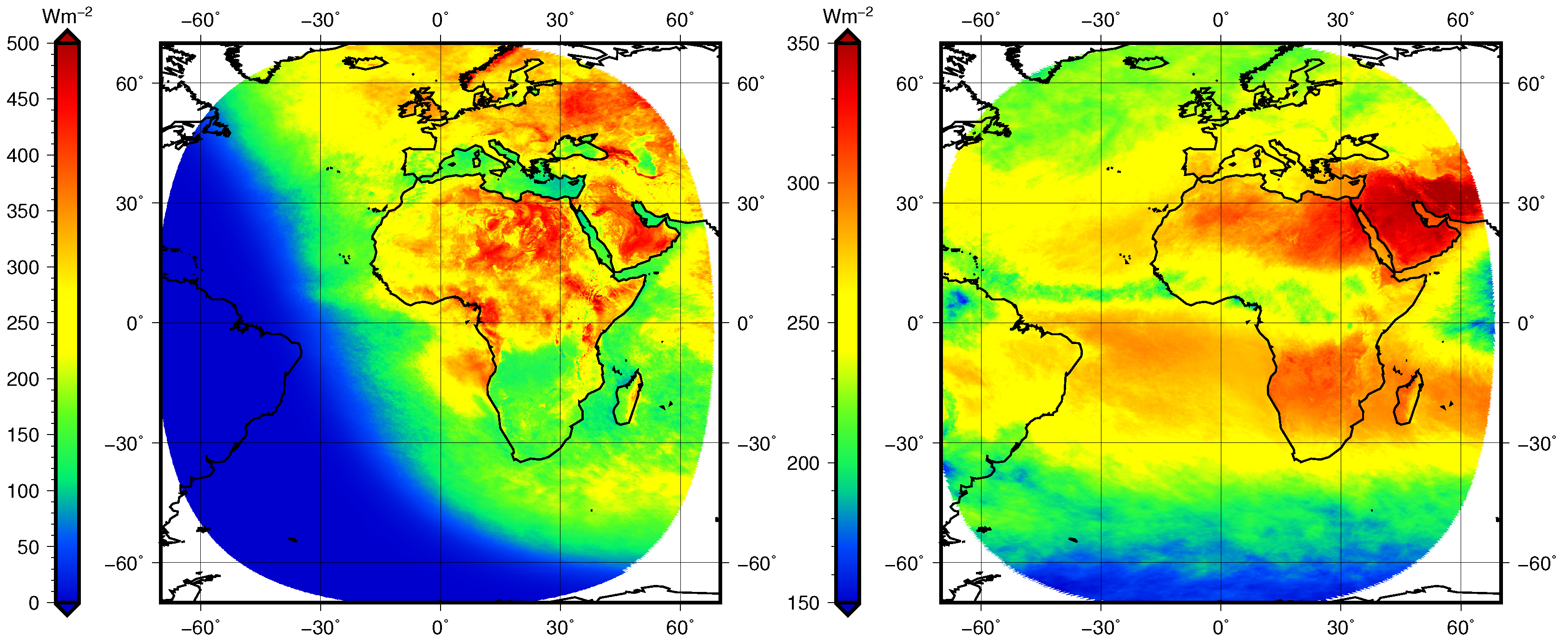
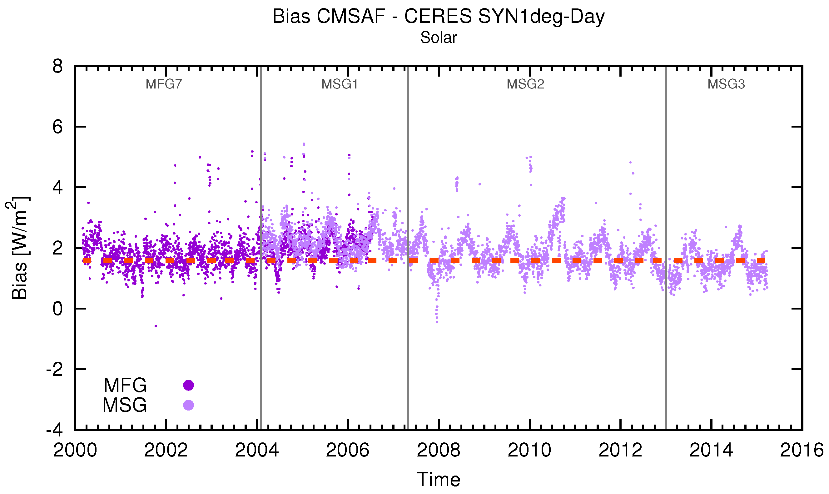
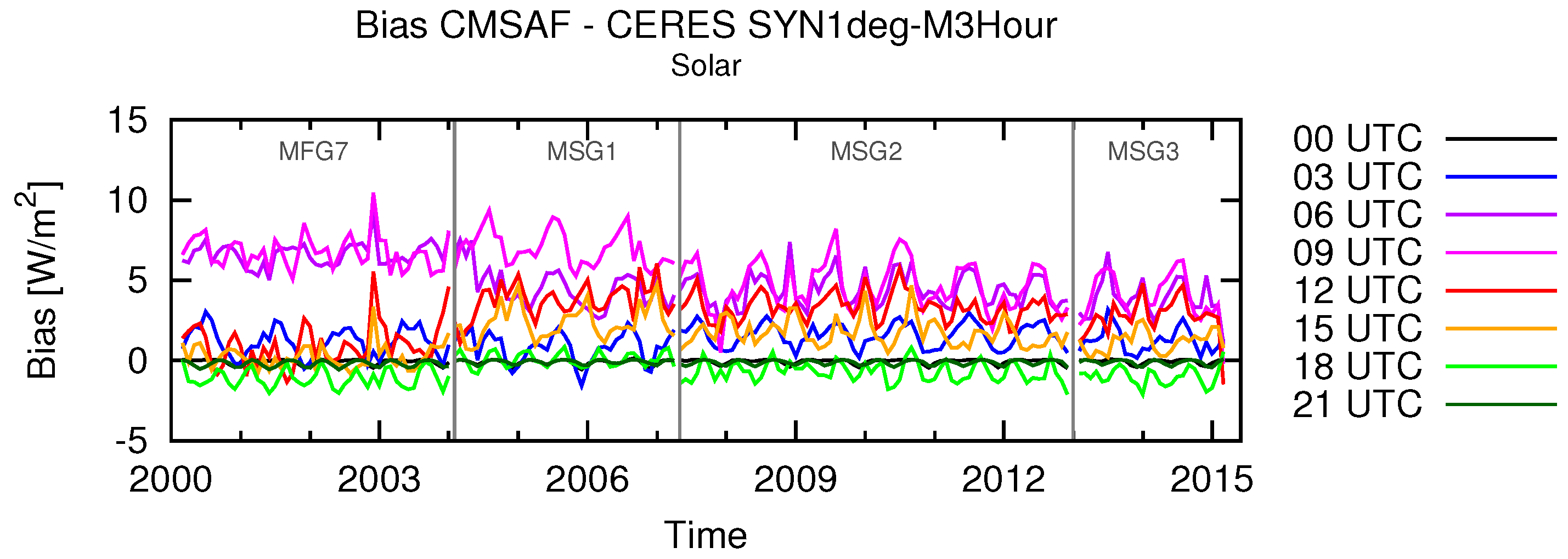
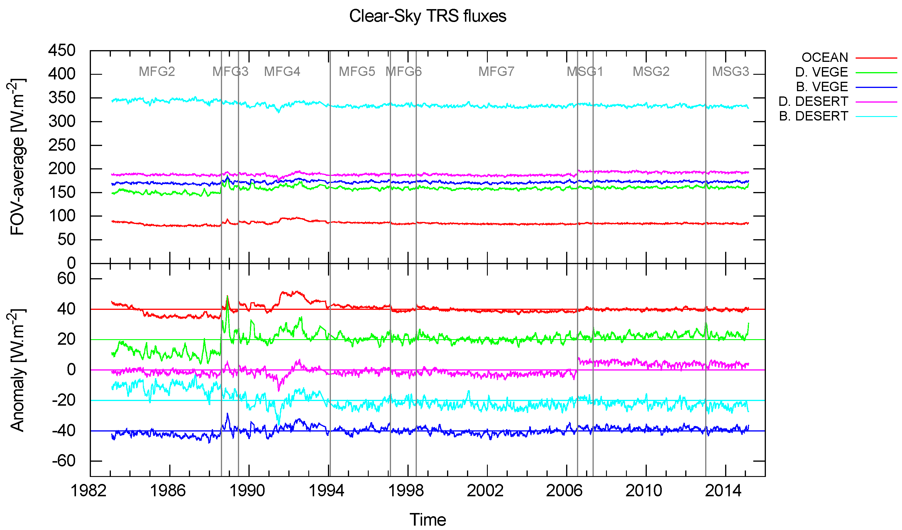
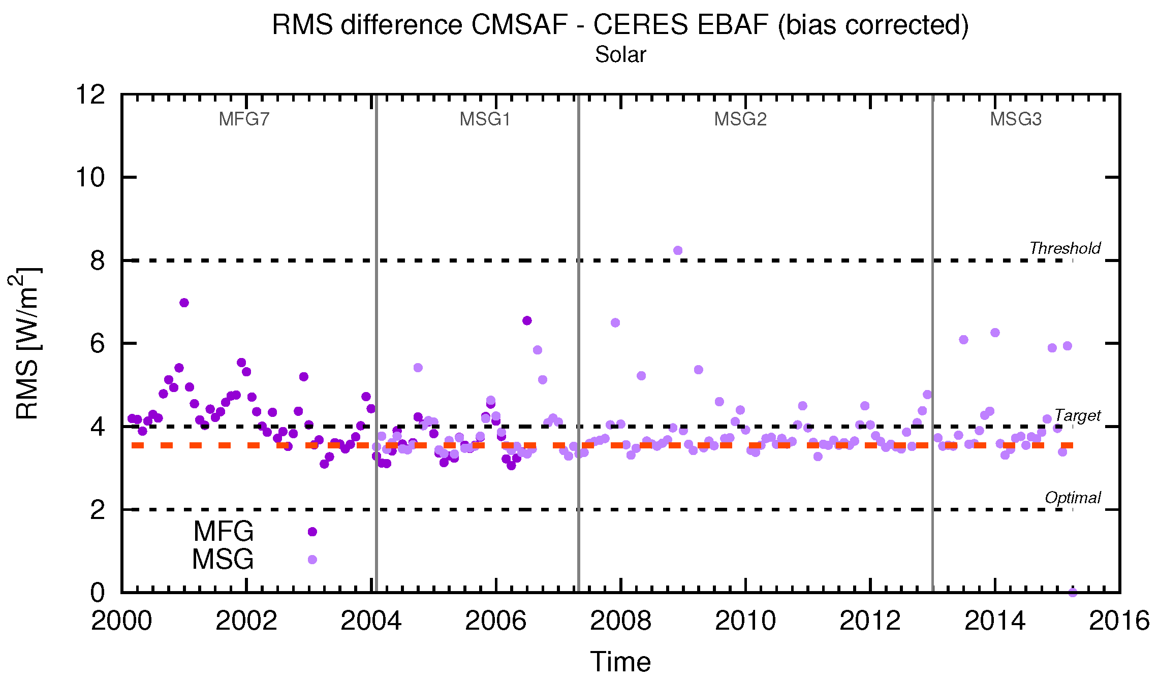
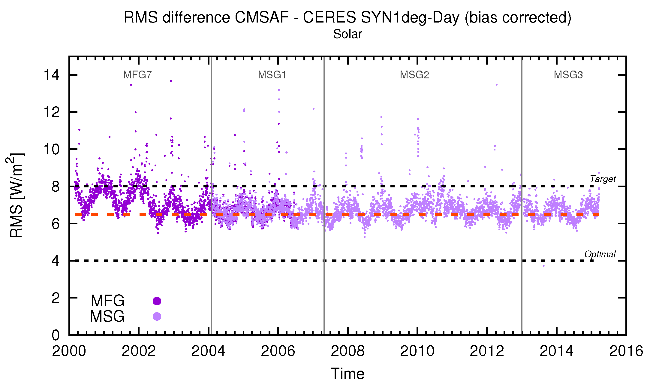
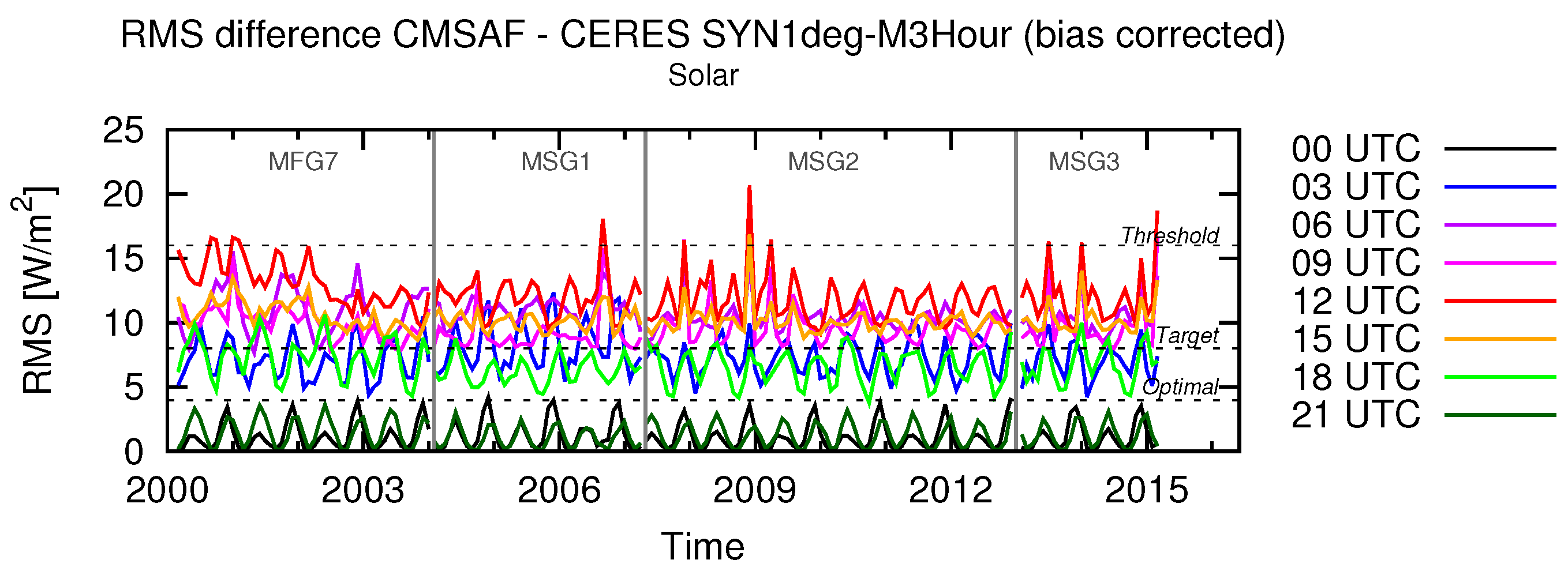
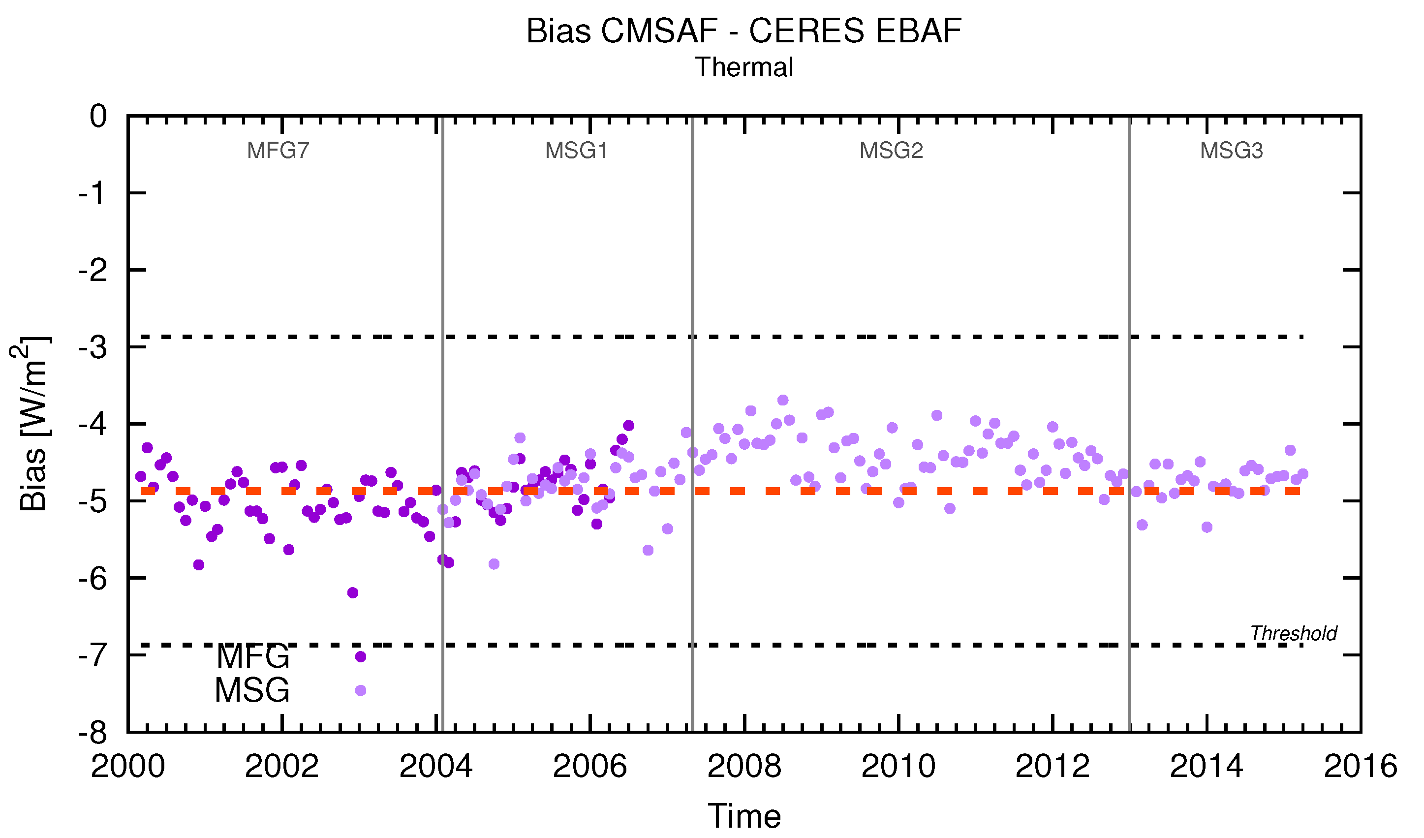
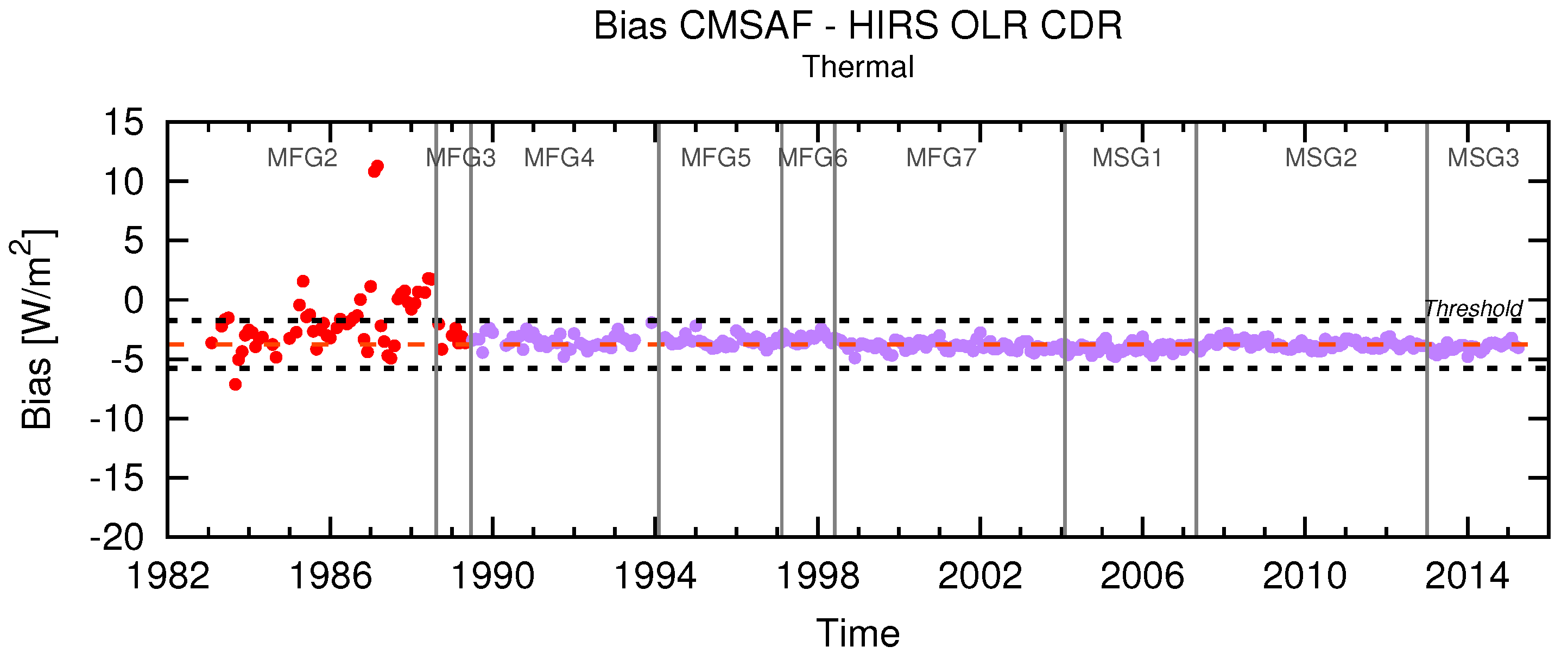
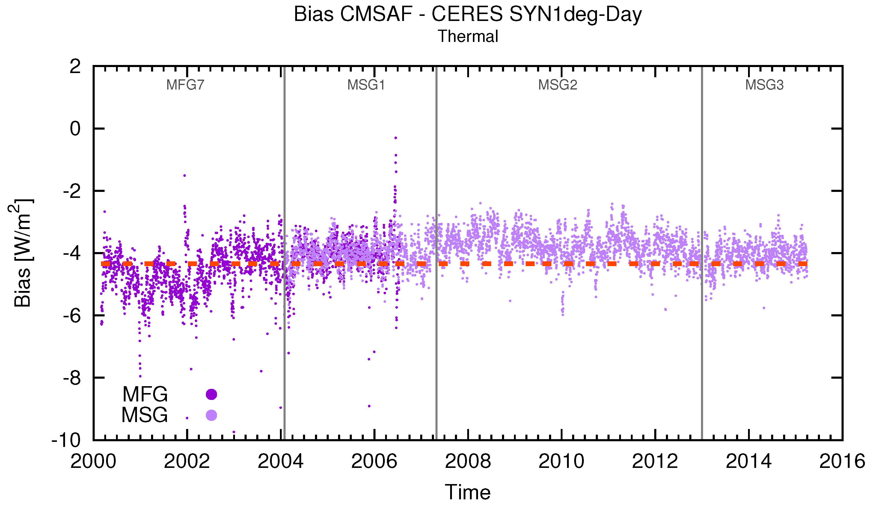
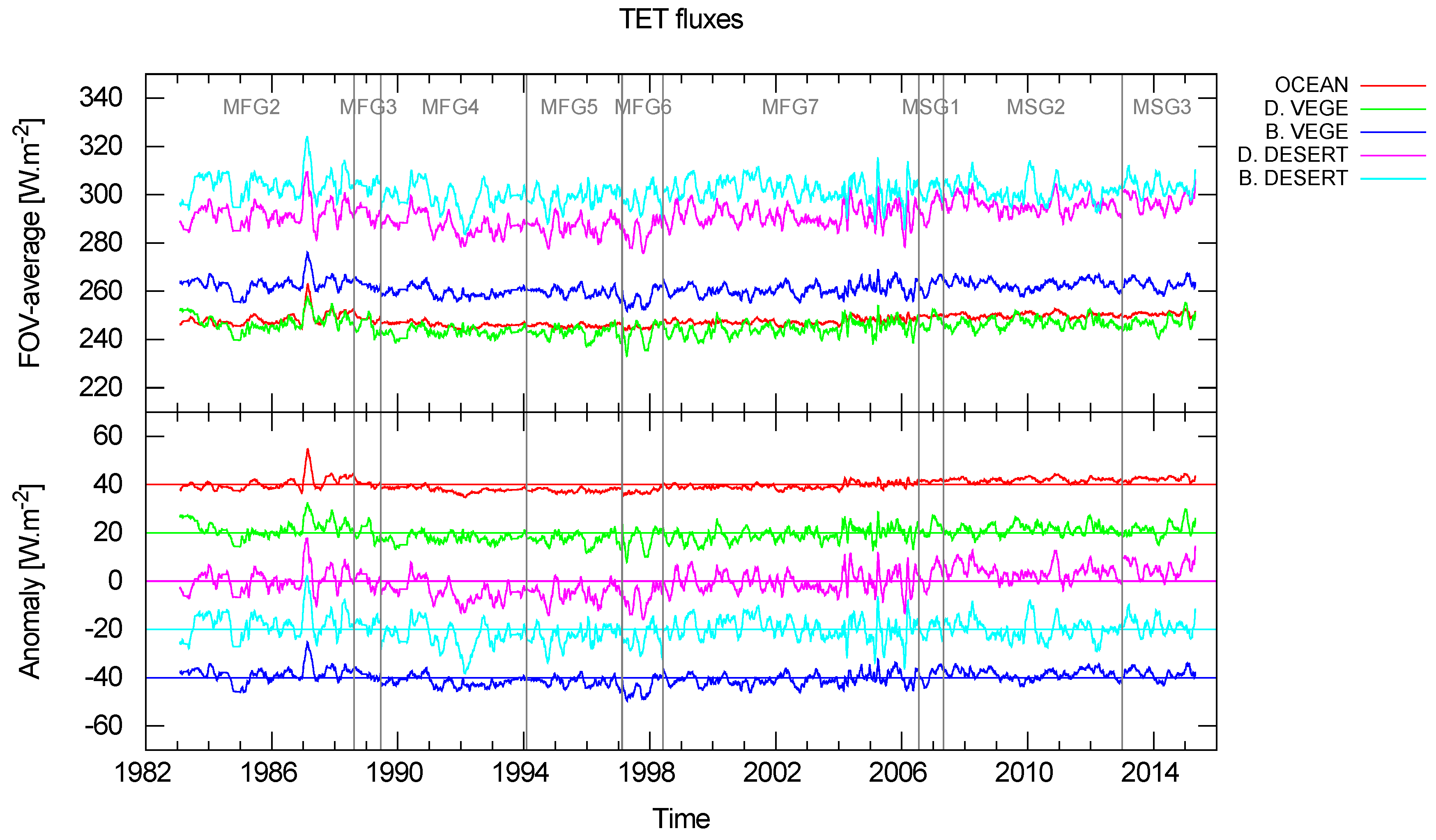
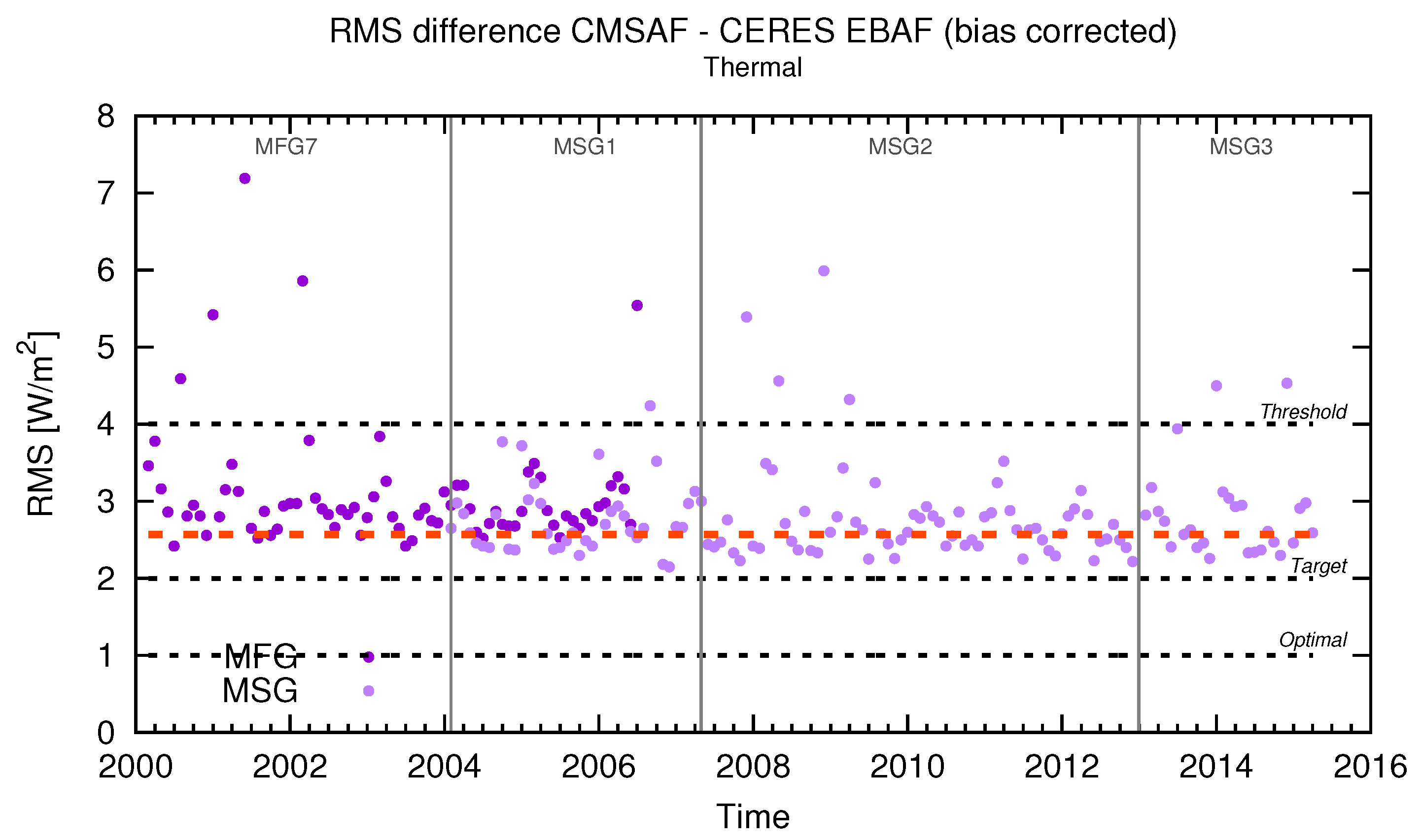
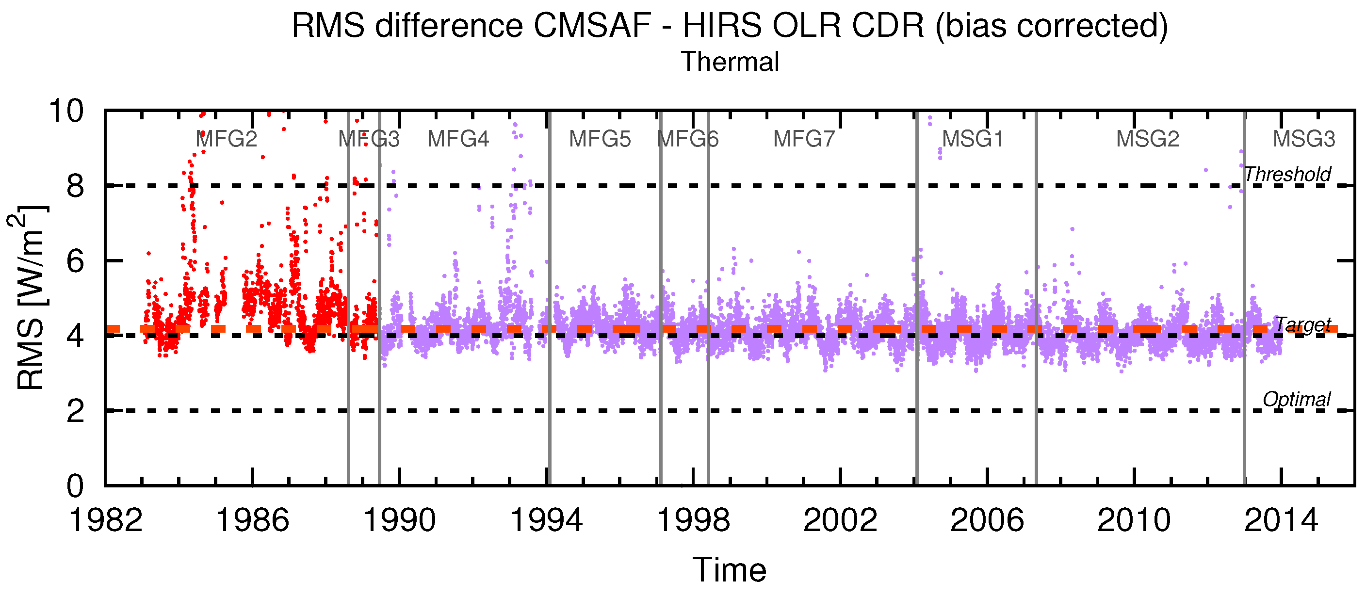
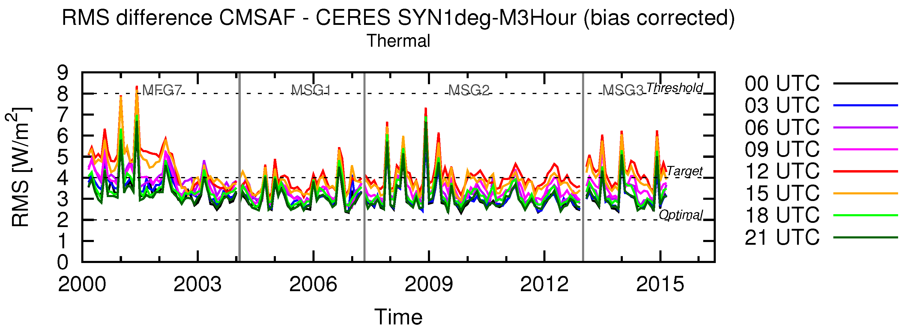
Table 1.
Launch date, nominal longitude and data period used for the Meteosat satellites.
| Satellite | Launch Date | Used Data Period | Nominal Longitude | |
|---|---|---|---|---|
| MFG | Meteosat-1 (MFG-1) | 23/11/1977 | - | 0 |
| Meteosat-2 (MFG-2) | 19/06/1981 | 01/02/1983–11/08/1988 | 0 | |
| Meteosat-3 (MFG-3) | 15/06/1988 | 11/08/1988–19/06/1989 | 0 | |
| Meteosat-4 (MFG-4) | 06/03/1989 | 19/06/1989–04/02/1994 | 0 | |
| Meteosat-5 (MFG-5) | 02/03/1991 | 04/02/1994–13/02/1997 | 0 | |
| Meteosat-6 (MFG-6) | 19/11/1993 | 13/02/1997–03/06/1998 | 0 | |
| Meteosat-7 (MFG-7) | 02/09/1997 | 03/06/1998–31/01/2004 | 0 | |
| MSG | Meteosat-8 (MSG-1) | 28/08/2002 | 01/02/2004–30/04/2007 | 3.5 West |
| Meteosat-9 (MSG-2) | 21/12/2005 | 01/05/2007–31/12/2012 | 0 | |
| Meteosat-10 (MSG-3) | 05/07/2012 | 22/01/2013–30/04/2015 | 0 | |
| Meteosat-11 (MSG-4) | 15/07/2015 | - | 0 | |
Table 2.
Stability requirements for the MVIRI/SEVIRI data record.
| Products | Threshold | Target | Optimal |
|---|---|---|---|
| TRS MM | 4 Wm/decade | 0.6 Wm/decade | 0.3 Wm/decade |
| TET MM | 4 Wm/decade | 0.6 Wm/decade | 0.3 Wm/decade |
Table 3.
Accuracy requirements for the MVIRI/SEVIRI data record.
| Products | Threshold | Target | Optimal | |
|---|---|---|---|---|
| TRS | MM | 8 Wm | 4 Wm | 2 Wm |
| DM | 16 Wm | 8 Wm | 4 Wm | |
| MMDC | 16 Wm | 8 Wm | 4 Wm | |
| TET | MM | 4 Wm | 2 Wm | 1 Wm |
| DM | 8 Wm | 4 Wm | 2 Wm | |
| MMDC | 8 Wm | 4 Wm | 2 Wm | |
Table 4.
Calibration methods used for the MVIRI/SEVIRI data record.
| Instrument | Solar Channels (TRS) | Thermal Channels (TET) |
|---|---|---|
| MVIRI | SEVIRI Solar Channel Calibration [15] | MFG-2 and -3: operational calibration |
| MFG-4 to -7: GSICS/EUMETSAT recalibration using HIRS (R. Stöckli and A. Tetzlaff, pers. comm.) | ||
| SEVIRI | KNMI SEVIRI recalibration [16] | EUMETSAT operational calibration (available in the prologue of the L1.5 Meteosat images) |
Table 5.
Main characteristics of the data records used for evaluation purpose.
| Source | Version | Variable | Temporal | Spatial | Period | References |
|---|---|---|---|---|---|---|
| Resolution | Resolution | |||||
| CERES EBAF | 2.8 | TRS | MM | 1 × 1 | March 2000 | [33,34] |
| TET | onward | |||||
| CERES SYN1deg-Day | 3A | TRS | DM | 1 × 1 | March 2000 | [35,36] |
| TET | onward | |||||
| CERES SYN1deg-M3 Hour | 3A | TRS | MMDC | 1 × 1 | March 2000 | [35,36] |
| TET | (3-hourly) | onward | ||||
| HIRS OLR CDR | 2.7 1 | TET | MM | 2.5 × 2.5 | January 1979 | pers. comm. |
| Monthly | onward | H.-T. Lee | ||||
| HIRS OLR CDR | 1.2 | TET | DM | 1 × 1 | January 1979 to | [37,38] |
| Daily | December 2013 | |||||
| ERBS WFOV-CERES | 2 | TRS | MM | 0.7 × 0.7 | January 1985 to | [39,40,41] |
| (DEEP-C) | TET | May 2015 | ||||
| ISCCP FD | - | TRS | MM | 2.5 × 2.5 | July 1983 to | [42] |
| TET | MMDC | December 2004 |
The current official release is version 2.2. However, this version is known to have artificial trends and discontinuities mainly caused by inconsistent regression models used for the OLR retrieval across the HIRS instruments (pers. comm. H.-T. Lee). Version 2.7 uses new sets of regression models which improve the accuracy of inter-satellite calibration and is expected to replace version 2.2.
Table 6.
Errors and additional uncertainties affecting the monthly mean (MM), daily mean (DM) and monthly mean diurnal cycle (MMDC) products.
Table 6.
Errors and additional uncertainties affecting the monthly mean (MM), daily mean (DM) and monthly mean diurnal cycle (MMDC) products.
| MM | DM | MMDC | ||||
|---|---|---|---|---|---|---|
| Error/Uncertainty | TRS | TET | TRS | TET | TRS | TET |
| Sources | (Midday) (R.3) | |||||
| Stability error | Stability of all the products better than 4 Wm (max-min) except for the TET during a given period in 1987 (MFG-2) (R.4) | |||||
| Processing error | 3.6 Wm | 2.6 Wm | 6.5 Wm | 4.2 Wm | 11.0 Wm | 3.5 Wm |
| (at 1 std. dev.) | ||||||
| Additional uncertainty due to missing input data | 0.3 Wm/day | 0.2 Wm/day | 0.5 Wm | 0.3 Wm | 0.7 Wm/day | 0.3 Wm/day |
| (R.1) (R.2) | ||||||
© 2017 by the authors. Licensee MDPI, Basel, Switzerland. This article is an open access article distributed under the terms and conditions of the Creative Commons Attribution (CC BY) license (http://creativecommons.org/licenses/by/4.0/).
Share and Cite
MDPI and ACS Style
Urbain, M.; Clerbaux, N.; Ipe, A.; Tornow, F.; Hollmann, R.; Baudrez, E.; Velazquez Blazquez, A.; Moreels, J. The CM SAF TOA Radiation Data Record Using MVIRI and SEVIRI. Remote Sens. 2017, 9, 466. https://doi.org/10.3390/rs9050466
AMA Style
Urbain M, Clerbaux N, Ipe A, Tornow F, Hollmann R, Baudrez E, Velazquez Blazquez A, Moreels J. The CM SAF TOA Radiation Data Record Using MVIRI and SEVIRI. Remote Sensing. 2017; 9(5):466. https://doi.org/10.3390/rs9050466
Chicago/Turabian StyleUrbain, Manon, Nicolas Clerbaux, Alessandro Ipe, Florian Tornow, Rainer Hollmann, Edward Baudrez, Almudena Velazquez Blazquez, and Johan Moreels. 2017. "The CM SAF TOA Radiation Data Record Using MVIRI and SEVIRI" Remote Sensing 9, no. 5: 466. https://doi.org/10.3390/rs9050466
Note that from the first issue of 2016, this journal uses article numbers instead of page numbers. See further details here.