1. Introduction and State of the Art
GNSS (Global Navigation Satellite System) signals reflected from the surface of the sea can be used to infer its physical properties, such as the sea-surface roughness [
1] and altimetry [
2]. This measurement concept is known as GNSS Reflectometry (GNSS-R) or as PAssive Reflectometry and Interferometry System (PARIS). In a multistatic configuration with many GNSS transmitters, one single receiver can observe multiple reflection points simultaneously, providing a synoptic view of the sea surface. Despite its limited altimetric precision compared to conventional radar altimeters, GNSS-R is a measurement concept for synoptic mesoscale altimetry that has been taken into consideration by the European Space Agency [
3,
4].
Several GNSS-R signal processing techniques have been proposed, and interferometric GNSS-R (iGNSS-R) [
3] is among the most promising for altimetric applications as it yields an enhanced ranging precision. This technique consists of acquiring the direct line-of-sight and the sea-surface reflected GNSS transmitter signals from an airborne or space-borne platform and computing the delay and Doppler compensated cross-correlation function between both signals. From the resulting waveform, the altimetric delay is estimated, e.g., [
5]. By using the direct cross-correlation between the direct and reflected signals, the whole bandwidth of the GNSS signals is exploited, including those of the non-public signals. However, the required separability between different GNSS transmitter signals has to be achieved by Doppler filtering and by using narrow beam antennas at the receiver pointing towards the transmitter and the specular reflection point. This is especially the case in airborne platforms, where the Doppler differences between different reflected signals are too close to be used as a means of separation. In contrast, the clean-replica correlation technique [
6] uses code-correlation to achieve separability between different transmitters, and can be used with non-directive antennas. However, it suffers from a very reduced bandwidth since it is limited to civilian signals.
In 2011, we first demonstrated the iGNSS-R concept for altimetry on board an aircraft by using two fixed, high-gain zenith and nadir pointing antennas, and by selecting a proper acquisition time window with a single GPS (Global Positioning System) transmitter at high elevation [
7,
8]. In spite of the success, this scheme only allowed us to obtain single iGNSS-R observations at a time.
To demonstrate synoptic altimetric measurements with the iGNSS-R technique, we have developed the Software PARIS Interferometric Receiver (SPIR). This instrument collects raw data from all individual elements of two antenna arrays of eight elements at a high rate (320 MBytes/s) and saves them to solid state disks, and all data samples are recorded with precise time-tagging with respect to UTC (Coordinated Universal Time) time. Data processing is completed by an off-line software signal processor. This approach allows for pointing of the antennas in post-processing, thus enabling the possibility of selecting different GNSS signals at the same time. It is also possible to reprocess exactly the same data using different algorithms to compare their performance. Previous work in this line has been reported in [
9,
10].
This paper first describes the instrument hardware and its software processor. Then, it shows instrument validation measurements for significant subsystems and presents a selection of observables (waveforms) using the clean-replica and interferometric techniques which were acquired during an airborne campaign over the Baltic Sea. The paper ends with some concluding remarks.
2. Instrument Description
2.1. Architecture
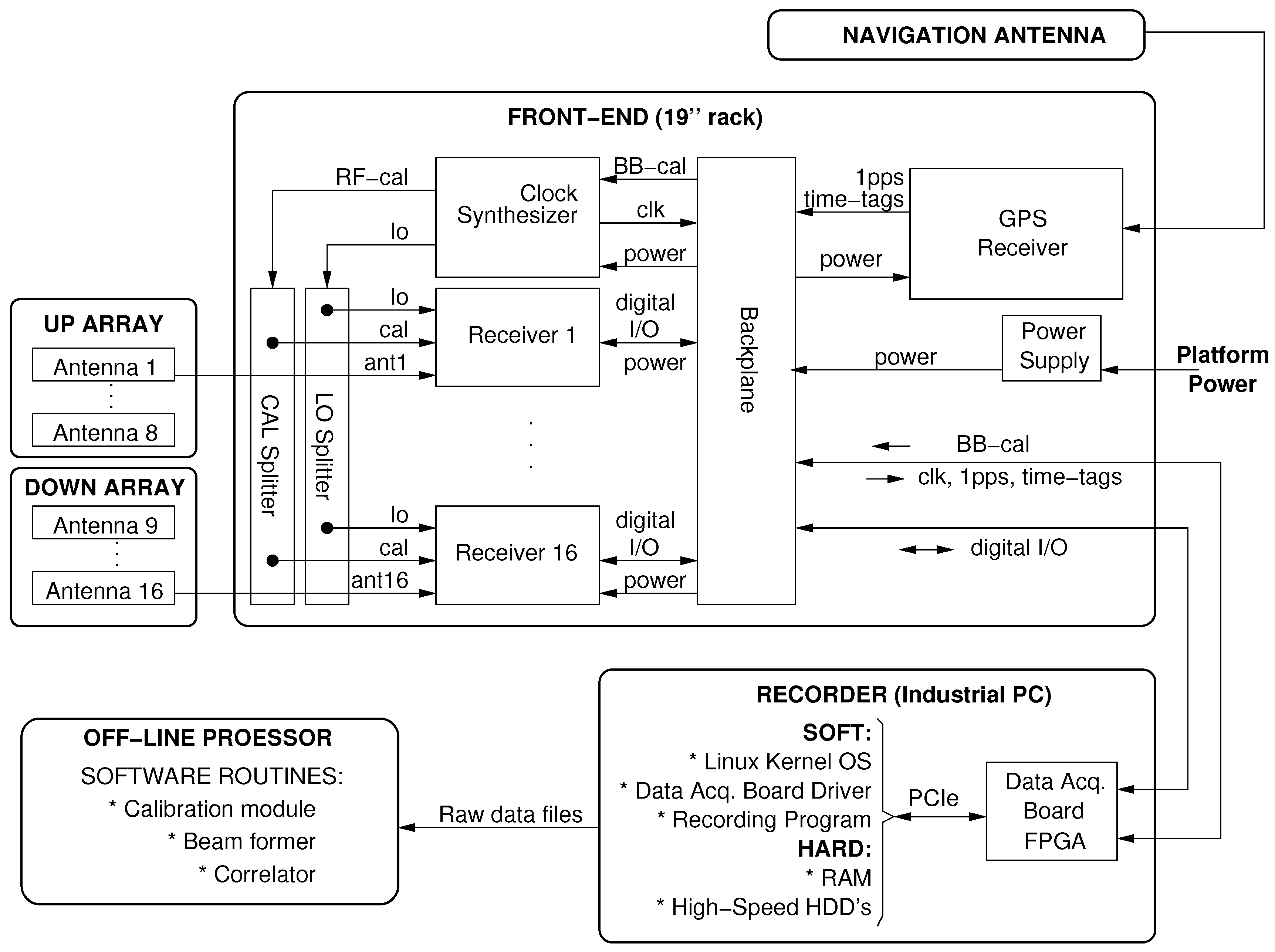
A block diagram of the SPIR instrument is shown in
Figure 1. It features two arrays, up- and down-looking, of eight elements each. The polarization of the antenna elements is RHCP (Right Hand Circular Polarization) and LHCP (Left Hand Circular Polarization) for the up and down-looking arrays, respectively. The signals delivered by these antenna elements are fed into 16 identical radio-frequency (RF) receivers that down-convert the signals to an intermediate frequency (IF). The in-phase and quadrature components are digitized with one bit per sample and are sampled at a rate of 80 Msamples/s.
A clock synthesizer board generates the system reference frequency, from which the sampling clock, the local oscillator and the calibration signals are derived. Sixteen replicas of the local oscillator are delivered to all RF front-ends by using a 1:16 passive splitter. An identical splitter is used to deliver the calibration signal to all receivers.
The quantized and sampled signals (16×2 I/Q bits) are then injected into the control and recording system, which consists of an industrial computer with a Field Programmable Gate Array (FPGA) board connected to one of its Peripheral Component Interconnect Express (PCIe) slots. This FPGA collects and buffers the sampled signals to write them to an array of disks. In addition to the raw data, it also records ancillary data and the instrument configuration status (reference frequency, local oscillator, selected band, calibration parameters, and time-tagging information). The control and recording subsystem also retrieves GPS time and position information from a standard GPS receiver, as well as a one pulse per second (PPS) signal that is used to synchronize the recording of the data to UTC time.
The instrument is configured through a program running on the computer, which is also used to start and stop the recording. Once the data have been recorded, they are processed by a dedicated software processor (see
Section 2.6).
2.2. RF Receivers
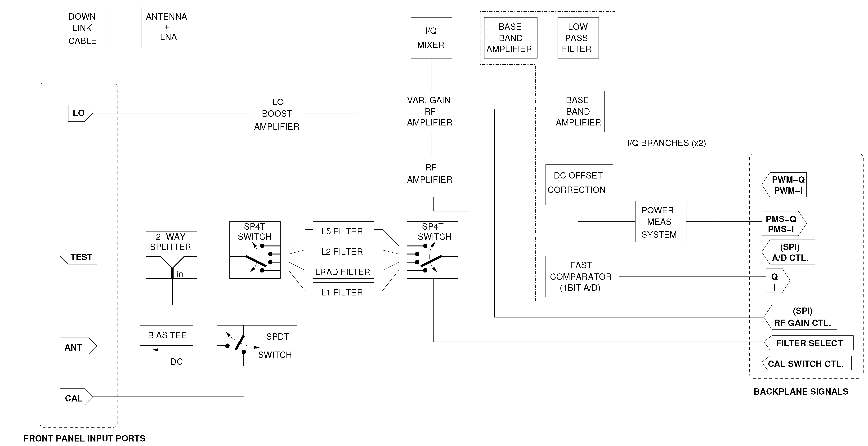
The custom designed RF receivers (see
Figure 2) are monitored and managed by the instrument controller. Each receiver has two input connectors: one for the antenna signal and one for the calibration signal. The receiver provides the power for the active antenna element pre-amp through a bias tee. A single-pole, double-through switch selects between the antenna and the calibration port. The signal passes through a two-way splitter, one output branch goes to the test connector of the receiver, and the other one is fed into a four-way filter bank to select one of the four frequency bands (L1 = 1575.42 MHz, L2 = 1227.60 MHz, L5 = 1176.45 MHz, LRAD = 1413 MHz). The filtered signal is amplified by two amplifier stages, one of which is digitally adjustable within a range of 31.5 dB. The signal is then down-converted to IF (≈19 MHz) using in-phase and quadrature branches, and these components are then low-pass filtered (35 MHz) and further amplified. A DC-offset compensation circuit sets the DC component of the signal (see
Section 2.2.1). The total power of the signal is measured by the Power Measurement System (PMS) (see
Section 2.2.2). Finally, a fast comparator quantizes the in-phase and quadrature components with one single bit each. Sampling at 80 MHz is effectively achieved at the input of the FPGA using D-type flip-flops.
2.2.1. DC Offset Compensation
The fast comparators used for digitizing the down-converted signals have an instrumental DC bias of only a few millivolts, but this DC offset becomes important for the latter post-processing when employing the PARIS interferometric technique. The resulting complex amplitude waveforms are displaced from the origin [
11], which effectively reduces the SNR (Signal to Noise Ratio) of the waveforms. When using the clean-replica processing this effect does not appear because the GNSS chipping codes are effectively DC free, and the DC bias is eliminated when computing the cross-correlation between the signal and the chipping code.
The function of the DC offset compensation circuit is to add a DC voltage to the signals with the opposite sign and the same amplitude as the instrumental DC offset. In a closed-loop approach, the instrument controller measures the DC component of the digital signals in real-time and for sequential periods of 1 s, and then generates a pulse-width modulated (PWM) signal for each in-phase and quadrature component, from which the DC offset compensation circuit extracts the DC value and subtracts it from the analogue signal.
2.2.2. Power Measurement System
Due to the one-bit per sample quantization, the amplitude information of the recorded signals is lost [
12]. In order to be able to recover this information, the root mean square (RMS) total power of the signals is measured by the circuit. It consists of an analogue multiplier that squares the signal, followed by a low-pass filter with a cut-off frequency of approximately 2 Hz. The resulting low-frequency voltage, which is proportional to the RMS power of the signal, is digitized using 16 bits and sampled at a 1 Hz rate.
2.3. Clock Synthesizer
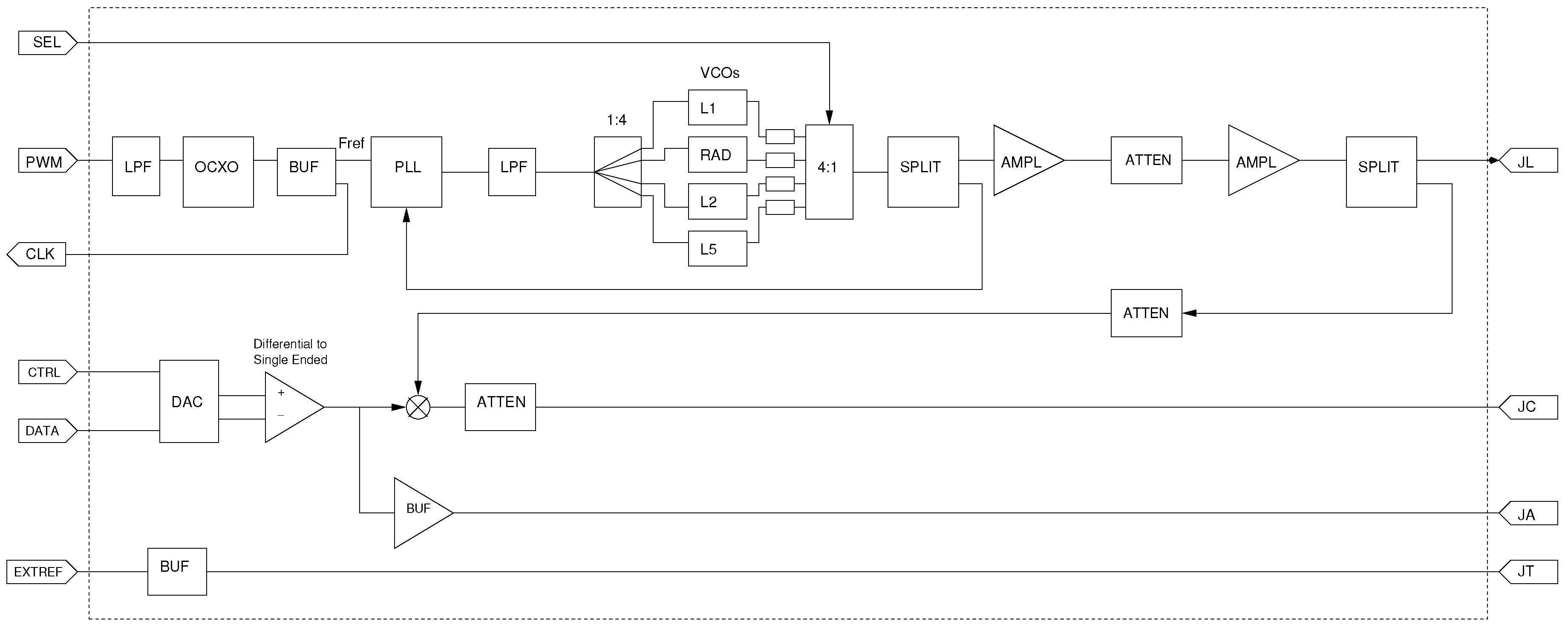
A block diagram of the in-house designed clock synthesizer is shown in
Figure 3. An oven controlled crystal oscillator (OCXO) generates the 100 MHz reference clock from which the local oscillator and the sampling frequency are derived. Its actual frequency can be slightly adjusted by the controller system, by using a PWM signal, which is low-pass filtered at the input of the OCXO. The reference clock is split into two: the first replica is delivered to the FPGA, which internally generates the 80 MHz sampling clock, and the second one is used to generate the local oscillator, through a phase-locked loop (PLL) and a bank of voltage controlled oscillators, one for each instrument band. The local oscillator is then amplified in several stages and delivered to the 16 receiver chains using an external 1:16 passive splitter. A digital calibration signal (pseudorandom noise with Gaussian statistics) provided by the controller is converted to the analogue domain and shifted to RF by using a passive mixer and a replica of the local oscillator. An external reference clock at 10 MHz, coherent with the 100 MHz clock, is also generated at the controller system and buffered through the clock synthesizer board. The function of this clock is to provide a coherent reference to the external electronics, so that the recorder can be used at higher frequency bands using external Low Noise Blocks (LNB). This will enable the use of SPIR with sources of opportunity at different frequency bands in the future.
2.4. Time-Tagging
Data is recorded with precise time-tagging information obtained from a GPS receiver and a navigation antenna (see
Figure 1). This GPS receiver provides 1PPS pulses synchronized to UTC time, as well as time and position observables in NMEA (National Marine Electronics Association) format.
2.5. Control and Recording System
At the beginning of the project, no commercial high-speed recording solution that would fit our needs (320 MB/s sustained recording with time-tagging and flexible front-end control) was available. Thus, we implemented our own high-speed control and recording system, which turned out to be the major technological bottleneck of the project.
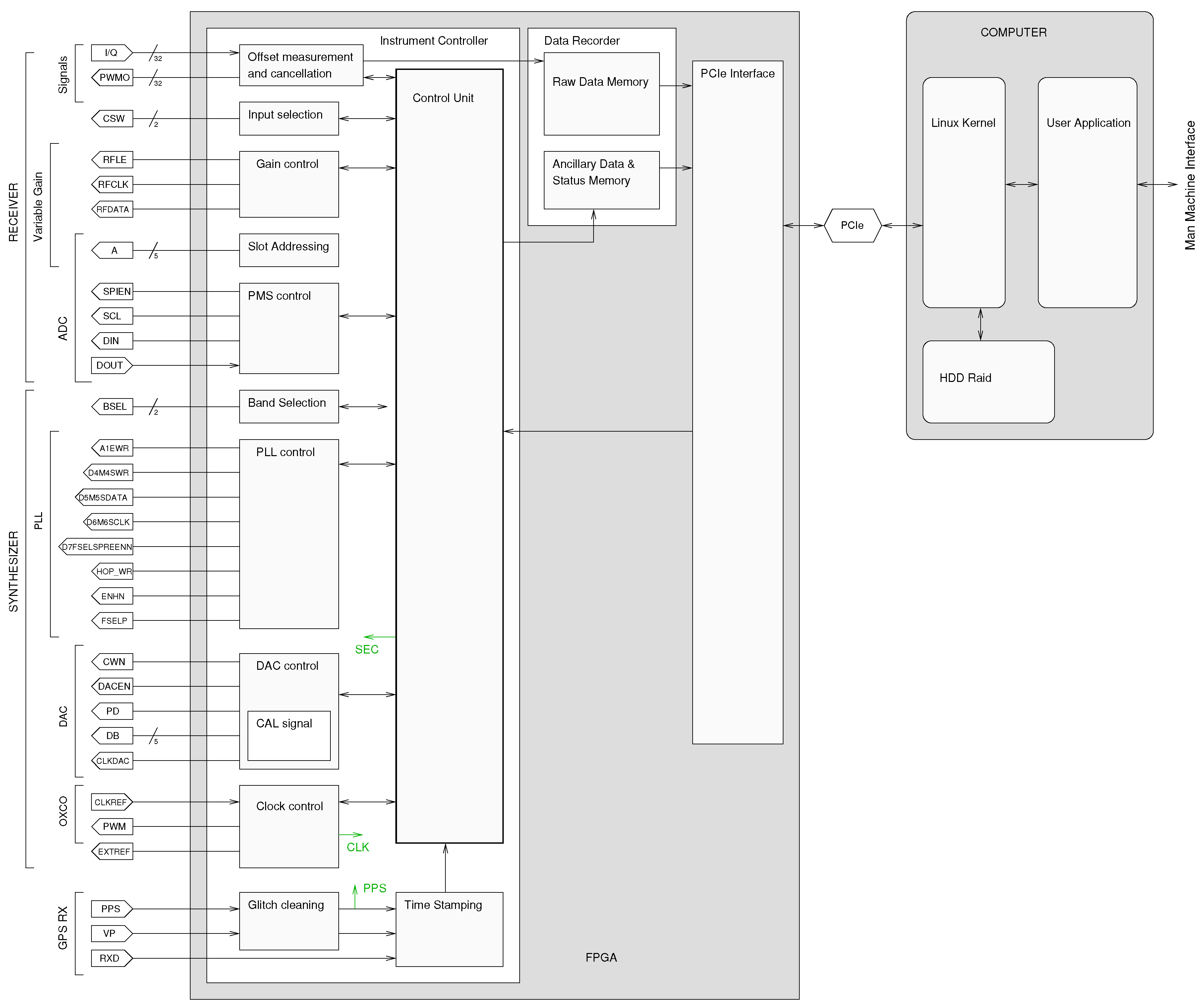
The control and recording system consists of an industrial computer running Linux with a DE4-Terasic development board inserted into one of the PCIe slots. The DE4 board is populated with a Stratix IV FPGA and its function is to interface with the SPIR front-end to control and program the different subsystems, in addition to gathering the 16 digital data-streams to be recorded on the computer. Although these two functions are clearly different (control and data recording), they have been implemented in one single FPGA and computer system. The reason for this implementation is that both actions need to be well synchronized, and this can be better achieved by implementing them in the same subsystem.
Figure 4 shows a block diagram for the control and recording system. The FPGA contains three subsystems: the instrument controller, the data recorder, and the PCIe interface of the computer. The implementation has been achieved using VHDL.
2.5.1. Instrument Controller
The instrument controller is the fundamental subsystem that makes it possible to achieve a sustained data recording rate of 320 MB/s (2.56 Gb/s) with exact time-tagging information for each recorded sample. Thus, we will now provide a detailed description on how this performance is achieved.
The core of the instrument controller is the main control unit responsible for the synchronization of all other blocks. The temporal coordination of the different activities is completed by two nested loops that are continuously repeated: a major cycle with a one-minute duration consists of 60 minor cycles of one second each. The instrument has three operation modes: (i) automatic: During the first second of every UTC minute, the instrument performs calibration measurements, and during the remaining 59 s, it pursues antenna measurements; (ii) calibration: The instrument performs only calibration measurements; and (iii) antenna: The instrument only performs antenna measurements.
The one-second cycles start with the 1PPS mark delivered by the GPS receiver, and its objective is to perform a regular set of actions to program and monitor the status of all subsystems of the SPIR, in addition to collecting the raw data. The sequence of actions during the one-second cycle controlled by the Control Unit is (see
Figure 5):
Read and save the data to the ancillary data and status memory in the following order:
- (a)
Offset measurements, offset PWM programming values and DC compensation steering mode.
- (b)
Gain control status data.
- (c)
PMS measurements.
- (d)
Band selection status.
- (e)
PLL status data.
- (f)
DAC (Digital to Analogue Converter) control and calibration signal status.
- (g)
Reference clock frequency measurement data.
- (h)
NMEA navigation data message.
Read the programming values for the next second from the PCIe interface and configure the sub-blocks.
Wait for the next 1PPS mark.
Additionally, synchronously with the 1PPS marks, the sub-blocks accept the new programming values, and if they have changed, they reprogram the SPIR front-end at the start of each second. The Control Unit also provides information on the current second within the major 60 second loop. This is especially important for the automatic calibration mode, where at the first second of each minute, the input switch of the receivers selects the calibration port, and the synthesizer board activates the calibration signal that is delivered to all of the receivers. Otherwise, the instrument always operates either in antenna mode or in calibration mode.
The function of the sub-blocks is shown in
Table 1.
2.5.2. Recorder
The data recorder’s function is to write the 16 data streams to the raw data memory and send its content, as well as the content of the ancillary data and status memory, to the computer through the PCIe bus. The data recorder also works in 1 s cycles, whose start is determined by the 1PPS marks. When the recording is started, it waits until the next 1PPS pulse is active to transmit the data of a full second to the computer, and once completed, it sends the packet of ancillary data that has been prepared by the instrument controller during that second. After that, it waits until the next 1PPS pulse to start the transmission of the next second of data. From this approach, it is clear that the last fraction of data for every second is never recorded, as this short interval of time is needed for sending the ancillary data (time-tagging, instrument status, etc.). In addition, this approach guarantees to have the same amount of data for each second, independently of the actual sampling frequency, which is derived from the actual system reference frequency. When the recorder is in the STOP mode, it behaves exactly as it does in the RECORD mode, except that it skips the step which sends the raw data.
Raw-Data Transmission
The raw data is composed of the 16 in-phase and quadrature 1-bit sampled signals output by the eight up-looking and eight down-looking antennas/receivers. These signals provide a 32-bit stream of data, sampled at a rate of 80 MHz. Therefore, the data recorder deals with a sustained stream of 320 MB/s.
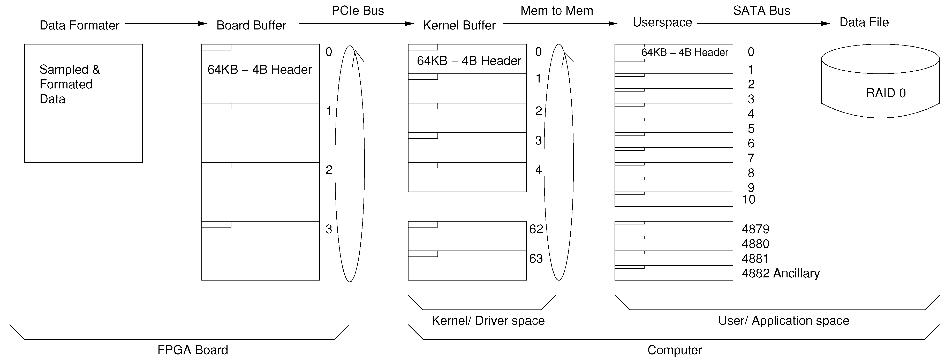
Ideally, one would transmit the complete amount of data in 1 s using a single transfer to the computer, but memory limitations within the FPGA and DMA (Direct Memory Access) micro-transfers through the PCIe bus force the continuous stream to split into smaller data units of 64 KiB. The first 4 bytes of these blocks are used as an identifier field (ID), and the remaining 64 KiB-4 bytes correspond to raw data. This ID is used to determine the beginning of a second and the block position within the file, and to check the integrity of the collected data.
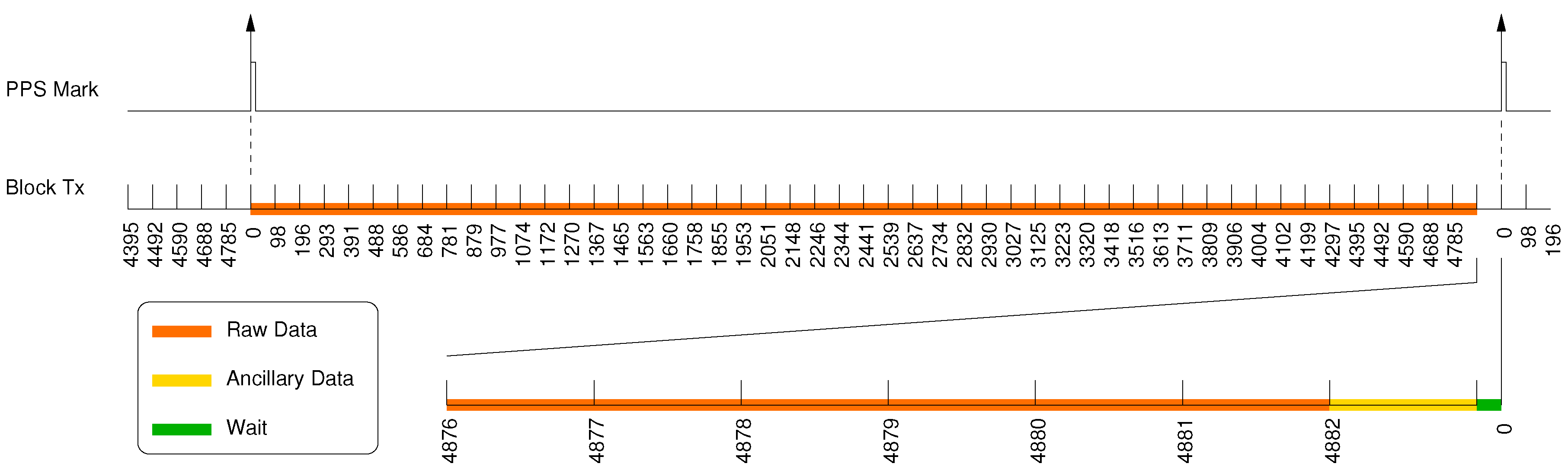
The 320 MB of data of each second are divided into blocks of 64 KiB-4 bytes = 65,532 bytes, which results in 4883.1105 blocks for every second. As only complete blocks can be sent through the PCIe bus, and the last block is used to transmit ancillary data instead of raw signal data, the total amount of raw data blocks transmitted is 4882. Thus, the actual amount of recorded raw data is 319,927,224 bytes, which corresponds to 99.98% of the available data. The raw data gap has a duration of 227 .
The transmission sequence of blocks from the data recorder module through the PCIe interface is shown in
Figure 6. In the recording mode, when a 1PPS pulse is received, the data recorder transmits 4882 blocks of 64 KiB-4 bytes of raw data through the PCIe bus, plus one block of ancillary data. Then, the data recorder waits until the next PPS pulse to transmit a new second of data.
The recorder generates a synchronization signal, which is active at the start of the transmission of the ancillary data. This synchronization signal is used by the Instrument Controller to reprogram the different sub-modules with the new programming values.
The use of 64 KiB blocks allows using circular buffers at the different stages of the data transmission from the FPGA towards the file in the PC hard disk. The different stages are shown in
Figure 7. The first stage collects and formats the data into blocks (64 KiB) with the ID according to the current instant. Each of these blocks is then transferred to the circular buffer of four blocks within the FPGA. The block is stored until the PCIe-DMA transfer is triggered, which is when the block is sent to the kernel memory space allocated by the Linux driver. Similar to the FPGA circular buffer, the kernel memory is structured in a circular buffer of 64 blocks (4 MiB). At this point, the user application is in charge of emptying the driver circular buffer and arranging the blocks (using their ID) to build the one-second files in RAM. Once a complete second has been received, it is written to the computer’s hard disc for later post-processing. A RAID 0 array of disks is used to achieve a high-speed writing with medium-speed disks, as actual writing to the individual disks is done in parallel in RAID 0.
Using pointers and circular memory buffers enables one to automatically transfer the new data to the next stage by polling. This approach was selected to ensure that the later stages (right in
Figure 7) retrieve the data as soon as it is generated at the previous stage, avoiding an overrun of the buffers of previous stages.
Clock-Ticks Counter
The data recorder has a counter that is set to zero on start-up, to count the total number of clock ticks that have elapsed since the recorder was started. The clock tick corresponding to the first tick within each second is stored in the ancillary data block. In this way, it is possible to link the time (ticks) of consecutive seconds, despite the fact that the last part of the second is not recorded. This mechanism provides the means necessary to maintain data continuity without compromising the synchronism with the 1PPS pulses.
2.6. Offline Signal Processor
This section describes the two main post-processing steps applied to the SPIR raw data set to obtain waveforms, which are the main observables in GNSS-R: a beamformer and a correlator. It is worth mentioning two aspects at this point:
We only consider here the case of an up-looking antenna tracking a given GNSS satellite and a down-looking antenna tracking the corresponding specular point of reflection over the Earth’s surface. However, other options could be also envisaged with SPIR, such as the observation of areas far from the specular one with the down-looking antenna.
The description on how to obtain waveforms from the beamformed signals is based on the interferometric approach or iGNSS-R (i.e., direct cross-correlation between direct and reflected signals) [
2,
3], but other processing approaches, such as the GNSS-R clean-replica e.g., [
6], partial interferometry [
13] or semi-codeless [
14], can be also attempted with the SPIR raw dataset.
2.6.1. Beamformer
The purpose of the beamformer is to maximize the antenna beam gain towards the desired direction. It is achieved by combining the signals of the different antenna elements with a proper phase shift. Thus, the first step is to obtain the phases to be applied.
The basic idea behind this concept is to coherently add the different contributions from the same signal source sensed at the different antenna elements. Given that their positions are separated by distances of an order of magnitude of the wavelength, the phase-delay for each antenna, which depends on the direction of arrival, must be compensated for. These compensations, called beamformer phases hereafter, can be seen as phase rotations applied to the signals detected at each antenna element in order to align them to a reference (differential measurement). Two different methodologies for the computation of these phases are described next, while the approach that is finally adopted is explained afterwards.
Theoretical Method
By knowing the precise positions of the transmitter and the receiving antenna elements, we can simply compute the beamformer phases as the delay path difference between the transmitter to the array element and the transmitter to the reference element in the array as multiples of wavelength cycles.
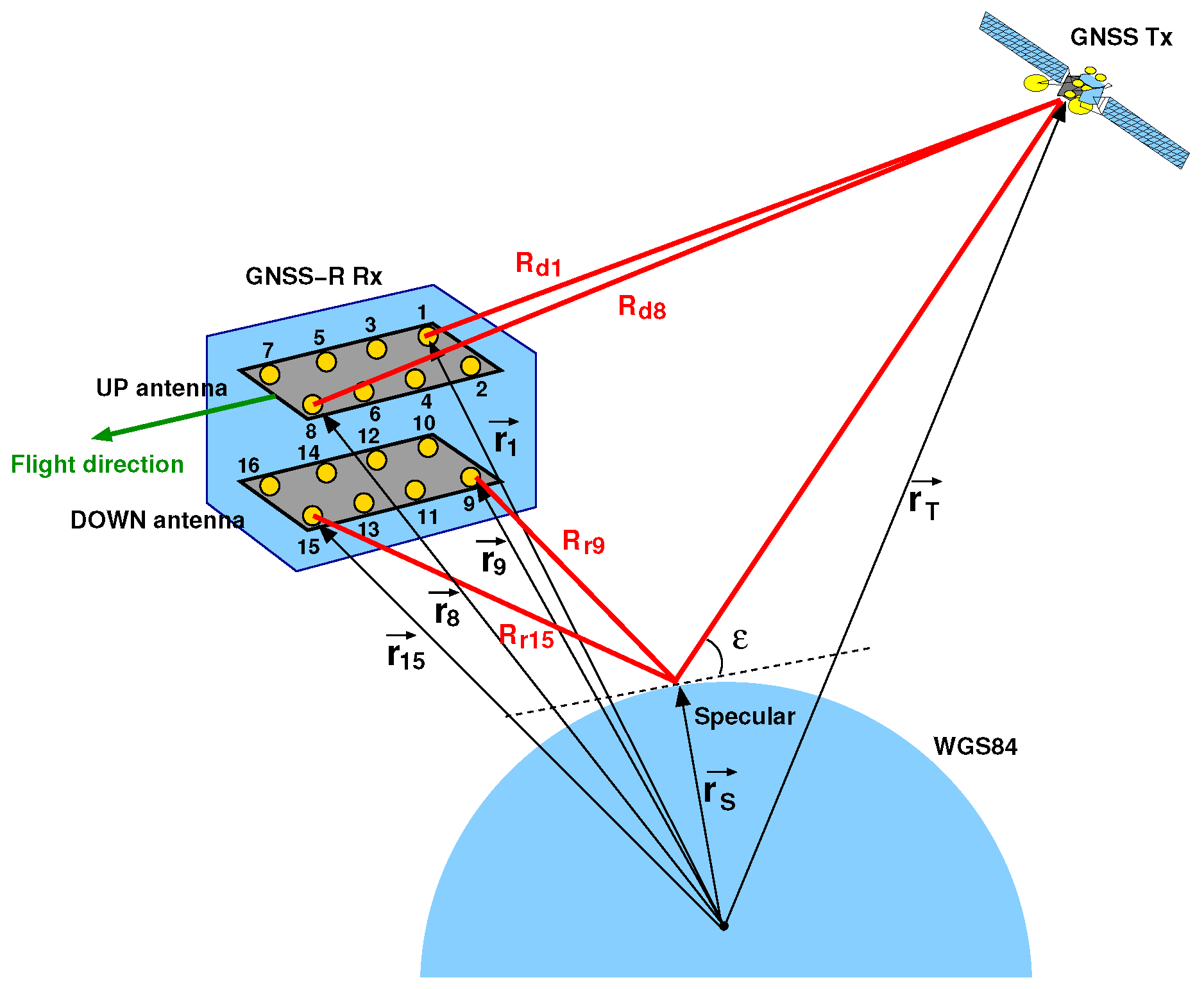
Figure 8 shows a scheme of the delay path distances involved in this method, particularly applied for a typical SPIR experimental scenario. While the up-looking array points towards a given GNSS satellite, the down-looking array points towards its corresponding reflection at the surface of the sea. The beamformer phases for the up-looking array are expressed as relative phases with respect to the first antenna element in the array and are given by:
with
i being the element number (from one to eight),
representing the delay path distance of the direct signal for element
i,
being the vector of the position of element
i and
representing the vector of the position of the transmitter (GNSS satellite), both in an ECEF (Earth-Centered, Earth-Fixed) coordinate system.
Similarly, the beamformer phases for the down-looking array are expressed relative to antenna element number nine and are given by:
with
i being the element number (from nine to 16),
representing the delay path distance of the reflected signal for element
i,
being the vector of the position of element
i and
representing the vector of the position of the specular point over a geoid model (ellipsoid WGS84), both in an ECEF coordinate system. We can assume that the position of the specular point does not vary for the different array elements given the high altitude of the GNSS satellite compared to the array baseline and the receiver’s height.
This method compensates for the geometrical phase differences, but does not correct instrumental antenna phase differences.
GNSS-Tracking Method
The development of this method was motivated as a solution to beamformer pointing without a knowledge of the precise position and orientation of the arrays. The method relies on the properties of the GNSS signals, and the idea is to apply the clean-replica approach at each antenna element and to compute the phases that align in the complex plane all obtained waveforms to the reference. This is done for each array individually. Therefore, for each antenna array, the process consists of:
Selection of a visible PRN (Pseudo-Random Noise) transmitter to point towards.
Obtain the Doppler frequency of the selected PRN by computing the cross-correlation using the FFT of the reference antenna signal and the clean-replica code modulated with a carrier tone over a given frequency range. The Doppler frequency of the signal corresponds to the one that maximizes the amplitude of the correlation function.
FFT-based cross-correlation of the data from each antenna element with the clean-replica code modulated with the Doppler obtained to generate a complex waveform for each case.
Computation of the beamformer phases as the differences between the phases of the complex waveform’s peaks for each antenna element against the same term at the reference element.
Notice that this method also compensates for the remaining instrumental offsets of the system. On the other hand, this technique is computationally costly, and it is affected by the signal’s noise and other factors such as multipath.
Selected Approach
After taking into account the trade-offs of each method, the solution adopted combines both. During the first stage, the GNSS-tracking method is employed to retrieve the beamformer phases during certain tracks with a proper visibility and high SNR. Then, by assuming that the instrumental phases are not affected by the geometry (they shall be the same for different PRNs), we can obtain them as the average difference between the beamformer phases provided by the theoretical method and those phases obtained with the GNSS-tracking method. Once the instrumental offsets have been estimated, the theoretical method, which is computationally faster and not affected by multipath and noise, is employed to obtain the corrected beamformer phases to properly combine the signal contributions of the different channels in the antenna array. The beamformer phases are updated every second for both up- and down-looking antenna arrays.
2.6.2. Interferometric Correlator
For every millisecond
, the complex raw samples from SPIR’s front ends are combined to obtain the up and down-looking beamformed signals as:
where
i denotes the antenna element number,
is its corresponding complex signal component for the time series of
ms, and
is its beamformer phase at millisecond
.
The next step consists of cross-correlating both signals at the output of the beamformers in the frequency domain by using FFTs. We transform the time-domain signal to the frequency domain and compute the complex conjugate product of their spectra. Before returning the result to the time domain, we apply a comb-like filter
to remove interfering tones. The bandwidth is set according to the nominal values for each type of signal (GPS/Galileo at L1/L5). Therefore, for every millisecond
and set of
, we obtain the complex waveform:
where
and
are the discrete Fourier transforms (
) of
and
respectively, and
is the filter applied.
Finally, coherent (complex sum) and non-coherent (power averaging) integrations are performed in order to reduce thermal noise and speckle. The coherent and non-coherent integration intervals are programmable. Before each integration process, the waveform series are aligned with respect to the first sample (retracking), based on a precise altimetric delay model. This is done in order to compensate for the movement of the aircraft in the vertical direction during the integration period. Not doing so would result in smeared correlation waveforms along the horizontal delay axis. In order to avoid the use of interpolation methods between samples, this step is also done in the frequency domain. We use the Fourier transform property, by which a delay in the temporal domain is equivalent to a phasor multiplication in the frequency domain [
15].
2.7. Implemented Instrument
The implemented instrument is shown in
Figure 9 and has been used in several airborne campaigns (not described in this paper) in support of space-borne GNSS-R research, in particular the GEROS-ISS mission [
4]. A compact version of SPIR, called SPIR-UAV, has also been implemented on-board an unmanned aerial vehicle (UAV) to gather GNSS reflections over sea ice in the Arctic. To reduce the mass and power consumption, the antenna arrays of SPIR-UAV consist of six elements each, instead of the eight elements of SPIR, and the control and recording computer has been integrated close to the RF receivers. The SPIR-UAV is also shown in
Figure 9.
3. Instrument Validation
In this section we present the performance results of the SPIR instrument and its subsystems including the software processor.
3.1. Reference Clock Steering
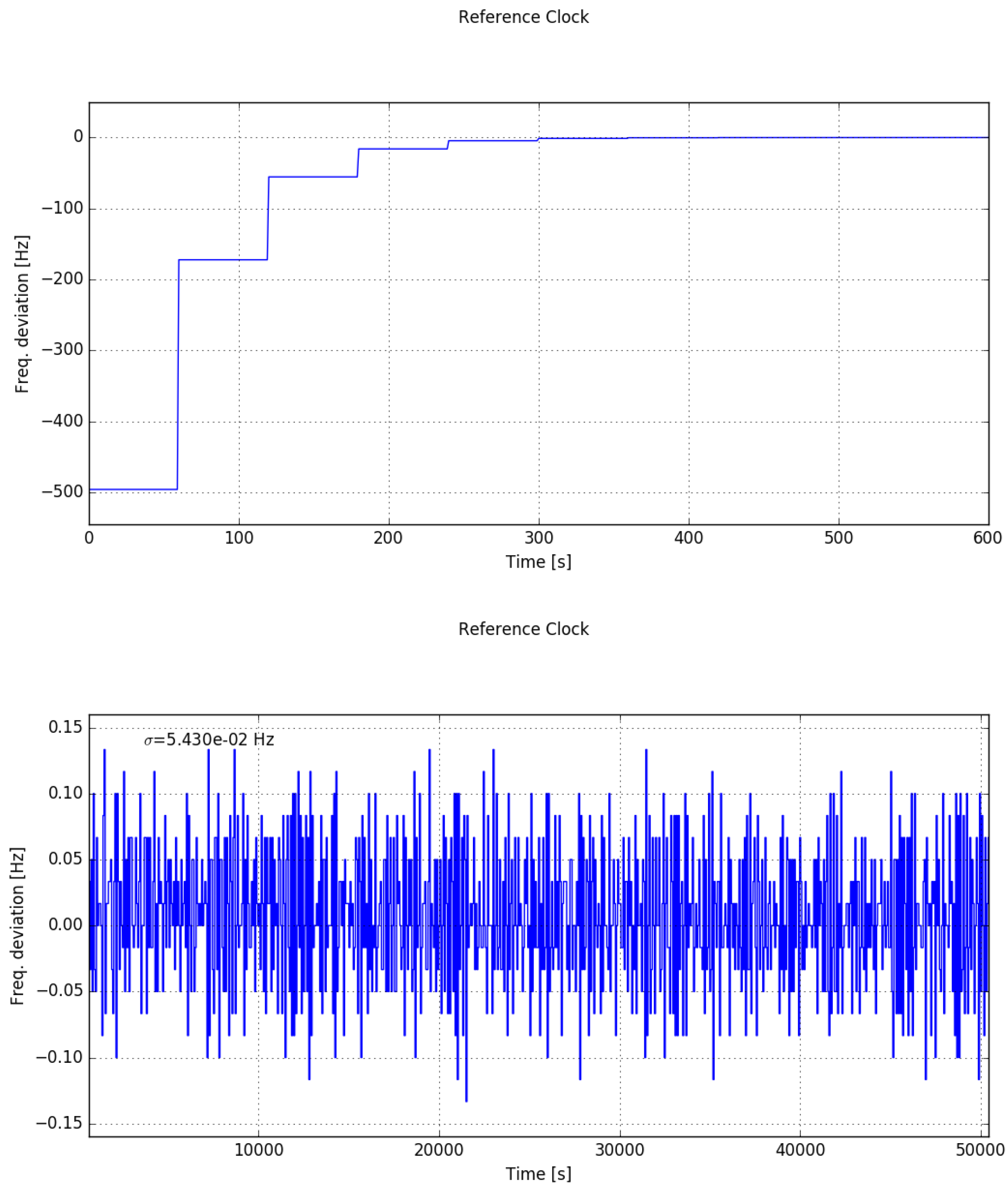
The clock steering loop takes less than 10 min to adjust the system reference frequency at its nominal value.
Figure 10 shows the reference clock frequency evolution. The upper plot zooms into the first 10 min where the clock frequency converges towards its nominal value, while the lower plot shows the steady state regime. The standard deviation of the stabilized reference clock frequency is below 0.06 Hz for a period of 14 h.
3.2. DC Offset Compensation
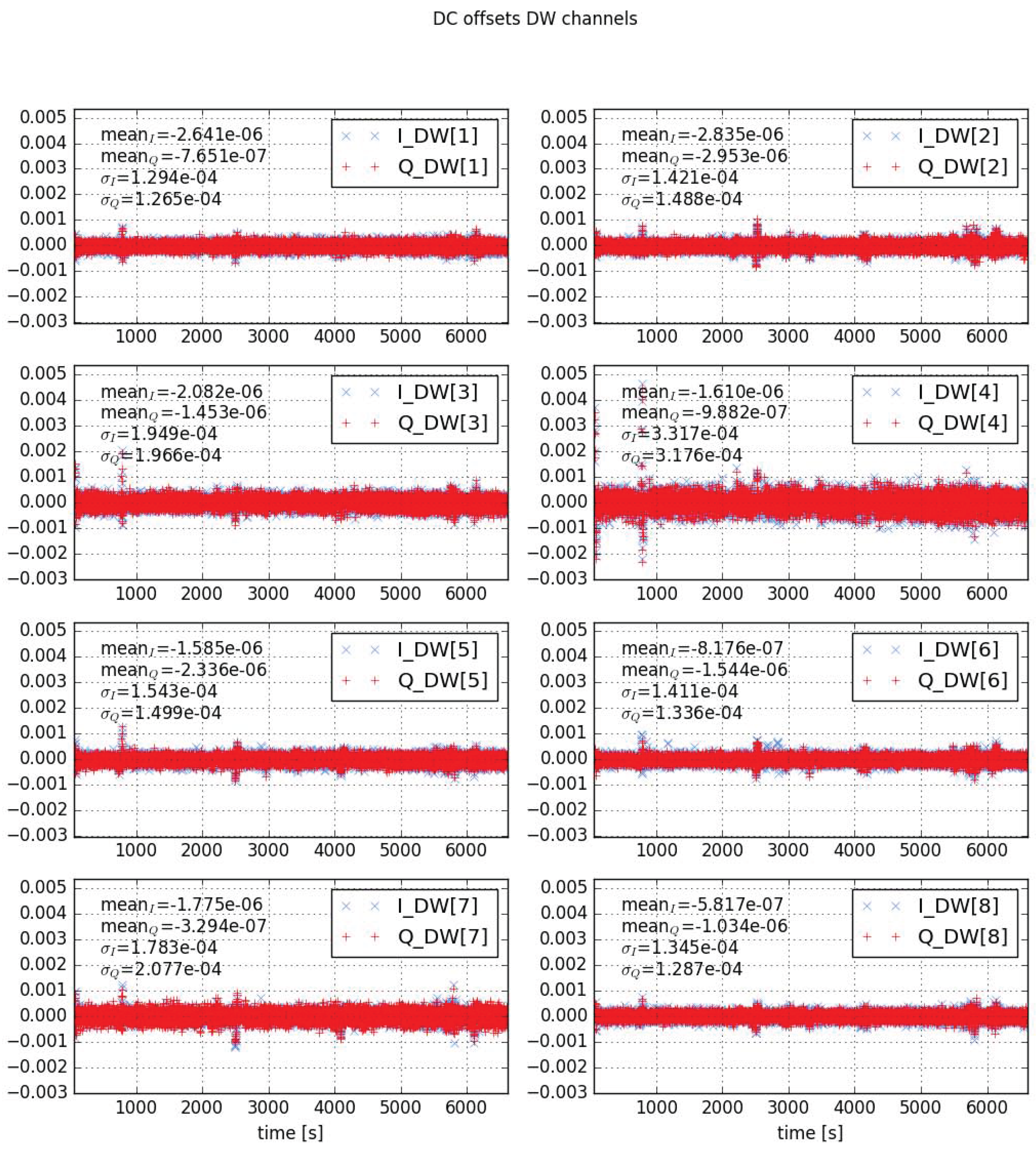
The DC offset compensation circuit is capable of driving the DC offsets of the input signals to zero in less than 20 s.
Figure 11 shows the DC offsets in a steady state regime for the eight up-looking channels during a scientific flight over the Baltic Sea in December 2015. The theoretical standard deviation of the DC offset measurements when the actual offset is zero can be computed using basic statistics and is given by
, where
N is the number of independent samples used to estimate the offset. The DC offsets are estimated every second, so using
samples and taking into account that the noise equivalent bandwidth of the receivers is 34 MHz, the number of independent samples is reduced to
which results in an expected variance of
. The measured standard deviation of the offsets is in the range between
and
, and this shows that the offset compensation circuit is working almost the same as in the ideal case.
From
Figure 11 it can also be appreciated that some spikes, which are coincident in all channels, happen at particular instants. We have verified that these happened when the airplane was turning, which resulted in off-nadir antenna pointing. Whether the DC offset compensation spikes are attributed to a change in the input signal power due to off-nadir antenna pointing or due to the external interferences acquired during these turns remains unclear. Spectral analysis of the collected signals during the intervals is precluded by the fact that raw-data recording was switched off when the airplane was turning.
3.3. Power Measurement System
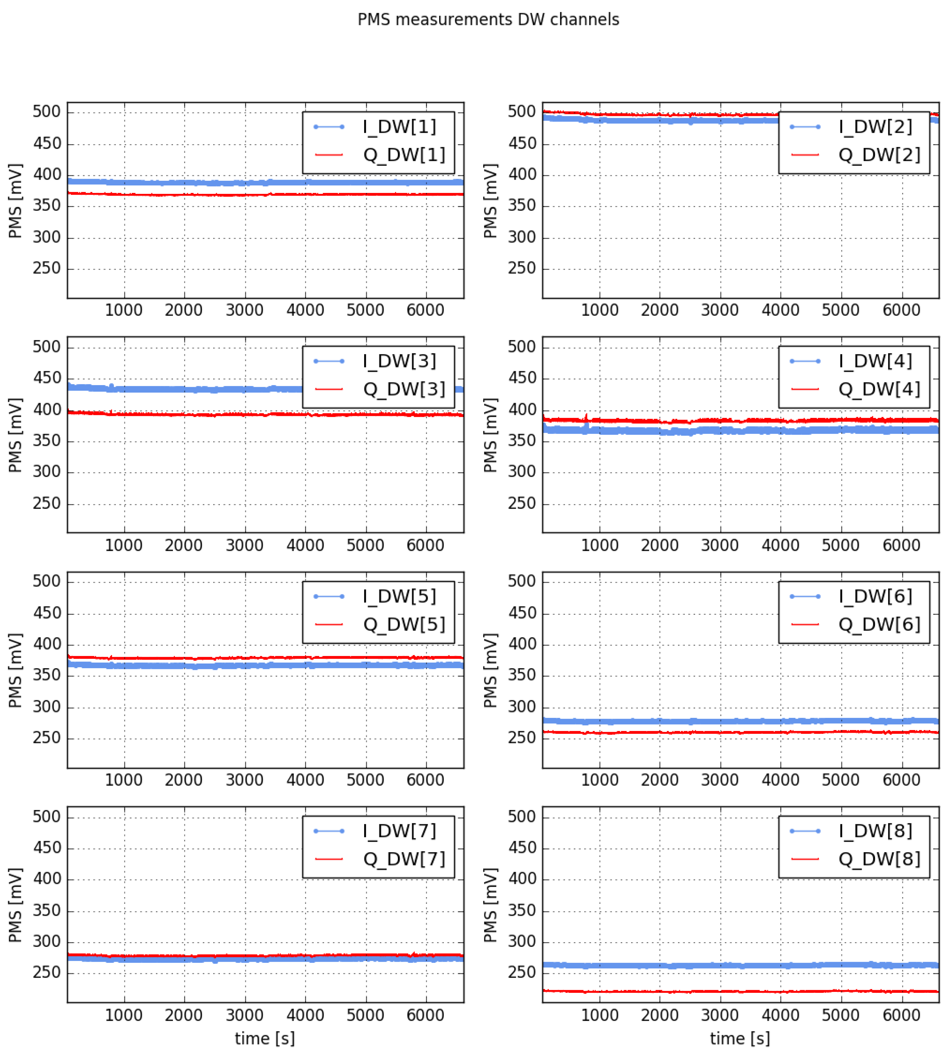
Figure 12 shows the PMS measurements for the flight of December 2015 for all down-looking channels. These are stable, as expected for a sea surface target, although they show small variations that are coincident with the peaks measured in the DC offset correction system. The mean value for all of the PMS measurements is different. This is due to the tolerances of the electronic components building the PMS circuit, and it is not critical, as the differences can be characterized through the calibration procedures of the instrument.
4. Data Set Examples
In this section we present sample data acquired and processed with the SPIR instrument and software processor in an airborne experiment over the Baltic Sea at a 3000 m altitude in December 2015.
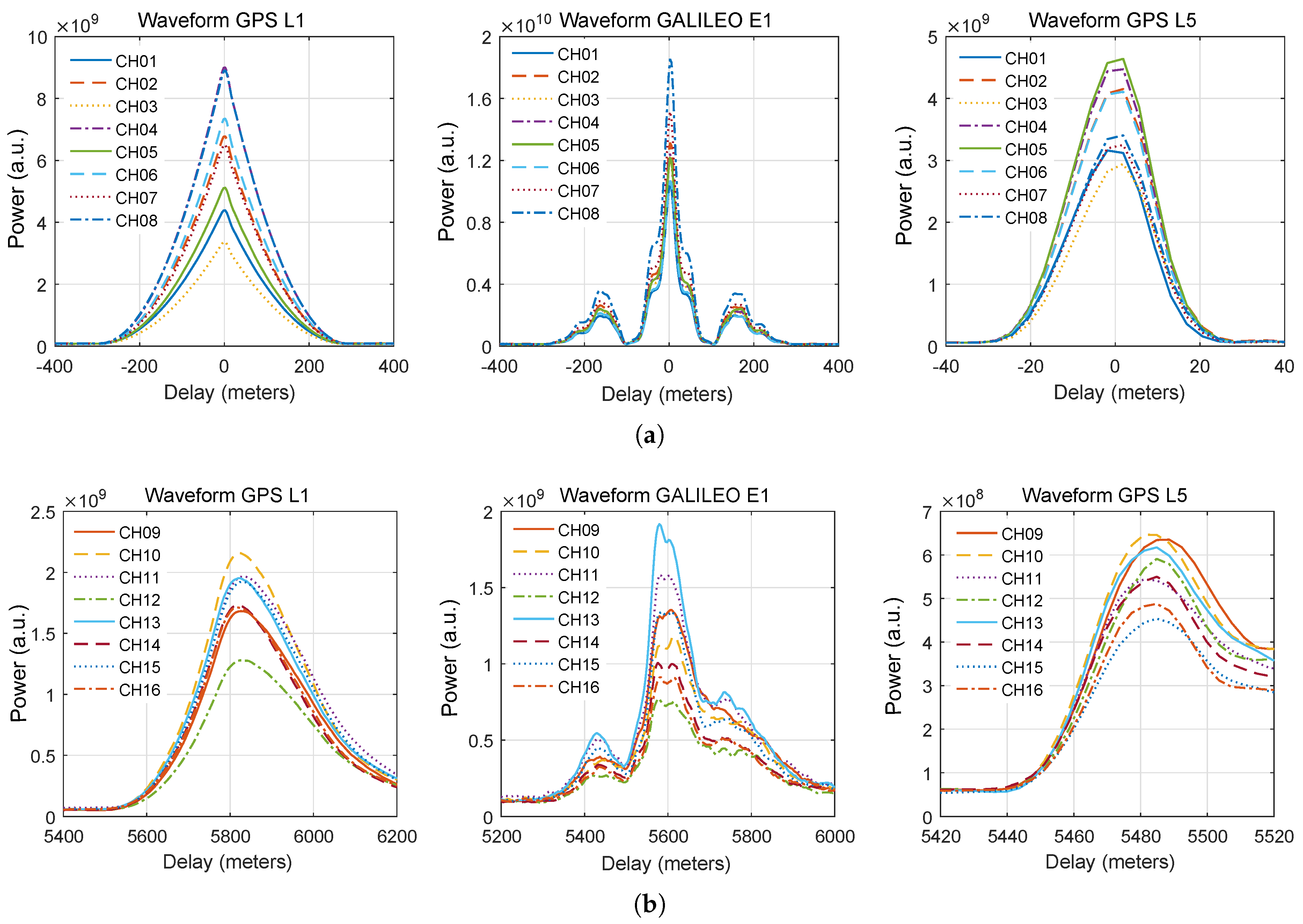
Figure 13 shows example power waveforms obtained when using clean-replica processing for each antenna element individually, employing a coherent integration time of 1 ms and a non-coherent integration of 1 s. The upper row corresponds to the eight up-looking antennas and the lower row for the down-looking ones, and from left to right GPS L1, Galileo E1 and GPS L5, using the corresponding publicly available chipping codes. The shape of the obtained waveforms is consistent with theory, and only amplitude variations, which are caused by gain and noise figure variability among receiver channels, can be observed. For GPS L1, we can clearly appreciate the shape of the C/A waveform. For Galileo E1, the waveform has a more complex shape due to the sub-carrier modulation. For GPS L5, the waveform is much narrower than for the previous two cases (note the different horizontal axis in the plot), as the chipping rate is 10.23 MHz instead of 1.023 MHz. The SNR values for the different waveforms are shown in the caption of the figure.
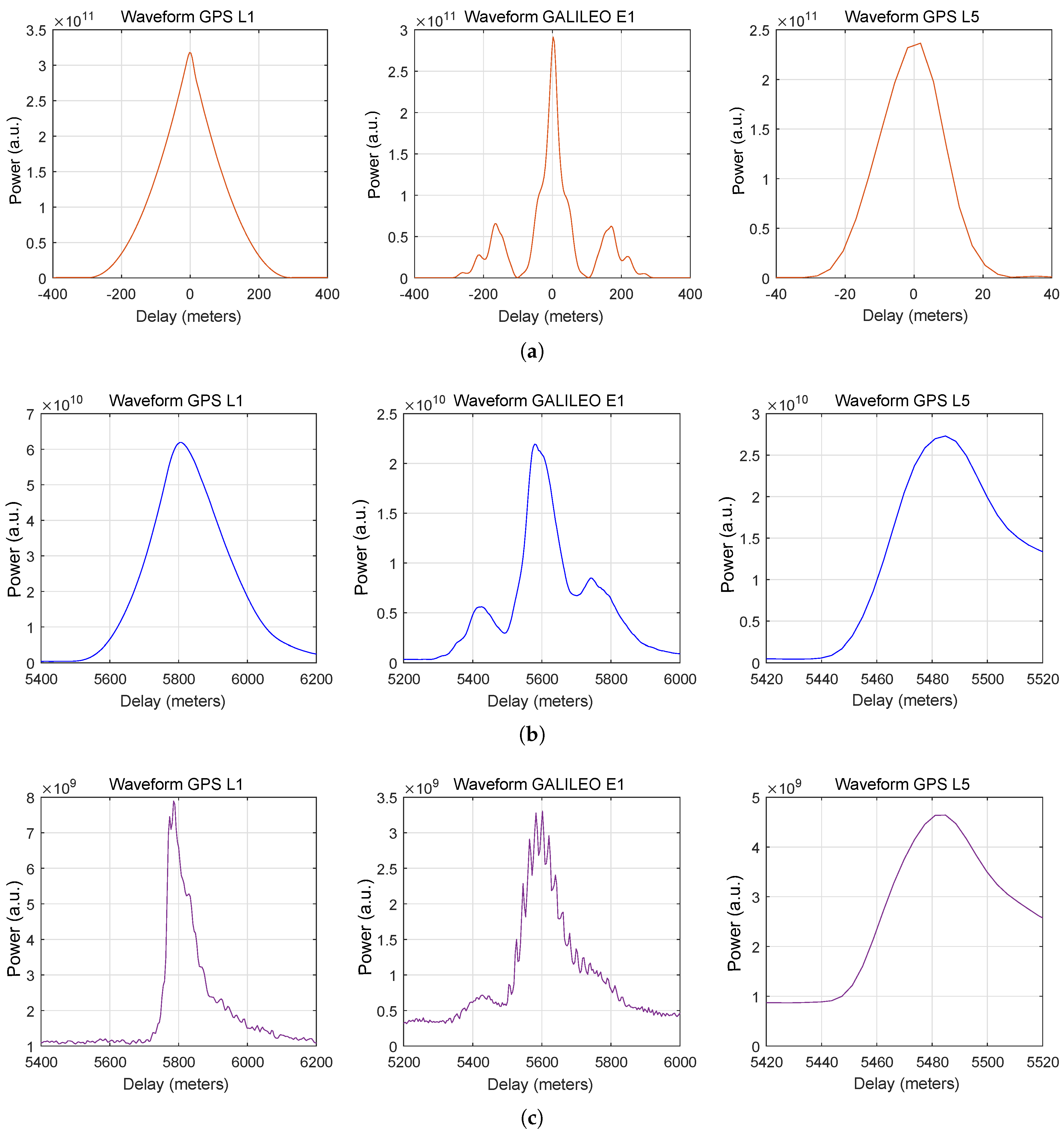
Figure 14 shows the obtained waveforms after beamforming for the up and down-looking antenna arrays. The first row corresponds to the clean-replica waveforms obtained by the up-looking antenna array, while the second row corresponds to the clean-replica waveforms obtained using the down-looking antenna array. The third row shows the waveforms obtained using the interferometric technique. Again, from left to right, the waveforms correspond to GPS L1, Galileo E1, and GPS L5 acquisitions. The coherent and non-coherent integration times were 1 ms and 1 s, respectively. The obtained waveforms are coincident with the expected ones also in this case. It can be clearly observed that the resulting waveforms for GPS L1 are much narrower than for the clean-replica processing, as the full bandwidth of the transmitted signals is used, including the P and M chipping codes. For Galileo E1, we can also observe the
ripples on top of the waveforms, whose origin is the Galileo E1-A code, which has a sub-carrier modulation.
The presented results show that the instrument is capable of adequately acquiring and processing the signals with proper beamforming, and obtaining waveform observables using the clean-replica and interferometric processing methods indistinctly.
5. Conclusions
We have designed and implemented a GNSS-R instrument called SPIR with the objective of providing a way to demonstrate the synoptic capabilities of the PARIS interferometric technique. Therefore, we have designed and built an instrument capable of acquiring GNSS signals from two antenna arrays of eight elements each and recording them onto an array of hard disks. The signals of each antenna element are individually down-converted coherently to IF (in-phase and quadrature) with an RF bandwidth of about 35 MHz, sampled at an 80 MHz rate, and quantized using one bit per sample. Data is precisely time-tagged and recorded at a sustained rate of 320 MBytes/s (2.56 Gbits/s) during a period of up to three hours. The instrument can operate at L1, L2, and L5 GNSS bands, and its operation can be easily expanded to higher frequency bands by the coherent heterodyne down-conversion to L-band. Signal processing and data-analysis is done off-line, using a specially designed signal processor that performs digital beamforming and signal correlation. This signal processor currently implements the clean-replica and interferometric GNSS-R techniques, which allows for an intercomparison of both techniques using exactly the same data.
We have demonstrated the performance of the instrument by presenting a variety of ancillary and monitoring data collected by the instrument itself in laboratory and airborne tests. Furthermore, we have also presented the clean replica and interferometric waveforms obtained in an airborne campaign over the Baltic Sea and processed using our signal processor.
The SPIR instrument has provided significant results in support of GNSS-R remote sensing, and in particular, the development of future space-borne GNSS-R missions such as GEROS-ISS by validating waveform models and altimetry retrieval techniques.
Acknowledgments
This work has been carried out with the financial support of the following research projects and contracts: Spanish research projects: AYA2011-29183-C02-02 (Ministerio de Economía, Industria y Competitividad) and ESP2015-70014-C2-2-R (MINECO/FEDER) , ESA Contract: RFQ/3-12747/09/NL/JD-CCN4, and the European FP7 project E-GEM (UE 607126). We would like to thank Aalto University’s Skyvan team for their contribution to the success of the airborne campaigns and to Ramon Padullés for his help in the campaigns.
Author Contributions
The instrument was designed and built by Serni Ribó, Juan Carlos Arco-Fernández and Oleguer Nogués-Correig. The signal processor and data-analysis studies were done by Fran Fabra, Weiqiang Li, Antonio Rius and Estel Cardellach. The experimental campaigns were planned and carried out by Serni Ribó, Fran Fabra and Manuel Martín-Neira.
Conflicts of Interest
The authors declare no conflict of interest.
References
- Hall, C.D.; Cordey, R.A. Multistatic Scatterometry. In Proceedings of the International Geoscience and Remote Sensing Symposium, IGARSS ’88. Remote Sensing: Moving Toward the 21st Century, Edinburgh, UK, 12–16 September 1988. [Google Scholar]
- Martín-Neira, M. A Passive Reflectometry and Interferometry System (PARIS)—Application to ocean altimetry. ESA J. 1993, 17, 331–355. [Google Scholar]
- Martín-Neira, M.; D’Addio, S.; Buck, C.; Floury, N.; Prieto-Cerdeira, R. The PARIS Ocean Altimeter In-Orbit Demonstrator. IEEE Trans. Geosci. Remote Sens. 2011, 49, 2209–2237. [Google Scholar] [CrossRef]
- Wickert, J.; Cardellach, E.; Martín-Neira, M.; Bandeiras, J.; Bertino, L.; Andersen, O.B.; Camps, A.; Catarino, N.; Chapron, B.; Fabra, F.; et al. GEROS-ISS: GNSS REflectometry, Radio Occultation, and Scatterometry Onboard the International Space Station. IEEE J. Sel. Top. Appl. Earth Obs. Remote Sens. 2016, 9, 4552–4581. [Google Scholar] [CrossRef]
- Rius, A.; Cardellach, E.; Martín-Neira, M. Altimetric Analysis of the Sea-Surface GPS-Reflected Signals. IEEE Trans. Geosci. Remote Sens. 2010, 48, 2119–2127. [Google Scholar] [CrossRef]
- Nogués-Correig, O.; Cardellach Galí, E.; Sanz Campderròs, J.; Rius, A. A GPS-Reflections Receiver That Computes Doppler/Delay Maps in Real Time. IEEE Trans. Geosci. Remote Sens. 2007, 45, 156–174. [Google Scholar] [CrossRef]
- Rius, A.; Fabra, F.; Ribó, S.; Arco, J.C.; Oliveras, S.; Cardellach, E.; Camps, A.; Nogués-Correig, O.; Kainulainen, J.; Rohue, E.; et al. PARIS Interferometric Technique proof of concept: Sea surface altimetry measurements. In Proceedings of the 2012 IEEE International Geoscience and Remote Sensing Symposium, Munich, Germany, 22–27 July 2012; pp. 7067–7070. [Google Scholar]
- Cardellach, E.; Rius, A.; Martín-Neira, M.; Fabra, F.; Nogues-Correig, O.; Ribó, S.; Kainulainen, J.; Camps, A.; D’Addio, S. Consolidating the Precision of Interferometric GNSS-R Ocean Altimetry Using Airborne Experimental Data. IEEE Trans. Geosci. Remote Sens. 2014, 52, 4992–5004. [Google Scholar] [CrossRef]
- Meehan, T.K.; Esterhuizen, S.; Franklin, G.W.; Lowe, S.; Munson, T.N.; Robison, D.; Spitzmesser, D.J.; Tien, J.Y.; Young, L.E. TOGA, a prototype for an optimal orbiting GNSS-R instrument. In Proceedings of the 2007 IEEE International Geoscience and Remote Sensing Symposium, Barcelona, Spain, 23–27 July 2007; pp. 5109–5112. [Google Scholar]
- Esterhuizen, S.; Meehan, T.K.; Robinson, D. TOGA—A GNSS Reflections Instrument for Remote Sensing Using Beamforming. In Proceedings of the 2009 IEEE Aerospace Conference, Big Sky, MT, USA, 7–14 March 2009. [Google Scholar]
- Ribó, S.; Arco, J.C.; Oliveras, S.; Cardellach, E.; Rius, A.; Buck, C. Experimental Results of an X-Band PARIS Receiver Using Digital Satellite TV Opportunity Signals Scattered on the Sea Surface. IEEE Trans. Geosci. Remote Sens. 2014, 52, 5704–5711. [Google Scholar] [CrossRef]
- Thompson, A.; Moran, J.; Swenson, G.W., Jr. Interferometry and Synthesis in Radio Astronomy, 2nd ed.; WILEY-VHC: Weinheim, Germany, 2004. [Google Scholar]
- Li, W.; Yang, D.; D’Addio, S.; Martín-Neira, M. Partial Interferometric Processing of Reflected GNSS Signals for Ocean Altimetry. IEEE Geosci. Remote Sens. Lett. 2014, 11, 1509–1513. [Google Scholar]
- Lowe, S.T.; Meehan, T.; Young, L. Direct Signal Enhanced Semicodeless Processing of GNSS Surface-Reflected Signals. IEEE J. Sel. Top. Appl. Earth Obs. Remote Sens. 2014, 7, 1469–1472. [Google Scholar] [CrossRef]
- Oppenheim, A.V.; Willsky, A.S.; Young, I.T. Signals and Systems; Prentice Hall International: Upper Saddle River, NJ, USA, 1983. [Google Scholar]
Figure 1.
Block diagram of the Software PARIS Interferometric Receiver (SPIR) hardware.
Figure 1.
Block diagram of the Software PARIS Interferometric Receiver (SPIR) hardware.
Figure 2.
Block diagram of the RF receivers of SPIR.
Figure 2.
Block diagram of the RF receivers of SPIR.
Figure 3.
Block diagram of SPIR’s clock synthesizer.
Figure 3.
Block diagram of SPIR’s clock synthesizer.
Figure 4.
Block diagram of the control and recording system of SPIR.
Figure 4.
Block diagram of the control and recording system of SPIR.
Figure 5.
Timing diagram for the instrument controller within the one-second cycle. Data recording and instrument control are done simultaneously and are started synchronously with each 1PPS mark. Raw data is recorded during from the beginning of each second, while ancillary data is saved at the end of each second (indicated with an “A” in the figure). Instrument control is carried out in a sequential way by different control blocks.
Figure 6.
Data Recorder GPS one-second cycle.
Figure 6.
Data Recorder GPS one-second cycle.
Figure 7.
Data Recorder data flux between stages.
Figure 7.
Data Recorder data flux between stages.
Figure 8.
Scheme of the beamformer theoretical method. This example shows the different components involved in the computation of the beamformer phases for elements eight and 15 (where one and nine are the reference ones) in the up- and down-looking arrays, respectively. The distribution of the antenna elements is displayed as in the real experiment.
Figure 9.
Left: RF front-end of the SPIR Instrument. The control and recording system is implemented in a standard industrial PC. Right: SPIR-UAV instrument to be flown on-board a UAV for the remote sensing of the sea-surface ice of the arctic.
Figure 9.
Left: RF front-end of the SPIR Instrument. The control and recording system is implemented in a standard industrial PC. Right: SPIR-UAV instrument to be flown on-board a UAV for the remote sensing of the sea-surface ice of the arctic.
Figure 10.
Deviation of the system reference frequency with respect to the nominal value. Top: initial convergence period of less than 10 min. Bottom: stabilized clock during 14 h.
Figure 10.
Deviation of the system reference frequency with respect to the nominal value. Top: initial convergence period of less than 10 min. Bottom: stabilized clock during 14 h.
Figure 11.
Measured DC offset of the recorded signals with working real-time DC compensation circuit in a steady state regime.
Figure 11.
Measured DC offset of the recorded signals with working real-time DC compensation circuit in a steady state regime.
Figure 12.
PMS values for the eight down-looking channels.
Figure 12.
PMS values for the eight down-looking channels.
Figure 13.
Clean-replica power-waveform examples by channels. (a) Power-waveforms of the up-looking channels (CH01∼CH08). From left to right: GPS L1 (SNR = 16.9∼20.1 dB), GALILEO E1 (SNR = 19.4∼21.1 dB), and GPS L5 (SNR = 17.4∼19.0 dB). (b) Power-waveforms of the down-looking channels (CH09∼CH16). From left to right: GPS L1 (SNR = 13.3∼15.3 dB), GALILEO E1 (SNR = 8.6∼12.4 dB), and GPS L5 (SNR = 8.9∼10.2 dB).
Figure 14.
Power-waveform examples after beamforming. (a) Up-looking clean replica power-waveforms after beamforming. From left to right: GPS L1 (), GALILEO E1 (), and GPS L5 (). (b) Down-looking clean replica power-waveforms after beamforming. From left to right: GPS L1 (), GALILEO E1 (), and GPS L5 (). (c) Interferometric power-waveforms after beamforming. From left to right: GPS L1 (), GALILEO E1 (), and GPS L5 ().
Table 1.
Function of the different sub-blocks of the Control Unit.
Table 1.
Function of the different sub-blocks of the Control Unit.
| Sub-Block | Function |
|---|
| Offset measurement and cancellation | Measures the DC component of all raw signals and generates the corresponding PWM signals to cancel the offsets at all receivers. |
| Input selection | Selects either the antenna or the calibration port of the receivers. |
| Gain control | Programs the adjustable gain of the receivers, works coordinately with the slot addressing block. |
| Slot addressing | Selects the slot address in which the 16 receivers are connected to the backplane in order to be able to program them individually. |
| PMS control | Reads out the PMS measurement and physical temperature of the receivers. Works coordinately with the slot addressing block. |
| Band select | Selects the corresponding RF filter from the filter bank of the receivers and the appropriate VCO (Voltage-Controlled Oscillator) at the synthesizer board. |
| PLL control | Programs the synthesizer board PLL parameters. |
| DAC control | Generates the calibration signal and sends it to the synthesizer board which converts it to the analogue domain and shifts it to RF. |
| Clock control | Measures the actual reference clock frequency respect to the PPS marks and adjust its frequency towards its nominal value by generating a PWM that is delivered to the OXCO. |
| Glitch cleaning | Acquires the 1PPS signal provided by the standard GPS receiver, cleans it from possible glitches and distributes it to the different blocks for general synchronization. |
| Time stamping | Parses the NMEA message provided by GPS receiver and provides this information to the control unit. |
© 2017 by the authors. Licensee MDPI, Basel, Switzerland. This article is an open access article distributed under the terms and conditions of the Creative Commons Attribution (CC BY) license (http://creativecommons.org/licenses/by/4.0/).


 ,
, 


