


Limitations and Improvements of the Leaf Optical Properties Model Leaf Incorporating Biochemistry Exhibiting Reflectance and Transmittance Yields (LIBERTY)

1
International Institute for Earth System Science, Nanjing University, Nanjing 210023, China
2
Jiangsu Center for Collaborative Innovation in Geographic Information Resource Development and Application, Nanjing 210023, China
*
Author to whom correspondence should be addressed.
Remote Sens. 2017, 9(5), 431; https://doi.org/10.3390/rs9050431
Submission received: 18 January 2017
/
Revised: 19 April 2017
/
Accepted: 27 April 2017
/
Published: 3 May 2017
Abstract
:Leaf Incorporating Biochemistry Exhibiting Reflectance and Transmittance Yields (LIBERTY) models the effects of leaf biochemical concentrations on reflectance spectra on the basis of Melamed theory, which has several limitations. These are: (1) the radiation components are not treated satisfactorily; (2) the directional changes of both particle and sublayer scattering ratios are not considered; and (3) the boundary constraint which makes needle leaves different from broadleaves is not included. Proofs of these limitations as well as theoretical improvements are given in this study. Global sensitivity analysis (SA) of three models: the original LIBERTY, our improved LIBERTY (LIBERTYim) and The optical PROperties SPECTra model (PROSPECT) suggests that compared with LIBERTY, the global reflectance and transmittance of LIBERTYim are more sensitive to diametrical absorbance —a parameter related to leaf biochemistry. Moreover, the global reflectance and transmittance of LIBERTYim and PROSPECT had similar sensitivity patterns to the input variables, demonstrating indirectly the validity of our improvements over LIBERTY. However, neither LIBERTY nor LIBERTYim considers boundary constraints, which limits their applications in modelling needle leaf optical properties. We introduced a particle string model, which might be used to simulate needle leaf optical properties in the future.
1. Introduction
As the main light-harvesting organ of vegetation, plant leaves undoubtedly play a vital role in the carbon dynamics of terrestrial ecosystems. Great interest has been shown by botanists, spectroscopists and remote sensing scientists and practitioners to accurately model leaf optical properties. The main difficulties, as pointed out by Wang, et al. [1], come from the intricate underlying structures and their complicated interactions with lights. The approaches for leaf diffuse optical properties can be classified into six categories: (1) plate models; (2) compact spherical particle models; (3) N-flux models; (4) radiative transfer equation; (5) stochastic approach; (6) ray tracing models. These models will not be discussed here since they have been fully reviewed by Jacquemoud and Ustin [2]. We will only focus on the spherical particle model Leaf Incorporating Biochemistry Exhibiting Reflectance and Transmittance Yields (LIBERTY), which was developed to model the effects of leaf biochemical concentrations on reflectance spectra for needle leaves particularly.
LIBERTY was proposed by Dawson, Curran and Plummer [3], and originates from Melamed theory [4] and Benford theory [5]. As illustrated in Figure 1, it treats a leaf cell as a homogenous particle and a leaf is regarded as an ensemble of particle layers. More specifically, Melamed theory is used to calculate the reflectance of infinite particle medium and the sublayer reflectance . Then, the sublayer transmittance can be obtained with and . Finally, the number of sublayers together with and are input into Benford theory to calculate the global reflectance and transmittance . However, Moorthy, et al. [6] found the LIBERTY model was ineffective in retrieving needle-level chlorophyll concentration. The reason is that several limitations exist when applying Melamed theory to model leaf optical properties of needle leaves. The limitations are as follows: (1) the radiation components are not treated satisfactorily; (2) the directional changes of both particle and sublayer scattering ratios are not considered; and (3) the boundary constraint which makes needle leaves different from broadleaves is not included.
This paper is structured as follows. We first demonstrate the existence of limitations in LIBERTY in Section 2. Section 3 discusses these limitations in detail. Theoretically-corrected Melamed theory is given in Section 4. In this section, we also compared LIBERTY and The optical PROperties SPECTra model (PROSPECT), and the reflectance and transmittance of a particle string is worked out, which we suggest may be able to model leaf optical properties of needle leaves in the future. Section 5 describes data ranges and sensitivity analysis method. Results are shown in next section. Section 7 discusses in detail the differences between three models and the potentials of the particle string model. Conclusions are drawn in Section 8. The study is not a specific critique. The aim of this study is to point out the common obstacles met in the way of needle leaf optical properties modelling, which may be helpful for future studies.
2. Existence of Limitations
2.1. The Reflectance of Infinite Particle Medium () Is Inconsistent with the Standard Form
The equation of in the original LIBERTY model is:
where is the particle backscattering ratio, is the external reflectance, is the transmittance of a particle, is the reflectance of infinite particle medium. Their equations can be found in Nomenclature.
However, typographical and other errors in the original physical formulation of the theory have been found and a corrected version given by Mandelis, et al. [7] is:
In LIBERTY, the infinite reflectance and the sublayer reflectance are used to calculate the sublayer transmittance . Then, the number of sublayers , the sublayer reflectance and transmittance were input into a multiple plate model to obtain the global reflectance and transmittance. The infinite reflectance is the limiting case of a multiple plate model when the number of sublayers is infinite. Therefore, must be consistent with the standard form otherwise the accuracy of the calculated will be compromised. The reflectance and transmittance of a multiple plate model with sublayers can be expressed as the following equations:
Both Benford theory [5] used by LIBERTY, and the Stokes theory [8] used by PROSPECT are built on the two equations above, thus they are essentially the same. From Equation (3), we can get the standard form of :
Dawson, Curran and Plummer [3] assume the sublayer reflectance ( i.e., rreflectance of elementary particle layer) is:
where denotes the sublayer backscattering ratio, is the external reflectance coefficient and is the particle transmittance. However, Equation (2) cannot be converted to the form of Equation (5) after taking Equation (6) into it.
In PROSPECT, the treatments of incident and scattered radiation are different because the maximum incident angle of incident radiation is assumed to be smaller than 90°, but for the scattered radiation the maximum incident angle is 90°. LIBERTY may be built on the same philosophy since it considers the sublayer scatterings on the particle surface for incident radiation only when calculating the sublayer reflectance and transmittance. In this case, Equation (3) would be changed into:
where and denote the sublayer reflectance and transmittance for incident radiation, and and are sublayer reflectance and transmittance for the scattered radiation, respectively. The form of is:
If the treatment of incident radiation is assumed to be unique, then , , , . After taking , , and into Equation (8), we cannot get the form like Equation (2) either.
Mandelis, Boroumand and Bergh [7] physically corrected Melamed theory and gave a different equation for
Unfortunately, it cannot be converted to the standard form either.
2.2. The Sublayer Transmittance Is Not Equal to the Theoretical Value
As mentioned in Section 1 and Section 2.1, the infinite reflectance together with the sublayer reflectance is used to calculate the sublayer transmittance . In LIBERTY, is calculated using Equation (5), that is:
If there is no underlying leaf material whose backscattering will contribute to the total reflective radiation ( in Figure 1), theoretically, the sublayer transmittance will be Component 3 in Figure 1, that is:
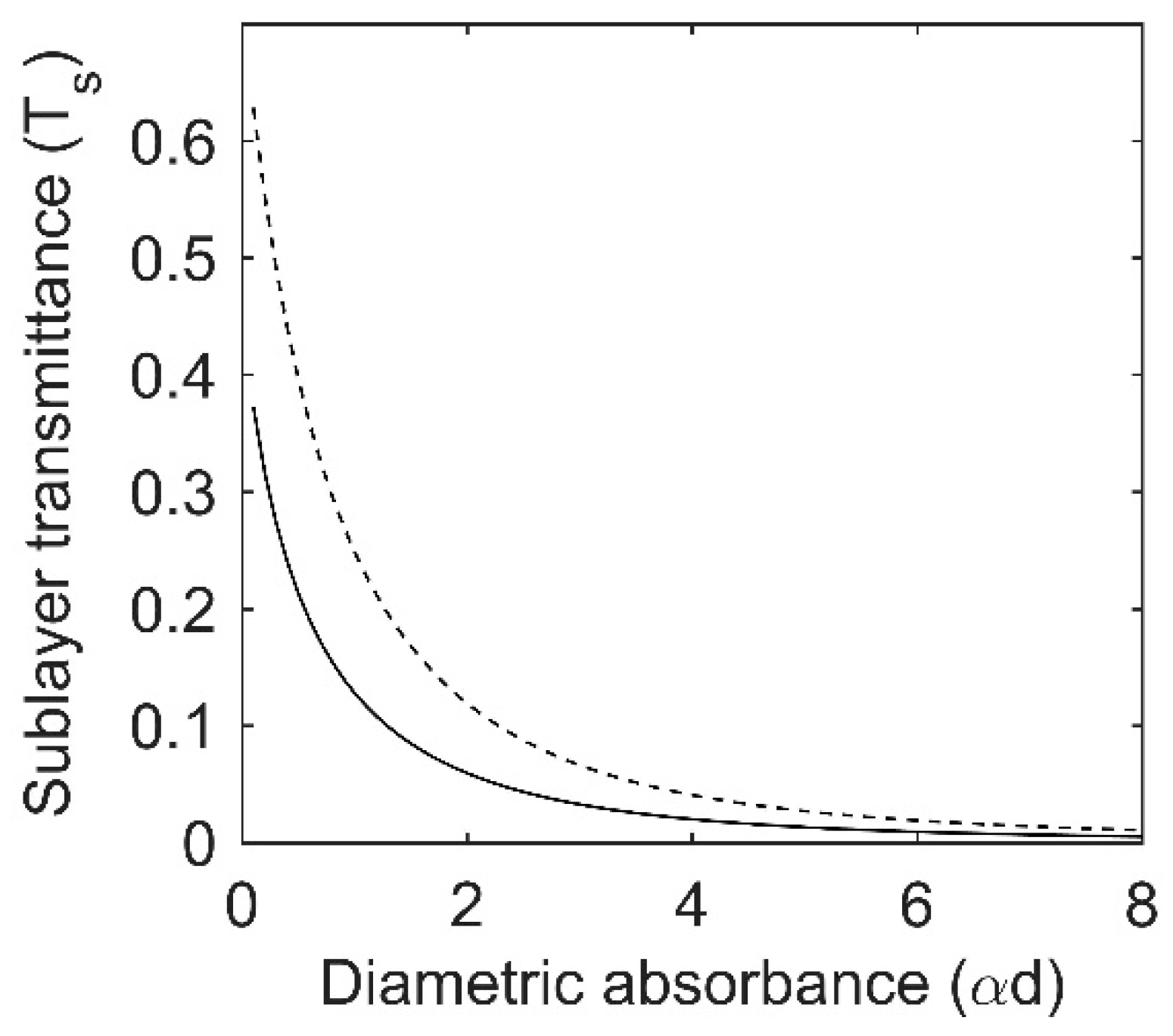
The sublayer transmittances calculated using two equations above are supposed to be equal to each other. Since , and are determined by four parameters (see Nomenclature): the relative refractive index , the particle backscattering ratio , the particle forward scattering ratio and the diametrical absorbance , both in Equations (10) and (11) can be represented as a function of these four parameters i.e., . We set to fixed values of 1.45, 0.2, 0.6 respectively, thus becomes a function of the diametrical absorbance . As shown in Figure 2, the sublayer transmittance of original LIBERTY is underestimated by contrast with theoretical values. This discrepancy can be attributed to the invalid equation of .
2.3. The Fraction of Incident Radiation Entering the Sublayer is Overestimated
In LIBERTY, the fraction of incident radiation entered into the first sublayer is assumed to be (Component 1 in Figure 1); we can change the form into:
where denotes the sublayer attenuation ratio since the sublayer backscattering ratio is equal to the forward scattering ratio. The attenuated part has been added to the radiation penetrated into the particle. Even if Component 1 is correct, the following reflections on the lateral particles (Components 6, 9, 12) will be the same. However, when the reflected radiation by underlying particle bulk strikes on the lateral particles, the reflectance turns into . As mentioned in Section 2.1, LIBERTY may have special treatment for incident radiation since it is collimated rather than scattered radiation. However, this cannot explain the overestimated radiation component in the equation above.
3. Limitations of LIBERTY
3.1. The Directional Changes of Both Particle and Sublayer Scattering Ratios Were Not Considered
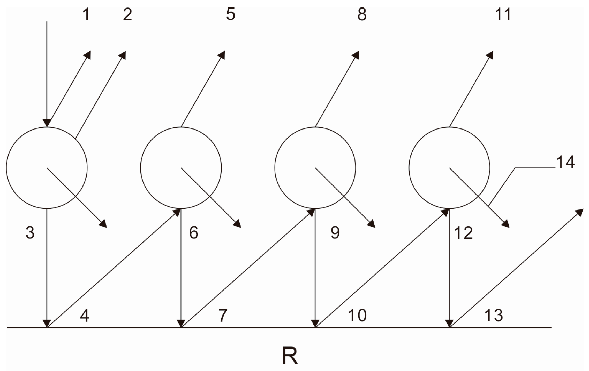
One of the limitations that exists in LIBERTY is that the directional changes of the scattering ratios in both particle and sublayer scales are not considered. If the particle is homogeneous, its backward, lateral and forward scattering ratios (, and ) will be vectors whose directions depend on that of incident radiation. Figure 3 gives a more intuitive representation. Since the sublayer backscattering ratio is related to , and (see Nomenclature), the direction of will be determined by that of incident radiation as well. However, in LIBERTY the direction of is fixed upward. As noted in Figure 1 in reddish tone, is used in Component 2, 5, 8, 11. However, Component 1 is different from Components 5, 8, and 11 because the radiation is incident from above while for Components 5, 8, and 11 the radiation is from below.
3.2. The Radiation Components Were Not Treated Satisfactorily
Several radiation components in Figure 1 need proper treatment. The first is Component 1. As mentioned in Section 2.3, the original Melamed theory assumes that there is of incident radiation reflected on particle surface; the remaining part will propagate into the particle. First let us review the definition of . It represents the backward fraction of outgoing radiation from a sublayer. Figure 4 shows a more intuitive representation. Radiation is incident on the left particle (the entrance particle) from above, and the radiation outgoing from this particle is assumed to be a unit, out of which will propagate to lateral particles, and repeat the same transfer process. Reflections on the adjacent particle surface are not considered, because in real scenarios cells are connected with each other by cell walls, so intercellular radiation will penetrate entirely into cells by multiple reflections between the cell walls. Apparently, takes account of influences of the lateral particles in the same sublayer. The final equation of is:
Melamed [4] assumes at low absorption coefficients where . Hence, the sublayer backscattering and forward scattering ratios are equal to each other. There will be of incident radiation reflected on the particle surface because “the reflected component of the external incident ray is scattered over an angle steradians therefore is zero and is twice the radiation which emerges from within a cell” [3]. However, the reason does not hold. As shown in Figure 4, for the middle particle which receives of outgoing radiation from the left particle, the scattering still happens over an angle of steradians. In addition, since has considered the shadowing of the lateral particles, as explained in Equation (12), the attenuated part has been added into the radiation penetrating into the particle. Obviously, does not conform to the reality. Then, how much incident radiation enters the particle on which it strikes? We believe there is no need to consider the scattering and shadowing of the lateral particles when calculating the penetrated part of incident radiation. Therefore, there will be just of incident radiation reflected on the surface and entering into the particle.
The second radiation component is Component 3. Dawson, Curran and Plummer [3] assume that the sublayer backscattering ratio is , therefore there will be of radiation scattered forward. However, according to the definition of , the shadowing of the lateral particles has been considered, which means a fraction of the total radiation will be attenuated inside the sublayer during radiation transfer. In Figure 4, the radiation transferred into the middle particle is , out of which will be attenuated in this particle ( is the transmittance of a particle). The attenuation will also happen in the right particle, and has included this attenuated radiation. If the particle forward scattering ratio is equal to , then there will be of radiation scattered forward by the sublayer.
3.3. The Morphology of Needle Leaves Was Not Included
LIBERTY is developed to model optical properties of needle leaves but it does not include the morphological structures of needle leaves which makes them different from broadleaves. Needles are narrow and thick, and needle structures with adaxial and abaxial surfaces are neither parallel nor necessarily flat planes [9]. Figure 5 shows an anatomical structure of a typical needle. The limited boundary of single particle sublayer has not been considered in LIBERTY. The number of particles in a sublayer is assumed to be infinite in LIBERTY. Actually, if the boundary constraint is not included, the main difference between LIBERTY and PROSPECT is the sublayer morphology. The sublayer in LIBERTY is composed of compact particles while in PROSPECT it is a flat plate. The two global reflectance calculation methods—Benford theory and Stokes theory, used by LIBERTY and PROSPECT respectively—are essentially the same.
4. Improved Version of LIBERTY
Based on the issues raised above associated with LIBERTY, this section will propose an improved version of LIBERTY, which is called LIBERTYim for convenience.
4.1. Reassessment of the Sublayer Backscattering and Forward Scattering Ratios
In LIBERTY, the particle backscattering ratio is assumed to be equal to the particle forward scattering ratio . However, the prerequisite of this assumption, that is , does not always hold (please refer to Table 1). Hence, the and are not necessarily equal to each other in LIBERTY. As a result, the particle forward scattering ratio must be input into the model as an additional parameter and the sublayer backscattering and forward scattering ratios are not necessarily equal to each other either. The sublayer backscattering and forward scattering ratios are denoted as and in LIBERTYim.
As explained in Section 3.1, it is more reasonable to consider the directional changes of the sublayer backscattering and forward scattering ratios (as shown in Figure 3). When the directions of the particle scattering ratios (i.e., , and ) are taken into account, the calculations of the sublayer scattering ratios are similar to Figure 6. Radiation enters the sublayer through the left particle, which is called the entrance particle. For the middle particle, the incident radiation comes from the left, that is . When the directions of the particle scattering ratios change, the proportions of scattered radiation received by the lateral particles change as well since the receptors for and are sublayers (see Figure A1a,b). We define two direction change coefficients and to represent the proportions of () and received by lateral particles when the directions of particle scattering ratios change. The laterally scattered radiations (the middle and right particles in Figure 6) are assumed to undergo a similar transfer process, so they have been put together. The reassessed value for the sublayer backscattering ratio can be derived by an infinite series summation that converges to:
In the equation above, a transformation is used: . Similarly, the sublayer forward scattering ratio can be calculated by following equation:
Then to and to ratios denote the contributions of the entrance particle to the sublayer backscattering and forward scattering ratios, respectively. When considering the direction changes of particle scattering ratios, and are exactly the first left items on the right-hand side of Equations (14) and (15). Thus, the second left items are same and represent the contributions of the lateral particles to sublayer backscattering and forward scattering ratios.
4.2. Reassessment of the Sublayer Reflectance and Transmittance
The sublayer backscattering ratio and forward scattering ratio do not include the reflection and transmission on the surface of the entrance particle (i.e., rthe left particle in Figure 6). After we get the formulae of and , the equation of sublayer reflectance and transmittance can be derived by:
Stokes theory instead of Benford theory is used to calculate the global reflectance and transmittance. The philosophy of Benford theory is to break down thickness into fractional part ranging from 1 to 2 and the remaining integer part. Actually, the difference in reflectance calculated from these two theories is so tiny that it can be neglected (results not shown). This is due to the same premise on which these two theories are built as mentioned in Section 2.1. Compared with Benford theory, Stokes theory is simpler. The global reflectance and transmittance of homogeneous layers are:
where, , , .
4.3. The Reflectance and Transmittance of a Particle String
It is difficult to consider boundary constraints for a sublayer. We just give the solution of a particle string.
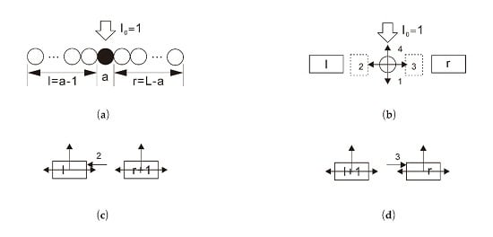
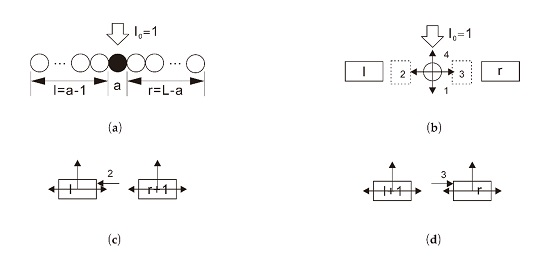
Suppose a limited number (M+N) of particles are arranged compactly in a straight line and unit light is incident isotropically from the left of the system (shown in Figure 7a). Since the system is composed of particles with the same and homogeneous quality, we can regard the M particles as a block and remaining N particles as another block (shown in Figure 7b). If the particle scattering ratios (i.e., , and ) are constants, amd can be treated as the sublayer reflectance and transmittance, thus the global backscattering ratio (U) and forward scattering ratio (D) of the particle string can be calculated by Equation (18). Specific equations are given in Nomenclature.
In order to get the equation of lateral scattering ratio, we list three directional fractions of the nth transfer in Table 2. The total laterally-scattered radiation equals the sum of the “Next” column.
and are the backscattering and forward scattering ratios of the particle string, respectively. and are the reflectance and transmittance of the particle string, respectively. is equal to theoretically. We finally obtain:
If the radiation source is switched to the right of the system, the subscript M and N in Equation (20) will be replaced with each other but remains the same.
From the two equations above, we can obtain:
where equations of and can be found in Nomenclature. Since this is one-dimension case, we need to reassess the directional change coefficients for particle backscattering ratio and lateral scattering ratio , they are denoted as and (see Appendix A). If , then , , .Directional change coefficients for two-dimension case ( and ) instead of and are used to calculate because we need to exclude part of the laterally-scattered radiation. After taking , and into Equation (22) we can get the form of .
Now, let us consider the case in which the direction of incident radiation is perpendicular to the length of the particle string. Suppose there are particles in the string, light is incident on the th left particle (Figure 8a). The substring left to this particle can be regarded as a block, the substring right to this particle can be regarded as another block (Figure 8b). When studying the radiation transfer within the particle string, only Components 2 and 3 need to be considered. Figure 8c,d give a simplified graph of radiation transfer within the particle string for these two components respectively. The reflectance for Component 2 and 3 can be derived like , actually, we just need to replace with in Equation (20).
where and denote the numbers of particles to the left and right of the entrance particle, respectively and their values can be found in Figure 8a. Equations of and can be found in Nomenclature. Therefore, the final equation for global reflectance is:
The global transmittance is:
Six parameters are required to calculate the reflectance and transmittance of a particle string: total number of particles, location of the entrance particle, the refractive index, the diametrical absorbance, the particle backscattering and forward scattering ratios. If the location of the entrance particle moves from left to right in Figure 8a, we will first observe an increase of reflectance, then the reflectance reaches a plateau followed by a decline (Figure 9). The transmittance shows the same pattern. In this study, we select the plateau values as the final reflectance and transmittance.
4.4. Differences between LIBERTY and PROSPECT
The mechanisms of the forward simulation of LIBERTY and PROSPECT are shown in Figure 10. The comparisons between these two models are listed in Table 3. Despite the various chemical constituents which are measured in different bases, there is no substantial difference between these two models. Both models are built on a multiple plate model since their methods to calculate the global reflectance and transmittance (Benford theory and Stokes theory) are essentially the same. The main difference between LIBERTY and PROSPECT is the sublayer morphology. The sublayer is a flat plate in PROSPECT while in LIBERTY it is composed of compact particles. The distinct sublayer morphologies result in different methods to calculate the sublayer reflectance and transmittance. When calculating the sublayer transmittance, LIBERTY uses an indirect method. It first calculates the infinite reflectance which is then used to obtain the sublayer reflectance together with the sublayer transmittance.
For LIBERTY, the input biochemical parameters, the particle diameter and the calibrated absorption coefficients can be incorporated into one parameter: the diametrical absorbance (Figure 10a), which is equivalent to the parameter (Figure 10b) in PROSPECT. However, the difference between and is that can be eliminated in because the contents of biochemical constituents can be measured in area basis for broadleaves. The detailed explanations are given as follows: According to Beer–Lambert law, the absorbance would be dimensionless, which means the unit of would be cm−1 if the unit of is cm. is the linear combination of the contents of the volumetric biochemical constituents (g∙cm−3) and their corresponding absorption coefficients (cm−2·g).
However, the input biochemical constituents are area-based, i.e., rthe unit is g∙cm−2. If the leaf thickness is D (unit cm), the volume-based biochemical constituents can be expressed as a function of area-based biochemical constituents () and D:
After taking Equation (28) into Equation (27), we can get:
where N is the number of sublayers. Actually, the particle diameter in can also be eliminated using the method above. But unlike broadleaves, the biochemical constituents of needle leaves cannot be expressed in area basis since needle leaves are not necessarily flat and the area of a needle leaf is difficult to measure. Area-based biochemical constituents of needle leaves only can be measured using projected area like Di Vittorio [10].
5. Materials and Methods
5.1. Ranges of Input Parameters
To conduct sensitivity analysis and inter-model comparisons, ranges of input parameters would be determined so as to represent more genuine physical and biochemical realities. There are five input parameters in this study: the relative refractive index , the particle backscattering ratio , the particle forward scattering ratio , the diametrical absorbance and the structural parameter . The biochemical constituents such as leaf chlorophyll content, leaf water content, lignin/cellulose content and nitrogen content have been incorporated into ; we did not consider the changes of specific biochemical constituents because: (1) the main limitations of LIBERTY exist in physical rather than biochemical aspects; (2) It is more easy to compare LIBERTY with other models such as PROSPECT which define different sets of biochemical components in various units.
The ranges of the refractive index n and diametrical absorbance were determined by the leaf optical properties model PROSPECT. PROSPECT was built by Jacquemoud and Baret [11], whereafter it underwent several improvements including recalibrations of refractive index and specific absorption coefficients [12]. In this study, the improved version PROSPECT5 was used (the source code can be downloaded from here). In order to get the ranges of the diametrical absorbance , we first calculate the absorption coefficient of one elementary layer which is a linear combination of the content of leaf constituents and their corresponding specific absorption coefficients :
where is the structural parameter, and was taken from PROSPECT5 while and were read from the LOPEX93 dataset, which was downloaded from here. A description of this dataset can be found here. The range of the diametrical absorbance is . The range of structural parameter can be read from this dataset as well.
The determination of the range is more difficult. According to the study of Mandelis, Boroumand and Bergh [7], the value of would lie in [0.1, 0.4]. Simonot, et al. [13] also calculated the particle backscattering ratio using ray tracing technique and found the value is in the range 0.25–0.35. However, in their study, all upper hemispherical fluxes were counted as backscattered radiation which thus included part of the laterally-scattered radiation. In this study, we assume is located in [0, 0.5]. A statistic summary of parameter ranges is listed in Table 1.
5.2. Sensitivity Analysis
Sensitivity analysis (SA) helps to figure out contributions of variability in input parameters to the global variability in model outputs. It has been widely used in mathematical models with complicated input parameters. Generally, there are two types of SA: local SA and global SA. Their major difference is whether consider the interactions between model parameters. In global SA, both individual parameter and interactions between parameters are supposed to explain the global variability while in local SA, only an individual parameter is considered. The theory of global SA can be found in previous literature such as by Ceccato, et al. [14] and Wang, et al. [15]. Suppose a model needs three input parameters. The total variance can be explained by the variance of single parameter and the variance of interactions between parameters:
where denotes the variance of parameter , is the variance of the interaction between parameters and , and is the variance of the interaction between parameters , and .
The first-order sensitivity index for parameter is defined as the ratio between partial input variance of and the total variance. It represents the percentage of the output variance that is accounted for by input parameter .
The total-order sensitivity index for parameter is defined as the ratio of total partial input variance of (including single parameter and interactions between parameter and other parameters) to the total variance.
The difference between and is the percentage of the output variance that is accounted for by interactive effects of parameter with others.
A Matlab software tool—global sensitivity analysis toolbox (GSAT) [16] was used in this study to perform global sensitivity analysis. The source code can be found here. The original program can only produce samples when input parameters are independent to each other. However, in LIBERTY and are constrained under . In order to meet this special need, we made some modifications over the source code [17,18]. The specific method is to define two new variables and whose values are:
Both and lie in [0, 1]. and are regarded as input parameters instead of and . After samples have been produced, the values of and can be derived by the two equations above. There are two sensitivity analysis methods commonly used in previous literature: the Fourier amplitude sensitivity test (FAST) [19] and the Sobel method [20,21]. The Sobel method was adopted for inter-model comparisons while FAST was used for the sensitivity analysis of the particle string model. A quasi-monte Charlo algorithm is employed by GSAT, which produces two sets of samples: one set for evaluation and the other for replacements of complementary variables. The constraint of cannot be ensured during the replacements.
5.3. Inter-Model Comparisons
The original LIBERTY, PROSPECT5 and our improved version of LIBERTY (LIBERTYim) were compared with each other in this study. Despite the variety of input biochemical constituents, the main difference between LIBERTY and PROSPECT is in their sublayer morphologies (see Section 4.4). The absorbance kd used in PROSPECT is equivalent to the diametrical absorbance in LIBERTY. The comparisons were conducted in three aspects: the sublayer backscattering ratio, the sublayer reflectance and transmittance, the global reflectance and transmittance. Since the numbers of the input parameters for three models are inconsistent (Table 4), the numbers of sensitivity indexes are inconsistent as well. There is no scattering ratio in PROSPECT, so the comparisons of sublayer scattering ratios were conducted only between LIBERTY and LIBERTYim. The particle backscattering ratio was assumed to be equal to the forward scattering ratio in both LIBERTY and LIBERTYim for better comparisons between the two models. As a result, the sublayer backscattering and forward scattering ratios were equal to each other as well. The refractive index is fixed in PROSPECT5, but in this study, it serves as a variable.
6. Results
6.1. Sublayer Scattering Ratios Considering the Directional Changes of the Particle Scattering Ratios
In general, the sensitivity patterns of the sublayer backscattering ratio for LIBERTY and LIBERTYim were similar (Figure 11a). Among three input parameters, the particle backscattering ratio explained the most of the variances of for both models. The second sensitive parameter was the diametrical absorbance . Neither LIBERTY nor LIBERTYim was sensitive to the refractive index and the effects of interactions among parameters were insignificant. Although similar in sensitivity patterns, the sublayer backscattering ratios of LIBERTY and LIBERTYim were quite different in values if the same input parameters were entered (Figure 11b).
6.2. The Sublayer Reflectance and Transmittance
The important factor for the sublayer reflectance and transmittance of all three models was the diametrical absorbance (Figure 12). Neither LIBERTY nor LIBERTYim was sensitive to the refractive index .
The sublayer reflectance of LIBERTYim was more sensitive to the diametrical absorbance but less sensitive to the particle backscattering ratios than LIBERTY. In contrast, the global sensitivity index of the sublayer transmittance to decreased slightly after including the directional changes of the particle scattering ratios and the percentage of output variance explained by interactions among parameters changed negligibly. Sensitivity of the sublayer transmittance to the particle backscattering ratios did not change too much. The sublayer reflectance and transmittance of LIBERTYim had similar patterns of sensitivities to input parameters. Among the three models, PROSPECT needs the least number of parameters to calculate the sublayer reflectance and transmittance (the refractive index n and the diametrical absorbance only). Interactions between these two parameters could explain a great deal of output variance of the sublayer reflectance of PROSPECT. Compared with the sublayer transmittance, the sublayer reflectance of PROSPECT is much more sensitive to the refractive index . The calculated sublayer reflectance and transmittance of LIBERTY and LIBERTYim were quite different if the same input parameters were entered (Figure 13a).
6.3. The Global Reflectance and Transmittance
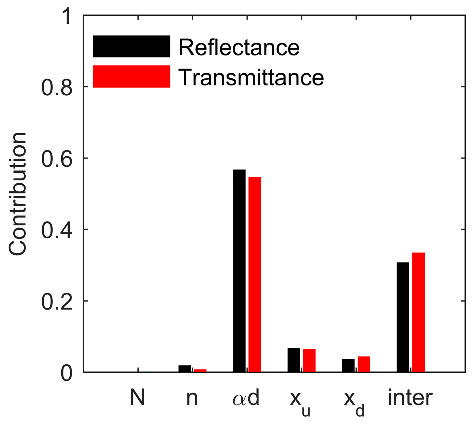
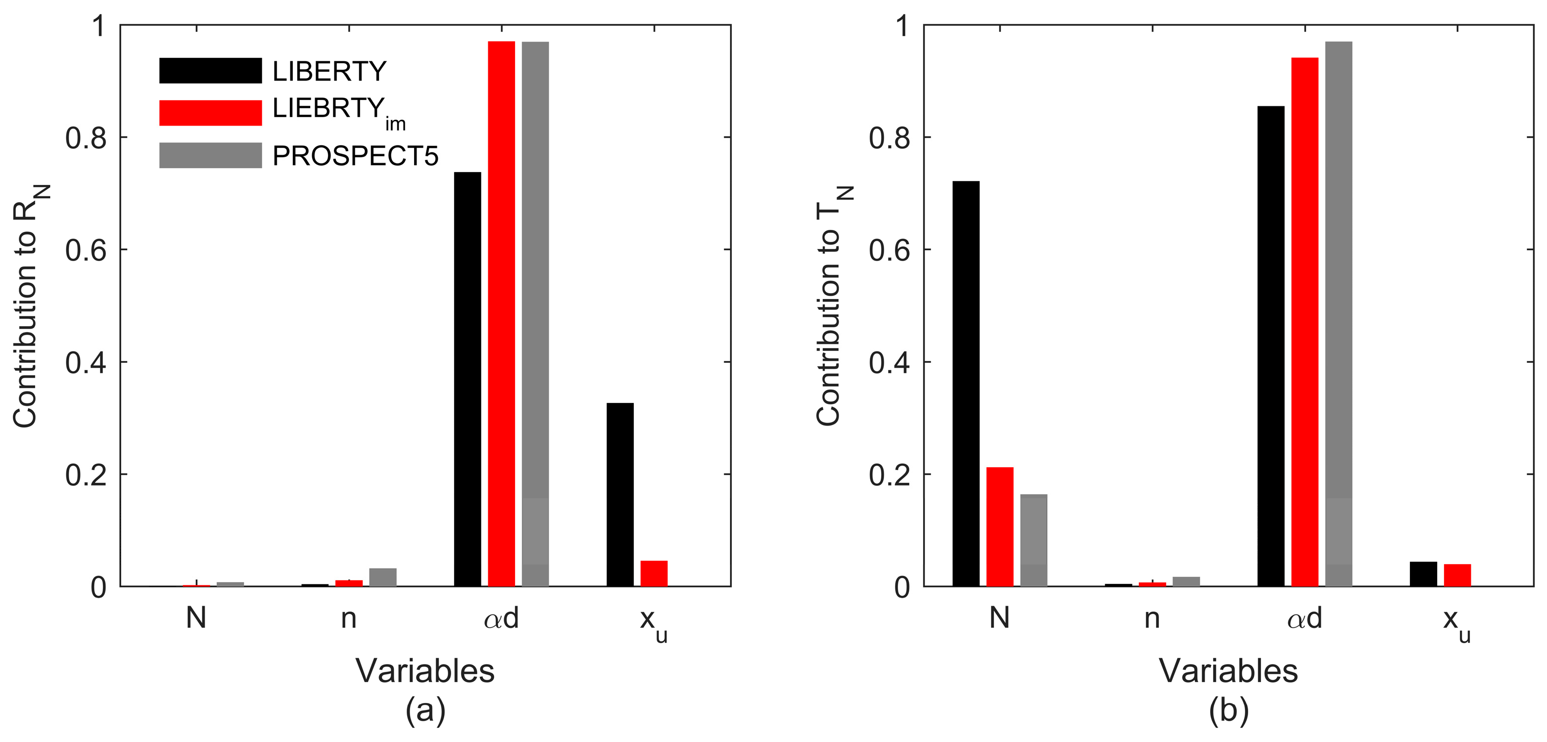
Generally, the diametrical absorbance was the dominant factor contributing to both global reflectance and transmittance of all three models while the refractive index was the insignificant factor (Figure 14). The global reflectance of LIBERTY was sensitive to the particle backscattering ratio while the interactions among input parameters was not very important. Meanwhile, the number of sublayers and the interactions among input parameters played important roles in the output variance of the global transmittance of LIBERTY. For LIBERTYim, the global reflectance was insensitive to other parameters apart from the diametrical absorbance . However, compared with the global reflectance, the global transmittance was much more sensitive to the number of sublayers and the interactions among input parameters. For PROSPECT5, parameters except the diametrical absorbance had little impact on the variance of the global reflectance.
The sensitivity pattern of the global reflectance and transmittance of LIBERTY was quite different from that of PROSPECT. But after being physically corrected, LIBERTY had similar pattern to PROSPECT in simulated global reflectance and transmittance. Considering the directional changes of the scattering ratios witnessed an increased sensitivity of the global reflectance and transmittance to the diametrical absorbance. However, the sensitivities of the global reflectance to the particle backscattering ratio , the number of sublayers and the global transmittance to interactions among parameters decreased sharply. When the same input parameters were entered into LIBERTY and LIBERTYim, great differences in the infinite reflectance, the sublayer and global reflectance and transmittance were observed (Figure 13).
6.4. Reflectance and Transmittance of a Particle String
The differences of sensitivity between the reflectance and transmittance are quite small (see Figure 15). Both of them are most sensitive to the diametrical absorbance followed by the interactions among parameters. Other factors such as the number of particles , the refractive index n, the particle scattering ratios and contribute little to output reflectance and transmittance.
7. Discussion
The directional changes of the particle scattering ratios have great impact on the sublayer backscattering ratios (Figure 11b). The sublayer reflectance and transmittance were calculated based on the sublayer scattering ratios with consideration of the entrance particle. Since the sublayer backscattering ratio and forward scattering ratio were assumed to be equal in this study, the sensitivity differences of the sublayer reflectance and transmittance to input parameters between LIBERTY and LIBERTYim are due to the distinct treatments of the radiation components related to the entrance particle. As explained in Section 4.4, the methods used by LIBERTY and PROSPECT to calculate the global reflectance and transmittance are essentially the same. However, the sensitivity analysis of the global reflectance and transmittance showed different patterns for these two models. By contrast, LIBERTYim has similar sensitivity patterns to PROSPECT with respect to the global reflectance and transmittance. The results demonstrate indirectly the limitations of LIBERTY and the validity of LIBERTYim. The advantage of LIBERTYim is that neither its global reflectance nor transmittance is sensitive to the particle scattering ratios.
Compared with PROSPECT, LIBERTY needs an additional parameter (i.e., the particle backscattering ratio ) to obtain the sublayer reflectance and transmittance, which is determined by its distinct sublayer morphology. The particle forward scattering ratio was assumed to be equal to the particle backscattering ratio . However, the condition for this equality (i.e., ) does not always hold (see Table 1), indicating independence of . Thus, would be entered into LIBERTY as an input parameter under the constraint of . The introductions of the additional parameters will result in more uncertainties. Actually, the sublayer scattering ratios and the diametrical absorbance are related with each other in an unknown fashion. Once their relationship can be determined by mathematical equations, LIBERTY will have fewer parameters. The main limitation of LIBERTY is the assumption that the sublayer is infinite extending. Needle leaves are narrow and thin, hence, they cannot be regarded as endless in width. If the boundary constraints of needle leaves are not considered, LIBERTY is more suitable for modelling the optical properties of broadleaves instead of needle leaves.
In this study, we worked out the reflectance and transmittance of a particle string, which is a theoretical model. The particle string model may be capable of modelling leaf optical properties for needle leaves. If the model is used for this purpose, the particle in this model will no longer denote the cell anymore; the whole needle is regarded as a particle string. The greatest advantage of this particle string model is the inclusion of the special morphology of needle leaves. The equivalent diameter of particle can be calculated using measured thickness and width. The particle number can be assumed to be infinite since the needle leaf is long enough, thus the number of particles N can be eliminated. There are only four parameters left: refractive index , diametrical absorbance , particle backscattering and forward scattering ratios ( and ). and can be treated as parameters controlling the anatomical morphology of needle leaves. However, there are several issues need to be addressed if the particle string model can be used. Firstly, the absorption coefficients may not reflect chemical reality, it is just a calibrated parameter used in the model, but this does not matter since the ultimate goals are to simulate the reflectance and transmittance and to estimate biochemical concentrations. The intermediate products such as absorption coefficients will not affect the performance of the model. Secondly, and are related to and . If we regard the particle scattering ratios and the diametrical absorbance as independent variables, the physical reality of the particle scattering is violated. However, it seems hard to determine their relationships. Once their relations can be expressed precisely by mathematical equations, the parameters and can be eliminated. There are two parameters left: refractive index and diametrical absorbance . Anatomical morphology of needle leaves can be controlled by diametrical absorbance . Thus the parsimony of this model needs to be checked. Lastly, the particle ignores the intercellular air spaces inside the needle leaves. LIBERTY describes the intercellular organizations inside the leaf in a more delicate manner than PROSPECT. However, it cannot be used to model optical properties for needle leaves. Both LIBERTY and PROSPECT has considered intercellular air spaces. To include intercellular air spaces into the particle string model, differences between broadleaves and needle leaves would be noticed. Although this model is theoretically capable of modeling optical properties for needle leaves, experiments are needed to test its applicability.
8. Conclusions
Our study pointed out several limitations existing in LIBERTY according to clues of these limitations. Based on the findings, theoretical improvements of LIBERTY were given. The improved version of LIBERTY (LIBERTYim) has limited differences to PROSPECT except in their distinct sublayer morphologies. Unless the special realities of needle leaves (boundary constraints) are included, LIBERTY cannot be truly used for modelling optical properties for needle leaves. However, it is difficult to introduce the boundary constraints into a sublayer in which a particle denotes a cell. However, the reflectance and transmittance of a string composed limited number of particles can be calculated. We worked out the reflectance and transmittance of a particle string which is composed of a limited number of particles. The particle string model has great potential for needle leaf optical properties modelling. It includes leaf morphology and radiation scattered in all directions around the needle leaves can be calculated using this particle string. However, delicate experiments are needed to test the theory.
Acknowledgments
This research was supported by key research and development programs for global change and adaptation (2016YFA0600202), National Natural Science Foundation of China (41671343, 41371070). We hereby express our sincere gratitude to Dr. Stéphane Jacquemoud of iPGP(INSTITUT DE PHYSIQUE DU GLOBE DE PARIS) for providing LOPEX93 dataset.
Author Contributions
Jun Wang carried out the research and wrote the paper under the guidance of Weimin Ju.
Conflicts of Interest
The authors declare no conflict of interest.
Nomenclature
| Notations | Connotations | Equations |
| Structural parameter, representing the number of sublayers. | Serves as a variable | |
| Relative refractive index (internal to external refractive index ratio if the external media has a lower refractive index) | Serves as a variable | |
| Absorption coefficient | Serves as a variable | |
| Particle diameter | Serves as a variable | |
| Diametrical absorbance | Serves as a variable | |
| Particle backscattering ratio | Serves as a variable | |
| Particle forward scattering ratio | Serves as a variable | |
| Particle lateral scattering ratio | ||
| Directional change coefficient of and for a sublayer | Constant, | |
| Directional change coefficient of for a sublayer | Constant, | |
| Directional change coefficient of and for a particle string | Constant, | |
| Directional change coefficient of for a particle string | Constant, | |
| External reflection coefficient for direction (supposing the external media has a lower refractive index) | where | |
| External reflectance (supposing the external media has a lower refractive index) | ||
| Internal reflectance (supposing the external media has a lower refractive index) | where | |
| One-pass transmittance inside the particle | ||
| Particle transmittance | ||
| Sublayer backscattering ratio, neglecting the directional changes of the particle scattering ratios (, and ) | ||
| Sublayer backscattering ratio, considering the directional changes of the particle scattering ratios (, and ) | Original version: Improved version: | |
| Sublayer backscattering ratio, considering the directional changes of the particle scattering ratios (, and ) | Original version: Improved version: | |
| Sublayer reflectance | Original version: Improved version: | |
| Sublayer transmittance | Original version: Improved version: | |
| Global reflectance of N homogenous layers | Where , , | |
| Global transmittance of N homogenous layers | ||
| Backscattering ratio of a particle string composed of particles, the light is assumed to incident along the string length | Where , | |
| Forward scattering ratio of a particle string composed of particles, the light is assumed to incident along the string length |
Appendix A
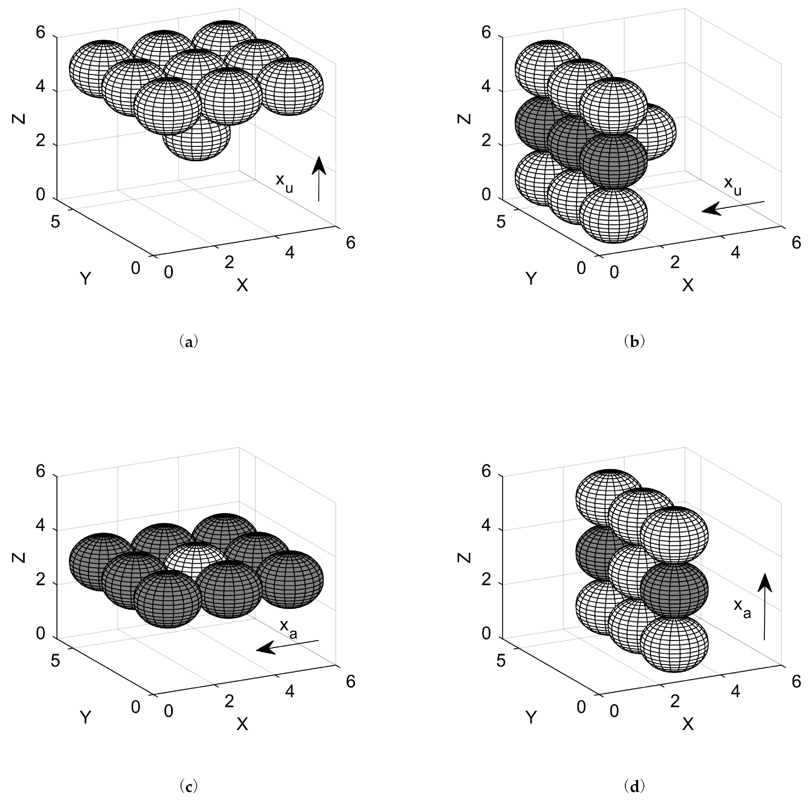
, and are the particle backscattering, lateral scattering and forward scattering ratio, respectively. When the incident radiation changes direction, , and would change directions as well (see Section 4.1). However, and orient to a plane while orients to surrounding particles in the same sublayer. As shown in Figure A1, when directs upward along Z axis, the receptor is the upward sublayer (Figure A1a), When its direction changes (along X axis), only part of will be received by adjacent particles (grey balls in Figure A1b), the remaining part will go upward and downward. The part of received by adjacent particles is termed the direction change coefficient, denoted as . For , the influences of direction change is a bit different since it directs to adjacent particles (Figure A1c,d). In order to calculate , we just need to calculate the projection area of receptors to the emitting particle surface.
Figure A1.
Influences of direction changes on the particle backscattering ratio and lateral scattering ratio . (a) when directs upward; (b) when directs laterally; (c) when directs laterally; (d) when directs upward. The radiation comes out from the central particle in the cube. The aggregation of particles in XOY is a sublayer. Grey balls are lateral particles in the same sublayer.

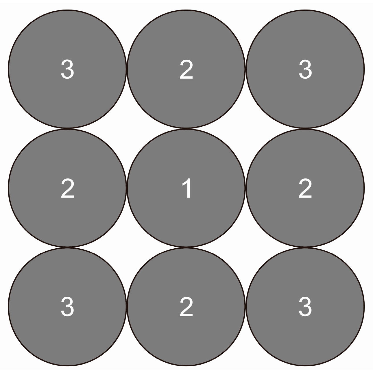
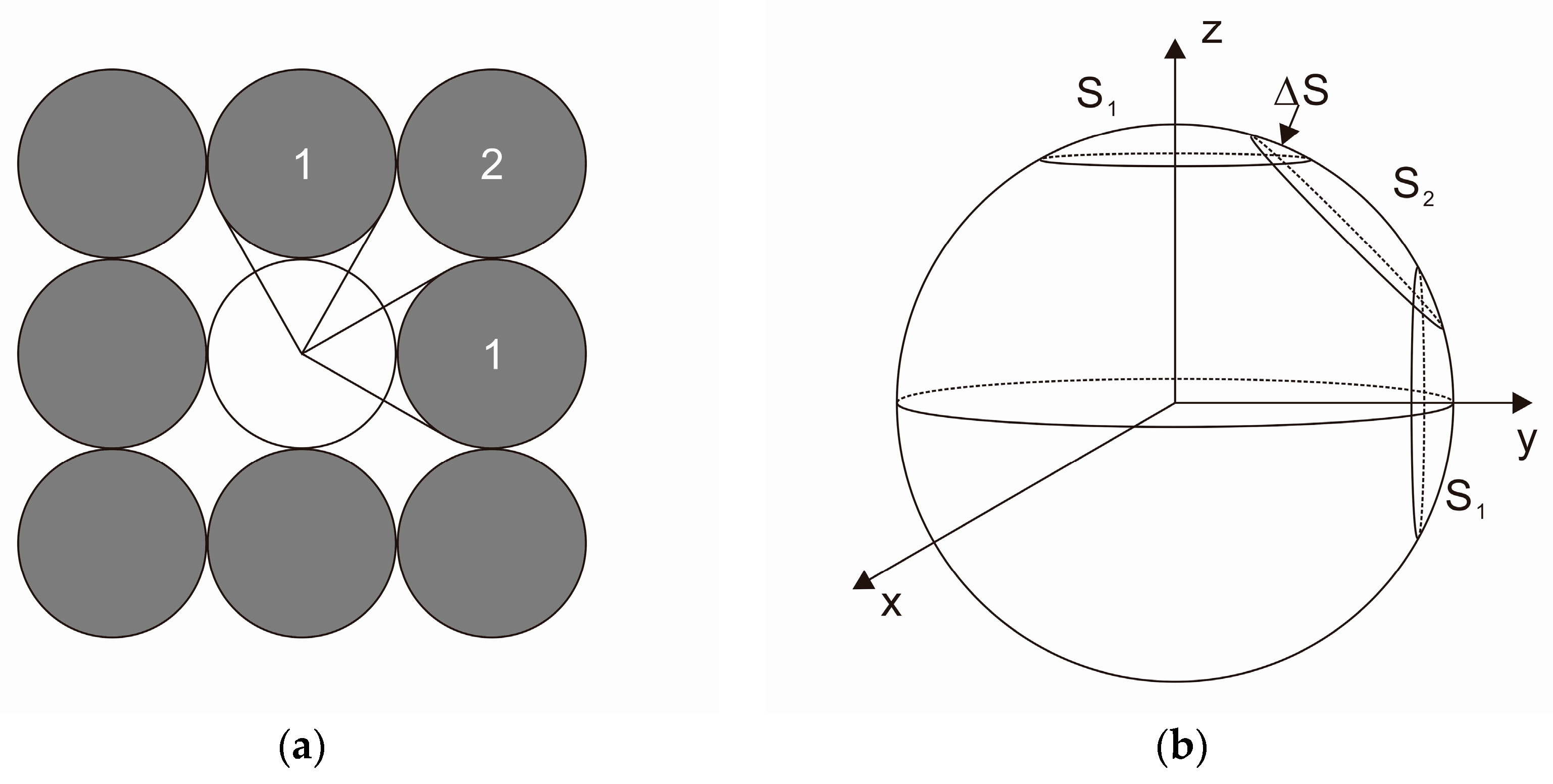
First, let us calculate the direction change coefficient for . Theoretically, the radiation directing toward adjacent particles would be homogeneous. Therefore, we need to get the total projections area of receptors to the emitting particle. As shown in Figure A2a, the size of projection area depends on the distance between particles. The projection areas on the emitting particle are displayed in Figure A2b. and are the projection areas for Particle 1 and 2 in Figure A2a, respectively. is the overlapping area of and . , and can be worked out using solid geometry. Suppose the particle radius is 1, then,
Therefore, the direction change coefficient for is
The direction change coefficients for and are the same and can be calculated like . A 2-D sketch of receptors for and is displayed in Figure A3. The projection areas of particles numbered as 1 and 2 are exactly same as Figure A2a. For the receptor numbered as 3, its projection area to the emitting particle can be regarded as the remaining part of the particle surface in a quadrant, that is . Therefore, the direction change coefficient for and is:
Figure A2.
Schematic representation of receptors (grey circles) for the particle lateral scattering ratio . (a) 2-Dimension sketch of receptors (grey circles) and emitting particle (white circle); (b) projection areas for the numbered particles in (a), is the projection area for Particle 1, is the projection area for Particle 2, is the overlapping area.

Figure A3.
2-Dimension sketch of receptors (grey circles) for the particle backscattering ratio or forward scattering ratio .
Figure A3.
2-Dimension sketch of receptors (grey circles) for the particle backscattering ratio or forward scattering ratio .
References
- Wang, L.; Wang, W.; Dorsey, J.; Yang, X.; Guo, B.; Shum, H.-Y. Real-time rendering of plant leaves. In ACM SIGGRAPH 2006 Courses; ACM: Boston, MA, USA, 2006; p. 5. [Google Scholar]
- Jacquemoud, S.; Ustin, L. Modeling leaf optical properties. In Photobiological Sciences Online; American Society for Photobiology: McLean, VA, USA, 2008. [Google Scholar]
- Dawson, T.P.; Curran, P.J.; Plummer, S.E. LIBERTY—Modeling the effects of leaf biochemical concentration on reflectance spectra. Remote Sens. Environ. 1998, 65, 50–60. [Google Scholar] [CrossRef]
- Melamed, N.T. Optical properties of powders. Part I. Optical absorption coefficients and the absolute value of the diffuse reflectance. Part II. Properties of luminescent powders. J. Appl. Phys. 1963, 34, 560–570. [Google Scholar] [CrossRef]
- Benford, F. Radiation in a diffusing medium. J. Opt. Soc. Am. 1946, 36, 524. [Google Scholar] [CrossRef] [PubMed]
- Moorthy, I.; Miller, J.R.; Noland, T.L. Estimating chlorophyll concentration in conifer needles with hyperspectral data: An assessment at the needle and canopy level. Remote Sens. Environ. 2008, 112, 2824–2838. [Google Scholar] [CrossRef]
- Mandelis, A.; Boroumand, F.; Bergh, H.V. Quantitative diffuse reflectance spectroscopy of large powders: The melamed model revisited. Appl. Opt. 1990, 29, 2853–2860. [Google Scholar] [CrossRef] [PubMed]
- Stokes, G.G. On the intensity of the light reflected from or transmitted through a pile of plates. Proc. R. Soc. Lond. 1860, 11, 545–556. [Google Scholar] [CrossRef]
- Zhang, Y.; Chen, J.M.; Miller, J.R.; Noland, T.L. Retrieving chlorophyll content in conifer needles from hyperspectral measurements. Can. J. Remote. Sens. 2008, 34, 296–310. [Google Scholar]
- Di Vittorio, A.V. Enhancing a leaf radiative transfer model to estimate concentrations and in vivo specific absorption coefficients of total carotenoids and chlorophylls a and b from single-needle reflectance and transmittance. Remote Sens. Environ. 2009, 113, 1948–1966. [Google Scholar] [CrossRef]
- Jacquemoud, S.; Baret, F. Prospect: A model of leaf optical-properties spectra. Remote Sens. Environ. 1990, 34, 75–91. [Google Scholar] [CrossRef]
- Feret, J.-B.; François, C.; Asner, G.P.; Gitelson, A.A.; Martin, R.E.; Bidel, L.P.; Ustin, S.L.; le Maire, G.; Jacquemoud, S. Prospect-4 and 5: Advances in the leaf optical properties model separating photosynthetic pigments. Remote Sens. Environ. 2008, 112, 3030–3043. [Google Scholar] [CrossRef]
- Simonot, L.; Hébert, M.; Hersch, R.D.; Garay, H. Ray scattering model for spherical transparent particles. J. Opt. Soc. Am. A 2008, 25, 1521–1534. [Google Scholar] [CrossRef]
- Ceccato, P.; Gobron, N.; Flasse, S.; Pinty, B.; Tarantola, S. Designing a spectral index to estimate vegetation water content from remote sensing data: Part 1: Theoretical approach. Remote Sens. Environ. 2002, 82, 188–197. [Google Scholar] [CrossRef]
- Wang, Z.; Skidmore, A.K.; Wang, T.; Darvishzadeh, R.; Hearne, J. Applicability of the prospect model for estimating protein and cellulose+ lignin in fresh leaves. Remote Sens. Environ. 2015, 168, 205–218. [Google Scholar] [CrossRef]
- Cannavó, F. Sensitivity analysis for volcanic source modeling quality assessment and model selection. Comput. Geosci. 2012, 44, 52–59. [Google Scholar] [CrossRef]
- He, W.; Yang, H. Efast method for global sensitivity analysis of remote sensing model’s parameters. Remote Sensing Technol. Appl. 2013, 28, 836–843. [Google Scholar]
- Saltelli, A.; Tarantola, S.; Chan, K.S. A quantitative model-independent method for global sensitivity analysis of model output. Technometrics 1999, 41, 39–56. [Google Scholar] [CrossRef]
- Saltelli, A.; Bolado, R. An alternative way to compute fourier amplitude sensitivity test (fast). Comput. Stat. Data Anal. 1998, 26, 445–460. [Google Scholar] [CrossRef]
- Sobol, I.M. Global sensitivity indices for nonlinear mathematical models and their monte carlo estimates. Math. Comput. Simul. 2001, 55, 271–280. [Google Scholar] [CrossRef]
- Sobol, I.M. On sensitivity estimation for nonlinear mathematical models. Matematicheskoe Modelirovanie 1990, 2, 112–118. [Google Scholar]
Figure 1.
A schematic representation of Melamed theory [3,4]. is the particle backscattering ratio, is the external reflectance, is the transmittance of a particle, is the reflectance of underlying material. Their equations can be found in Nomenclature. The fonts in reddish tone denote the sublayer backscattering ratio used by corresponding components.

Keys to radiative components: 1. ; 2. ; 3. ; 4. ; 5. ; 6. ; 7. ; 8. ; 9. ; 10. ; 11. ; 12. ; 13. ; 14. .
Figure 2.
Sublayer transmittance as a function of diametrical absorbance . is the refractive index, and are the particle backscattering and forward scattering ratios, respectively. They were set to fixed values 1.45, 0.2, 0.6 respectively. Dashed line denotes the theoretical value calculated by Equation (11), solid line is derived using Equation (10).

Figure 3.
The directional changes of particle backscattering, lateral scattering and forward scattering ratios (, and , respectively) with incident radiation. The arrows above indicate the directions of incident radiation.
Figure 3.
The directional changes of particle backscattering, lateral scattering and forward scattering ratios (, and , respectively) with incident radiation. The arrows above indicate the directions of incident radiation.

Figure 4.
A schematic representation of sublayer backscattering ratio (). The total outgoing radiation of the left particle is assumed to be a unit, is the transmittance of particles. This is in accordance with original definition which does not consider the directional change of particle scattering ratios (, and ).
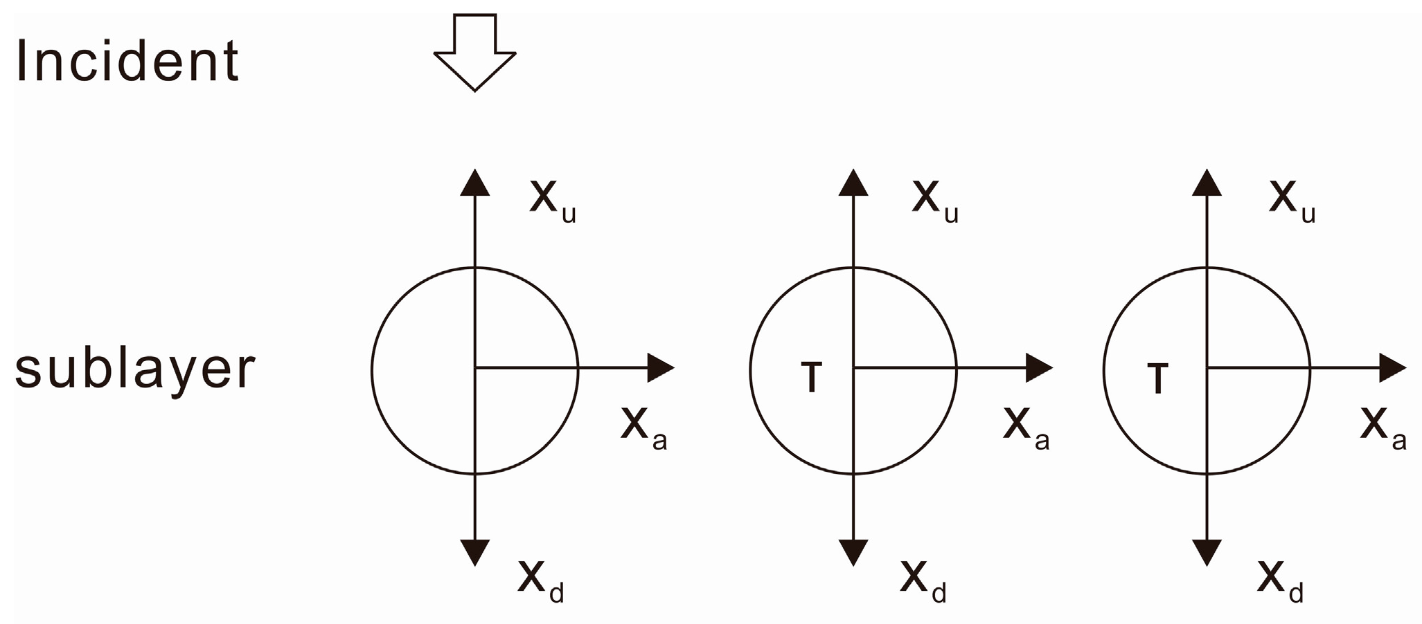
Figure 5.
Photomicrograph of Pinus banksiana needle cross sections. The source is Moorthy, Miller and Noland [6].
Figure 5.
Photomicrograph of Pinus banksiana needle cross sections. The source is Moorthy, Miller and Noland [6].

Figure 6.
A schematic representation of sublayer backscattering and forward scattering with direction changes of particle scattering ratios taken into account. is the particle transmittance. , and represent the particle backscattering, lateral scattering and forward scattering ratios, respectively. and are the directional change coefficients for () and , respectively; their values have been given in Appendix A.
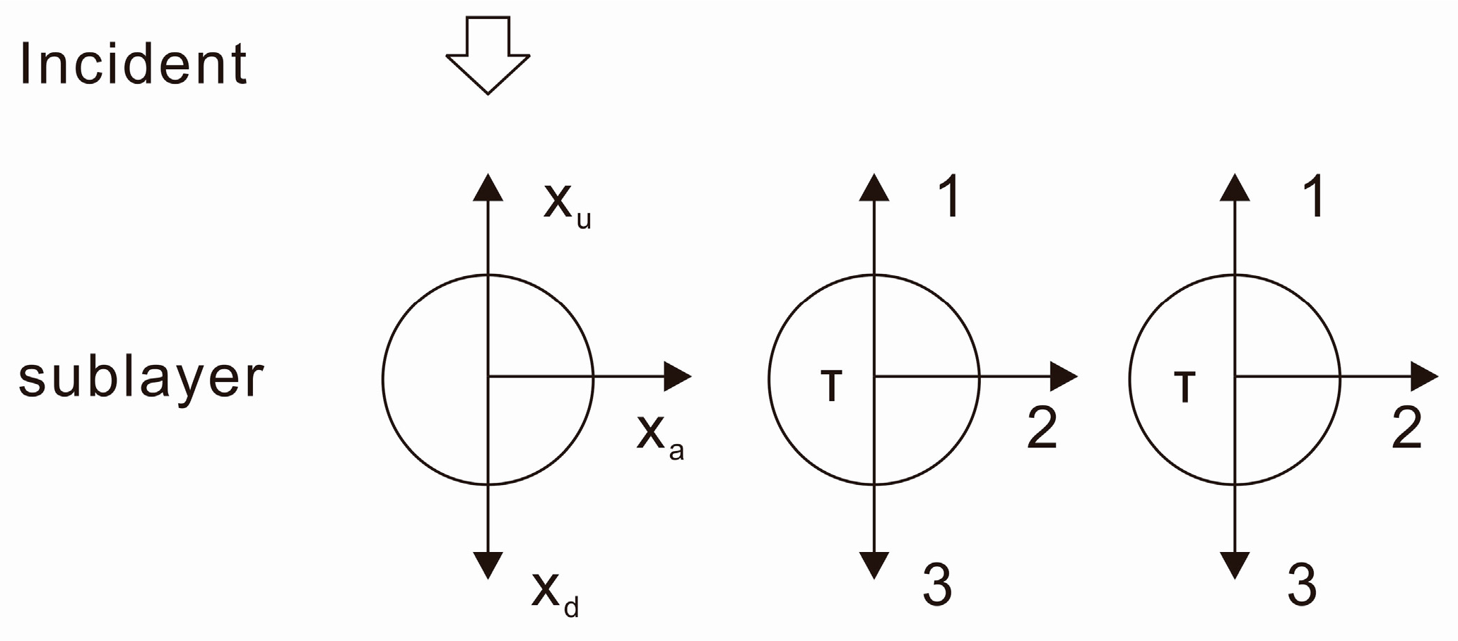
Figure 7.
Schematic graphs of radiation transfer in a particle string. (a) the real situation when light incidents from the left along the string length; (b) a simplified graph of the system when taking M particles as a block and the other N particles as another block. The incident radiation () is assumed to be a unit. and are the backscattering and forward scattering ratios of the particle string, respectively. and are the reflectance and transmittance of the particle string, respectively.
Figure 8.
Schematic graphs of radiation transfer in a particle string when light is incident perpendicularly to the string length (). (a) real situation when unit radiation is incident on the th left particle; (b) simplified graph when taking left particles as a block and right particles as a block; (c) simplified graph of radiation transfer for component 2 in (b); (d) simplified graph of radiation transfer for component 3 in (b). is the incident radiation which is assumed to be a unit.
Figure 9.
A typical relationship between reflectance and transmittance and location of the entrance particle . is the total number of particles, is the refractive index, is the diametrical absorbance, and are the particle backscattering and forward scattering ratios, respectively. All other parameters were set to constants i.e., r.
Figure 10.
Mechanisms of the forward simulation of (a) LIBERTY and (b) PROSPECT5. The definitions of parameters are given in the top of (a).
Figure 10.
Mechanisms of the forward simulation of (a) LIBERTY and (b) PROSPECT5. The definitions of parameters are given in the top of (a).
Figure 11.
Comparisons of the sublayer backscattering ratio between LIBERTY and LIBERTYim. (a) results of Fourier amplitude sensitivity test (FAST) first-order sensitivity coefficients to the sublayer backscattering ratio. n is the relative refractive index, is the diametrical absorbance, is the particle backscattering ratio, inter denotes the interactions. Input parameters for models are listed in Table 4. Their ranges were taken from Table 1; (b) calculated sublayer backscattering ratio for LIBERTY and LIBERTYim with the same input parameters. The particle diameter d, the particle backscattering ratio xu, the number of sublayers N, baseline, the albino absorption, chlorophyll content (% dry matter), water content (% dry matter), lignin and cellulose content (% dry matter) and protein content (% dry matter) were set to 40 μm, 0.045, 1.6, 0.0005 μm−1, 2 mg·g−1, 200 mg·g−1, 100 mg·g−1, 40 mg·g−1 and 1 mg·g−1, respectively.

Figure 12.
Results of global sensitivity coefficients of (a) the sublayer reflectance and (b) the sublayer transmittance to input variables using Sobel method. n is relative refractive index, is diametrical absorbance which is assumed to be equivalent to elementary layer absorbance in PROSPECT, is the particle backscattering ratio, and inter denotes the interactions among parameters. Input parameters for models are listed in Table 4. Their ranges were taken from Table 1. The legend is given in the right barplot.

Figure 13.
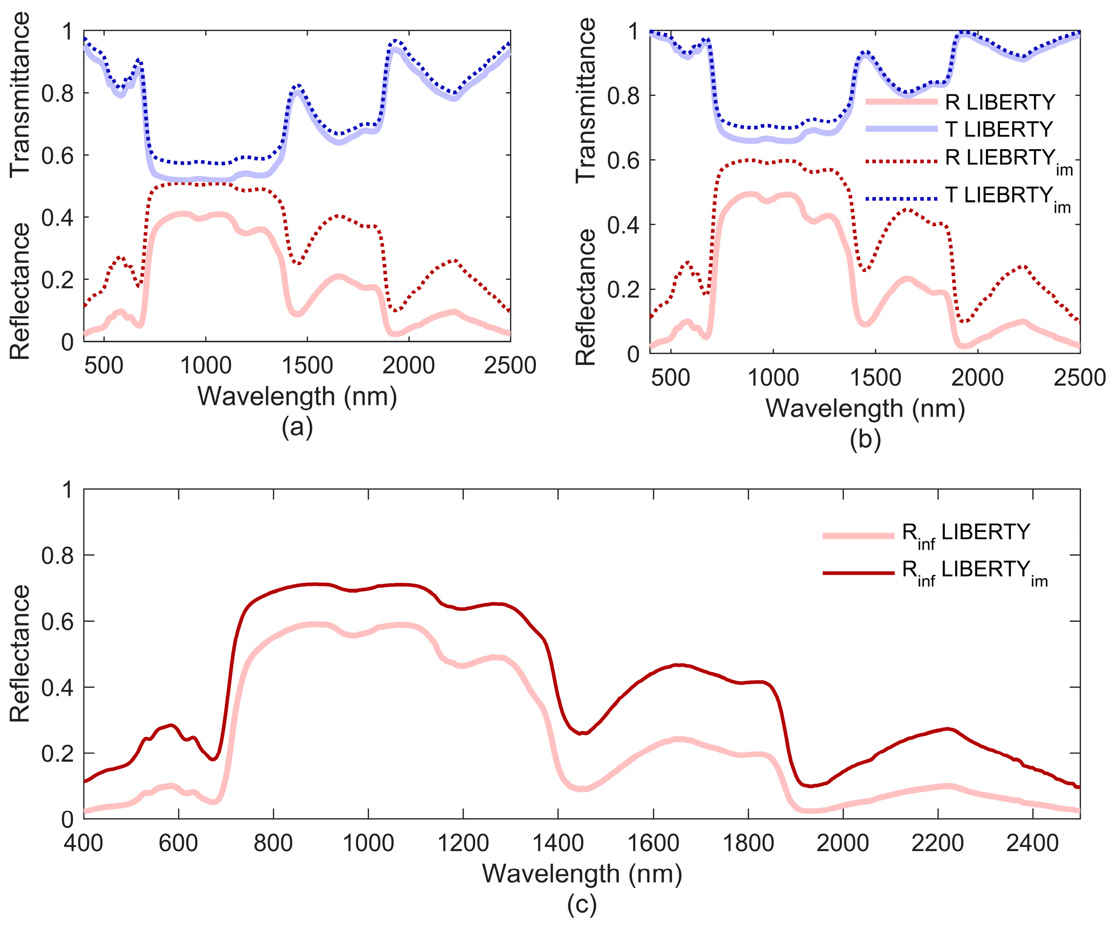
Comparisons of outputs from LIBERTY and LIBERTYim when the same input parameters were entered. (a) the sublayer reflectance and transmittance; (b) global reflectance and transmittance and (c) The infinite reflectance. The legend of (a) is given in (b). The input parameters i.e., rthe particle diameter , the particle backscattering ratio , the number of sublayers , baseline, the albino absorption, chlorophyll content (% dry matter), water content (% dry matter), lignin and cellulose content (% dry matter), protein content (% dry matter) were set to 40 , 0.045, 1.6, 0.0005 , 2 mg∙g−1, 200 mg∙g−1, 100 mg∙g−1, 40 mg∙g−1 and 1 mg∙g−1, respectively. For LIBERTYim, the additional input parameter was set to be equal to .
Figure 13.
Comparisons of outputs from LIBERTY and LIBERTYim when the same input parameters were entered. (a) the sublayer reflectance and transmittance; (b) global reflectance and transmittance and (c) The infinite reflectance. The legend of (a) is given in (b). The input parameters i.e., rthe particle diameter , the particle backscattering ratio , the number of sublayers , baseline, the albino absorption, chlorophyll content (% dry matter), water content (% dry matter), lignin and cellulose content (% dry matter), protein content (% dry matter) were set to 40 , 0.045, 1.6, 0.0005 , 2 mg∙g−1, 200 mg∙g−1, 100 mg∙g−1, 40 mg∙g−1 and 1 mg∙g−1, respectively. For LIBERTYim, the additional input parameter was set to be equal to .

Figure 14.
Results of global sensitivity coefficients of (a) the global reflectance and (b) transmittance to input variables using Sobel method. is the structural parameter, n is the relative refractive index, is the diametrical absorbance which is assumed to be equivalent to elementary layer absorbance in PROSPECT, is the particle backscattering ratio, inter denotes the interactions. Input parameters for models are listed in Table 4. Their ranges were taken from Table 1. The legend is given in the left barplot.

Figure 15.
FAST first order sensitivity coefficients of the reflectance and transmittance of a particle string . is the total number of particles, n is relative refractive index, is diametrical absorbance, and are particle backscattering and forward scattering ratios, inter denotes the interactions.

Table 1.
Ranges of input parameters. is the refractive index, is the diametrical absorbance, is the number of sublayers, is the particle backscattering ratio.
Table 1.
Ranges of input parameters. is the refractive index, is the diametrical absorbance, is the number of sublayers, is the particle backscattering ratio.
| Input Parameters | Minimum Value | Maximum Value |
|---|---|---|
| 1.2708 | 1.5295 | |
| 0.0021 | 8.4985 | |
| 1.0927 | 3 | |
| 0 | 0.5 |
Table 2.
Statistics of three directional fractions of outgoing radiation in the nth radiation transfer in Figure 7b. and are the backscattering and forward scattering ratios of the particle string, respectively. and are the reflectance and transmittance of the particle string, respectively.
Table 2.
Statistics of three directional fractions of outgoing radiation in the nth radiation transfer in Figure 7b. and are the backscattering and forward scattering ratios of the particle string, respectively. and are the reflectance and transmittance of the particle string, respectively.
| Count | Backward * | Forward * | Reflected * | Next ** |
|---|---|---|---|---|
| 1 | ||||
| 2 | ||||
| 3 | ||||
| 4 | ||||
| 5 | ||||
| 6 | ||||
| 7 |
* directions are relative to incident radiation. ** radiations left for next transfer.
Table 3.
Comparisons between Leaf Incorporating Biochemistry Exhibiting Reflectance and Transmittance Yields (LIBERTY) and The optical PROperties SPECTra model (PROSPECT5).
Table 3.
Comparisons between Leaf Incorporating Biochemistry Exhibiting Reflectance and Transmittance Yields (LIBERTY) and The optical PROperties SPECTra model (PROSPECT5).
| PROSPECT5 | LIBERTY | Note | |
|---|---|---|---|
| Number of input parameters | 6 | 9 | |
| Number of input biochemical parameters | 5 | 6 | |
| Number of input structural parameters | 1 | 3 | |
| Incorporated absorbance | kd | Equivalent | |
| Sublayer morphology | Plate model | Compact particle model | |
| Method to calculate global reflectance and transmittance | Stokes theory | Benford theory | Essentially the same |
| Boundary | Not considered | Not considered | same |
| Special treatment of incident radiation | Yes | No |
Table 4.
Inputs for three models *.
| Models | |||
|---|---|---|---|
| LIBERTY | LIBERTYim ** | PROSPECT5 | |
| Outputs | Inputs | ||
| and | |||
| and | |||
| and | |||
* the definitions of the parameters are given in Nomenclature. ** improved LIBERTY in this study.
© 2017 by the authors. Licensee MDPI, Basel, Switzerland. This article is an open access article distributed under the terms and conditions of the Creative Commons Attribution (CC BY) license (http://creativecommons.org/licenses/by/4.0/).
Share and Cite
MDPI and ACS Style
Wang, J.; Ju, W. Limitations and Improvements of the Leaf Optical Properties Model Leaf Incorporating Biochemistry Exhibiting Reflectance and Transmittance Yields (LIBERTY). Remote Sens. 2017, 9, 431. https://doi.org/10.3390/rs9050431
AMA Style
Wang J, Ju W. Limitations and Improvements of the Leaf Optical Properties Model Leaf Incorporating Biochemistry Exhibiting Reflectance and Transmittance Yields (LIBERTY). Remote Sensing. 2017; 9(5):431. https://doi.org/10.3390/rs9050431
Chicago/Turabian StyleWang, Jun, and Weimin Ju. 2017. "Limitations and Improvements of the Leaf Optical Properties Model Leaf Incorporating Biochemistry Exhibiting Reflectance and Transmittance Yields (LIBERTY)" Remote Sensing 9, no. 5: 431. https://doi.org/10.3390/rs9050431
Note that from the first issue of 2016, this journal uses article numbers instead of page numbers. See further details here.