Comparison of Two Data Assimilation Methods for Improving MODIS LAI Time Series for Bamboo Forests

Abstract

Bamboo forests, especially the Moso bamboo forest (MBF) and the Lei bamboo forest (LBF), have a strong carbon sequestration capability and play an important role in the global forest carbon cycle. The leaf area index (LAI) is an important structural parameter for simulating the spatiotemporal pattern of the carbon cycle in bamboo forests. However, current LAI products suffer from substantial noise and errors, and data assimilation methods are the most appropriate way to improve the accuracy of LAI data. In this study, two data assimilation methods (the Dual Ensemble Kalman filter (DEnKF) and Particle filter (PF) methods) were applied to improve the quality of MODIS LAI time-series data, which removed noises and smoothed the results using a locally adjusted cubic-spline capping method for the MBF and LBF during 2014–2015. The method with the highest correlation coefficient (r) and lowest root-mean-square error (RMSE) was used to generate highly accurate LAI products of bamboo forests in Zhejiang Province. The results show that the LAI assimilated using two methods saw greatly reduced fluctuations in the MODIS LAI product for both the MBF and the LBF. The LAI assimilated using DEnKF significantly correlated with the observed LAI, with an r value of 0.90 and 0.95, and an RMSE value of 0.42 and 0.42, for the MBF and the LBF, respectively. The PF algorithm achieved a better accuracy than the DEnKF algorithm, with an average increase in r of 8.78% and an average decrease in the RMSE of 33.33%. Therefore, the PF method was applied for LAI assimilation in Zhejiang Province, and the assimilated LAI of bamboo forests achieved a reasonable spatiotemporal pattern in Zhejiang Province. The PF algorithm greatly improves the accuracy of MODIS LAI products and provides a reliable structural parameter for the large-scale simulation of the carbon cycle in bamboo forest ecosystems.

1. Introduction

The leaf area index (LAI) is defined as one-half of the total intercepting area per unit ground surface area [1]. Variations in LAI time-series data can reflect the growth status of vegetation, and they are always considered to be an important parameter and indicator in research focusing on carbon and water cycling, and on the energy exchange of terrestrial ecosystems [2]. LAI acquisition is susceptible to the spatiotemporal effects of discontinuities. Traditional field measurements provide only a small area of LAI distribution and are time consuming. With the rapid development of remote sensing technology, remote sensing observations have been applied to the dynamic monitoring of vegetation characteristics and the estimation of LAI over large areas [3,4,5,6]. However, because of the impact of cloud cover, aerosols, snow cover, and sensor failure, many satellite-based LAI products are characterized by high noise, low accuracy, and large errors in the time series and spatiotemporal distributions; thus, they cannot correctly reflect the process of plant growth continuity, thereby constraining the widespread application of LAI products [7]. Data assimilation methods can incorporate observed data and a dynamic model to determine an optimal solution between a model simulation and observations, thereby improving the accuracy of remote sensing observational data and properly addressing time-space discontinuities [8,9,10].

To study the data assimilation of coupled remote sensing data and radiative transfer for ecosystem models, the Ensemble Kalman Filter (EnKF) and Particle Filter (PF) are important methods used to obtain highly accurate LAI spatiotemporal distributions. The EnKF algorithm couples an ensemble prediction and the Kalman filter, therein using ensemble methods to forecast state variable values and the error covariance matrix of analysis values [11]. The EnKF algorithm does not need a tangent linear operator or adjoint model equations, and reduces the computational burden [12]. The EnKF algorithm has been applied to assimilate LAI for crops, grass, and deciduous broadleaf forests [13,14]. However, the EnKF algorithm is based on the assumption of a Gaussian distribution, meaning that the posterior density at every time step is a Gaussian distribution parameterized by a mean and a covariance; when the errors conform to an unconventional distribution, the algorithm has difficulties in addressing a nonlinear dynamic system [15,16].

The PF algorithm uses the Monte Carlo sampling method to approximate the probability distribution of the posterior probability distribution of the state variables [17], and the method is suitable for nonlinear and non-Gaussian systems. Compared with the EnKF, the PF is not affected by the state variables and can effectively accommodate the propagation of non-Gaussian distributions through nonlinear models; no complicated matrix inversion or transposition is required, resulting in a high computational efficiency [18]. The PF has been widely used in geophysical systems [19], soil moisture observations [20], soil hydraulics [21], and other fields [22]. However, due to suboptimal sampling, the PF may suffer from certain problems such as particle impoverishment and sample size dependency [23].

Bamboo is a resource that is widely utilized by humans, and is used as a food and material source by Asian people [24,25]. Bamboo forests are known as “the world’s second largest forest”, and are widely distributed in tropical, subtropical, and warm temperate regions, from 46°N to 47°S [26,27]. Covering a total area of 3.15 × 10⁷ ha, they account for 0.8% of the total global forested area [26]. The bamboo forests of China specifically contain approximately 500 bamboo species of 39 genera [28], and the area of bamboo forest accounts for 2.97% of the total forest area in China [29]. Bamboo forests (especially the Moso bamboo forest) have a high capacity for carbon sequestration [24,25,30], and thus play a prominent role in the mitigation of global climate change [31,32]. However, the distribution of bamboo forest is relatively scattered, and always mixed with other forest types. Moreover, the MODIS LAI product cannot distinguish specific forest types and therefore, it cannot provide high-accuracy parameters for simulating the carbon cycles of the various types of subtropical forest.

In this study, we assimilated MODIS LAI time-series data based on two methods (Dual EnKF and PF) using MODIS LAI data (MOD15A2), MODIS reflectance data (MOD09A1), and canopy bidirectional reflectance (CBR) data simulated by the PROSAIL model (PROSPTECT5 + 4SAIL) [33], for the Moso bamboo forest (MBF) and the Lei bamboo forest (LBF) during 2014–2015. Two assimilated LAI time-series datasets were compared with observations and the method with the highest correlation coefficient (r) and lowest root-mean-square (RMSE) was applied to assimilate the LAI of bamboo forests in Zhejiang Province, based on the bamboo forest distribution map that was extracted from Landsat 8 OLI data. The assimilated LAI time-series data can be used as an accurate input dataset to greatly improve the accuracy of carbon cycle simulations for bamboo forests.

2. Materials and Methods

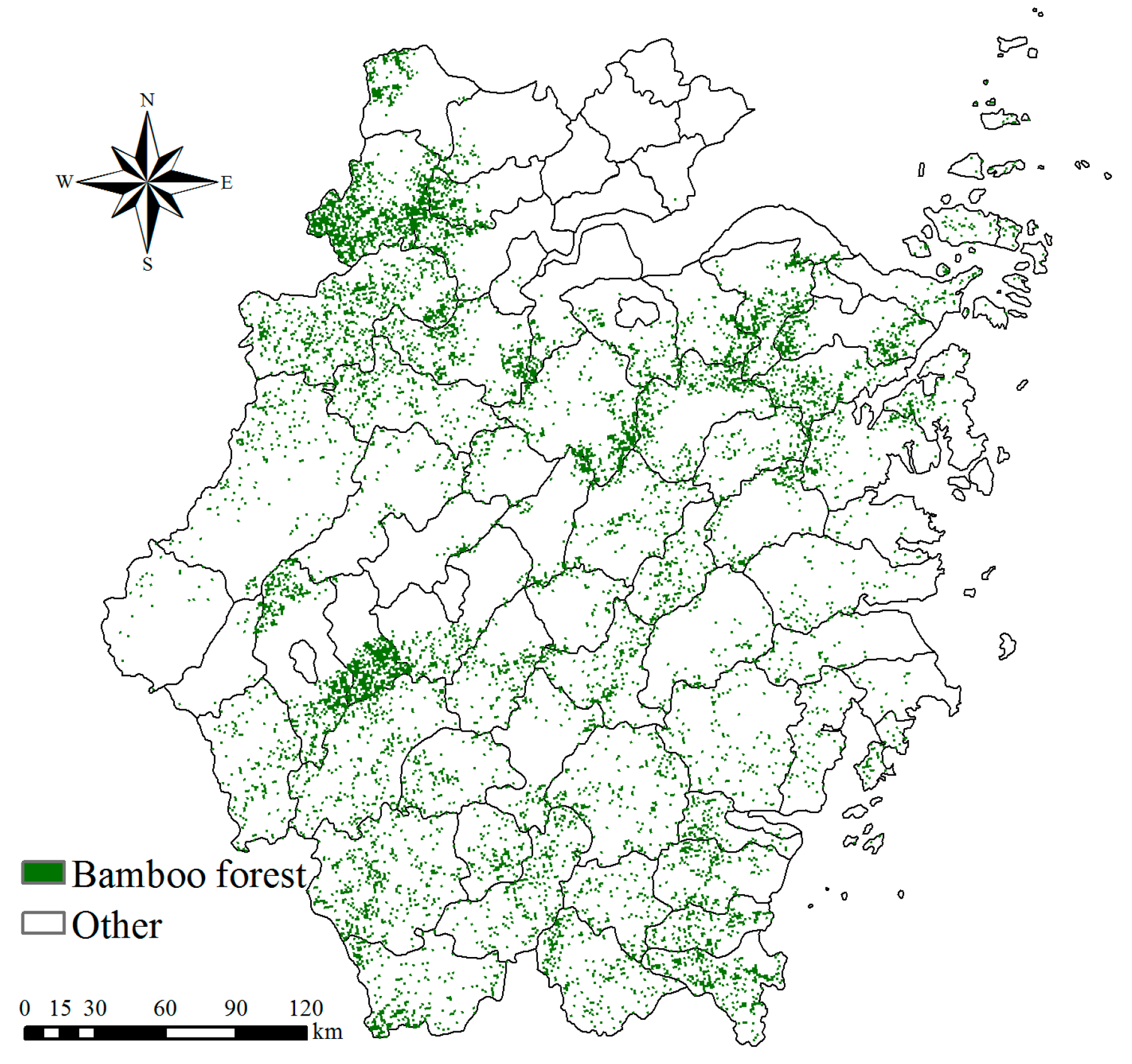
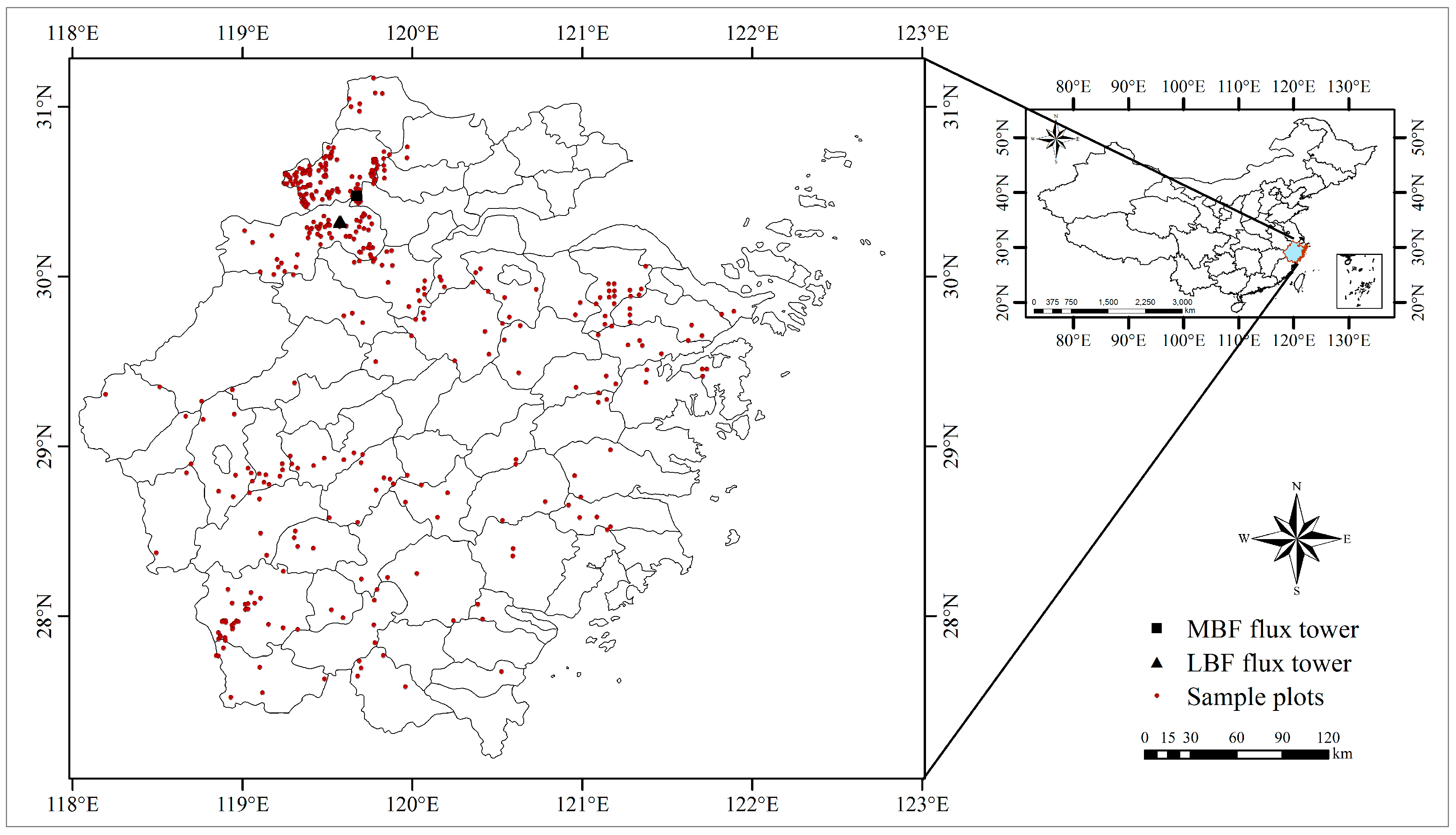
2.1. Study Area

Zhejiang Province is located on the southeast coast of China (27.10°–31.18°N, 118.02°–123.17°E) (Figure 1). This area belongs to a subtropical monsoon zone and enjoys a temperate climate, with well-marked seasons with substantial rainfall and sunshine. By the end of 2014, the province had a total of 6.05 million hectares of forest land, a stumpage of 0.28 billion cubic metres, and a forest coverage rate of 60.91% [34]. Additionally, the bamboo forest area in Zhejiang Province was 0.9 million hectares, which accounted for 14.89% of the total forest area in the province [34].

The MBF flux measurement site is located in Anji County, northwest of Zhejiang Province (30.46°N, 119.66°E). This area has a subtropical monsoon climate with distinct seasons and abundant rainfall; the average January temperature is 2.5 °C, the average July temperature is 27.8 °C, and the average annual precipitation is 1400 mm. The MBF is widely distributed across Anji County, covering an area of 335,484 ha, which accounts for approximately 45% of the total forested area. The area (1 km × 1 km) around the flux tower consists of the MBF. The average diameter of the bamboo at breast height is 9.3 cm, and the canopy height is 12–18 m, with a sparse understory of shrubs and herbs. The Moso bamboo shoots begin to break out from the soil in early March, and the high-growth stage is completed after two to three months [35]. The leaf expansion period of new bamboo starts during the late high-growth stage and is completed within 30 to 40 days [36]. New Moso bamboo changes its leaves in the second year and then every two years after the first leaf changing period [37].

The LBF measurement site is located in the town of Taihuyuan, Lin’an (30.30°N, 119.58°E), which is a well-known “Hometown of Bamboo” in China. Lin’an has a warm and moist subtropical monsoon climate; the annual average temperature is 16 °C, and the average annual precipitation is 1700 mm. The bamboo forest area is 39,052 ha, of which LBF accounts for 19,020 ha. The LBF around the flux tower is typically two to three years old, and it has an average height of 4.5 m, with few shrubs distributed in the understory. Lei bamboo shoots start breaking out from the soil in mid-late February, and they have completed the high-growth stage after approximately 53 days. The leaves of new Lei bamboo start to expand during the late high-growth stage, completing in 15–21 days. Leaf changing occurs every year in the LBF, typically in May and July.

2.2. Datasets and Processing

2.2.1. Satellite Data

The MOD15A2 and MOD09A1 for Zhejiang Province during 2014–2015 were downloaded from NASA’s website (https://ladsweb.nascom.nasa.gov). The original data were reprojected to the WGS84 coordinate system and resampled to 1 km based on the nearest neighbour method using the MODIS Reprojection Tool v4.1. The locally adjusted cubic-spline capping (LACC) method was applied to remove noise in MODIS LAI time-series data [38,39]. The LAI time series of the two flux sites were extracted using the ENVI v5.1. The first (RED) and second (NIR) band of the MOD09A1 dataset were used as observations to optimize the parameters for the canopy reflectance simulation using the PROSAIL model and were used as inputs for LAI assimilation.

Landsat 8 OLI images used for extracting the bamboo forest distribution in Zhejiang Province from June to November in 2014 were downloaded from the United States Geological Survey website (https://earthexplorer.usgs.gov). Details about the selected Landsat images are shown in

Table 1. Details of the Landsat 8 OLI images.

Worldwide Reference System Path/Row	Date	Solar Azimuth Angle (°)	Solar Elevation Angle (°)	Cloud Cover (%)
118/39	13 June 2014	104.06	69.06	10.03
118/40	13 June 2014	100.12	69.12	6.05
118/41	13 June 2014	96.19	69.09	7.94
119/39	22 July 2014	109.15	66.46	2.31
119/40	22 July 2014	105.69	66.66	3.09
119/41	22 July 2014	102.21	66.78	4.02
120/39	11 June 2014	104.49	69.09	1.03
120/40	11 June 2014	100.55	69.17	0.09

. The Landsat images were spatially calibrated, mosaicked, and rectified to the WGS-84 coordinate system. The rectified images were subject to further atmospheric correction using the Fast line-of-sight atmospheric analysis of the hypercubes algorithm [40] and were terrain corrected using ASTER GDEM [41].

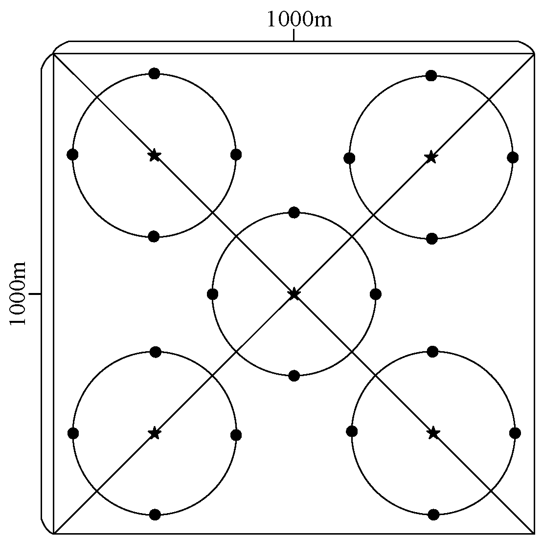
2.2.2. Measurement of LAI

Ground LAI data were collected at the two flux sites for each month. The LAI time series of the MBF extended from spring 2014 to the end of 2015, while that of the LBF extended from winter 2014 to the end of 2015. The LAI was calculated using the LAI (2000G)-LogCI algorithm in the WinSCANOPY v2009a (Regent Instruments Inc., Québec, QC, Canada), based on the canopy images taken in the field using a digital camera with a fish-eye lens. Taking the flux tower as the centre, five observation centres (star in Figure 2) were set across an area of 1 km × 1 km. The LAI of each observation centre was calculated by averaging the LAI observations at the observation centre and in four directions (east, south, west, and north) (black point in Figure 2). Finally, the average value of the five observation centres was calculated as the actual LAI. The plot design of the LAI measurements is shown in Figure 2.

2.2.3. Measurement of Bidirectional Reflectance

The leaf bidirectional reflectance (LBR) and canopy bidirectional reflectance (CBR) were measured using a FieldSpec Pro spectroradiometer (Analytical Spectral Devices Inc., Boulder, CO, USA). This spectroradiometer has a spectral range of 350 nm to 2500 nm, with a resolution of 3 nm (350–1000 nm) and 10 nm (1000 nm–2500 nm), and a sampling interval of 1.4 nm (350–1000 nm) and 2 nm (1000–2500 nm) [42].

The LBR was measured directly using the leaf clip of the analytical spectral device at a sample culm next to each of the flux towers. The detailed measurement process was as follows: First, healthy bamboo around the flux tower was selected, and the canopy of the bamboo was averagely divided into three layers (upper, middle, and lower) [43,44,45]. Second, the spectra of three healthy growth sunlit leaves in each layer were measured, and each leaf was measured 10 times. The average value of 90 measurements was calculated as the LBR [44]. The measurement of each leaf was accomplished within one minute, and the white reference measurement and instrument setting optimization were applied prior to the leaf spectrum measurement. The measured LBR was used when optimizing the parameters of the PROSPECT model (leaf scale).

The CBR was measured using a pistol grip of an analytical spectral device with a field of view of 45° at a height of 1.5 m above the top of the canopy. A total of 40 measurements in four directions (east, south, west, and north) were averaged as the final CBR. The measured CBR was used when optimizing the parameters of the SAIL model (canopy scale).

2.2.4. Measurement of Leaf Biochemical Parameters

The measured leaves were transported to the laboratory inside a temperature-controlled box. The chlorophyll content (C_ab, μg cm⁻²) of the leaves was measured using a spectrophotometer (UV-2102C/PC/PCS, Unico (Shanghai) Instrument Co. Ltd., Shanghai, China) [46]. The leaf area metre was measured using an AM300 (ADC Bioscientific Ltd., Hertfordshire, UK). The fresh weight and dry matter (drying for 48 h at 75 °C) were measured using an FA2104 (Shanghai Liangping Instrument Co. Ltd., Shanghai, China). The difference between the fresh weight and dry matter was calculated as the water content. The dry matter per unit of each leaf was calculated using the dry matter divided by the corresponding leaf area metre, and the water content per unit was calculated in the same way. The average dry matter (C_m, g cm⁻²) and water content (C_w, g cm⁻²) per unit of leaves were used as the inputs of the PROSAIL model.

2.3. Bamboo Forest Distribution Extracting

The bamboo forest distribution was extracted from pre-processed Landsat 8 OLI data using the maximum likelihood method. The training samples included data from 234 fixed plots from the Forest Resources Inventory in Zhejiang Province and 157 investigation plots, as shown in Figure 1. The bamboo forest information was extracted and resampled into pixel sizes of 1 km × 1 km for matching the resolution of MOD09A1 datasets. See [47] for land cover information extracted using Landsat data and the scale transformation method. The extracted bamboo forest map is shown in Figure 3. The map provided accurate locations of the bamboo forest for assimilating the LAI of the bamboo forest in Zhejiang Province.

2.4. LAI Assimilation Method

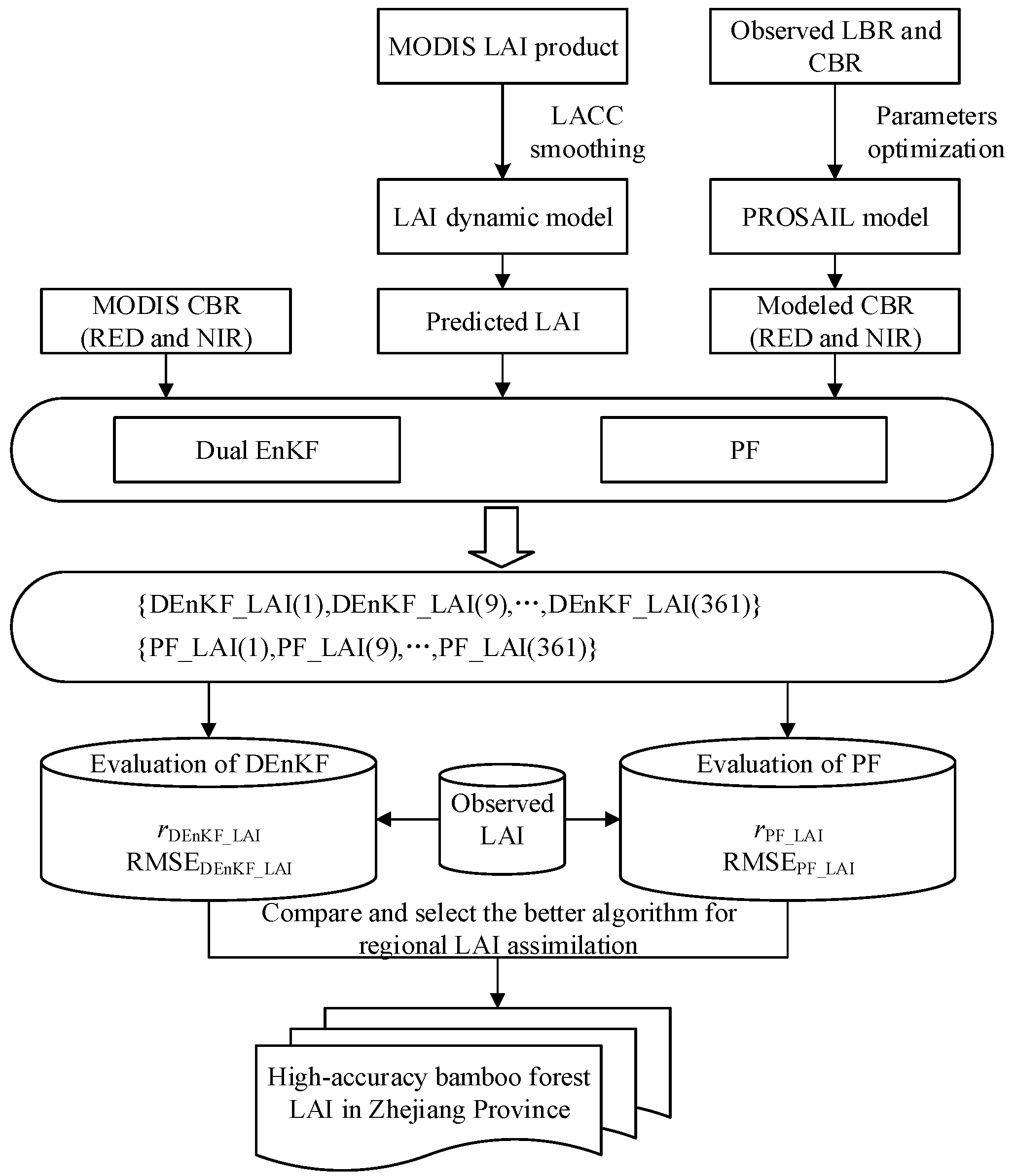
2.4.1. Flow chart of LAI assimilation

The flow chart of the data assimilation and accuracy evaluation of the two data methods is shown in Figure 4. First, the PROSAIL model was optimized using observed LBR and CBR, and was used to simulate the CBR of the MBF and the LBF. Second, the Dual EnKF and PF algorithm was driven by the modelled CBR, MODIS CBR, and LAI simulated by the dynamic model. Third, the performances of the two data assimilation methods were compared using the r and RMSE. Finally, the data assimilation method with the highest r and lowest RMSE was used to generate the high-accuracy LAI products of bamboo forests in Zhejiang Province. The LAI dynamic model, PROSAIL model, Dual EnKF algorithm, and PF algorithm are described in detail in the following sections.

2.4.2. LAI dynamic Model

In this study, the dynamic model is a modified version of the dynamic Leaf Model developed by Dickinson et al. [48]. The model is given by a semi-empirical mathematical formula written as:

$$\frac{dL}{dt}={\lambda }_o\cdot R(x)\cdot L_o\cdot (1-\exp (-c\cdot LA{I}_t))$$

(1)

$$LA{I}_{t+1}=LA{I}_t+{\displaystyle {\int }_t^{t+1}\frac{dL}{dt}}dt-L_t\cdot LA{I}_t+\epsilon$$

(2)

where LAI_t+1 represents the LAI at the previous time step; LAI_t represents the LAI at the current time step; R(x) is a smoothing function; x is the normalization of the LAI; x = (LAI_t − LAI_min)/(LAI_max + LAI_min); LAI_max and LAI_min are the maximum and minimum of the LAI in a year, respectively; L₀ represents the max LAI; L_t represents the rate of leaf litter, which is associated with the biomass of the cluster and plant phenological phases [49]; and λ₀, L₀, L_t, and c are parameters determined based on experience. In this study, the c parameter value is 0.5, and the initial values of the other parameters are obtained according to the field LAI fitting. ε represents the white-noise term with a zero mean and covariance matrix Q, which summarizes all the uncertainties caused by the model formulation, the forcing data, and the model parameters. The initial LAI value of the dynamic model was obtained using the “LAI-CBR” lookup table (see Section 2.4.3).

2.4.3. Simulation of CBR

In this study, PROSAIL, which is a combination of PROSPECT5 and 4SAIL [33], was used to simulate the CBR spectra of the bamboo forest. PROSAIL simulates the top of the CBR in the range of 400 nm to 2500 nm as a function of: (1) canopy structural parameters, i.e., the LAI (m² m⁻²), leaf mesophyll structure parameter (N, unitless), average leaf angle (ALA, °), and hot-spot parameter (H, unitless); (2) biochemical parameters, i.e., C_m, C_w, C_ab, and carotenoids content (C_ar, μg cm⁻²); and (3) viewing geometry parameters, i.e., view zenith angle (θ_v, °), solar zenith angle (θ_s, °), and relative azimuth angle (θ_z, °).

The principal parameters of the PROSAIL model are shown in

Table 2. Principal parameters of the PROSAIL model.

Model	Parameter (Unit)	MBF	LBF	EBDF
PROSPECT5	N	1.04	2.10	2.15
	Cab (μg cm−2)	28–55	30–54	33–65
	Car (μg cm−2)	10	8	10
	Cw (g cm−2)	0.0035	0.0085	0.0150
	Cm (g cm−2)	0.003	0.001	0.009
4SAIL	LAI (m2 m−2)	0.0–7.0	1.5–7.0	0.0–6.5
	ALA (°)	20.2	19.66	19.65
	H	0.0003	0.0015	0.0090
	θv (°)	0–90	0–90	0–90
	θs (°)	0–90	0–90	0–90
	θz (°)	0–180	0–180	0–180

. The observed LAI was used in the optimization of the parameters of the PROSAIL model, whereas the LAI_t was used as the inputs of the PROSAIL model during the assimilation process, as the forest CBR is very sensitive to the LAI [44]. The C_ab varied during the year, according to our measurements. Because C_w and C_m do not vary too significantly during the year, we used the average value of our measurements. θ_v, θ_s, and θ_z varied during the year; refer to the corresponding datasets in the MOD09A1.

Three parameters (N, C_ar, and H) were optimized by comparing the modelled and measured data. First, the parameters of PROSPECT5 were optimized by decreasing the RMSE between the modelled and measured LBR for each forest type. Second, the parameters of 4SAIL for each forest type were optimized using the similarity approach for optimizing the parameters of PROSPECT5. Finally, the optimized PROSAIL model was used to simulate the CBR.

In addition, the PROSAIL model was used to build the “LAI-CBR” lookup table to retrieve the initial LAI value of the dynamic model. The lookup table was generated by various LAI from 0.5 to 7 with a step of 0.1, fixing other parameters and outputting the corresponding CBR. The simulated CBR was resampled to the centre wavelength of MODIS RED and NIR.

2.4.4. Dual EnKF Algorithm

The EnKF algorithm is a sequential data assimilation algorithm based on the Monte Carlo ensemble forecasting method for estimating the forecast error covariance [50]. The greatest advantage of EnKF is that the linear model and the adjoint model do not need to be predicted, which can be used to solve the complex nonlinear Gauss problem [11]. The Dual EnKF has two phases for estimating parameters and state variables: first, the parameters are optimized using the observed state variables; and then, the state variables are updated by optimizing the parameters and observed state variables.

The standard EnKF formula is:

$$A^a=A+K(Y^o-HA)$$

(3)

$$K=P{H}^T{(HP{H}^T+R)}^{-1}$$

(4)

$$P=\frac{1}{N-1}{\displaystyle \sum _{i=1}^N(A-\overline{A}){(A-\overline{A})}^T}$$

(5)

$$P{H}^T=\frac{1}{N-1}{\displaystyle \sum _{i=1}^N(A-\overline{A}){(HA-H\overline{A})}^T}$$

(6)

$$HP{H}^T=\frac{1}{N-1}{\displaystyle \sum _{i=1}^N(HA-H\overline{A}){(HA-H\overline{A})}^T}$$

(7)

where A^a represents the assimilated LAI; A represents the dynamic model forecast LAI; $\overline{A}$ is the ensemble mean of A; Y° represents the perturbed observation ensemble matrix; R and P are the covariance matrices of Y° and A, respectively; H is the observation operator linking the model state and the observation; and T is a matrix transpose. The observation operator H in the standard EnKF is linear, while that in the PROSAIL model is non-linear, which is unsuitable for the standard EnKF. Therefore, an extended ensemble was constructed to transform the nonlinear operator $h(\cdot )$ to a new linear operator $\widehat{H}$. Defining the extended ensemble $\widehat{A}=[\mathrm{A},h(\mathrm{A})]$, Equations (3)–(7) are rewritten as follows:

$$A^a=A+P_e{\widehat{H}}^T{(\widehat{H}{P}_e{\widehat{H}}^T+R)}^{-1}(Y^o-\widehat{H}\widehat{A})$$

(8)

where P_e is the covariance matrix of $\widehat{A}$.

For specific algorithms and procedures related to the Dual EnKF algorithm, please refer to [14].

2.4.5. PF Algorithm

The PF algorithm is a type of Monte Carlo Bayesian algorithm implementation, which is not restricted by the linear model or Gauss’s hypothesis, and is thus applicable to any non-linear and non-Gauss system. Its basic theory is to use a series of weighted particles to approximate the posterior probability density distribution of state variables to better simulate a changing nonlinear system [12]. Assuming that N particles are extracted from the posterior probability distribution of the state variables, the posterior probability density distribution of the state can be obtained by the following equation:

$$\widehat{p}(x_k|z_{1:k})=\frac{1}{N}{\displaystyle \sum _{i=1}^N\delta (x_k-x_k^i)}$$

(9)

where δ is the Dirac function, k represents time, $x_k^i$ represents the particle state value, $z_k$ represents the observation value, and $\widehat{p}(x_k|z_{1:k})$ denotes the posterior probability density distribution. Usually, the posterior distribution density function cannot be obtained directly. To solve this problem, this study used the sequential importance sampling method, which uses a recursive method to calculate the weights of particles using the following equations:

$$w_k^i=w_{k-1}^i\frac{p(z_k|x_k^i)p(x_k^i|x_{k-1}^i)}{q(x_k^i|x_{k-1}^i,z_k)}$$

(10)

$$q(x_k^i|x_{k-1}^i,z_k)=p(x_k^i|x_{k-1}^i)$$

(11)

where $q(x_k^i|x_{k-1}^i,z_k)$ is the importance sampling function, $p(z_k|x_k^i)$ is the likelihood function, and $w_k^i$ represents the weights of the k time particles.

$$w_k^i=w_{k-1}^{i}p(z_k|x_k^i)$$

(12)

Finally, the updated particle weights were obtained according to Equation (14).

$$w_k^i=\frac{w_k^i}{{\displaystyle \sum _{i=1}^N{w}_k^i}}$$

(13)

The estimated value of the state variable is the weighted average of all the state values of the particles.

$${\widehat{x}}_k={\displaystyle \sum _{i=1}^N{w}_k^i{x}_k^i}$$

(14)

For detailed information regarding the PF algorithm and sequential importance sampling method, refer to [16,21]. In this study, the residual resampling method was applied to solve the particle impoverishment problem and ensure the abundance of the particle. For detailed descriptions of the residual resampling method, please refer to [51].

3. Results and Discussion

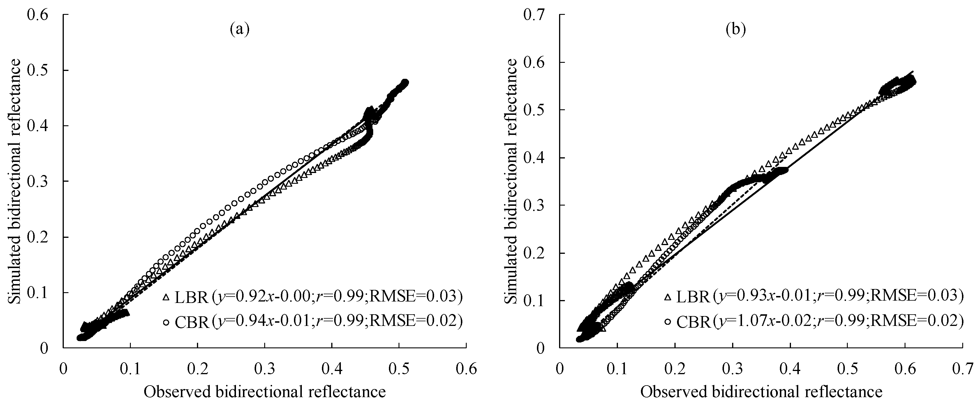
3.1. Validation of Simulated LBR and CBR

The comparisons of observed and simulated bidirectional reflectance by PROSAIL in the MBF and LBF are shown in Figure 5. All the simulated LBR were significantly correlated with the observations, with an r of 0.99. The RMSE of the simulated LBR was 0.02 and 0.03 for the MBF and LBF, respectively, indicating that PROSPECT5 was well calibrated and could be used for CBR simulation. The simulated CBR achieved a high accuracy, with an RMSE of 0.03 and 0.02 for the MBF and LBF, respectively, and provided high-quality inputs for the two LAI assimilation methods.

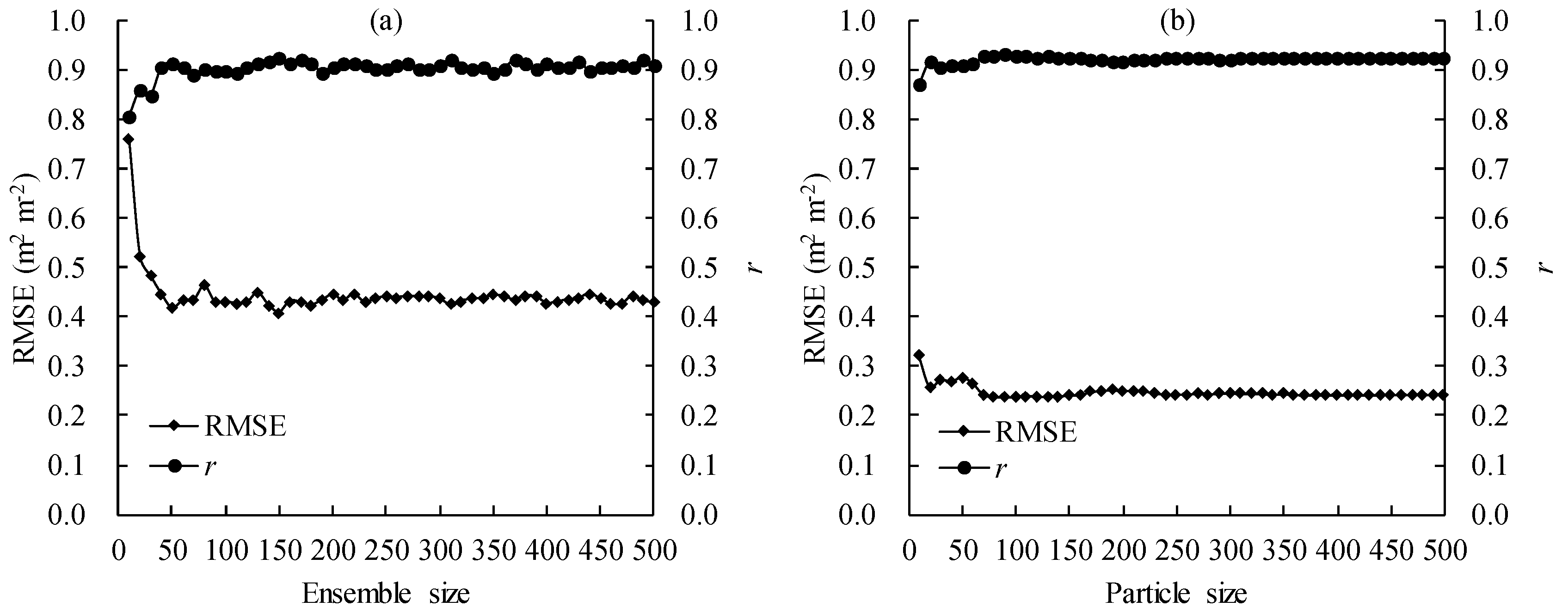
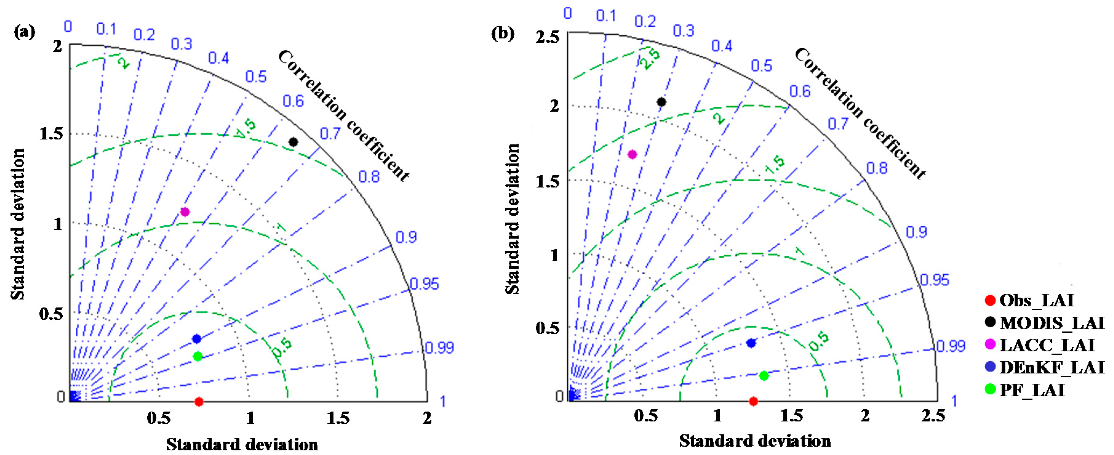
3.2. Performance of Data Assimilation

The performances of the Dual EnKF and PF methods were strongly affected by the size of the ensemble and particles [16,52]. Therefore, the influence of ensemble (particle) size on LAI assimilation was studied. The r and RMSE between the LAI assimilated using different ensemble (particle) sizes and observed during 2015 are shown as Figure 6. The fluctuation of r and RMSE decreased with an increasing ensemble (particle) size, and the r and RMSE stabilized when the ensemble size and particle size were greater than 200 and 80, respectively. The results also indicated that the r increased with an increasing ensemble (particle) size, and the RMSE decreased with an increasing ensemble (particle) size. However, an excessively large ensemble (particle) significantly reduces the computational efficiency [52]. To make the comparison environment of the assimilation results as uniform as possible, this study selected a size of 200 for both the Dual EnKF and PF to assimilate the MODIS LAI.

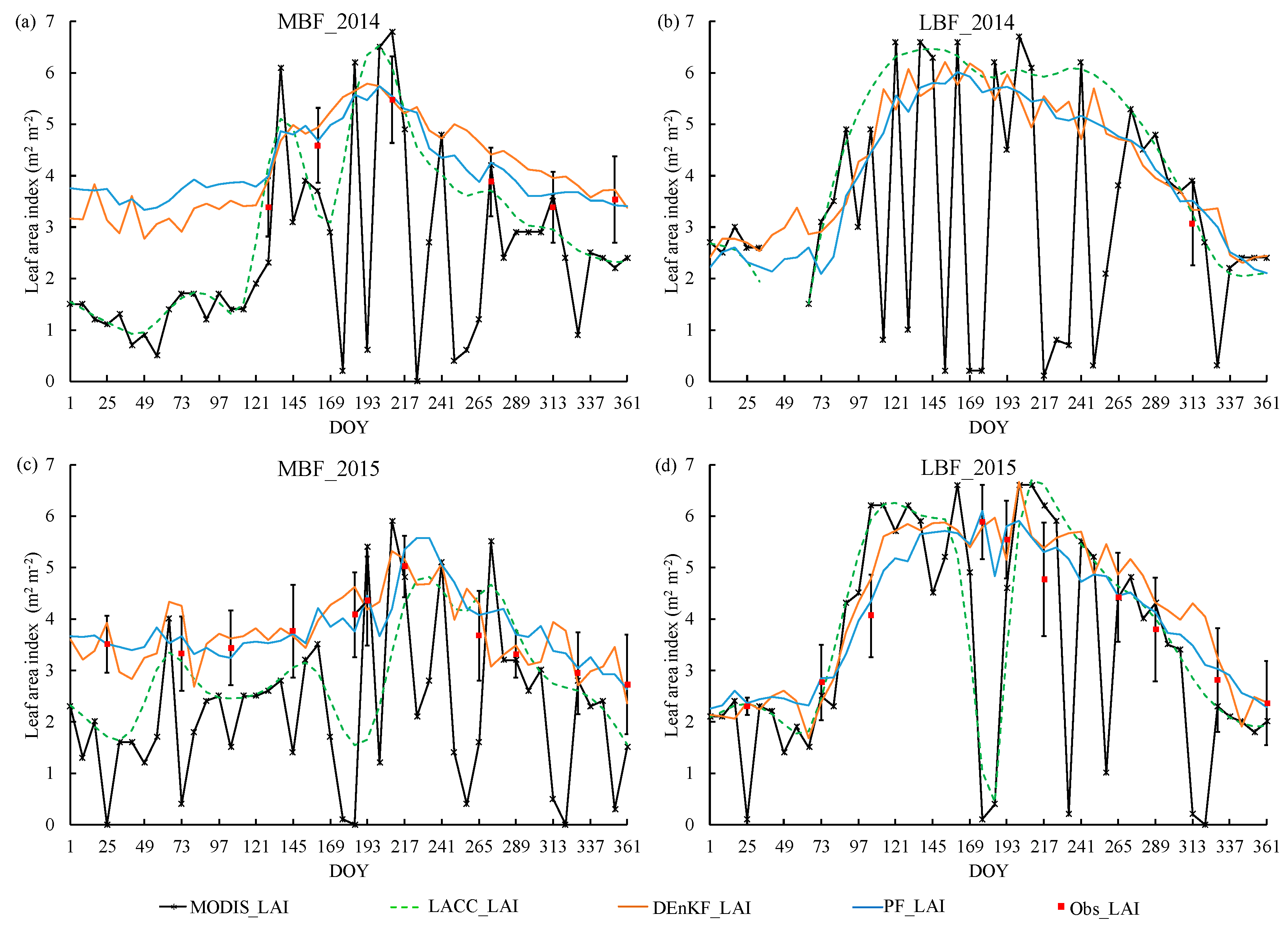
3.3. Validation of LAI Assimilation

The time series of different LAI data are shown in Figure 7, and the Taylor diagram between them is shown in Figure 8. These LAI data include the observed LAI (Obs_LAI), original (MODIS_LAI) and LACC smoothed (LACC_LAI) MODIS LAI products, and the LAI time series assimilated using Dual EnKF (DEnKF_LAI) and PF (PF_LAI) of MBF and LBF during 2014–2015.

As shown in Figure 7, the MODIS_LAI fluctuated considerably in the bamboo forest during 2014–2015, especially during the growing season (e.g., DOY 137–273 in MBF and 89–273 in the LBF in 2014). The lower r and the highest RMSE indicate that there are huge errors in the MODIS LAI time-series data of bamboo forests (Figure 8). The LACC_LAI is smoother than the MODIS_LAI, but still fluctuated during the growing season (e.g., DOY 169–193 in the MBF and LBF in 2015), indicating that the quality of LACC_LAI was significantly affected by the MODIS LAI time series. Moreover, the r between LACC_LAI and Obs_LAI was the lowest, and the RMSE remained very high (Figure 8). Therefore, both the MODIS_LAI and LACC_LAI cannot accurately reflect the long-term LAI variations in bamboo forests.

Compared to MODIS_LAI and LACC_LAI, the DEnKF_LAI and PF_LAI are closer to Obs_LAI, greatly reducing the fluctuations in the MODIS LAI time series, especially during the growing season. Moreover, the two methods increased the r with Obs_LAI and decreased the RMSE, indicating that the assimilated LAI time series greatly decreased the uncertainty in the MODIS LAI time series (Figure 8). However, the errors in DEnKF_LAI were larger than those in PF_LAI, e.g., DEnKF_LAI presents a larger fluctuation with an overestimation during DOY 65–81 in 2015 compared to the PF_LAI. The statistical results also show that PF_LAI was more accurate than DEnKF_LAI: the r of PF_LAI was 4.44% and 4.21% higher than that of DEnKF_LAI for the MBF and LBF, respectively, and the RMSE of PF_LAI was 33.33% lower than that of DEnKF_LAI for both the MBF and LBF (Figure 8).

The reasons for this may be as follows. The EnKF algorithm only provides an optimal estimate of model predictions at the next step of the operation, and it does not consider an optimal estimate of the LAI over annual time periods. Moreover, the EnKF algorithm is a PF with equal weight, whereas the weight was unequal during the assimilation process, which leads to fluctuations in the assimilation process. The PF uses the posterior probability density to calculate the weight of the particles; as such, the assimilated LAI results in a long-term time series that is relatively stable. Therefore, the PF algorithm was more suitable for LAI assimilation for bamboo forests.

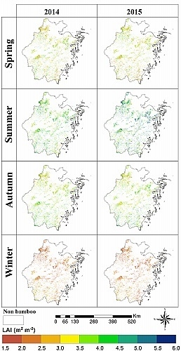
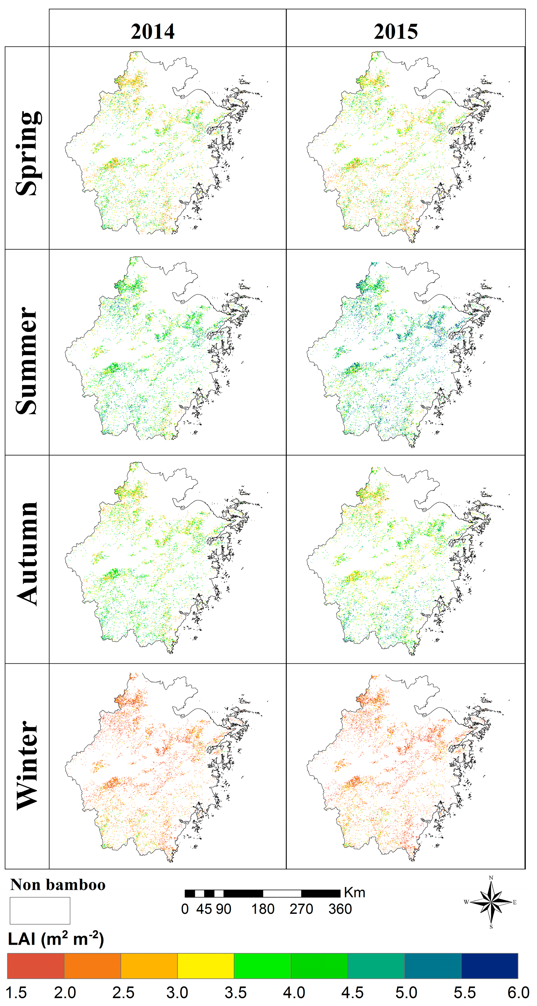
3.4. Assimilating LAI for Bamboo Forests in Zhejiang Province

For the application of large-scale carbon cycle simulations for bamboo forest, the PF algorithm was used to assimilate the MODIS LAI time series in Zhejiang Province. The averaged LAIs of bamboo forest for each season during 2014–2015 are shown in Figure 9, and their statistical information is shown in

Table 3. Statistical information of bamboo forest LAI assimilated by the PF algorithm in Zhejiang Province. Upper-case letters denote significant differences in each row (one-way ANOVA with Duncan’s multiple range test, p < 0.01).

Year	Seasons	LAI (m2 m−2)
		Min	Max	Average ± Std.
2014	Spring	1.81	5.53	3.36 E ± 0.82
	Summer	1.99	5.88	4.04 B ± 0.80
	Autumn	1.94	5.58	3.57 D ± 0.71
	Winter	1.43	4.89	2.23 G ± 0.52
2015	Spring	1.63	5.32	3.21 F ± 0.78
	Summer	2.05	7.48	4.57 A ± 0.93
	Autumn	1.85	6.28	3.68 C ± 0.80
	Winter	1.43	4.44	2.15 H ± 0.50

. The LAI during the summer in 2015 was higher than that in 2014, while the LAI during other seasons in 2015 was similar to that in 2014.

Overall, the LAI of bamboo forests assimilated by the PF algorithm presents a reasonable spatiotemporal pattern in Zhejiang Province. The LAI ranged from 1.63–5.53 during spring (DOY 65–145), with an average value of 3.36 ± 0.82 in 2014 and 3.21 ± 0.78 in 2015. The LAI was highest during summer (DOY 153–241), ranging from 1.99–7.48, with an average value of 4.04 ± 0.80 in 2014 and 4.57 ± 0.93 in 2015. The LAI during autumn (DOY 249–329) was slightly higher than that during spring and ranged from 1.85–6.28, with an average value of 3.57 ± 0.71 in 2014 and 3.68 ± 0.80 in 2015. The LAI was lowest during winter (DOY 337–361), ranging from 1.43–4.44, with an average value of 2.23 ± 0.52 in 2014 and 2.15 ± 0.50 in 2015.

The areas of MBF and LBF accounted for more than 90% of the total bamboo forest area in Zhejiang Province [34], indicating that the assimilated LAI of bamboo forests in Zhejiang Province provides a level of representativeness. The PF algorithm greatly improved the accuracy of MODIS LAI products, and the assimilated LAI can be used as a reliable structure parameter for large-scale carbon cycle simulations in bamboo forests. However, further plot investigations should be conducted to validate the assimilated LAI of other regions.

4. Conclusions

This study compared the performances of two data assimilation methods (Dual EnKF and PF) in improving the quality of MODIS LAI of the MBF and LBF during 2014–2015 using long-term time-series LAI observation data. The study also applied the method with the highest r and lowest RMSE to generate highly accurate LAI products of bamboo forests in Zhejiang Province. The results show that the two methods significantly reduced fluctuations and decreased the uncertainty in MODIS LAI products. The PF_LAI was more accurate than DEnKF_LAI, with an r value of 0.94 and 0.99, and RMSE of 0.28 and 0.28, for the MBF and the LBF, respectively. The average r of PF_LAI was 4.32% higher than that of DEnKF_LAI, and the average RMSE of PF_LAI was 33.33% lower than that of DEnKF_LAI. Therefore, the PF algorithm was applied to assimilate the LAI for bamboo forests in Zhejiang Province. The LAI of bamboo forests assimilated by the PF algorithm in Zhejiang Province ranged between 1.63–5.53, 1.99–7.48, 1.85–6.28, and 1.43–4.89 during Spring, Summer, Autumn, and Winter, respectively. The advantage of the method proposed in this study was the synchronization of the measured LAI involved in the procedure of assimilation and the combined use of the PROSAIL model and data assimilation methods for the assimilation of MODIS LAI. However, the assimilated LAI was highly related to the MODIS reflectance data, indicating that the accuracy of assimilated LAI is affected if large errors exist in the MODIS reflectance data [53]. In future research, the assimilated LAI will be further validated based on plot investigations and applied in simulations of the carbon cycle for bamboo forests using a process-based model.

References

1. Chen, J.M.; Black, T.A. Defining leaf area index for non-flat leaves. Plant Cell Environ. 1992, 15, 421–429. [Google Scholar] [CrossRef]
2. Jonckheere, I.; Fleck, S.; Nackaerts, K.; Muys, B.; Coppin, P.; Weiss, M.; Baret, F. Review of methods for in situ leaf area index determination: Part I. Theories, sensors and hemispherical photography. Agric. For. Meteorol. 2004, 121, 19–35. [Google Scholar] [CrossRef]
3. Chen, J.M.; Cihlar, J. Retrieving leaf area index of boreal conifer forests using landsat tm images. Remote Sens. Environ. 1996, 55, 153–162. [Google Scholar] [CrossRef]
4. Plummer, S.E. Perspectives on combining ecological process models and remotely sensed data. Ecol. Model. 2000, 129, 169–186. [Google Scholar] [CrossRef]
5. Ma, H.; Song, J.L.; Wang, J.D.; Xiao, Z.; Fu, Z. Improvement of spatially continuous forest lai retrieval by integration of discrete airborne lidar and remote sensing multi-angle optical data. Agric. For. Meteorol. 2014, 189, 60–70. [Google Scholar] [CrossRef]
6. Liu, Z.L.; Chen, J.M.; Jin, G.Z.; Qi, Y.J. Estimating seasonal variations of leaf area index using litterfall collection and optical methods in four mixed evergreen–deciduous forests. Agric. For. Meteorol. 2015, 209, 36–48. [Google Scholar] [CrossRef]
7. Heinsch, F.A.; Zhao, M.S.; Running, S.W.; Kimball, J.S.; Nemani, R.R.; Davis, K.J.; Bolstad, P.V.; Cook, B.D.; Desai, A.R.; Ricciuto, D.M.; et al. Evaluation of remote sensing based terrestrial productivity from modis using regional tower eddy flux network observations. IEEE Trans. Geosci. Remote Sens. 2006, 44, 1908–1925. [Google Scholar] [CrossRef]
8. Yan, M.; Tian, X.; Li, Z.Y.; Chen, E.; Wang, X.F.; Han, Z.T.; Sun, H. Simulation of forest carbon fluxes using model incorporation and data assimilation. Remote Sens. 2016, 8, 567. [Google Scholar] [CrossRef]
9. Jiang, J.Y.; Xiao, Z.Q.; Wang, J.D.; Song, J.L. Sequential method with incremental analysis update to retrieve leaf area index from time series modis reflectance data. Remote Sens. 2014, 6, 9194–9212. [Google Scholar] [CrossRef]
10. Disney, M.; Muller, J.-P.; Kharbouche, S.; Kaminski, T.; Voßbeck, M.; Lewis, P.; Pinty, B. A new global fapar and lai dataset derived from optimal albedo estimates: Comparison with modis products. Remote Sens. 2016, 8, 275. [Google Scholar] [CrossRef]
11. Evensen, G. The ensemble kalman filter: Theoretical formulation and practical implementation. Ocean Dyn. 2003, 53, 343–367. [Google Scholar] [CrossRef]
12. Ma, J.W.; Qin, S.X. Recent advances and development of data assimilation algorithms. Adv. Earth Sci. 2012, 27, 747–757. [Google Scholar]
13. Xiao, Z.Q.; Liang, S.L.; Wang, J.D.; Jiang, B.; Li, X.J. Real-time retrieval of leaf area index from modis time series data. Remote Sens. Environ. 2011, 115, 97–106. [Google Scholar] [CrossRef]
14. Li, X.J.; Xiao, Z.Q.; Wang, J.D.; Qu, Y.; Jin, H.A. Dual ensemble kalman filter assimilation method for estimating time series lai. J. Remote Sens. 2014, 18, 27–44. [Google Scholar]
15. Xiong, X.Z.; Navon, I.M.; Uzunoglu, B. A note on the particle filter with posterior gaussian resampling. Tellus A Dyn. Meteorol. Oceanogr. 2006, 58, 456–460. [Google Scholar] [CrossRef]
16. Jiang, Z.W.; Chen, Z.X.; Chen, J.; Liu, J. Application of crop model data assimilation with a particle filter for estimating regional winter wheat yields. IEEE J. Sel. Top. Appl. Earth Obs. Remote Sens. 2014, 7, 4422–4431. [Google Scholar] [CrossRef]
17. Li, X.; Bai, Y.L. A bayesian filter framework for sequential data assimilation. Adv. Earth Sci. 2010, 25, 515–522. [Google Scholar]
18. Jardak, M.; Navon, I.M.; Zupanski, M. Comparison of sequential data assimilation methods for the kuramoto–sivashinsky equation. Int. J. Numer. Methods Fluid 2010, 62, 374–402. [Google Scholar] [CrossRef]
19. Leeuwen, P.J.V. Particle filtering in geophysical systems. Mon. Weather Rev. 2009, 137, 4089–4114. [Google Scholar] [CrossRef]
20. Montzka, C.; Moradkhani, H.; Weihermüller, L.; Franssen, H.-J.H.; Canty, M.; Vereecken, H. Hydraulic parameter estimation by remotely-sensed top soil moisture observations with the particle filter. J. Hydrol. 2011, 399, 410–421. [Google Scholar] [CrossRef]
21. Bi, H.Y.; Ma, J.W.; Qin, S.X.; Zhang, H.J. Simultaneous estimation of soil moisture and hydraulic parameters using residual resampling particle filter. Sci. Chin. Earth Sci. 2014, 57, 824–838. [Google Scholar] [CrossRef]
22. Li, H.; Chen, Z.X.; Wu, W.B.; Jiang, Z.W. Crop model data assimilation with particle filter for yield prediction using leaf area index of different temporal scales. In Proceedings of the 4th International Conference on Agro-Geoinformatics, Istanbul, Turkey, 20–24 July 2015; TARBIL: Istanbul, Turkey, 2015; pp. 4311–4315. [Google Scholar]
23. Tong, G.F.; Fang, Z.; Xu, X.H. A particle swarm optimized particle filter for nonlinear system state estimation. In Proceedings of the IEEE International Conference on Evolutionary Computation, Vancouver, BC, Canada, 16–21 July 2006; IEEE: Vancouver, BC, Canada, 2006; pp. 438–442. [Google Scholar]
24. Yen, T.M. Comparing aboveground structure and aboveground carbon storage of an age series of moso bamboo forests subjected to different management strategies. J. For. Res. 2015, 20, 1–8. [Google Scholar] [CrossRef]
25. Yen, T.M.; Lee, J.S. Comparing aboveground carbon sequestration between moso bamboo (phyllostachys heterocycla) and china fir (cunninghamia lanceolata) forests based on the allometric model. For. Ecol. Manag. 2011, 261, 995–1002. [Google Scholar] [CrossRef]
26. Food and Agriculture Organization of the United Nations (FAO). Global Forest Resources Asessment 2010: Main Report; Food and Agriculture Organization of the United Nations: Rome, Italy, 2010. [Google Scholar]
27. Yen, T.M. Culm height development, biomass accumulation and carbon storage in an initial growth stage for a fast-growing moso bamboo (phyllostachy pubescens). Bot. Stud. 2016, 57, 1–9. [Google Scholar] [CrossRef]
28. Chen, X.G.; Zhang, X.Q.; Zhang, Y.P.; Booth, T.; He, X.H. Changes of carbon stocks in bamboo stands in china during 100 years. For. Ecol. Manag. 2009, 258, 1489–1496. [Google Scholar] [CrossRef]
29. State Forestry Administration, P.R. China (SFAPRC). Forest Resources in China–The 8th National Forest Inventory; State Forestry Administration, P.R. China: Beijing, China, 2015.
30. Yen, T.M.; Wang, C.T. Assessing carbon storage and carbon sequestration for natural forests, man-made forests, and bamboo forests in taiwan. Int. J. Sustain. Dev. World Ecol. 2013, 20, 455–460. [Google Scholar] [CrossRef]
31. Zhou, G.M.; Shi, Y.J.; Lou, Y.P.; Li, J.L.; Yannick, K.; Chen, J.H.; Ma, G.Q.; He, Y.Y.; Wang, X.M.; Yu, T.F. Methodology for Carbon Accounting and Monitoring of Bamboo Afforestation Projects in China; INBAR: Beijing, China, 2013. [Google Scholar]
32. Li, P.H.; Zhou, G.M.; Du, H.Q.; Lu, D.S.; Mo, L.F.; Xu, X.J.; Shi, Y.J.; Zhou, Y.F. Current and potential carbon stocks in moso bamboo forests in china. J. Environ. Manag. 2015, 156, 89–96. [Google Scholar] [CrossRef] [PubMed]
33. Feret, J.B.; François, C.; Asner, G.P.; Gitelson, A.A.; Martin, R.E.; Bidel, L.P.; Ustin, S.L.; le Maire, G.; Jacquemoud, S. Prospect-4 and 5: Advances in the leaf optical properties model separating photosynthetic pigments. Remote Sens. Environ. 2008, 112, 3030–3043. [Google Scholar] [CrossRef]
34. Department of Forestry of Zhejiang Province (DFZP). Announcement of Value of Forest Resources and Ecological Functions of Zhejiang Province in 2014; Department of Forestry of Zhejiang Province: Zhejiang, China, 2015.
35. Fu, J.H. Chinese moso bamboo: Its importance. Bamboo 2001, 22, 5–7. [Google Scholar]
36. Zhou, G.M. Carbon Storage, Fixation and Distribution in Mao Bamboo (Phyllostachys pubescens) Stands Ecosystem; Zhejiang University: Hangzhou, China, 2006. [Google Scholar]
37. Xiao, F.M.; Fan, S.H.; Wang, S.L.; Xiong, C.Y.; Zhang, C.; Liu, S.P.; Zhang, J. Carbon storage and spatial distribution in phyllostachy pubescens and cunninghamia lanceolata plantation ecosystem. Acta Ecol. Sin. 2007, 27, 2794–2801. [Google Scholar]
38. Chen, J.M.; Deng, F.; Chen, M.Z. Locally adjusted cubic-spline capping for reconstructing seasonal trajectories of a satellite-derived surface parameter. IEEE Trans. Geosci. Remote Sens. 2006, 44, 2230–2238. [Google Scholar] [CrossRef]
39. Liu, Y.B.; Ju, W.M.; Chen, J.M.; Zhu, G.L.; Xing, B.L.; Zhu, J.F.; He, M.Z. Spatial and temporal variations of forest lai in china during 2000–2010. Sci. Bull. 2012, 57, 2846–2856. [Google Scholar] [CrossRef]
40. Fan, W.L.; Du, H.Q.; Zhou, G.M. Effects of atmospheric calibration on remote sensing estimation of moso bamboo forest biomass. Chin. J. Appl. Ecol. 2010, 21, 1–8. [Google Scholar]
41. Dong, D.J.; Zhou, G.M.; Du, H.Q. Effects on topographic correction with 6 correction models on phyllostachys praecox forest aboveground biomass estimation. Sci. Silvae Sin. 2011, 47, 1–8. [Google Scholar]
42. Analytical Spectral Devices, Inc. Fieldspec Pro User’s Guide. Available online: http://www.asdi.com (accessed on 7 January 2017).
43. Sun, S.B.; Du, H.Q.; Li, P.H.; Zhou, G.M.; Xu, X.J.; Gao, G.L.; Li, X.J. Retrieval of leaf net photosynthetic rate of moso bamboo forests using hyperspectral remote sen-sing based on wavelet transform. Chin. J. Appl. Ecol. 2016, 27, 49–58. [Google Scholar]
44. Gu, C.Y.; Du, H.Q.; Zhou, G.M.; Han, N.; Xu, X.J.; Zhao, X.; Sun, X.Y. Retrieval of leaf area index of moso bamboo forest with landsat thematic mapper image based on prosail canopy radiative transfer model. Chin. J. Appl. Ecol. 2013, 24, 2248–2256. [Google Scholar]
45. Li, Y.D.; Du, H.Q.; Zhou, G.M.; Gu, C.Y.; Xu, X.J.; Sun, S.B.; Gao, G.L. Chlorophyll content in phyllostachys violascens related to hyper-spectral vegetation indeces and development of an inversion model. J. Zhejiang A F Univ. 2015, 32, 335–345. [Google Scholar]
46. Lu, G.F.; Du, H.Q.; Zhou, G.M.; Lv, Y.L.; Gu, C.Y.; Shang, Z.Z. Dynamic change of phyllostachys edulis forest canopy parameters and their relationships with photosynthetic active radiation in the bamboo shooting growth phase. J. Zhejiang A F Univ. 2012, 29, 844–850. [Google Scholar]
47. Shang, Z.Z.; Zhou, G.M.; Du, H.Q.; Xu, X.J.; Shi, Y.J.; Lü, Y.L.; Zhou, Y.F.; Gu, C.Y. Moso bamboo forest extraction and aboveground carbon storage estimation based on multi-source remotely sensed images. Int. J. Remote Sens. 2013, 34, 5351–5368. [Google Scholar] [CrossRef]
48. Dickinson, R.E.; Tian, Y.H.; Liu, Q.; Zhou, L.M. Dynamics of leaf area for climate and weather models. J. Geophys. Res. 2008, 113, 1–10. [Google Scholar] [CrossRef]
49. Huang, M.; Ji, J.; Cao, M.; Li, K. Modeling study of vegetation shoot and root biomass in china. Acta Ecol. Sin. 2006, 26, 4156–4163. [Google Scholar]
50. Evensen, G. Sequential data assimilation with a nonlinear quasi-geostrophic model using monte carlo methods to forecast error statistics. J. Geophys. Res. Oceans 1994, 99, 10143–10162. [Google Scholar] [CrossRef]
51. Zhang, H.J.; Qin, S.X.; Ma, J.W.; You, H.J. Using residual resampling and sensitivity analysis to improve particle filter data assimilation accuracy. IEEE Geosci. Remote Sens. Lett. 2013, 10, 1404–1408. [Google Scholar] [CrossRef]
52. Rasmussen, J.; Madsen, H.; Jensen, K.H.; Refsgaard, J.C. Data assimilation in integrated hydrological modeling using ensemble kalman filtering: Evaluating the effect of ensemble size and localization on filter performance. Hydrol. Earth Syst. Sci. Discuss. 2015, 12, 2267–2304. [Google Scholar] [CrossRef]
53. Li, X.J.; Mao, F.J.; Du, H.Q.; Zhou, G.M.; Xu, X.J.; Han, N.; Sun, S.B.; Gao, G.L.; Chen, L. Assimilating leaf area index of three typical types of subtropical forest in china from modis time series data based on the integrated ensemble kalman filter and prosail model. ISPRS J. Photogramm. Remote Sens. 2017, 126, 68–78. [Google Scholar] [CrossRef]
Figure 1. The study area and the sample plots of bamboo forest.
Remotesensing 09 00401 g001
Figure 2. Plot design of LAI measurements.
Remotesensing 09 00401 g002
Figure 3. The bamboo forest distribution map of Zhejiang Province.
Remotesensing 09 00401 g003
Figure 4. The flow chart of LAI assimilation for bamboo forests in Zhejiang Province.
Remotesensing 09 00401 g004
Figure 5. The scatter of observed and simulated bidirectional reflectance in the MBF (a) and LBF (b).
Remotesensing 09 00401 g005
Figure 6. Performance of data assimilation for different ensemble sizes (a) and particle sizes (b).
Remotesensing 09 00401 g006
Figure 7. Time series of Obs_LAI, MODIS_LAI and LACC_LAI, DEnKF_LAI and PF_LAI of MBF in 2014 (a) and 2015 (c), and those of LBF in 2014 (b) and 2015 (d).
Remotesensing 09 00401 g007
Figure 8. Taylor diagram between Obs_LAI and other LAI data (MODIS_LAI, LACC_LAI, DEnKF_LAI, and PF_LAI) in (a) MBF and (b) LBF. The radial distance from the origin (black dotted line) is proportional to the standard deviation of the estimate normalized by the standard deviation of the observations, the azimuthal (blue dotted line) position gives the correlation coefficient, and the radial distance from the reference point (green dotted line) is proportional to the centred RMSE difference between the observed and other LAI time series.
Remotesensing 09 00401 g008
Figure 9. LAI assimilated by the PF algorithm in bamboo forests throughout Zhejiang Province.
Remotesensing 09 00401 g009