
Hyperspectral and Multispectral Retrieval of Suspended Sediment in Shallow Coastal Waters Using Semi-Analytical and Empirical Methods


Abstract
:
1. Introduction
2. Materials and Methods
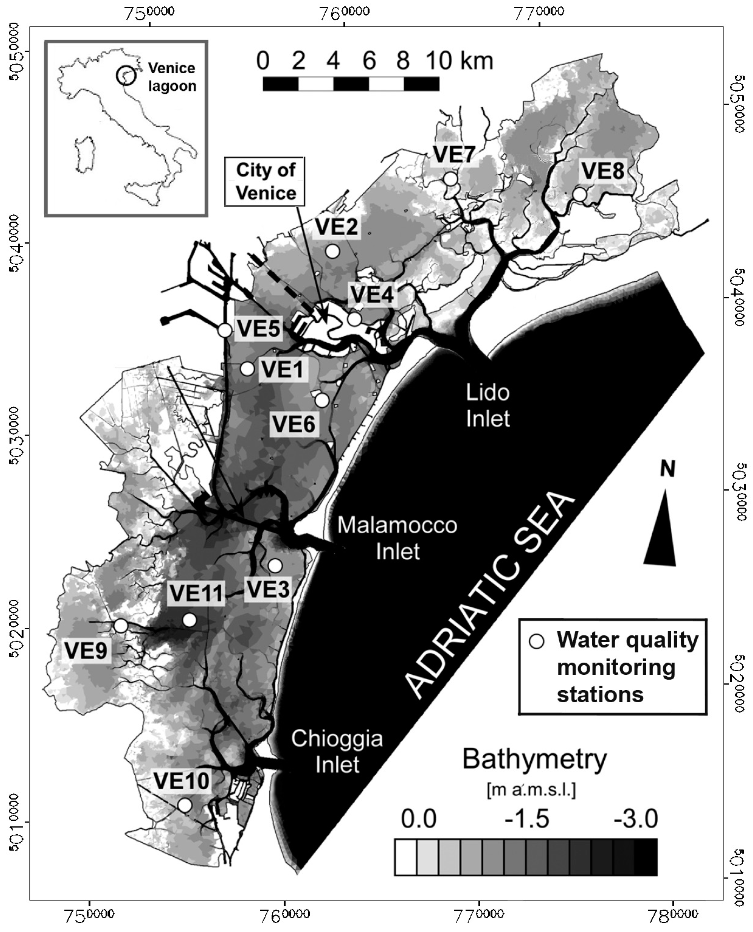
2.1. Study Site and Datasets
2.2. Data Processing
2.3. Radiative Transfer Model
2.4. Empirical Retrieval Models
2.5. Calibration and Validation
2.6. Spectral Band Selection
3. Results
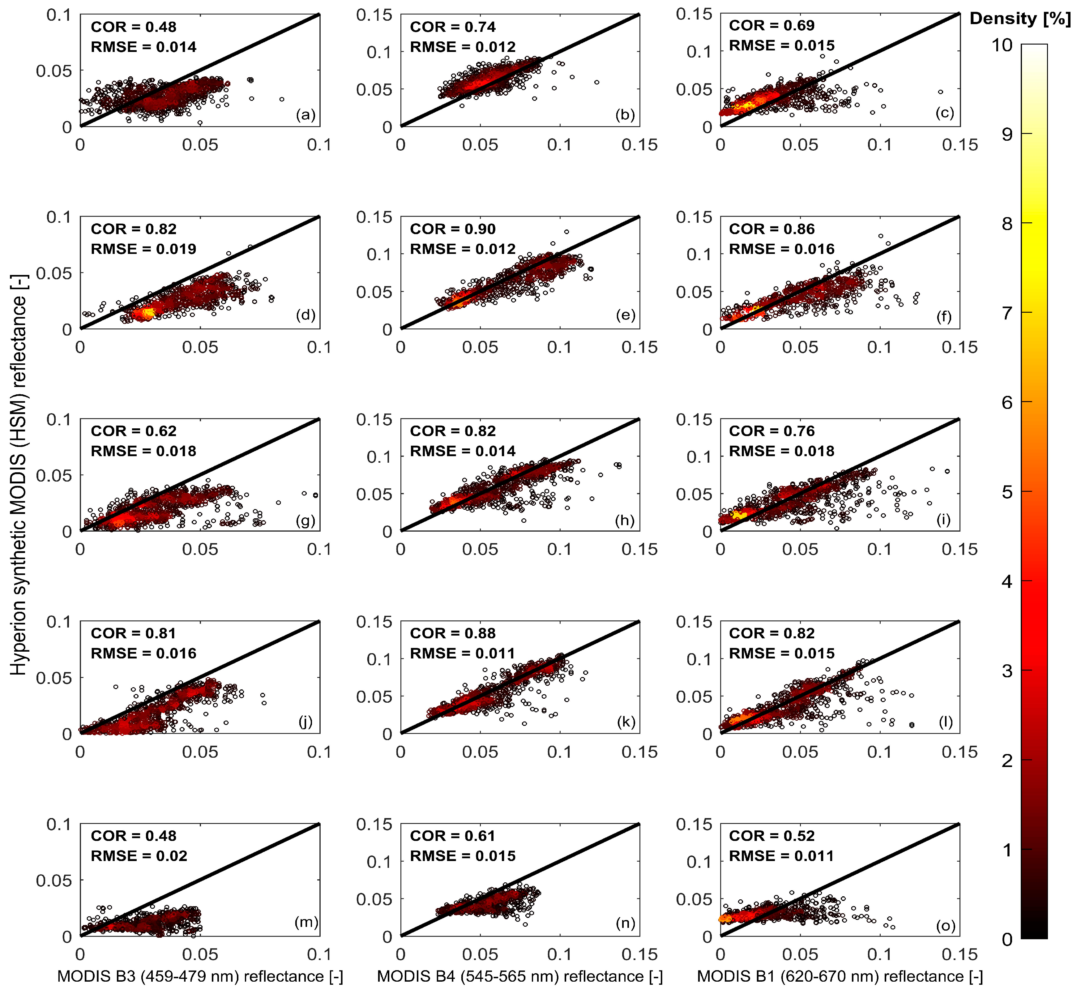
3.1. Atmospheric
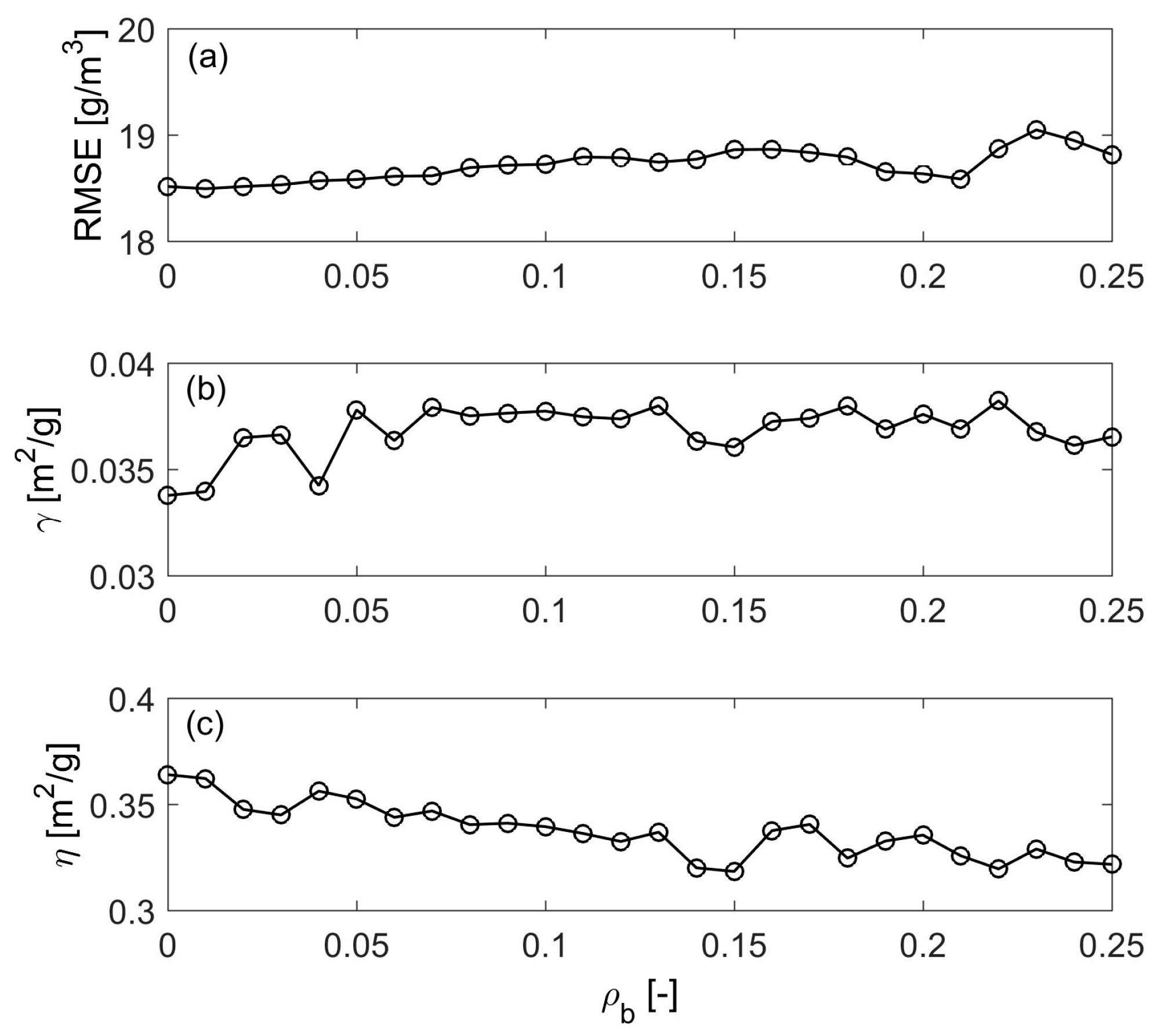
3.2. Evaluation of Bottom Reflectance
3.3. SSC Estimation Using Hyperion Data
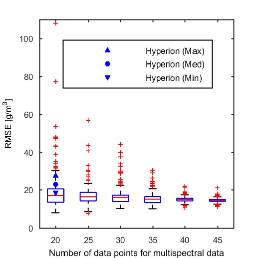
3.4. SSC Estimation Using Multispectral Data
4. Discussion
5. Conclusions
Acknowledgments
Author Contributions
Conflicts of Interest
References
- Carr, J.; D’Odorico, P.; McGlathery, K.; Wiberg, P. Stability and bistability of seagrass ecosystems in shallow coastal lagoons: Role of feedbacks with sediment resuspension and light attenuation. J. Geophys. Res. Biogeosci. 2010, 115, G03011. [Google Scholar] [CrossRef]
- Blum, M.D.; Roberts, H.H. Drowning of the mississippi delta due to insufficient sediment supply and global sea-level rise. Nat. Geosci. 2009, 2, 488–491. [Google Scholar] [CrossRef]
- Carniello, L.; Defina, A.; D’Alpaos, L. Morphological evolution of the venice lagoon: Evidence from the past and trend for the future. J. Geophys. Res. Earth 2009, 114, F04002. [Google Scholar] [CrossRef]
- D’Alpaos, A.; Mudd, S.M.; Carniello, L. Dynamic response of marshes to perturbations in suspended sediment concentrations and rates of relative sea level rise. J. Geophys. Res. Earth 2011, 116, F04020. [Google Scholar] [CrossRef]
- Kirwan, M.L.; Megonigal, J.P. Tidal wetland stability in the face of human impacts and sea-level rise. Nature 2013, 504, 53–60. [Google Scholar] [CrossRef] [PubMed]
- Marani, M.; D’Alpaos, A.; Lanzoni, S.; Carniello, L.; Rinaldo, A. Biologically-controlled multiple equilibria of tidal landforms and the fate of the venice lagoon. Geophys Res. Lett. 2007, 34, L11402. [Google Scholar] [CrossRef]
- Morris, J.T.; Sundareshwar, P.V.; Nietch, C.T.; Kjerfve, B.; Cahoon, D.R. Responses of coastal wetlands to rising sea level. Ecology 2002, 83, 2869–2877. [Google Scholar] [CrossRef]
- Marani, M.; Da Lio, C.; D’Alpaos, A. Vegetation engineers marsh morphology through multiple competing stable states. Proc. Natl. Acad. Sci. USA 2013, 110, 3259–3263. [Google Scholar] [CrossRef] [PubMed]
- Ericson, J.P.; Vorosmarty, C.J.; Dingman, S.L.; Ward, L.G.; Meybeck, M. Effective sea-level rise and deltas: Causes of change and human dimension implications. Glob. Planet. Chang. 2006, 50, 63–82. [Google Scholar] [CrossRef]
- Syvitski, J.P.M.; Kettner, A.J.; Overeem, I.; Hutton, E.W.H.; Hannon, M.T.; Brakenridge, G.R.; Day, J.; Vorosmarty, C.; Saito, Y.; Giosan, L.; et al. Sinking deltas due to human activities. Nat. Geosci. 2009, 2, 681–686. [Google Scholar] [CrossRef]
- Wang, H.J.; Saito, Y.; Zhang, Y.; Bi, N.S.; Sun, X.X.; Yang, Z.S. Recent changes of sediment flux to the western pacific ocean from major rivers in east and southeast asia. Earth-Sci. Rev. 2011, 108, 80–100. [Google Scholar] [CrossRef]
- Yang, S.L.; Milliman, J.D.; Li, P.; Xu, K. 50,000 dams later: Erosion of the yangtze river and its delta. Glob. Planet. Chang. 2011, 75, 14–20. [Google Scholar] [CrossRef]
- Ratliff, K.M.; Braswell, A.E.; Marani, M. Spatial response of coastal marshes to increased atmospheric co2. Proc. Natl. Acad. Sci. USA 2015, 112, 15580–15584. [Google Scholar] [CrossRef] [PubMed]
- Ritchie, J.C.; Zimba, P.V.; Everitt, J.H. Remote sensing techniques to assess water quality. Photogramm. Eng. Remote Sens. 2003, 69, 695–704. [Google Scholar] [CrossRef]
- Petus, C.; Chust, G.; Gohin, F.; Doxaran, D.; Froidefond, J.-M.; Sagarminaga, Y. Estimating turbidity and total suspended matter in the adour river plume (south bay of biscay) using modis 250-m imagery. Cont. Shelf Res. 2010, 30, 379–392. [Google Scholar] [CrossRef]
- Mélin, F.; Zibordi, G.; Berthon, J.-F. Assessment of satellite ocean color products at a coastal site. Remote Sens. Environ. 2007, 110, 192–215. [Google Scholar] [CrossRef]
- Wang, W.; Jiang, W. Study on the seasonal variation of the suspended sediment distribution and transportation in the east china seas based on seawifs data. J. Ocean Univ. China 2008, 7, 385–392. [Google Scholar] [CrossRef]
- Mouw, C.B.; Greb, S.; Aurin, D.; DiGiacomo, P.M.; Lee, Z.; Twardowski, M.; Binding, C.; Hu, C.; Ma, R.; Moore, T. Aquatic color radiometry remote sensing of coastal and inland waters: Challenges and recommendations for future satellite missions. Remote Sens. Environ. 2015, 160, 15–30. [Google Scholar] [CrossRef]
- Matthews, M.W. A current review of empirical procedures of remote sensing in inland and near-coastal transitional waters. Int. J. Remote Sens. 2011, 32, 6855–6899. [Google Scholar] [CrossRef]
- Bissett, W.P.; Arnone, R.A.; Davis, C.O.; Dickey, T.D.; Dye, D.; Kohler, D.D.; Gould, R. From meters to kilometers: A look at ocean-color scales of variability, spatial coherence, and the need for fine-scale remote sensing in coastal ocean optics. Oceanography 2004, 17, 32–43. [Google Scholar] [CrossRef]
- Volpe, V.; Silvestri, S.; Marani, M. Remote sensing retrieval of suspended sediment concentration in shallow waters. Remote Sens. Environ. 2011, 115, 44–54. [Google Scholar] [CrossRef]
- Hellweger, F.; Schlosser, P.; Lall, U.; Weissel, J. Use of satellite imagery for water quality studies in new york harbor. Estuar. Coast. Shelf Sci. 2004, 61, 437–448. [Google Scholar] [CrossRef]
- Baban, S.M. Environmental monitoring of estuaries; estimating and mapping various environmental indicators in breydon water estuary, u. K., using landsat tm imagery. Estuar. Coast. Shelf Sci. 1997, 44, 589–598. [Google Scholar] [CrossRef]
- Carniello, L.; Silvestri, S.; Marani, M.; D’Alpaos, A.; Volpe, V.; Defina, A. Sediment dynamics in shallow tidal basins: In situ observations, satellite retrievals, and numerical modeling in the venice lagoon. J. Geophys. Res. Earth 2014, 119, 802–815. [Google Scholar] [CrossRef]
- Lee, Z.P.; Carder, K.L.; Mobley, C.D.; Steward, R.G.; Patch, J.S. Hyperspectral remote sensing for shallow waters. I. A semianalytical model. Appl. Opt. 1998, 37, 6329–6338. [Google Scholar] [CrossRef] [PubMed]
- Lee, Z.P.; Carder, K.L.; Mobley, C.D.; Steward, R.G.; Patch, J.S. Hyperspectral remote sensing for shallow waters: 2. Deriving bottom depths and water properties by optimization. Appl. Opt. 1999, 38, 3831–3843. [Google Scholar] [CrossRef] [PubMed]
- Santini, F.; Alberotanza, L.; Cavalli, R.M.; Pignatti, S. A two-step optimization procedure for assessing water constituent concentrations by hyperspectral remote sensing techniques: An application to the highly turbid venice lagoon waters. Remote Sens. Environ. 2010, 114, 887–898. [Google Scholar] [CrossRef]
- Brando, V.E.; Dekker, A.G. Satellite hyperspectral remote sensing for estimating estuarine and coastal water quality. IEEE Trans. Geosci. Remote Sens. 2003, 41, 1378–1387. [Google Scholar] [CrossRef]
- Koponen, S.; Attila, J.; Pulliainen, J.; Kallio, K.; Pyhälahti, T.; Lindfors, A.; Rasmus, K.; Hallikainen, M. A case study of airborne and satellite remote sensing of a spring bloom event in the gulf of finland. Cont. Shelf Res. 2007, 27, 228–244. [Google Scholar] [CrossRef]
- Neukermans, G.; Ruddick, K.; Bernard, E.; Ramon, D.; Nechad, B.; Deschamps, P.-Y. Mapping total suspended matter from geostationary satellites: A feasibility study with seviri in the southern north sea. Opt. Express 2009, 17, 14029–14052. [Google Scholar] [CrossRef] [PubMed]
- Odermatt, D.; Gitelson, A.; Brando, V.E.; Schaepman, M. Review of constituent retrieval in optically deep and complex waters from satellite imagery. Remote Sens. Environ. 2012, 118, 116–126. [Google Scholar] [CrossRef]
- Long, C.M.; Pavelsky, T.M. Remote sensing of suspended sediment concentration and hydrologic connectivity in a complex wetland environment. Remote Sens. Environ. 2013, 129, 197–209. [Google Scholar] [CrossRef]
- Binding, C.; Jerome, J.; Bukata, R.; Booty, W. Suspended particulate matter in lake erie derived from modis aquatic colour imagery. Int. J. Remote Sens. 2010, 31, 5239–5255. [Google Scholar] [CrossRef]
- Pearlman, J.S.; Barry, P.S.; Segal, C.C.; Shepanski, J.; Beiso, D.; Carman, S.L. Hyperion, a space-based imaging spectrometer. IEEE Trans. Geosci. Remote Sens. 2003, 41, 1160–1173. [Google Scholar] [CrossRef]
- Seapoint Turbidity Meter: User Manual. Available online: http://www.seapoint.com/pdf/stm_um.pdf (accessed on 18 April 2017).
- Venier, C.; D’Alpaos, A.; Marani, M. Evaluation of sediment properties using wind and turbidity observations in the shallow tidal areas of the venice lagoon. J. Geophys. Res. Earth 2014, 119, 1604–1616. [Google Scholar] [CrossRef]
- Datt, B.; McVicar, T.R.; Van Niel, T.G.; Jupp, D.L.B.; Pearlman, J.S. Preprocessing eo-1 hyperion hyperspectral data to support the application of agricultural indexes. IEEE Trans. Geosci. Remote Sens. 2003, 41, 1246–1259. [Google Scholar] [CrossRef]
- Acharya, P.K.; Berk, A.; Bernstein, L.S.; Matthew, M.W.; Adler-Golden, S.M.; Robertson, D.C.; Anderson, G.P.; Chetwynd, J.H.; Kneizys, F.X.; Shettle, E.P. Modtran User’s Manual; Versions 3.7 and 4.0; Air Force Research Laboratory, Space Vehicles Directorate, Hanscom Air Force Base: Hanscom, MA, USA, 1998. [Google Scholar]
- Analytical Imaging and Geophysics LLC, ACORN 4.0 User’s Guide ENVI Plug-in Version. Available online: http://www.aigllc.com/pdf/acorn4_ume.pdf (accessed 19 April 2017).
- Gao, B.C.; Goetz, A.F.H. Column atmospheric water-vapor and vegetation liquid water retrievals from airborne imaging spectrometer data. J. Geophys. Res. Atmos. 1990, 95, 3549–3564. [Google Scholar] [CrossRef]
- Holben, B.N.; Eck, T.F.; Slutsker, I.; Tanre, D.; Buis, J.P.; Setzer, A.; Vermote, E.; Reagan, J.A.; Kaufman, Y.J.; Nakajima, T.; et al. Aeronet—A federated instrument network and data archive for aerosol characterization. Remote Sens. Environ. 1998, 66, 1–16. [Google Scholar] [CrossRef]
- Shi, W.; Wang, M.H. An assessment of the black ocean pixel assumption for modis swir bands. Remote Sens. Environ. 2009, 113, 1587–1597. [Google Scholar] [CrossRef]
- Knaeps, E.; Dogliotti, A.I.; Raymaekers, D.; Ruddick, K.; Sterckx, S. In situ evidence of non-zero reflectance in the olci 1020 nm band for a turbid estuary. Remote Sens. Environ. 2012, 120, 133–144. [Google Scholar] [CrossRef]
- Richter, R.; Schläpfer, D. Atcor-2/3 User Guide. Available online: http://www.rese.ch/pdf/atcor3_manual.pdf (accessed on 19 April 2017).
- Moses, W.J.; Gitelson, A.A.; Berdnikov, S.; Povazhnyy, V. Estimation of chlorophyll-a concentration in case II waters using modis and meris data-successes and challenges. Environ. Res. Lett. 2009, 4, 045005. [Google Scholar] [CrossRef]
- Vermote, E.F.; Kotchenova, S. Atmospheric correction for the monitoring of land surfaces. J. Geophys. Res. Atmos. 2008, 113, D23S90. [Google Scholar] [CrossRef]
- Kotchenova, S.Y.; Vermote, E.F.; Matarrese, R.; Klemm Jr, F.J. Validation of a vector version of the 6s radiative transfer code for atmospheric correction of satellite data. Part i: Path radiance. Appl. Opt. 2006, 45, 6762–6774. [Google Scholar] [CrossRef] [PubMed]
- Doxaran, D.; Froidefond, J.-M.; Castaing, P.; Babin, M. Dynamics of the turbidity maximum zone in a macrotidal estuary (the gironde, france): Observations from field and modis satellite data. Estuar. Coast. Shelf Sci. 2009, 81, 321–332. [Google Scholar] [CrossRef]
- Miller, R.L.; McKee, B.A. Using modis terra 250 m imagery to map concentrations of total suspended matter in coastal waters. Remote Sens. Environ. 2004, 93, 259–266. [Google Scholar] [CrossRef]
- Petzold, T.J. Volume Scattering Functions for Selected Ocean Waters; Scripps Institution of Oceanography: San Diego, CA, USA, 1972. [Google Scholar]
- Binding, C.E.; Bowers, D.G.; Mitchelson-Jacob, E.G. Estimating suspended sediment concentrations from ocean colour measurements in moderately turbid waters; the impact of variable particle scattering properties. Remote Sens. Environ. 2005, 94, 373–383. [Google Scholar] [CrossRef]
- Ulloa, O.; Sathyendranath, S.; Platt, T. Effect of the particle-size distribution on the backscattering ratio in seawater. Appl. Opt. 1994, 33, 7070–7077. [Google Scholar] [CrossRef] [PubMed]
- Bowers, D.; Binding, C. The optical properties of mineral suspended particles: A review and synthesis. Estuar. Coast. Shelf Sci. 2006, 67, 219–230. [Google Scholar] [CrossRef]
- McKee, D.; Chami, M.; Brown, I.; Calzado, V.S.; Doxaran, D.; Cunningham, A. Role of measurement uncertainties in observed variability in the spectral backscattering ratio: A case study in mineral-rich coastal waters. Appl. Opt. 2009, 48, 4663–4675. [Google Scholar] [CrossRef] [PubMed]
- Zhang, M.; Tang, J.; Song, Q.; Dong, Q. Backscattering ratio variation and its implications for studying particle composition: A case study in yellow and east china seas. J. Geophys. Res. Oceans 2010, 115, C12014. [Google Scholar] [CrossRef]
- Bowers, D.; Braithwaite, K.; Nimmo-Smith, W.; Graham, G. The optical efficiency of flocs in shelf seas and estuaries. Estuar. Coast. Shelf Sci. 2011, 91, 341–350. [Google Scholar] [CrossRef]
- Pope, R.M.; Fry, E.S. Absorption spectrum (380-700 nm) of pure water. 2. Integrating cavity measurements. Appl. Opt. 1997, 36, 8710–8723. [Google Scholar] [CrossRef] [PubMed]
- Babin, M.; Stramski, D.; Ferrari, G.M.; Claustre, H.; Bricaud, A.; Obolensky, G.; Hoepffner, N. Variations in the light absorption coefficients of phytoplankton, nonalgal particles, and dissolved organic matter in coastal waters around europe. J. Geophys. Res. Oceans 2003, 108, 3211. [Google Scholar] [CrossRef]
- Ferrari, G.M.; Tassan, S. On the accuracy of determining light-absorption by yellow substance through measurements of induced fluorescence. Limnol. Oceanogr. 1991, 36, 777–786. [Google Scholar] [CrossRef]
- Haltrin, V.I. One-parameter model of seawater optical properties. In Proceedings of the Ocean Optics XIV CD-ROM, Kailua, HI, USA, 10–13 November 1998. [Google Scholar]
- Doxaran, D.; Cherukuru, R.C.N.; Lavender, S.J. Use of reflectance band ratios to estimate suspended and dissolved matter concentrations in estuarine waters. Int. J. Remote Sens. 2005, 26, 1763–1769. [Google Scholar] [CrossRef]
- Doxaran, D.; Froidefond, J.M.; Lavender, S.; Castaing, P. Spectral signature of highly turbid waters—Application with spot data to quantify suspended particulate matter concentrations. Remote Sens. Environ. 2002, 81, 149–161. [Google Scholar] [CrossRef]
- Lathrop, R.G.; Lillesand, T.M. Monitoring water-quality and river plume transport in green bay, lake-michigan with spot-1 imagery. Photogramm. Eng. Remote Sens. 1989, 55, 349–354. [Google Scholar]
- Nechad, B.; Ruddick, K.G.; Park, Y. Calibration and validation of a generic multisensor algorithm for mapping of total suspended matter in turbid waters. Remote Sens. Environ. 2010, 114, 854–866. [Google Scholar] [CrossRef]
- Tyler, A.N.; Svab, E.; Preston, T.; Presing, M.; Kovacs, W.A. Remote sensing of the water quality of shallow lakes: A mixture modelling approach to quantifying phytoplankton in water characterized by high-suspended sediment. Int. J. Remote Sens. 2006, 27, 1521–1537. [Google Scholar] [CrossRef]
- Chen, Z.M.; Hanson, J.D.; Curran, P.J. The form of the relationship between suspended sediment concentration and spectral reflectance—Its implications for the use of daedalus 1268 data. Int. J. Remote Sens. 1991, 12, 215–222. [Google Scholar] [CrossRef]
- Harrington, J.A.; Schiebe, F.R.; Nix, J.F. Remote-sensing of lake chicot, arkansas—Monitoring suspended sediments, turbidity, and secchi depth with landsat mss data. Remote Sens. Environ. 1992, 39, 15–27. [Google Scholar] [CrossRef]
- Wang, F.; Han, L.; Kung, H.T.; van Arsdale, R.B. Applications of landsat-5 tm imagery in assessing and mapping water quality in reelfoot lake, tennessee. Int. J. Remote Sens. 2006, 27, 5269–5283. [Google Scholar] [CrossRef]
- Wang, X.J.; Ma, T. Application of remote sensing techniques in monitoring and assessing the water quality of taihu lake. Bull. Environ. Contam. Toxicol. 2001, 67, 863–870. [Google Scholar] [CrossRef] [PubMed]
- Wilks, D.S. Statistical Methods in the Atmospheric Sciences, 2nd ed.; Academic Press: Amsterdam, The Netherlands; Boston, MA, USA, 2006. [Google Scholar]
- Sterckx, S.; Knaeps, E.; Bollen, M.; Trouw, K.; Houthuys, R. Retrieval of suspended sediment from advanced hyperspectral sensor data in the scheldt estuary at different stages in the tidal cycle. Mar. Geod. 2007, 30, 97–108. [Google Scholar] [CrossRef]
- Babin, M.; Morel, A.; Fournier-Sicre, V.; Fell, F.; Stramski, D. Light scattering properties of marine particles in coastal and open ocean waters as related to the particle mass concentration. Limnol. Oceanogr. 2003, 48, 843–859. [Google Scholar] [CrossRef]
- Giardino, C.; Brando, V.E.; Dekker, A.G.; Strombeck, N.; Candiani, G. Assessment of water quality in lake garda (Italy) using hyperion. Remote Sens. Environ. 2007, 109, 183–195. [Google Scholar] [CrossRef]
- Bajcsy, P.; Groves, P. Methodology for hyperspectral band selection. Photogramm. Eng. Remote Sens. 2004, 70, 793–802. [Google Scholar] [CrossRef]
- Lee, Z.; Carder, K.L. Effect of spectral band numbers on the retrieval of water column and bottom properties from ocean color data. Appl. Opt. 2002, 41, 2191–2201. [Google Scholar] [CrossRef] [PubMed]
- Lee, Z.; Carder, K.; Arnone, R.; He, M. Determination of primary spectral bands for remote sensing of aquatic environments. Sensors 2007, 7, 3428–3441. [Google Scholar] [CrossRef]
- Kruse, F.A.; Boardman, J.W.; Huntington, J.F. Comparison of airborne hyperspectral data and eo-1 hyperion for mineral mapping. IEEE Trans. Geosci. Remote Sens. 2003, 41, 1388–1400. [Google Scholar] [CrossRef]
- Kruse, F.A.; Boardman, J.W.; Huntington, J.F. Comparison of eo-1 hyperion and airborne hyperspectral remote sensing data for geologic applications. In Proceedings of the IEEE Aerospace Conference, Big Sky, MT, USA, 9–16 March 2002. [Google Scholar]
- Marion, R.; Michel, R.; Faye, C. Atmospheric correction of hyperspectral data over dark surfaces via simulated annealing. IEEE Trans. Geosci. Remote Sens. 2006, 44, 1566–1574. [Google Scholar] [CrossRef]
- Vermote, E.F. Modis Land Reflectance Science Computing Facility. Available online: http://modis-sr.ltdri.org (accessed on 19 April 2017).
- Durand, D.; Bijaoui, J.; Cauneau, F. Optical remote sensing of shallow-water environmental parameters: A feasibility study. Remote Sens. Environ. 2000, 73, 152–161. [Google Scholar] [CrossRef]
- Mobley, C.D. Light and Water: Radiative Transfer in Natural Waters; Academic Press: San Diego, CA, USA, 1994. [Google Scholar]
- Bowers, D.G.; Boudjelas, S.; Harker, G.E.L. The distribution of fine suspended sediments in the surface waters of the irish sea and its relation to tidal stirring. Int. J. Remote Sens. 1998, 19, 2789–2805. [Google Scholar] [CrossRef]
- Hoogenboom, H.J.; Dekker, A.G.; De Haan, J.F. Retrieval of chlorophyll and suspended matter from imaging spectrometry data by matrix inversion. Can. J. Remote Sens. 1998, 24, 144–152. [Google Scholar] [CrossRef]
- Mueller, J.L.; Davis, C.; Arnone, R.; Frouin, R.; Carder, K.; Lee, Z.; Steward, R.; Hooker, S.; Mobley, C.D.; McLean, S. Above-Water Radiance and Remote Sensing Reflectance Measurements and Analysis Protocols; National Aeronautical and Space Administration: Greenbelt, MA, USA, 2000. [Google Scholar]
- Moses, W.J.; Bowles, J.H.; Lucke, R.L.; Corson, M.R. Impact of signal-to-noise ratio in a hyperspectral sensor on the accuracy of biophysical parameter estimation in case ii waters. Opt. Express 2012, 20, 4309–4330. [Google Scholar] [CrossRef] [PubMed]
- Lucke, R.L.; Corson, M.; McGlothlin, N.R.; Butcher, S.D.; Wood, D.L.; Korwan, D.R.; Li, R.R.; Snyder, W.a.; Davis, C.O.; Chen, D.T. Hyperspectral imager for the coastal ocean: Instrument description and first images. Appl. Opt. 2011, 50, 1501–1516. [Google Scholar] [CrossRef] [PubMed]
- Braga, F.; Giardino, C.; Bassani, C.; Matta, E.; Candiani, G.; Strombeck, N.; Adamo, M.; Bresciani, M. Assessing water quality in the northern adriatic sea from hico (tm) data. Remote Sens. Lett. 2013, 4, 1028–1037. [Google Scholar] [CrossRef]
- Shahshahani, B.M.; Landgrebe, D.A. The effect of unlabeled samples in reducing the small sample size problem and mitigating the hughes phenomenon. IEEE Trans. Geosci. Remote Sens. 1994, 32, 1087–1095. [Google Scholar] [CrossRef]
- Landgrebe, D. Information extraction principles and methods for multispectral and hyperspectral image data. Inf. Process. Remote Sens. 1999, 82, 3–38. [Google Scholar]
- Doxaran, D.; Ehn, J.; Bélanger, S.; Matsuoka, A.; Hooker, S.; Babin, M. Optical characterisation of suspended particles in the mackenzie river plume (canadian arctic ocean) and implications for ocean colour remote sensing. Biogeosciences 2012, 9, 3213–3229. [Google Scholar] [CrossRef]
- Hu, C.; Feng, L.; Lee, Z.; Davis, C.O.; Mannino, A.; McClain, C.R.; Franz, B.A. Dynamic range and sensitivity requirements of satellite ocean color sensors: Learning from the past. Appl. Opt. 2012, 51, 6045–6062. [Google Scholar] [CrossRef] [PubMed]
- Carniello, L.; Defina, A.; D’Alpaos, L. Modeling sand-mud transport induced by tidal currents and wind waves in shallow microtidal basins: Application to the venice lagoon (italy). Estuar. Coast. Shelf Sci. 2012, 102, 105–115. [Google Scholar] [CrossRef]
- Dekker, A.G.; Phinn, S.R.; Anstee, J.; Bissett, P.; Brando, V.E.; Casey, B.; Fearns, P.; Hedley, J.; Klonowski, W.; Lee, Z.P. Intercomparison of shallow water bathymetry, hydro-optics, and benthos mapping techniques in australian and caribbean coastal environments. Limnol. Oceanogr. Methods 2011, 9, 396–425. [Google Scholar] [CrossRef]
- Ali, K.; Witter, D.; Ortiz, J. Application of empirical and semi-analytical algorithms to meris data for estimating chlorophyll a in case 2 waters of lake erie. Environ. Earth Sci. 2014, 71, 4209–4220. [Google Scholar] [CrossRef]
- Vermote, E.; Justice, C.; Claverie, M.; Franch, B. Preliminary analysis of the performance of the landsat 8/oli land surface reflectance product. Remote Sens. Environ. 2016, 185, 46–56. [Google Scholar] [CrossRef]
- Härmä, P.; Vepsäläinen, J.; Hannonen, T.; Pyhälahti, T.; Kämäri, J.; Kallio, K.; Eloheimo, K.; Koponen, S. Detection of water quality using simulated satellite data and semi-empirical algorithms in finland. Sci. Total Environ. 2001, 268, 107–121. [Google Scholar] [CrossRef]
- Lee, Z.; Casey, B.; Arnone, R.; Weidemann, A.; Parsons, R.; Montes, M.J.; Gao, B.C.; Goode, W.; Davis, C.O.; Dye, J. Water and bottom properties of a coastal environment derived from hyperion data measured from the eo-1 spacecraft platform. J. Appl. Remote Sens. 2007, 1, 011502. [Google Scholar] [CrossRef]
- Devred, E.; Turpie, K.R.; Moses, W.; Klemas, V.V.; Moisan, T.; Babin, M.; Toro-Farmer, G.; Forget, M.H.; Jo, Y.H. Future retrievals of water column bio-optical properties using the hyperspectral infrared imager (hyspiri). Remote Sens. 2013, 5, 6812–6837. [Google Scholar] [CrossRef]


| Product (Preprocessing Level) | Spectral Band and Range (μm) | Spatial Resolution (m) | Number of Images | Date of Acquisition | Solar Azimuth (Degree) | Solar Zenith (Degree) | Satellite Zenith (Degree) | Aerosol Optical Thickness at 550 nm 1 |
|---|---|---|---|---|---|---|---|---|
| Hyperion (1R) | B12–B35: 0.467–0.701 B141–B160: 1.56–1.75 | 30 | 5 | 10 Februar2005 | 153.8 | 63.4 | 3.2 | 0.21 |
| 18 June 2005 | 135.2 | 27.6 | 3.0 | 0.40 | ||||
| 4 July 2005 | 135.5 | 28.5 | 3.1 | 0.40 | ||||
| 20 July 2005 | 136.1 | 30.6 | 3.3 | 0.34 | ||||
| 7 Januar 2006 | 157.7 | 70.8 | −0.3 | 0.23 | ||||
| Landsat TM (1R) | B3: 0.63–0.69 | 30 | 2 | 8 December 2001 | 159.1 | 71.5 | Nadir | 0.05 |
| 25 June 2007 | 134.2 | 27.3 | 0.24 | |||||
| Landsat ETM+ (1R) | B3: 0.63–0.69 | 30 | 2 | 14 September 2002 | 151.2 | 46.2 | Nadir | 0.35 |
| 11 December 2005 | 161.2 | 71.3 | 0.10 | |||||
| ASTER (1B) | B2: 0.63–0.69 | 15 | 8 | 26 May 2005 | 148.8 | 27.1 | Nadir | 0.11 |
| 11 June 2005 | 145.6 | 25.6 | 0.31 | |||||
| 13 July 2005 | 144.7 | 27.3 | 0.20 | |||||
| 29 July 2005 | 146.7 | 30.4 | 0.37 | |||||
| 14 June 2006 | 145.3 | 25.5 | 0.17 | |||||
| 24 June 2007 | 148.5 | 25.1 | 0.14 | |||||
| 10 July 2007 | 147.8 | 26.1 | 0.04 | |||||
| 5 September 2007 | 157.4 | 40.6 | 0.02 | |||||
| ALOS (1B1) | B3: 0.61–0.69 | 10 | 1 | 8 July 2007 | 145.9 | 26.1 | Nadir | 0.08 |
| Name | Description (Unit) | Value (Range) | Source |
|---|---|---|---|
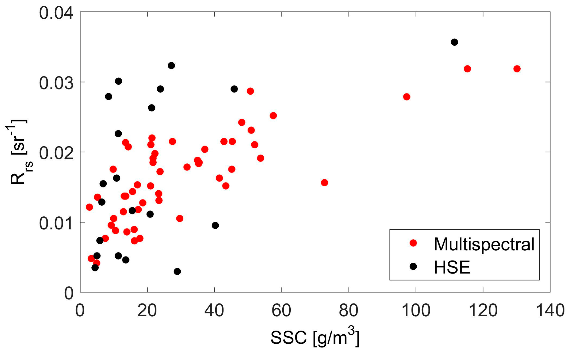
| Rrs(λ) | Above surface remote sensing reflectance (460 to 700 nm) (sr−1) | 0.01–0.04 | 1 |
| Bottom reflectance (460 to 700 nm) | 0.05–0.09 | 2 | |
| H | Water depth (m) | 1.2–2.5 | 3 |
| Subsurface solar zenith angle (rad) | 0.35–0.78 | 1 | |
| Absorption coefficient of pure water (460 to 700 nm) (m−1) | 0.01–0.64 | 4 | |
| Phytoplankton-specific absorption coefficient (460 to 700 nm) (m2/mg) | 0.001–0.027 | 5 | |
| Colored dissolved organic matter (CDOM)-specific absorption coefficient at 375 nm (m−1) | 1.25 | 2 | |
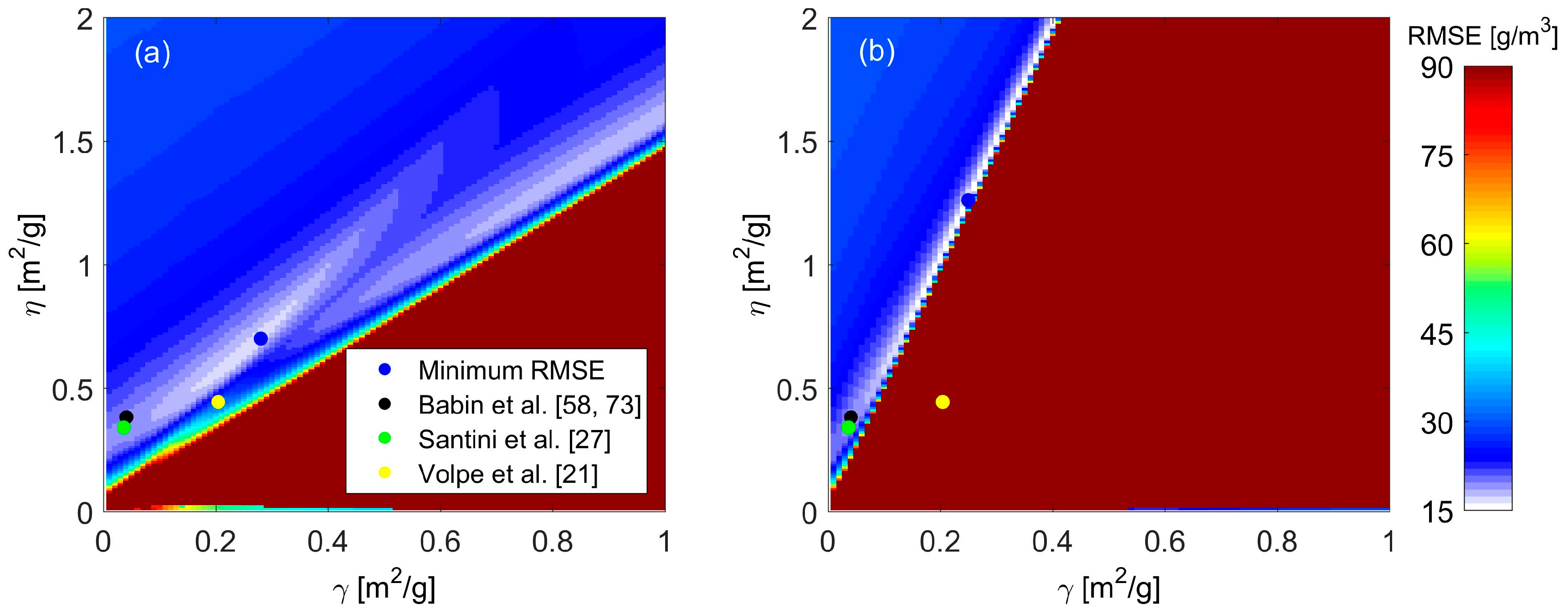
| Suspended sediment specific backscattering coefficient at 400 nm (m2/g) | 0.34, 0.38 | 5, 6 | |
| Suspended sediment specific absorption coefficient at 443 nm (m2/g) | 0.033–0.067 | 7 | |
| CC | Chlorophyll-a concentration (mg/m3) | 0.2–6.8 | 3 |
| SSC | Suspended sediment concentration (g/m3) | 4–100 | 3 |
| Calibration RMSE (g/m3) | Validation RMSE (g/m3) | Difference between Calibration and Validation (g/m3) | |
|---|---|---|---|
| Spectral bands from 460 nm to 700 nm | 17.56 | 27.00 | 9.44 |
| Spectral bands centered at 660 nm | 15.56 | 22.48 | 6.92 |
| Spectral bands centered at 560 nm | 17.68 | 23.81 | 6.13 |
| Calibration RMSE (g/m3) | Validation RMSE (g/m3) | Difference between Calibration and Validation (g/m3) | |
|---|---|---|---|
| RTM-inversion | 13.57 | 14.12 | 0.55 |
| Linear regression | 18.52 | 19.24 | 0.72 |
| Second-order polynomial regression | 14.94 | 16.05 | 1.11 |
© 2017 by the authors. Licensee MDPI, Basel, Switzerland. This article is an open access article distributed under the terms and conditions of the Creative Commons Attribution (CC BY) license (http://creativecommons.org/licenses/by/4.0/).
Share and Cite
Zhou, X.; Marani, M.; Albertson, J.D.; Silvestri, S. Hyperspectral and Multispectral Retrieval of Suspended Sediment in Shallow Coastal Waters Using Semi-Analytical and Empirical Methods. Remote Sens. 2017, 9, 393. https://doi.org/10.3390/rs9040393
Zhou X, Marani M, Albertson JD, Silvestri S. Hyperspectral and Multispectral Retrieval of Suspended Sediment in Shallow Coastal Waters Using Semi-Analytical and Empirical Methods. Remote Sensing. 2017; 9(4):393. https://doi.org/10.3390/rs9040393
Chicago/Turabian StyleZhou, Xiaochi, Marco Marani, John D. Albertson, and Sonia Silvestri. 2017. "Hyperspectral and Multispectral Retrieval of Suspended Sediment in Shallow Coastal Waters Using Semi-Analytical and Empirical Methods" Remote Sensing 9, no. 4: 393. https://doi.org/10.3390/rs9040393