Article

Evapotranspiration Mapping in a Heterogeneous Landscape Using Remote Sensing and Global Weather Datasets: Application to the Mara Basin, East Africa

by
Tadesse Alemayehu
1,*,†,
Ann van Griensven
1,2,
Gabriel B. Senay
3 and
Willy Bauwens
1
1
Department of Hydrology and Hydraulic Engineering, Vrije Universiteit Brussel (VUB), Pleinlaan 2, 1050 Brussels, Belgium
2
Department of Water Science and Engineering, IHE Delft, P.O. Box 3015, 2601 DA Delft, The Netherlands
3
USGS Earth Resource Observation and Science (EROS) Center, North Central Climate Science Center, Colorado State University, Fort Collins, CO 80523-1499, USA
*
Author to whom correspondence should be addressed.
Current address: Department ofWater Science and Engineering, IHE Delft, P.O. Box 3015, 2601 DA Delft, The Netherlands
Remote Sens. 2017, 9(4), 390; https://doi.org/10.3390/rs9040390
Submission received: 19 October 2016 / Revised: 10 April 2017 / Accepted: 17 April 2017 / Published: 20 April 2017

Abstract

:
Actual evapotranspiration (ET) is a major water use flux in a basin water balance with crucial significance for water resources management and planning. Mapping ET with good accuracy has been the subject of ongoing research. Such mapping is even more challenging in heterogeneous and data-scarce regions. The main objective of our research is to estimate ET using daily Moderate Resolution Imaging Spectroradiometer (MODIS) land surface temperature and Global Land Data Assimilation System (GLDAS) weather datasets based on the operational simplified surface energy balance (SSEBop) algorithm at a 1-km spatial scale and 8-day temporal resolution for the Mara Basin (Kenya/Tanzania). Unlike previous studies where the SSEBop algorithm was used, we use a seasonally-varying calibration coefficient for determining the “cold” reference temperature. Our results show that ET is highly variable, with a high inter-quartile range for wetlands and evergreen forest (24% to 29% of the median) and even up to 52% of the median for herbaceous land cover and rainfed agriculture. The basin average ET accounts for about 66% of the rainfall with minimal inter-annual variability. The basin scale validation using nine-years of monthly, gridded global flux tower-based ET (GFET) data reveals that our ET is able to explain 64% of the variance in GFET while the MOD16-NB (Nile Basin) explains 72%. We also observe a percent of bias (PBIAS) of 1.1% and 2.8%, respectively for SSEBop ET and MOD16-NB, indicating a good reliability in the ET estimates. Additionally, the SSEBop ET explains about 52% of the observed variability in the Normalized Difference Vegetation Index (NDVI) for a 16-day temporal resolution and 81% for the annual resolution, pointing to an increased reliability for longer aggregation periods. The annual SSEBop ET estimates are also consistent with the underlying primary (i.e., water and energy) and secondary (i.e., soil, topography, geology, land cover, etc.) controlling factors across the basin. This paper demonstrated how to effectively estimate and evaluate spatially-distributed and temporally-varying ET in data-scarce regions that can be applied elsewhere in the world where observed hydro-meteorological variables are limited.

Graphical Abstract

1. Introduction

Actual evapotranspiration (ET) is a major component in a basin water balance that interlinks the biosphere, the hydrosphere and the atmosphere. Accurate information about ET has practical significance in water resources planning and management, irrigation scheduling, water regulation and environmental issues, among others [1,2]. ET is highly variable both spatially and temporally because of the high variability in vegetation, water availability and climate influences [3].
The classic point and/or field-scale ET measurement techniques include a variety of methods ranging from lysimeters to eddy covariance and scintillometry. The applications of these methods are limited to field scale [4] and do not provide the spatial distribution over large areas/basins. On the other hand, the remote sensing-based surface energy balance (SEB) models provide ET estimates both at field and regional scale [5,6,7] with reasonable accuracy. Recently, Karimi and Bastiaanssen [7] reviewed several published validation results on the reliability of remote sensing algorithms to derive spatially-distributed ET spanning at least one growing season. Their assessment showed that the absolute values of ET can be estimated with an overall accuracy of 95%. Gowda et al. [6] reported accuracies that vary from 67% to 97% for daily ET and rise above 94% for seasonal ET. Generally, the accuracy levels from validation studies indicate that remote sensing-based SEB models are reliable for mapping ET at different spatial and temporal scales. As noted in McCabe et al. [8], the variability in accuracy level and ET estimation skills is mainly ascribed to model structures and parametrization choices and forcing dataset quality. Additionally, Kalma et al. [5] underscored, after reviewing 30 published validation studies, that more complex physical and analytical methods are not necessarily more accurate than empirical and statistical approaches. Data-intensive, but physically-based SEB models, such as the Surface Energy Balance System (SEBS), are more sensitive to the quality of the forcing data than models with fewer inputs [8]. Such findings make the applications of simplified SEB appealing in data-scarce basins. We therefore use the “Operational Simplified Surface Energy Balance model” (SSEBop) [9] for mapping ET in this study. Like the more complex SEB model, remotely-sensed land surface temperature (Ts) is the primary forcing for the SSEBop.
The SSEBop has been applied at the regional scale for different climates and landscapes [9,10,11]. Senay et al. [9] produced ET estimates for the contiguous United States and reported that the SSEBop estimated ET explained 64% of the observed monthly ET across diverse ecosystems. Velpuri et al. [11] also evaluated annual SSEBop ET estimates using ET estimates from eddy covariance and basin water balance at point and basin scales across a range of land cover, elevation and climate zones. Their analyses showed that the SSEBop ET performance variability with coefficient of determination (R2) values varied from 0.57 to 0.81 (across land cover types), from 0.54 to 0.78 (across climatic zones) and from 0.57 to 0.75 (across elevation zones).
Several studies compared the performance of SSEBop against more complex SEB models: Surface Energy Balance Algorithm for Land (SEBAL), Mapping ET at high Resolution with Internalized Calibration (METRIC), SEBS and the Moderate Resolution Imaging Spectroradiometer (MODIS) global ET product (MOD16) [11,12,13]. Velpuri et al. [11] observed a comparable accuracy for SSEBop and MOD16 monthly ET products across the conterminous United States for several land cover types. Their inter-comparison showed good performance of MOD16 for cropland (R2 = 0.70) and woody savanna (R2 = 0.71) classes, while SSEBop showed higher Taylor skill scores (>0.70) for most of the land cover types. In contrast, Bhattarai et al. [12] compared daily ET estimates from five SEB models (SEBAL, SEBS, METRIC, Simplified Surface Energy Balance Index (S-SEBI) and SSEBop) using measured ET at four sites (marsh, grass and citrus surfaces) in the humid southeastern United States. They found that SEBS gave the best results, while SSEBop had the lowest performance. Furthermore, they reported a mean difference of 6 K between the SSEBop cold reference temperature (Tc) and the manually-selected cold pixels for the SEBAL and METRIC models, and the weak performance of SSEBop was mainly attributed to overestimations in the Tc. Partly, this limitation is associated with the constant calibration coefficient used for determining the Tc. Therefore, we propose to use a seasonally-varying calibration coefficient, as also suggested by Senay et al. [14].
The transboundary Mara River Basin (Kenya/Tanzania), characterized by rich biodiversity and diverse agroecosystems, is home to the world-famous Masai-Mara National Reserve and part of the Serengeti National Park; thereby, the limited water resources have profound socio-economic and ecological importance. However, the basin’s spatio-temporal water balance dynamics have not been well investigated, mainly due to poor monitoring of the hydro-meteorological variables. Therefore, remotely-sensed Earth observation products and global reanalysis weather datasets offer the opportunity to map ET at low cost that is essential to better understand the underlying factors that affect the water availability and the water balance. To the best knowledge of the authors, this is the first contribution focusing on ET modeling for the Mara Basin. Thus, our goal is to map ET at a 1-km spatial scale and eight-day temporal resolution using routinely-available daily MODIS Ts and Global Land Data Assimilation System (GLDAS) weather dataset-based modified SSEBop parameterization. Most studies on ET mapping using a global gridded weather dataset and remote sensing products have been at the global and regional scale. The reliability of these dataset for modeling ET at the basin scale has not received much attention, and hence, our paper also contributes towards this. As in situ ET observations are non-existent in the region, the monthly observation-based, globally-gridded flux tower network (FLUXNET) ET (GFET) [15] is used to validate our ET estimates and the regional MOD16 ET product (MOD16-NB (Nile Basin)) at the basin scale. Subsequently, the SSEBop ET and MOD16-NB are inter-compared to explore the extent of their discrepancy and/or agreements at the land cover level. The MODIS NDVI time series is also employed for evaluating the ET estimates per land-cover classes, while Budyko’s principle is used to evaluate the consistency of the SSEBop ET across watersheds. We believe this research will shed light on the major challenges and available alternatives for ET modeling in data-scarce basins elsewhere in the world.

2. Materials and Methods
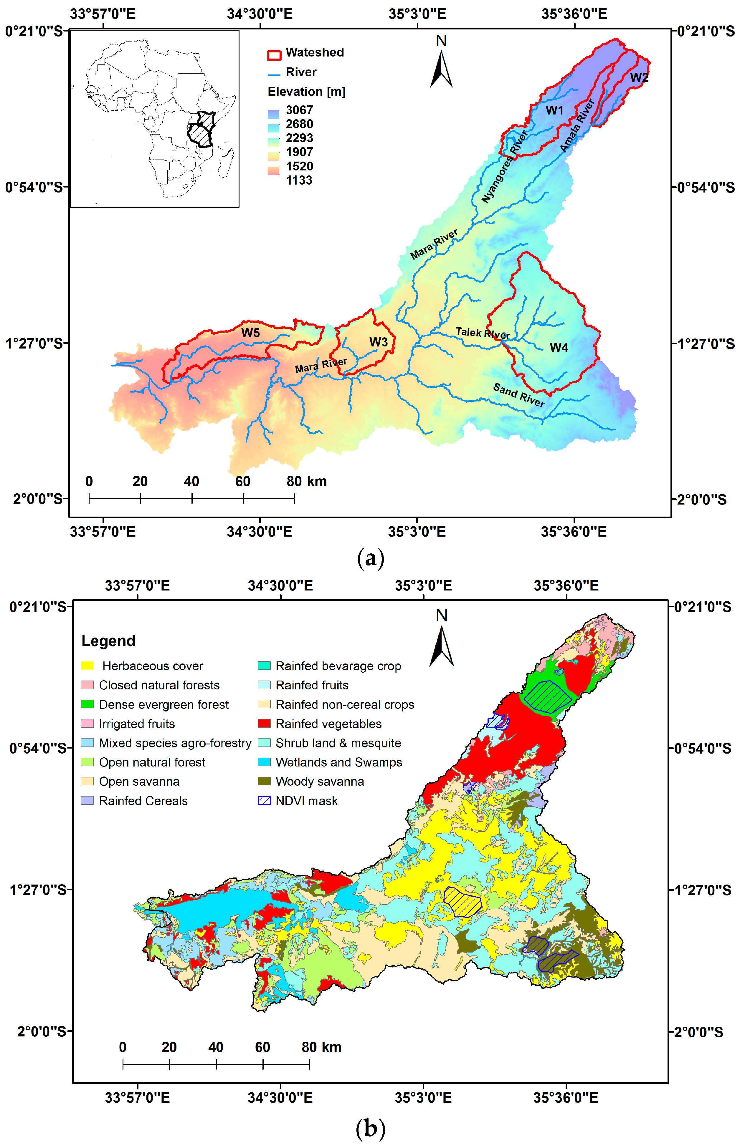
2.1. The Study Area

The Mara River basin, a transboundary river basin shared by Kenya and Tanzania, drains an area of 13,750 km2 (Figure 1a). This river originates from the forested Mau Escarpment (about 3000 meters.) and flows through agricultural and rangelands before entering the Masai-Mara Game Reserve in Kenya and the Seregenti National Park in Tanzania and, finally, joins Lake Victoria. The Amala River and the Nyangores River are the only perennial tributaries draining the head water region. The Talek River and the Sand River are the two most notable seasonal rivers stemming from the Loita Hills.
Rainfall is highly variable in the basin with the highest and lowest mean annual rainfall being 1750 mm/yr (Mau region) and 600 mm/yr (south east part), respectively [16]. This is mainly due to its equatorial location and its range of land forms, including high mountains, expansive plains and a large inland lake. The rainfall pattern in most parts of the basin is bimodal, with a short rainy season (October–December) driven by convergence and southward migration of the Intertropical Convergence Zone (ITCZ) and a long rainy season (March–May) driven by southeasterly trade winds. The mean annual temperature is approximately 25.5 °C, and in general, temperature increases southwards.
The Mara basin is endowed with significant biodiversity features through a sequence of zones from moist montane forest on the escarpment through dry upland forest to scattered woodland and then the extensive grasslands of savanna, with areas of scrub and thorn trees (Figure 1b).

2.2. Preprocessing the Forcing and Ancillary Datasets

2.2.1. The Earth Observation Products

The advancement in Earth observing systems (EOS) has been providing unprecedented comprehensive information about the Earth’s land, oceans and atmosphere, over an increasingly refined spectral resolution [18]. Terra (morning) and Aqua (afternoon) satellites carry on board the MODIS, which has the highest number of spectral bands and nearly global coverage, since 1999 and 2002, respectively [19]. MODIS land surface products are available with different levels of processing (raw to Level 4). All of the MODIS products used in this research (Table 1) are Level 3 (Version 5) in sinusoidal grid projection, whereby the necessary atmospheric and geometric corrections have been implemented. We acquired these products from the Land Processes Distributed Active Archive Center (LPDAAC) of National Aeronautics and Administration (NASA) [20].
The MOD11A1 Ts is retrieved based on the generalized split-window land surface temperature algorithm [21,22]. Wan [21] reported an accuracy better than 1 K in 39 out of 47 clear-sky cases by comparing Version 5 MODIS Ts with in situ values. This study also marked that the quantity and quality of MODIS Ts Version 5 products depend on the clear-sky conditions because of the inherent limitation of the thermal infrared remote sensing. Ts is one of the key drivers in the physics of land-surface processes, such as SEB. Previous studies highlighted the influence of the quality of Ts on the accuracy of the ET estimates from SEB [23,24]. Therefore, we used only cloud-free Ts images with quality flag 0 and/or an accuracy level within ±1 K. Given the tropical location of the study area, there are gaps in the Ts images, particularly in the mountainous region, due to cloud contamination. Consequently, a gap-filling approach was applied using the R raster package [25] in the R environment. Hereby, missing data are replaced by the mean of the neighboring (non-gap) pixels within a 3 by 3 pixel window. If no cloud-free pixels are available within a 3 by 3 pixel window, a temporal interpolation is used. This gap-filling procedure is conceptually similar to the method suggested by Weiss et al. [26] to generate spatially-continuous Enhanced Vegetation Index (EVI) and Ts data for the African continent. After the quality check and gap-filling, we obtained a total of 945 images for the period between 2002 and 2010, which assures eight images per month on average.
The MOD13A1 provide NDVI estimates at 16-day intervals. The theoretical basis of the MODIS NDVI product algorithm and validation results are detailed in Huete et al. [27]. Vegetation indices have been correlated with various vegetation parameters, such as the Leaf Area Index, the biomass, the canopy cover and the fraction of absorbed photosynthetically-active radiation (fAPAR). Furthermore, several studies showed a strong linear relationship between ET and NDVI [5,31,32,33,34,35].
As in situ ET measurements are non-existent in the study area, we used the NDVI to evaluate the SSEBop ET estimates at 16-day, monthly and annual temporal scales for various land-cover classes. We created a land cover mask for each representative land cover class (see Figure 1b), based on the Africover map [36] and Google Earth images, to reduce the likely uncertainty from mixed covers. For this analysis, we considered only pixels of MOD13A1 with reliability flag 0 for each sample land cover mask. NDVI values below 0 and NDVI values with a random increase greater than 0.4 in 16 days were rejected and then replaced by linear interpolation. Finally, to remove the remaining noise in the NDVI time series, we applied a modified iterative Savitzky–Golay filter [37] method as described by Chen et al. [38].

2.2.2. The MODIS Evapotranspiration

The MODIS global evapotranspiration product (MOD16) provides global ET estimates over vegetated areas at a 1-km spatial scale for 8-day, monthly and annual temporal resolutions. This product is based on the Penman–Monteith approach [39], as described in detail in Mu et al. [28,40]. The MOD16 algorithm uses MODIS land cover, albedo, the LAI, the fPAR, the Enhanced Vegetation Index (EVI) and a daily meteorological reanalysis dataset from NASA’s Global Modeling and Assimilation Office (GMAO, v. 4.0.0, 2004).
Recently, the improved MOD16 algorithm was applied regionally to the Nile Basin countries (MOD16-NB) to estimate ET not only for vegetated areas, but also for deserts, urban areas and inland water bodies (rivers and lakes) at a 1-km regular grid [41]. For this research, we compared the monthly and annual MOD16-NB (Table 1) data with the SSEBop estimates at various spatial scales.

2.2.3. The Gridded FLUXNET Dataset

The gridded observation-based global ET (GFET) is produced by empirically up-scaling the global network of eddy covariance measurement (FLUXNET), meteorological data and the fPAR data, among others using the model tree ensembles (MTE) [15]. The GFET data are available at 50-km spatial resolution on a monthly time scale for the period of 1982–2011 at the Max Planck Institute, Germany. Further detailed descriptions on the processing algorithm are provided in Jung et al. [15].

2.2.4. The Reanalysis Dataset

The weather variables required to compute ET0 based on Allen et al. [42] are not available in the basin. Thus, we used the Global Land Data Assimilation System (GLDAS) dataset at 3-hourly and 0.25° (~25 km) resolution. Table 1 depicts all of the GLDAS weather variables used for the ET0 calculation. The GLDAS reanalysis dataset [30] is a synthesis of various reanalysis, remote sensing and ground data, including National Oceanic and Atmospheric Administration Global Data Assimilation System (NOAA/GDAS) atmospheric fields, Climate Prediction Center (CPC) Merged Analysis of Precipitation fields (CMAP) and observation-driven shortwave and longwave radiation using the Air Force Weather Agency’s AGRicultural METeorological modeling system (AGRMET).
Initially, we computed the daily reference evapotranspiration (ET025km) based on procedures and assumptions as stated in Allen et al. [42] at the GLDAS native spatial scale. As our interest is to estimate ET at the MODIS Ts spatial scale (i.e., 1 km), the ET025km requires downscaling such that the spatial variability within 25 km is accounted for. For this purpose, we used the high resolution (i.e., 30 arc second) observation-based global climatological potential evapotranspiration (ETTZ1km) dataset of Trabucco and Zomer [43]. The ETTZ1km was produced using observed maximum and minimum temperatures (1950–2000) and elevation information based on a modified Hargreaves approach [43]. ET025km was downscaled from 25 km to 1 km as follows:
E T 0 = E T T Z 1   km E T T Z 25   km   × E T 0 25   km
Figure 2 presents the downscaled GLDAS-based daily average seasonal ET0. In general, the downscaling approach increases ET0 at the pixel level (particularly in high elevation areas) and reduces the inconsistencies in gridded global forcing [8]. The downscaled ET0 values for the head water regions are comparable with the observed ET0 values reported in Alemayehu et al. [44]. Using the high resolution observation-based global ET0 for downscaling not only improved the spatial variability, but also increased the magnitude of the downscaled ET0 by about 93 mm/yr (on average). Even though the downscaled ET0 was not evaluated against observations, the spatial variation reflects the topography well, and the temporal variations correspond with the seasonal solar energy availability pattern.

2.2.5. Satellite Rainfall

The Tropical Rainfall Measuring Mission (TRMM) product provides rainfall estimates that are important to analyze the basin hydrology at fine scales (0.25° and 3-hourly; [45]). Recently, Roy et al. [29] bias-corrected TRMM Multisatellite Precipitation Analysis (TMPA) for the Mara Basin. In this study, we used this bias-corrected product at a 4-km spatial resolution. The reader is referred to Roy et al. [29] for details on the bias-correction procedures.

2.2.6. The Land- Cover Classes

The land-cover classes for the study area were adopted from the Africover map for East Africa [17]. This map is based on expert interpretation of Landsat Thematic Mapper (TM) imagery acquired at different dates (from 1990–2004). The Land Cover Classification System (LCCS) methodology comprises 50 land-cover classes, and the classified map was validated with fieldwork [46]. For this study, the Africover classes for the Mara Basin were reclassified to 15 classes and used to aggregate the ET per land cover class (Figure 1b).

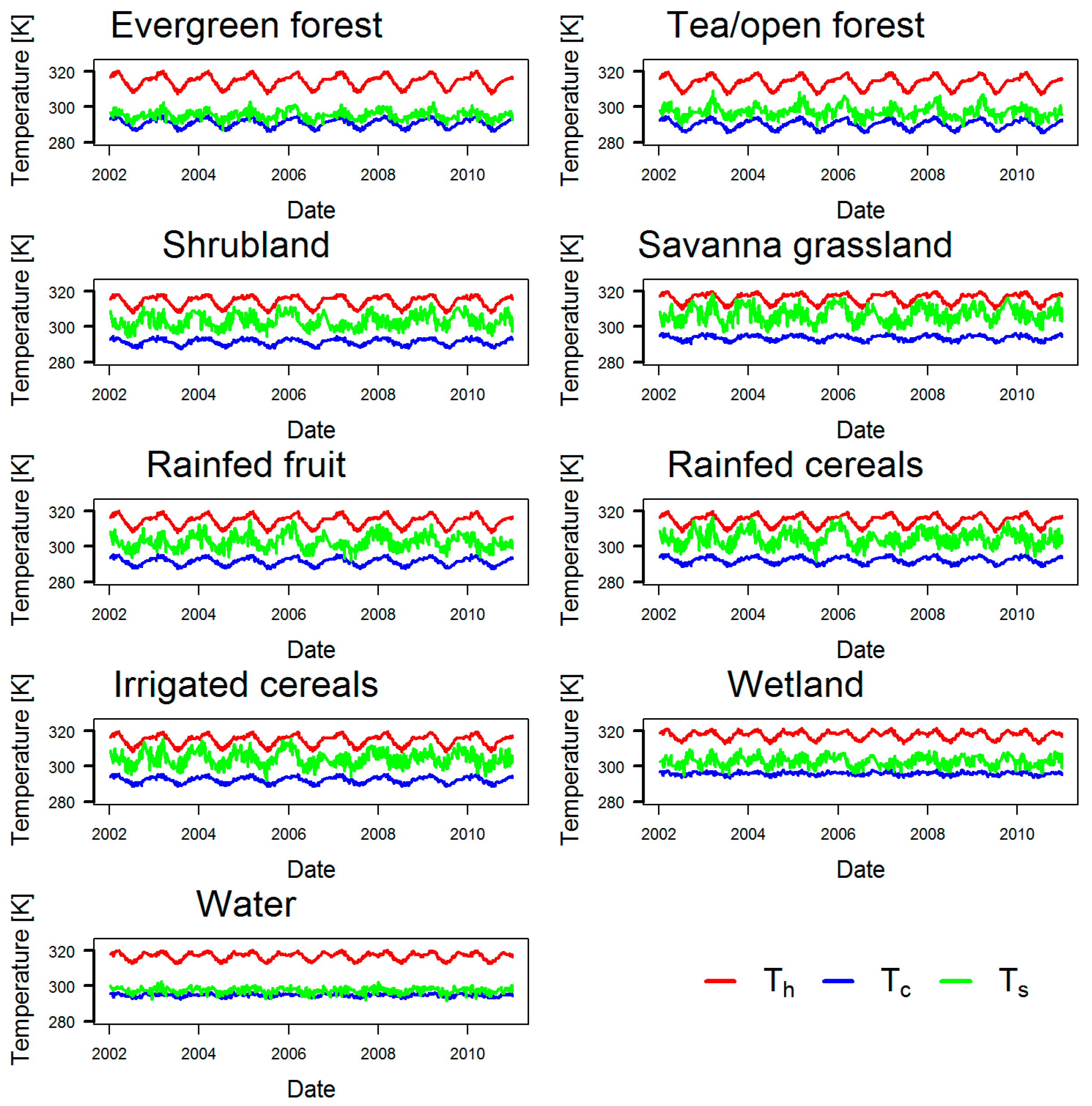
2.3. Summary of the Fundamental Principles of the SSEBop Algorithm

SSEBop is a simplified SEB algorithm that calculates ET as a fraction of the ET0, in which the ET fraction is determined using Ts and predefined hot and cold reference temperatures [9]. The ET is computed as:
E T = E T f × k × E T 0
where ET0 is the grass reference evapotranspiration for the location (mm/d); k is a coefficient that scales ET0 for an aerodynamically rough crop (-). The recommended value for k is about 1.2; however, due to the absence of a calibration dataset, we assume a value of 1.0, following the practice discussed in Senay et al. [9], and this will remain a source of potential error. The ET fraction (ETf) is computed as:
E T f = 1 ( T s T c d T )
where Ts is the land surface temperature (K); and dT is the difference between the hot reference temperature (Th) and cold reference temperature (Tc) (K).
The difference between the hot and cold reference temperatures is predefined for each location and period using a simplified climatological energy balance procedure [9]. The cold reference temperature is calculated as a fraction of the maximum daily air temperature, based on the assumption that for a given clear-sky day, the land surface would experience an ET rate equal to the potential rate for a well-watered surface (with healthy vegetation and/or soil).
T c = c × T max
Most previous studies [9,12] consider a constant calibration coefficient (c). In this study, however, we consider a seasonally-variable c, as also recommended in Senay et al. [14]. Hereby, c is determined as a quotient of Ts and maximum air temperature (Tmax) for pixels located in mixed wetland and shallow water. We note, on average, up to a 2 K reduction and 1.3 K increment of Tc during dry and wet months, respectively, when using a seasonally-varying calibration coefficient rather than a constant c (i.e., the seasonal mean).
The predefined dT is computed by solving the SEB for a bare and dry soil, whereby the latent heat flux (i.e., ET) and the soil heat flux are assumed to be 0 and the sensible heat flux (H) is assumed to be at maximum. Thus, by replacing H with the net available radiation (Rn) in the classical sensible heat flux equation, dT is equated as follows:
d T = R n × r a h ρ a × c p
where rah is the aerodynamic resistance to heat transfer from a hypothetical dry, bare surface (110 s/m), ρα is the density of air (kg/m3) and cp is the specific heat of air at constant pressure (1004 J/kg/K). The calculations of the net radiation under clear-sky conditions are based on Allen et al. [42], and the reader is referred to Senay et al. [9] for a detailed description of the SSEBop parameterization. Figure 3 shows the dynamics of the clear sky Ts, Tc and Th (i.e., Tc + dT) for selected land-cover classes from 2002–2010. It is important to note that dT, as well as the reference temperatures are unique for each period (daily in this study) and location, but the value does not vary from year to year since it is calculated under a clear-sky condition.
In the absence of cloud-free images, ET is estimated by combining ET0 and ETf from the available closest date. The maximum gap for the ETf interpolation is less than 8 days in most cases. The 8-day, 16-day, monthly and annual ET are computed as an aggregation of daily ET estimates.

2.4. Model Performance and Uncertainty Analysis Methodologies

2.4.1. Basin Scale Validation

The accuracy of SSEBop ET and MOD16-NB is validated using the only available observation-based monthly GFET from 2002–2010 (i.e., 108 months) at the basin scale. The GFET has been used to verify modeled ET across several river basins in the U.S. [11] and Europe [47]. Velpuri et al. [11] reported the reliability of this product by comparing against basin water balance ET and flux tower measurement across the U.S. In this research, the performances of monthly and annual SSEBop ET and MOD16-NB are determined based on multiple statistical measures using GFET as the reference dataset. The evaluation measures include the root mean squared error (RMSE), the percent of bias (PBIAS) and the Pearson correlation coefficient (r).

2.4.2. The MOD16-NB-Based Evaluation

The SSEBop ET estimates are compared with MOD16-NB across different spatial scales (land- cover type and basin level) and temporal scales (monthly, seasonal and annual) to explore the extent of discrepancy and/or agreement using multiple statistical metrics. Nevertheless, it should be noted that the MOD16-NB is not based on in situ measured weather variables, albeit the only public domain 1-km ET product for the study area. Further, previous validation studies [11,28,48,49,50] also revealed limitations of the product for certain land-cover classes, climate zones and elevation zones. Yet, such a comparison of ET estimates is useful to shed light on differences on ET estimates due to forcing data, model structure and its parameterization.
In addition to the error deviation measures, we use a non-parametric statistical test to assess whether the two ET estimates are similar in their means and variances. The difference between the means and the variances of SSEBop ET and MOD16-NB for each land cover class are tested using the Wilcoxon rank sum test [51] and Levene’s test [52], respectively. The hypotheses testing was carried out at the 95% confidence level.

2.4.3. The Evaluation Based on Vegetation Indices and Natural Drivers

The NDVI is a measure of canopy greenness that is linked to physiological processes, such as transpiration and photosynthesis [34,53]. Glenn et al. [53] reported linear correlations between ET and the NDVI with R2 values of 0.81 for agricultural crops and natural ecosystems. Such strong linear association between the NDVI and ET have been instrumental to predict ET at different spatial and temporal scales [31,32,33,34,35]. As such, Loukas et al. [34] noted a good agreement of the NDVI-derived ET and the ET from the water balance method for both wet and water-limiting conditions.
In this research, we use the MOD13A1 NDVI to evaluate the SSEBop estimated ET at 16-day, monthly and annual scales assuming that the magnitude and pattern of the SSEBop ET should linearly associate with the NDVI and hence serves as a proxy for the reliability of our ET estimates. Towards this, the R2 and the r are used to measure the strength of the linear relationship. The necessary steps taken to reduce the noises and errors from the NDVI time series are described in Section 3.1.
Budyko [54] hypothesized that the long-term annual evapotranspiration (ET) is primarily controlled by the available energy (i.e., climatic potential evapotranspiration ET0) and water (i.e., climatic rainfall P), whereas the landscape characteristics (soil, topography, geology, land cover, etc.) play a secondary role [55,56]. Recently, Troch et al. [55] demonstrated the existence of strong interactions between climate, vegetation and soil that lead to specific hydrologic partitioning at the watershed scale. As elaborated in Zhang et al. [56], the rational function approach developed by Fu [57] is useful in understanding the dynamic nature of catchment water balance and its intra-annual variability while considering only the primary controlling factors. In Fu’s equation (see Equation (6)) the parameter (w) represents, in a lumped way, the effects of landscape characteristics on the partitioning of P [56].
E T P = 1 + E T 0 P [ 1 + ( E T 0 P ) w ] 1 / w
Under data limited circumstances, linking the natural watershed characteristics with the dominant water balance component using Fu’s equation is not only useful to assess the consistency of the ET estimates with varying drivers, but also to scrutinize if the aggregated annual ET values are within the expected physical bounds. For this purpose, as shown in Table 2, we identified five watersheds (W1–W5) across the basin with varying landscape characteristics and climate (see Figure 1a). Therefore, we illustrate the evaporative index (i.e., ET to P) and the aridity index (i.e., ET0 to P) for these watersheds using the Budyko diagram and hence highlight their differences qualitatively. Additionally, we optimize the w parameter in Equation (6) such that watersheds with a relatively high annual ET rate will cluster around a Fu’s curve with a high w value for a similar climate [56].
1 Dominant land cover/soil; 2 Aridity Index (ET0/P).

2.4.4. The Evaluation of the Uncertainty of the SSEBop ET Estimates

Assessing the uncertainty of model simulated variables is a crucial procedure particularly for model simulation in data-scarce regions. The major sources of uncertainties include the input uncertainty, the model parameter uncertainty and the model structure uncertainty [58]. In this study, we quantified a 95% confidence interval for the mean annual ET estimates at the land cover and basin level using a non-parametric bootstrapping approach [59]. Hereby, 2000 samples were generated with replacement from the annual estimates to determine the lower (2.5%) and upper (97.5%) boundaries of the confidence interval. A similar approach has been used to assess the uncertainties of water balance terms for a catchment in East Africa [60]. The robustness of the confidence interval depends on the quality of the original sample, and therefore, we considered only annual ET estimates as (i) the SEB approach generally yields reliable estimates of ET at an annual resolution [6,7,9] and (ii) annual values eliminate any potential intra-seasonal variations in the ET estimates.

3. Results and Discussion

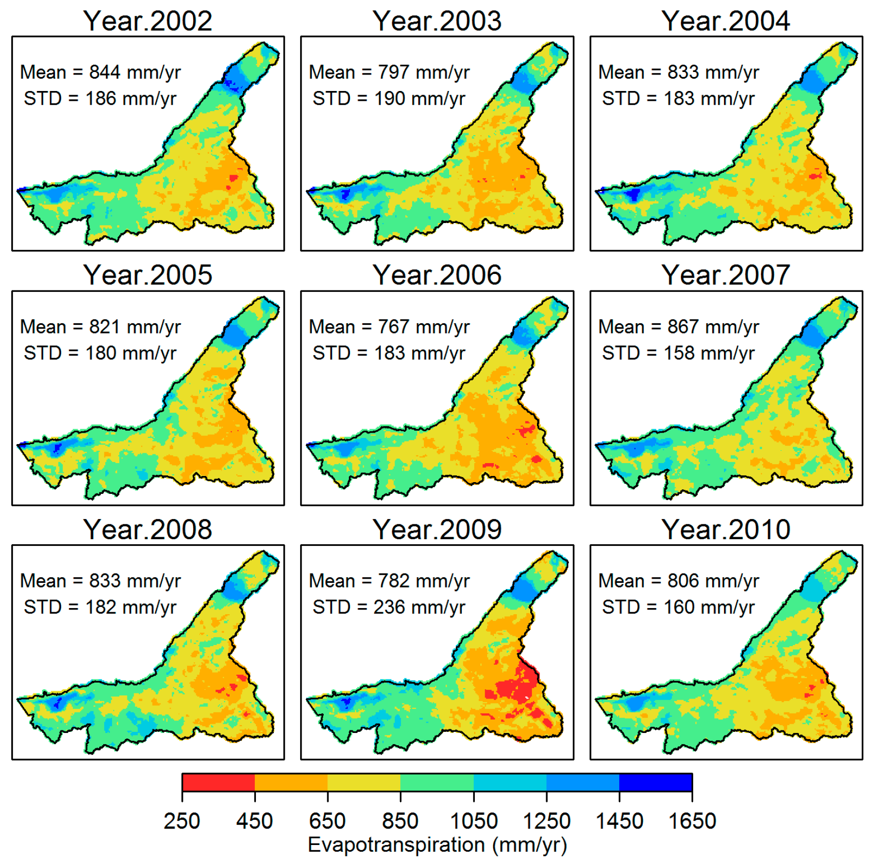
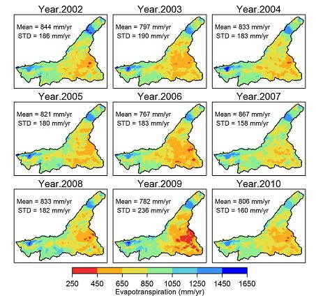
3.1. The ET Estimates at Different Temporal and Spatial Scales

The key confounding factors that control the dynamics of ET both in space and time include: elevation, soil type, land cover, weather and water availability. The Mara Basin is characterized by significant heterogeneities of the aforementioned factors and so does ET. Figure 4 presents the summary of 8-day aggregated SSEBop ET across several land-cover classes over a period of nine years. The highest and lowest 8-day median ET values are noted for areas with wetland/water cover (28.1 mm) and herbaceous covers (14.5 mm), respectively. The land-cover classes with less soil moisture variability, such as wetlands and evergreen montane forest, reveal an inter-quartile range (IQR: 6.6 mm/8-day (24% of the median) and 7.8 mm/8-day (29% of the median), respectively). Remarkably, the IQR for agriculture and herbaceous cover increases up to 52% of the median ET, suggesting that the modeled ET estimates are within the expected physical bounds. In general, the IQR for all of the land-cover classes depicts a noticeable temporal variation of ET.
Figure 5 illustrates the annual basin ET distribution at the 1-km spatial scale. It is apparent from annual ET maps that (i) ET is low in the eastern portion of the basin and (ii) the head water and the river mouth regions show consistently high ET values. At the basin scale, the nine-year mean annual ET is about 817 (±32) mm/yr; the low standard deviation (STD) indicates minimal inter-annual variability. However, as shown in Figure 5, the high STD magnitudes at the 1-km spatial scale signify the existence of significant spread in ET across the basin. Furthermore, we observe in Figure 5 that the basin experiences low annual ET values in 2006 (767 mm) and 2009 (782 mm). These estimates are consistent with the observed drought in 2005/2006, due to a short rain failure [61], and in 2009, due a delayed onset of the long rains [62] in Kenya. This suggests that the ET estimates are reliable in the sense that they are able to capture climatic variation (in this case drought).

3.2. An Evaluation of the ET Estimates
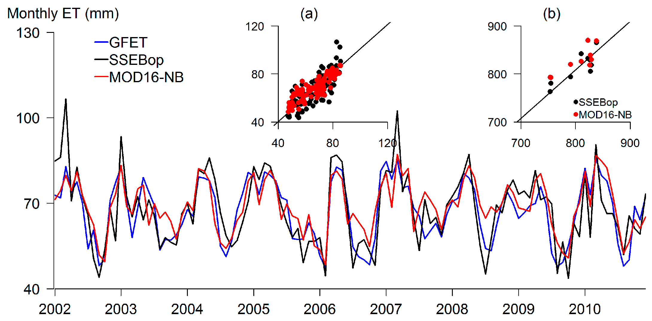
3.2.1. Validation

Figure 6 presents the comparison of basin-scale monthly SSEBop ET and MOD16-NB against the reference GFET for the period of 2002–2010. Visually, we observe that our SSEBop ET and MOD16-NB reproduced well both the magnitude and temporal dynamics of monthly GFET. This is supported by a high statistically-significant linear correlation of 0.80 (0.86), a PBIAS of 1.1% (2.8%) and an RMSE of 0.26 (0.19) mm/d between SSEBop (MOD16-NB) and GFET. As shown in Figure 6, we notice differences in monthly range among the ET products, which could be caused by differences (unlike the others, SSEBop relies on thermal) and similarities (MOD16 and GFET share inputs as noted in Velpuri et al. [11]) in approaches to show a larger dynamics that could imply more sensitivity associated with the role of Ts. Understanding the significance of these differences requires more evaluation in other hydro-climatic settings at multiple spatio-temporal scales.
At the annual scale, we note RMSE of 0.05 (0.08) mm/d and r of 0.85 (0.82) for SSEBop ET (MOD16-NB), suggesting an improvement in accuracy at coarser temporal aggregation. Furthermore, a visual inspection of Figure 5 and Figure 7 reveals a general match in the spatial pattern of ET. Overall, the validation results indicate the reasonableness of the monthly and annual SSEBop ET and MOD16-NB at the basin level for the study area.

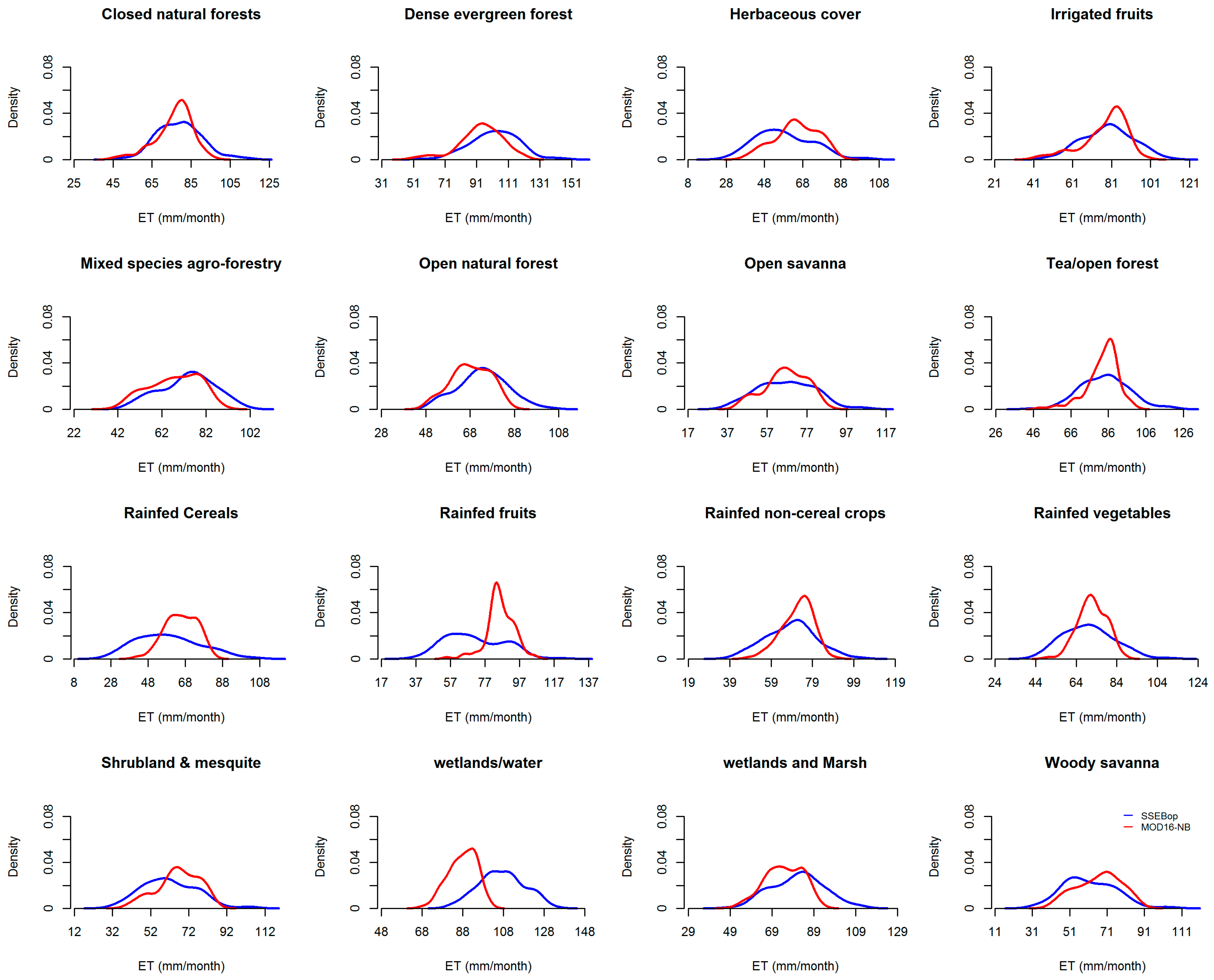
3.2.2. The Comparison of the SSEBop ET with the MOD16-NB Data

Table 3 summarizes the comparison of the SSEBop ET against the MOD16-NB data at the monthly, seasonal and annual scale for different land-cover classes. It is worth noting that the ET is aggregated using the Africover classes [17], whereas the MOD16-NB used land cover data from MODIS [28]. The average daily RMSE for the monthly ET ranges from 0.28 mm/d (open savanna) to 0.73 mm/d (wetland/water) while the largest and lowest PBIAS are about 22% (wetland/water) and 0.3% (open savanna), respectively. The linear correlation between SSEBop ET and MO16-NB across several land-cover classes ranges from 0.39–0.75 at the monthly scale and from −0.07–0.92 at the annual scale (Table 3). As shown in Table 3, the low RMSE and the relatively high correlation for the seasonal ET suggest that the two estimates agree with the seasonal pattern of ET for most of the land-cover classes.
Figure 8 and Figure 9 exhibit the discrepancies between SSEBop ET and MOD16-NB at the pixel and land cover level. MOD16-NB shows higher values of ET (up to 178 mm/yr) as compared to the SSEBop ET for agricultural cover types, as well as herbaceous cover, shrubland and woody savanna. These differences are notable with a shift and skewness of the histogram (see the third row in Figure 9). Similar observations were reported in Velpuri et al. [11]. Their comparisons with observed ET from flux towers showed a better performance of MOD16 for cropland and woody savanna cover than SSEBop, while both models underestimate ET as compared to the observations. Alemu et al. [10] also compared ET for the Nile Basin using MOD16-NB and the U.S. Geological Survey (USGS) SSEBop product for Africa and marked similar observations. On the other hand, our results show that SSEBop ET is higher than the MOD16-NB for wetland and flood plain areas and for forest covers. On average, SSEBop ET is 232 mm/yr higher than MOD16-NB for wetlands or water mixed land cover. Similarly, Alemu et al. [10] showed a large difference for wetlands in the Nile Basin. The SSEBop ET (1286 mm/yr) is comparable with the SEBAL ET estimates for wetlands and swamps in the Upper Pangani Basin (Kenya/Tanzania) (1291 mm/yr) [60], suggesting the better reliability of our estimates.
The overall modest agreements of SSEBop ET and MOD16-NB estimates (Table 3) are further corroborated by the Wilcoxon rank sum test that shows the means of the SSEBop and MOD16-NB ET values are similar at a 95% confidence level. However, Leven’s test reveals that the variances of the two ET estimates are different, partly attributed to differences both in model structure and input datasets used in MOD16-NB (mainly GMAO weather dataset 1.0° × 1.25° resolutions and MODIS fPAR/ LAI, among others) and SSEBop (mainly downscaled GLDAS weather dataset at 1 km and MODIS Ts).
The low correlation pixels are mostly noted for areas with covers such as wetland/water, mixed savanna, as well as for rainfed agriculture (i.e., vegetables, fruits and crops). This is consistent with our observation of discrepancies based on the Africover classes in Table 3 and Figure 8, indicating that the differences in the ET estimates from the two models are not so much due to the land cover-based aggregation, but rather from the ultimate difference in inputs, parameterization and model structure. This is partly in agreement with McCabe et al. [8] who reported a spread in the performance of ET models, despite using similar forcing, due to differences in parameterization and model structure. For instance, the way spatial heterogeneity (i.e., land-cover classes) is accounted for in the SSEBop and MOD16 algorithms partially explains some of the observed discrepancy in ET estimates. Whereas the MOD16 algorithm explicitly accounts for the cover heterogeneity using biome specific fPAR and LAI inputs, the SSEBop primarily depends on the Ts pixel resolution. It has been demonstrated that the accuracy of the SEB including SSEBop is influenced by the spatial scale of Ts where there is significant sub-pixel heterogeneity [1,63]. The underestimation of ET for wetlands located in a semi-arid climate by MOD16-NB can be partly attributed to the soil water stress parameterization that uses only atmospheric vapor pressure deficit (VPD) and relative humidity. This is in agreement with Hu et al. [50] who observed underestimation of global MOD16 ET estimates in a semi-arid climate even though the soil water content in the topsoil layer is high.

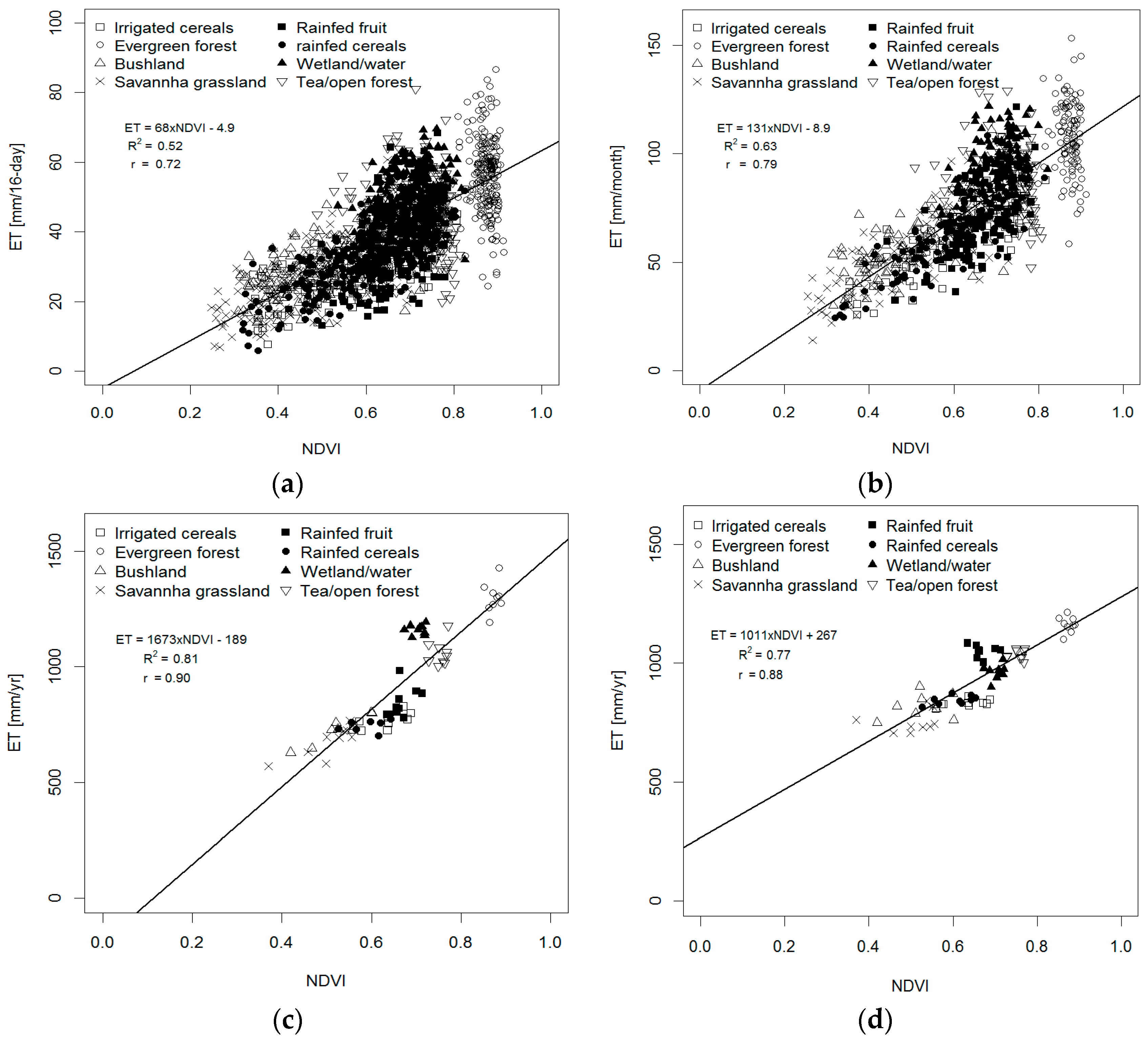
3.2.3. The NDVI-Based Evaluation

Figure 10a–c shows the relationship between the NDVI and the SSEBop ET at varying temporal aggregation levels for several land-cover classes. The SSEBop ET explains about 52%, 63% and 81% of the observed variability in the NDVI at a 16-day, monthly and annual temporal resolution, respectively. Markedly, we observe weak linear association of NDVI and ET at 16-day and monthly temporal resolution in humid highland regions and semi-arid areas with continuous moisture supply such as wetlands. This result is in agreement with Mutiga et al. [64] who noted a weak correlation between daily NDVI and SEBAL ET for elevations beyond 2100 m.a.s.l. in the upper Ewaso Ng’iro North Basin, Kenya. It is worth noting that ET shows appreciable temporal variability mainly depending on the availability of energy and transport capacity (i.e., wind) in moist regions; however, the NDVI shows less temporal variation. This highlights the weakness of the NDVI as a proxy to ET for shorter temporal scales for areas with sufficient soil moisture storage.
The interesting point to draw from Figure 10c is the existence of a clear and strong spatial and temporal pattern between the NDVI-ET relationship. A similar conclusion can be drawn from Figure 9d concerning the link between the NDVI and the MOD16-NB, even though the MOD16 algorithm uses MODIS vegetation indices as an input. This is consistent with the general understanding that NDVI is indicative of the biophysical processes, such as the transpiration and the gross primary productivity [31,32,53]. Therefore, the strong empirical relationship of NDVI and ET that encompasses several land-cover classes at an annual level is particularly attractive to estimate the annual ET in data-scarce basins, as suggested in Loukas et al. [34].

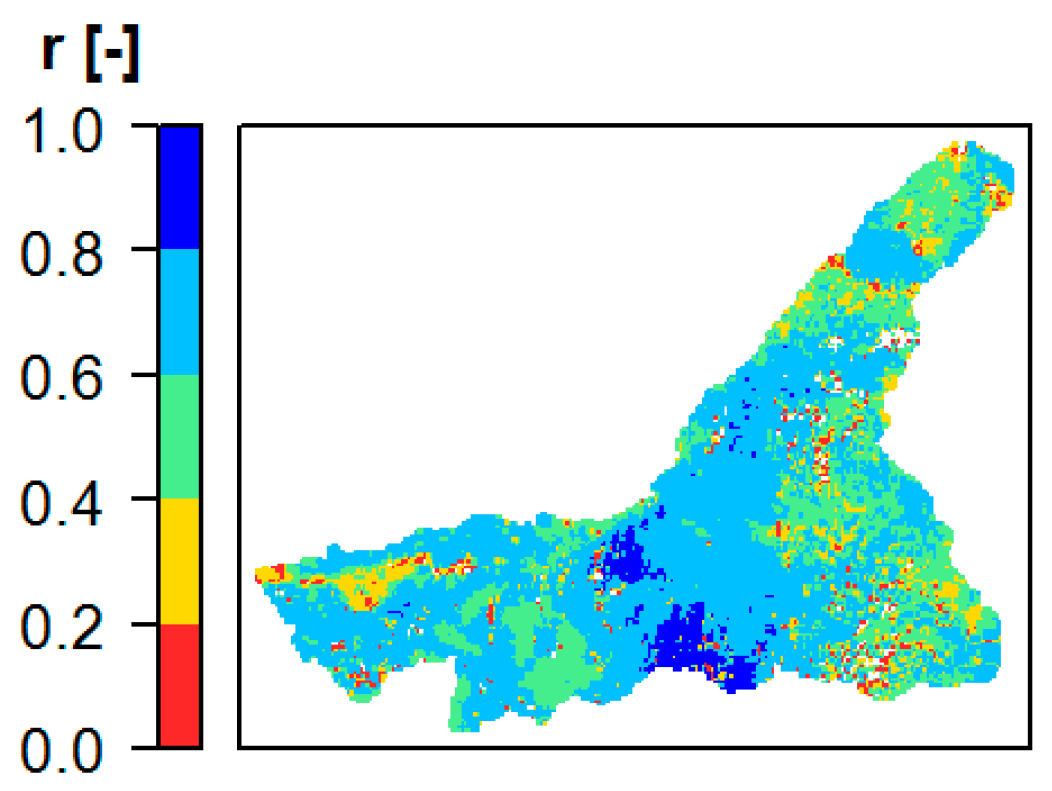
3.2.4. The Consistency of the ET Estimates across the Basin

Due to the absence of in situ ET measurements in the study area, we investigated the reasonableness of the SSEBop ET estimates by comparing with other MODIS-based products (i.e., MOD16-NB and NDVI) and GFET. The results obtained are encouraging. Furthermore, we evaluated SSEBop ET by plotting watershed average ET values in the Budyko diagram. Figure 11 illustrates the scatter plot of the evaporative index (ET to P) versus the aridity index (ET0 to P) across five watersheds, ranging from humid to semi-arid climates. It can be observed that the watersheds clustered close to Fu’s curve [57] with w of 2.7 tend to experience a high ET rate. Two groups of clusters consisting of Cluster 1 (W1, W2 and W5 with AI: 0.9–1.2); and Cluster 2 (W3 and W4 with AI: 1.4–2.1) are identified in the scatter diagram. Forest-dominated semi-humid watersheds and wetlands follow the Fu’s curve of w equal to 2.7 (Cluster 1), and grassland-dominated semi-arid watersheds follow the Fu’s curve of w equal to 1.9 (Cluster 2). The relative positioning of the clusters makes physical sense and is in line with the hydro-climatic and landscape characteristics of the watersheds (see Table 2), indicating the reliability of the SSEBop ET. Therefore, the Budyko diagram analysis and fitting the Fu’s w parameter reinforce the consistency of our results with the primary and secondary controlling factors, albeit using downscaled GLDAS-based forcing.
Recently, McCabe et al. [8] observed poor performances across all ET models (SEBS, Global Land Evaporation Model Amsterdam (GLEAM), Priestley-Taylor Jet Propulsion Laboratory (PT-JPL) and Penman-Monteith-based Mu (PM-Mu) that are forced by gridded global data in reproducing tower-based ET across several biome and climate zones. According to their analyses, the poor performances were mainly attributed to internal inconsistencies within the gridded forcing data, and yet, the ET models with fewer input requirements were less sensitive. We believe that the consistent ET estimates noted in our study at several spatial and temporal scales could be partly attributed to the downscaling of the GLDAS-based ET025km using observation-based ETTZ1km. Furthermore, the minimal model parameterization requirements of the SSEBop and the improvements on cold reference temperature (Tc) estimation might have contributed to the favorable results obtained. This has been depicted by a relatively strong correlation (r = 0.81) between the SSEBop ET and NDVI across several land-cover classes in the Mara Basin. The good correlations obtained in this study are stronger than the correlations reported for similar land covers in Alemu et al. [10] in the Nile Basin, using a similar SSEBop algorithm.

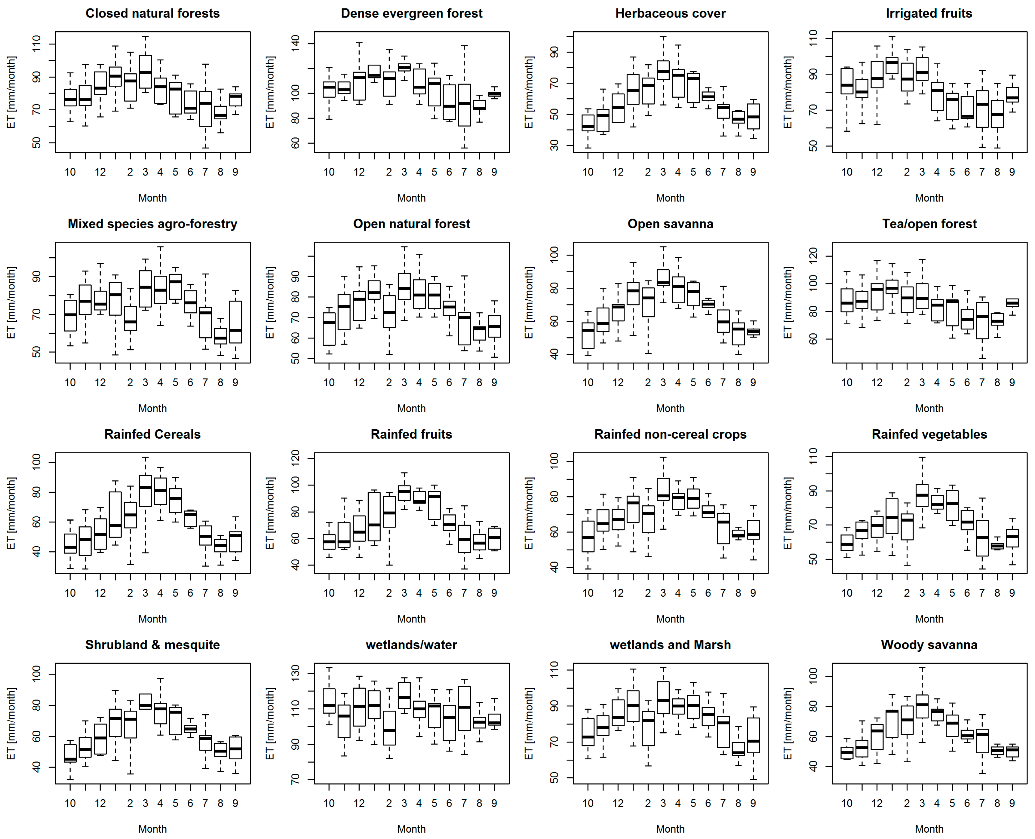
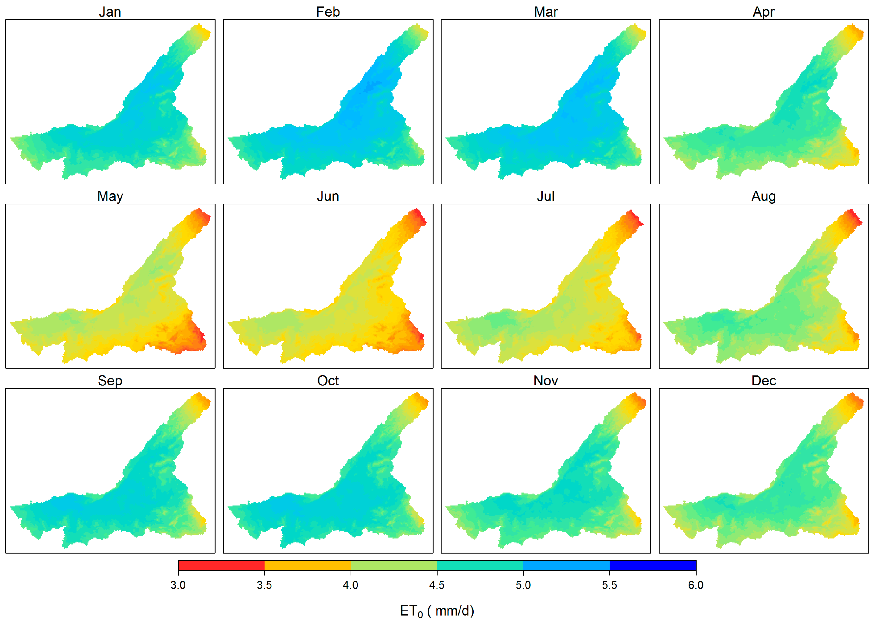
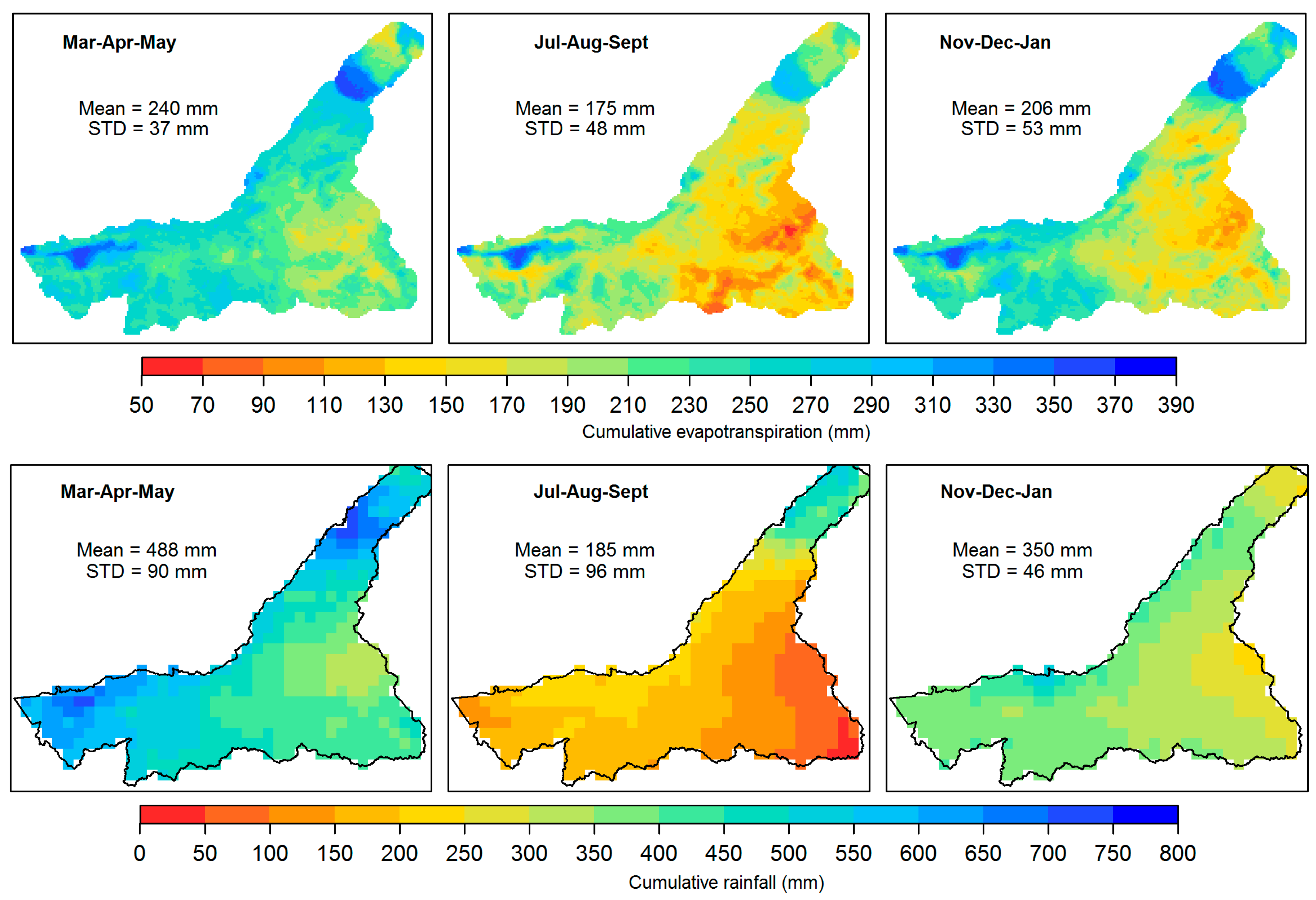
3.3. Seasonality of ET

The rainfall (and hence soil moisture) distribution is one of the main governing factors of the seasonality and spatial variability of ET. In this basin, the water year that is based on the rainfall seasonality starts on 1 October and ends on 30 September [16]. Figure 12 illustrates the monthly variability of ET in the Mara Basin. The figure shows that ET is high from October–May, due to the availability of energy and soil moisture during this period. On the other hand, we note a relatively low ET during the dry season months (June–September). However, the land-cover classes located in the humid part of the basin, such as evergreen forest and tea/open forest, show less seasonality since there is ample rainfall throughout the year. Additionally, for wetlands and marsh covers, we observe less monthly variability as there is a continuous supply of water from the Mara River and Lake Victoria. In conclusion, the SSEBop ET estimates reflect fairly well the seasonal rainfall distribution pattern in the basin.
Figure 13 presents the aggregated ET (upper row) and rainfall (bottom row) during the main rainy season (March–May), the dry season (July–September) and the small rainy season (November–January) at 1- and 4-km scales, respectively. The seasonally-aggregated ET maps show not only the high heterogeneity of ET, but also its intra-annual variations that fairly match the rainfall patterns. The cumulated ET exceeds the cumulative rainfall for the dry season months (see Figure 13). This is ascribed to the availability soil moisture supply after the main rainy season and the water extraction by deep rooted vegetation. Generally, our results indicate that the eastern portion of the catchment has low ET fluxes, which is consistent with the low rainfall input and sparse vegetation cover in that part of the basin.

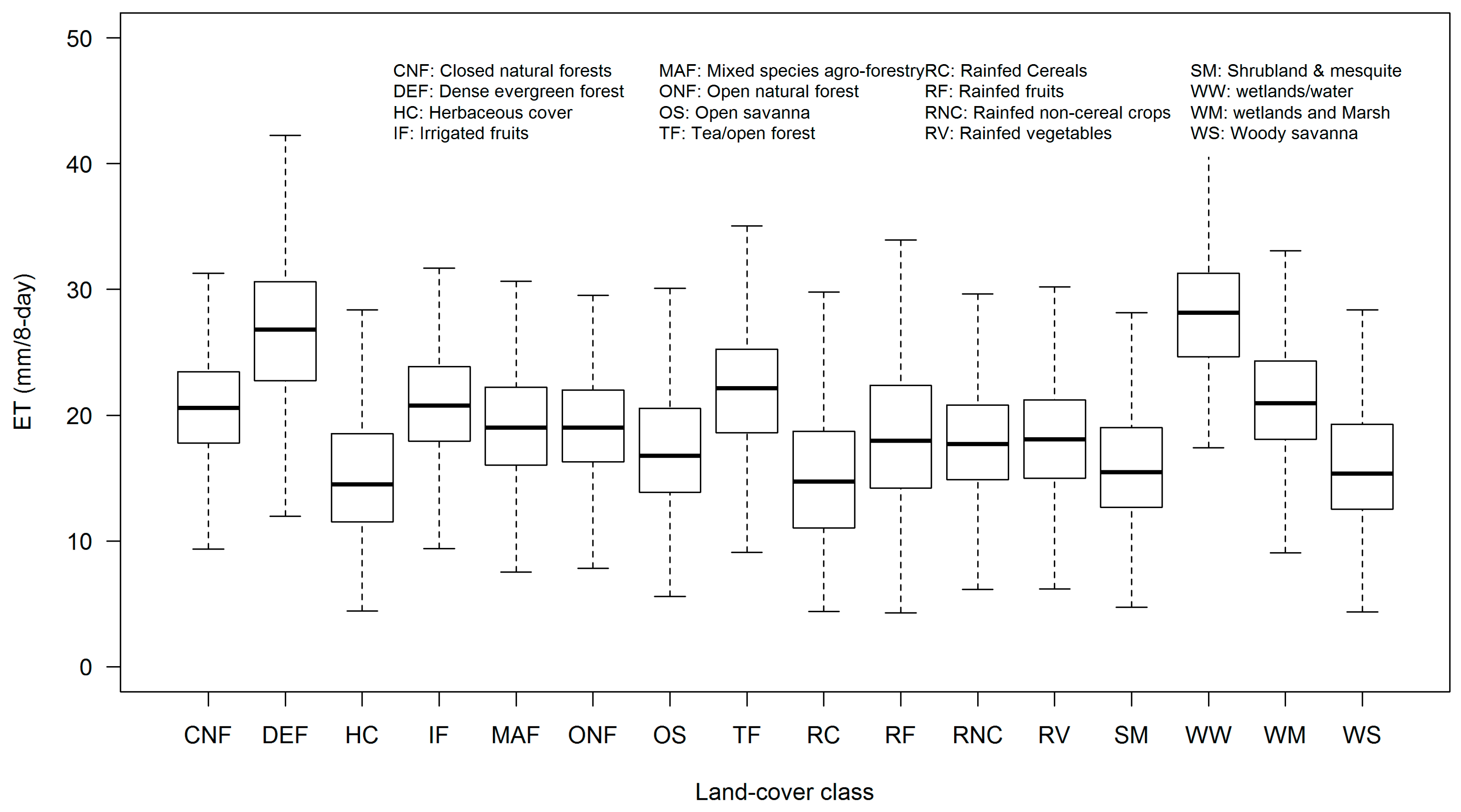
3.4. The Annual ET (Water Use) by Land Cover

Table 4 presents the mean annual SSEBop ET (i.e., the water use) and rainfall for different land-cover classes. On average, dense evergreen forest (1228 (±59) mm/yr) and wetlands (1286 (±44) mm/yr) are the highest water consumers, whereas herbaceous cover (698 (±46) mm/yr) and rainfed cereals (706 (±69) mm/yr) are the lowest consumers. The basin average water use is about 817(±32) mm/yr and accounts for 66% of the rainfall. Unlike what is the case for rainfall, the STD values for the annual ET for the different land-cover classes are low, thus suggesting a minimal inter-annual variability (Table 4). The intra-annual variability is, however, high.

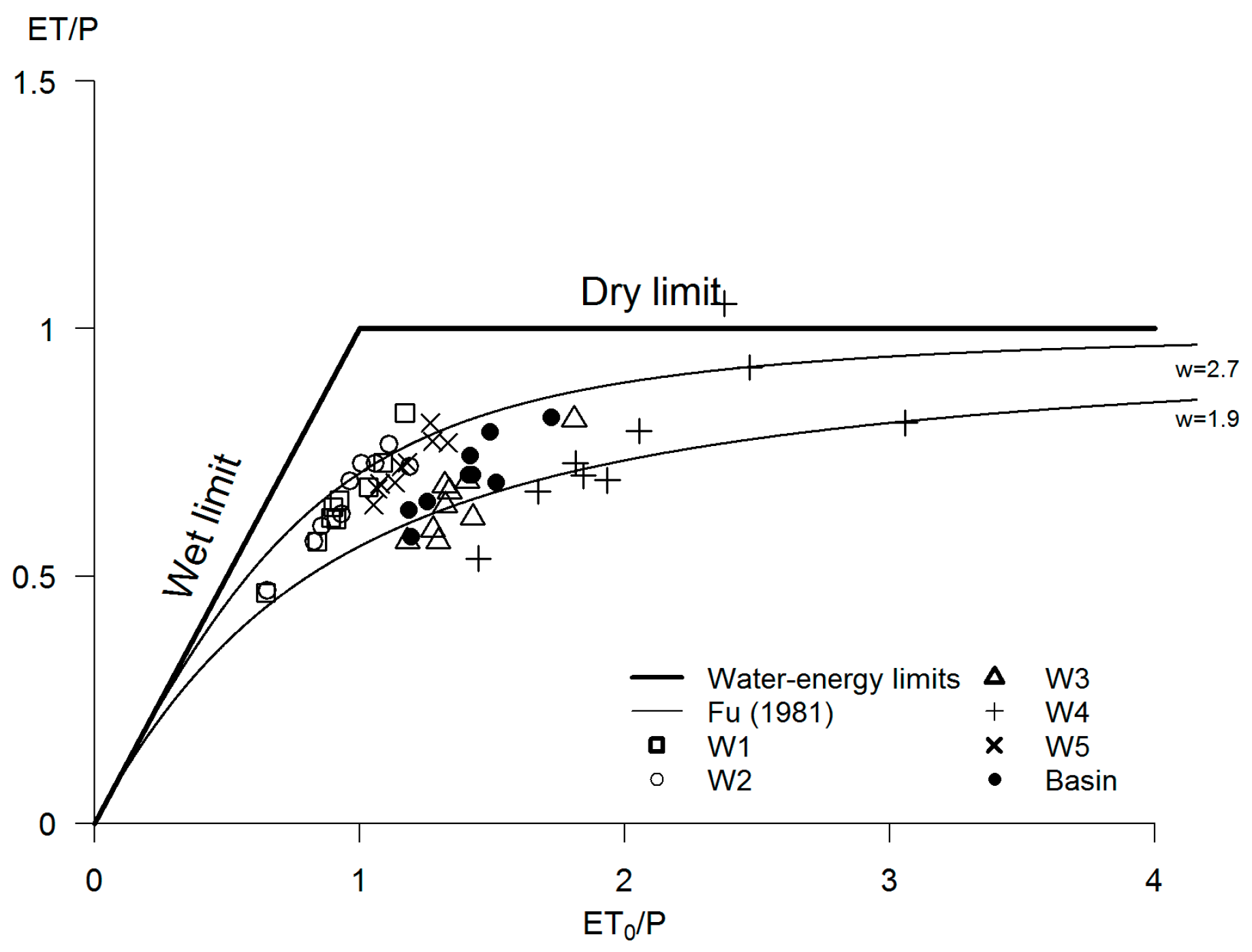
3.5. The Assessment of the Uncertainties on the ET Estimates

It is imperative to assess the uncertainties of the ET estimates as there are inherent sources of uncertainty related to input data and parameterization of the SSEBop algorithm.
As shown in Table 4 (Column 6), the 95% confidence interval ranges from 3–12% (of the mean annual ET) across different land-cover classes. Of all of the land-cover classes, agricultural land cover shows a relatively high variability (wider confidence interval) on the mean annual ET estimates. As discussed in Section 3.2.1, this is perhaps attributed to the limitation of the coarse (1 km) spatial scale of MODIS Ts to capture the spatial variability of Ts as marked in Krishnan et al. [65] and McCabe et al. [63] since agriculture in this basin is mainly the plot scale. Additionally, the year-to-year variation in types of crops growing in the field might also contribute to the wider confidence interval. The 95% confidence interval for basin mean annual SSEBop ET estimates is 39 mm/yr, which is comparable with 42 mm/yr using the GFET dataset. Overall, uncertainties in the mean annual ET from this study are similar with the reported uncertainties in Kiptala et al. [60] using SEBAL in the Upper Pangani River Basin (Kenya/Tanzania) and with other published validation results [11]. This indicates the reliability of the ET estimates derived in this study for various hydrological applications.

4. Conclusions

This paper demonstrated how to effectively estimate and evaluate spatially-distributed and temporally-varying ET in data-scarce regions. Our main objective is to map ET (1 km/8-day) using data from the Moderate Resolution Imaging Spectroradiometer (MODIS) land surface temperature (Ts) and from the Global Land Data Assimilation System (GLDAS) weather dataset based on the Operational Simplified Surface Energy Balance (SSEBop) algorithm in the Mara Basin (Kenya/Tanzania). We validate the SSEBop ET estimates and the regional MODIS evapotranspiration for the Nile countries (MOD16-NB) using globally-gridded flux tower measurements network monthly ET (GFET) [15] at the basin scale. Additionally, the SSEBop ET estimates were inter-compared and evaluated using the MOD16-NB and MODIS Normalized Vegetation Index (NDVI) at different spatial and temporal scales.
Our results show that ET in the study area is highly variable spatially and intra-annually. The land-cover classes with low variability in soil moisture reveal an inter-quartile range (IQR), e.g., 6.6 mm/8-day (24% of the median) for wetlands and 7.8 mm/8-day (29% of the median) for evergreen montane forest. Remarkably, the IQR for agriculture and herbaceous cover increases up to 52% of the median ET, suggesting the modeled ET estimates are within the expected physical bounds. On average, the basin-wide ET is about 817 (±32) mm/yr, or 66% of the rainfall.
The basin scale validation using nine-years of monthly GFET data reveals that our ET is able to explain 64% of the variance in GFET, while the MOD16-NB explains 72%. Additionally, we observe 1.1% and 2.8% percent of bias (PBIAS) for SSEBop ET and MOD16-NB, respectively, indicating a good reliability in the ET estimates. Notwithstanding the comparable performance of SSEBop ET and MOD16-NB in reproducing the basin-level GFET, we note high discrepancies between SSEBop ET and MOD16-NB for wetlands and forest (with MOD16-NB being up to 232 mm/yr lower) and rainfed agriculture (with SSEBop ET being up to 178 mm/yr lower). The former differences are partly attributed to the soil water stress parameterization in the MOD16-NB that uses the atmospheric vapor pressure deficit (VPD) and the relative humidity, particularly for the wetland located in a semi-arid climate; whereas the latter could be associated with the limitation of the 1-km scale MODIS Ts (i.e., one of the major input to SSEBop), as also noted in McCabe et al. [63] and Krishnan et al. [65], to capture the spatial variability of Ts where there is significant sub-pixel heterogeneity.
SSEBop ET explains about 52%, 63% and 81% of the observed variability of the NDVI at 16-day, monthly and annual temporal resolution, respectively, using several representative land-cover classes. Our results also show a good consistency in annual ET estimates by reflecting the underlying primary (i.e., availability of water and energy) and secondary (i.e., soil, topography, geology, land cover, etc.) controlling factors across the basin. The consistent and fair performance of the SSEBop ET can be related to the use of a seasonally-varying calibration coefficient to determine the cold reference temperature (i.e., improved parameterization) and improvements on the quality of the forcing ET0 data (i.e., improved forcing consistency). Overall, the uncertainty on the mean annual ET, as calculated by us on the land cover level, is less than 12%. This is comparable with the results of Kiptala et al. [60] who used SEBAL data in the Upper Pangani River Basin (Kenya/Tanzania) and other published validation results [11].
The strong empirical relationship developed in this study between ET and NDVI using representative land cover sites at an annual scale can be used to compute basin average ET with operational NDVI information. This is particularly interesting for water balance analysis and hydrological model parameterization, as in situ hydro-meteorological stations are scarce.
The methodological framework developed in this study, mapping ET using Earth observation products and global gridded weather data can be applied elsewhere in the world where observed hydro-meteorological variables are limited.

Acknowledgments

The authors would like to thank NASA for making the remotely-sensed products and reanalysis weather dataset publicly available for scientific research. We also would like to thank Dr. Manohar Velpuri, scientist at USGS, for sharing GFET data acquired from MPI through Dr. Martin Jung. We also would like to thank Thirthankar Roy, PhD candidate at the University of Arizona, for providing bias-corrected satellite rainfall. The constructive comments and suggestions from four anonymous reviewers are very much appreciated. Alemayehu’s site visit was made possible with funding from Mau Mara Serengeti (MaMaSe) Sustainable Water Initiative (http://mamase.org/). Senay acknowledges partial funding provided by NASA Award Number NNX14AD30G for his time. Any use of trade, firm, or product names is for descriptive purposes only and does not imply endorsement by the US Government.

Author Contributions

Tadesse Alemayehu conceived of, designed, analyzed and wrote the paper. Ann van Griensven supervised the research and contributed to the paper. Gabriel Senay contributed ideas during analysis and interpretation. Willy Bauwens contributed to discussions and reviewed the paper.

Conflicts of Interest

The authors declare no conflict of interest.

References

  1. Anderson, M.C.; Allen, R.G.; Morse, A.; Kustas, W.P. Use of Landsat thermal imagery in monitoring evapotranspiration and managing water resources. Remote Sens. Environ. 2012, 122, 50–65. [Google Scholar] [CrossRef]
  2. Bastiaanssen, W.G.M.; Noordman, E.J.M.; Pelgrum, H.; Davids, G.; Thoreson, B.P.; Allen, R.G. SEBAL Model with Remotely Sensed Data to Improve Water-Resources Management under Actual Field Conditions. J. Irrig. Drain. Eng. 2005, 131, 85–93. [Google Scholar] [CrossRef]
  3. Allen, R.G.; Pereira, L.S.; Howell, T.A.; Jensen, M.E. Evapotranspiration information reporting: II. Recommended documentation. Agric. Water Manag. 2011, 98, 921–929. [Google Scholar] [CrossRef]
  4. Allen, R.G.; Tasumi, M.; Morse, A.; Trezza, R.; Wright, J.L.; Bastiaanssen, W.; Kramber, W.; Lorite, I.; Robison, C.W. Satellite-Based Energy Balance for Mapping Evapotranspiration with Internalized Calibration (METRIC)—Applications. J. Irrig. Drain. Eng. 2007, 133, 395–406. [Google Scholar] [CrossRef]
  5. Kalma, J.D.; McVicar, T.R.; McCabe, M.F. Estimating Land Surface Evaporation: A Review of Methods Using Remotely Sensed Surface Temperature Data. Surv. Geophys. 2008, 29, 421–469. [Google Scholar] [CrossRef]
  6. Gowda, P.H.; Chavez, J.L.; Colaizzi, P.D.; Evett, S.R.; Howell, T.A.; Tolk, J.A. ET mapping for agricultural water management: Present status and challenges. Irrig. Sci. 2008, 26, 223–237. [Google Scholar] [CrossRef]
  7. Karimi, P.; Bastiaanssen, W.G.M. Spatial evapotranspiration, rainfall and land use data in water accounting—Part 1: Review of the accuracy of the remote sensing data. Hydrol. Earth Syst. Sci. 2015, 19, 507–532. [Google Scholar] [CrossRef]
  8. McCabe, M.F.; Ershadi, A.; Jimenez, C.; Miralles, D.G.; Michel, D.; Wood, E.F. The GEWEX LandFlux project: Evaluation of model evaporation using tower-based and globally gridded forcing data. Geosci. Model Dev. 2016, 9, 283–305. [Google Scholar] [CrossRef]
  9. Senay, G.B.; Bohms, S.; Singh, R.K.; Gowda, P.H.; Velpuri, N.M.; Alemu, H.; Verdin, J.P. Operational Evapotranspiration Mapping Using Remote Sensing and Weather Datasets: A New Parameterization for the SSEB Approach. JAWRA J. Am. Water Resour. Assoc. 2013, 49, 577–591. [Google Scholar] [CrossRef]
  10. Alemu, H.; Senay, G.; Kaptue, A.; Kovalskyy, V. Evapotranspiration Variability and Its Association with Vegetation Dynamics in the Nile Basin, 2002–2011. Remote Sens. 2014, 6, 5885–5908. [Google Scholar] [CrossRef]
  11. Velpuri, N.M.; Senay, G.B.; Singh, R.K.; Bohms, S.; Verdin, J.P. A comprehensive evaluation of two MODIS evapotranspiration products over the conterminous United States: Using point and gridded FLUXNET and water balance ET. Remote Sens. Environ. 2013, 139, 35–49. [Google Scholar] [CrossRef]
  12. Bhattarai, N.; Shaw, S.B.; Quackenbush, L.J.; Im, J.; Niraula, R. Evaluating five remote sensing based single-source surface energy balance models for estimating daily evapotranspiration in a humid subtropical climate. Int. J. Appl. Earth Obs. Geoinf. 2016, 49, 75–86. [Google Scholar] [CrossRef]
  13. Bastiaanssen, W.; Karimi, P.; Rebelo, L.-M.; Duan, Z.; Senay, G.; Muttuwatte, L.; Smakhtin, V. Earth Observation Based Assessment of the Water Production and Water Consumption of Nile Basin Agro-Ecosystems. Remote Sens. 2014, 6, 10306–10334. [Google Scholar] [CrossRef]
  14. Senay, G.B.; Schauer, M.; Friedrichs, M.; Velpuri, M.N.; Singh, R.K. Satellite-based Water Use Dynamics Using Historical Landsat Data (1984–2014) in the Southwestern United States. Remote Sens. Environ. 2017. [Google Scholar] [CrossRef]
  15. Jung, M.; Reichstein, M.; Margolis, H.A.; Cescatti, A.; Richardson, A.D.; Arain, M.A.; Arneth, A.; Bernhofer, C.; Bonal, D.; Chen, J.; et al. Global patterns of land-atmosphere fluxes of carbon dioxide, latent heat, and sensible heat derived from eddy covariance, satellite, and meteorological observations. J. Geophys. Res. 2011, 116, G00J07. [Google Scholar] [CrossRef]
  16. Water Resources and Energy Management (WREM) International Inc. Mara River Basin Monograph, Mara River Basin Transboundary Integrated Water Resources Management and Development Project, Final Technical Report; WREM International Inc.: Atlanta, GA, USA, 2008.
  17. FAO Africover Regional Land Cover Database. Available online: http://www.africover.org (accessed on 10 June 2014).
  18. Tralli, D.M.; Blom, R.G.; Zlotnicki, V.; Donnellan, A.; Evans, D.L. Satellite remote sensing of earthquake, volcano, flood, landslide and coastal inundation hazards. ISPRS J. Photogramm. Remote Sens. 2005, 59, 185–198. [Google Scholar] [CrossRef]
  19. Justice, C.O.; Townshend, J.R.G.; Vermote, E.F.; Masuoka, E.; Wolfe, R.E.; Saleous, N.; Roy, D.P.; Morisette, J.T. An overview of MODIS Land data processing and product status. Remote Sens. Environ. 2002, 83, 3–15. [Google Scholar] [CrossRef]
  20. LPDAAC Land Processes Distributed Active Archive Center (LPDAAC) of NASA. Available online: https://lpdaac.usgs.gov/data_access/data_pool (accessed on 5 December 2014).
  21. Wan, Z. New refinements and validation of the collection-6 MODIS land-surface temperature/emissivity product. Remote Sens. Environ. 2008, 140, 36–45. [Google Scholar] [CrossRef]
  22. Wan, Z.; Zhang, Y.; Zhang, Q.; Li, Z. Validation of the land-surface temperature products retrieved from Terra Moderate Resolution Imaging Spectroradiometer data. Remote Sens. Environ. 2002, 83, 163–180. [Google Scholar] [CrossRef]
  23. Van der Kwast, J.; Timmermans, W.; Gieske, A.; Su, Z.; Olioso, A.; Jia, L.; Elbers, J.; Karssenberg, D.; de Jong, S. Evaluation of the Surface Energy Balance System (SEBS) applied to ASTER imagery with flux-measurements at the SPARC 2004 site (Barrax, Spain). Hydrol. Earth Syst. Sci. 2009, 13, 1337–1347. [Google Scholar] [CrossRef]
  24. Chen, M.; Senay, G.B.; Singh, R.K.; Verdin, J.P. Uncertainty analysis of the Operational Simplified Surface Energy Balance (SSEBop) model at multiple flux tower sites. J. Hydrol. 2016, 536, 384–399. [Google Scholar] [CrossRef]
  25. Hijmans, R.J. Raster: Geographic Analysis and Modeling with Raster Data. R Package Version 2.2. Available online: https://cran.r-project.org/web/packages/raster/ (accessed on 20 April 2017).
  26. Weiss, D.J.; Atkinson, P.M.; Bhatt, S.; Mappin, B.; Hay, S.I.; Gething, P.W. An effective approach for gap-filling continental scale remotely sensed time-series. ISPRS J. Photogramm. Remote Sens. 2014, 98, 106–118. [Google Scholar] [CrossRef] [PubMed]
  27. Huete, A.; Didan, K.; Miura, T.; Rodriguez, E.P.; Gao, X.; Ferreira, L.G. Overview of the radiometric and biophysical performance of the MODIS vegetation indices. Remote Sens. Environ. 2002, 83, 195–213. [Google Scholar] [CrossRef]
  28. Mu, Q.; Zhao, M.; Running, S.W. Improvements to a MODIS global terrestrial evapotranspiration algorithm. Remote Sens. Environ. 2011, 115, 1781–1800. [Google Scholar] [CrossRef]
  29. Roy, T.; Serrat-Capdevila, A.; Gupta, H.; Valdes, J. A platform for probabilistic Multimodel and Multiproduct Streamflow Forecasting. Water Resour. Res. 2017, 53, 376–399. [Google Scholar] [CrossRef]
  30. Rodell, M.; Houser, P.R.; Jambor, U.; Gottschalck, J.; Mitchell, K.; Meng, C.-J.; Arsenault, K.; Cosgrove, B.; Radakovich, J.; Bosilovich, M.; et al. The Global Land Data Assimilation System. Bull. Am. Meteorol. Soc. 2004, 85, 381–394. [Google Scholar] [CrossRef]
  31. Szilagyi, J. Can a vegetation index derived from remote sensing be indicative of areal transpiration? Ecol. Modell. 2000, 127, 65–79. [Google Scholar] [CrossRef]
  32. Szilagyi, J.D.; Rundquist, C.; Gosselin, D.C. NDVI relationships to monthly evaporation. Geophys. Res. Lett. 1998, 25, 1753–1756. [Google Scholar] [CrossRef]
  33. Glenn, E.P.; Doody, T.M.; Guerschman, J.P.; Huete, A.R.; King, E.A.; McVicar, T.R.; Van Dijk, A.I.J.M.; Van Niel, T.G.; Yebra, M.; Zhang, Y. Actual evapotranspiration estimation by ground and remote sensing methods: the Australian experience. Hydrol. Process. 2011, 25, 4103–4116. [Google Scholar] [CrossRef]
  34. Loukas, A.; Vasiliades, L.; Domenikiotis, C.; Dalezios, N.R. Basin-wide actual evapotranspiration estimation using NOAA/AVHRR satellite data. Phys. Chem. Earth Parts A/B/C 2005, 30, 69–79. [Google Scholar] [CrossRef]
  35. Nagler, P.L.; Glenn, E.P.; Nguyen, U.; Scott, R.L.; Doody, T. Estimating riparian and agricultural actual evapotranspiration by reference evapotranspiration and MODIS enhanced vegetation index. Remote Sens. 2013, 5, 3849–3871. [Google Scholar] [CrossRef]
  36. Jansen, L.J.M.; Di Gregorio, A. Land-use data collection using the “land cover classification system”: Results from a case study in Kenya. Land Use Policy 2003, 20, 131–148. [Google Scholar] [CrossRef]
  37. Savitzky, A.; Golay, M.J.E. Smoothing and Differentiation of Data by Simplified Least Squares Procedures. Anal. Chem. 1964, 36, 1627–1639. [Google Scholar] [CrossRef]
  38. Chen, J.; Jönsson, P.; Tamura, M.; Gu, Z.; Matsushita, B.; Eklundh, L. A simple method for reconstructing a high-quality NDVI time-series data set based on the Savitzky–Golay filter. Remote Sens. Environ. 2004, 91, 332–344. [Google Scholar] [CrossRef]
  39. Monteith, J.L. Evaporation and the environment. In The State and Movement of Water in Living Organisms; Cambridge University Press: Cambridge, UK, 1965; pp. 205–234. [Google Scholar]
  40. Mu, Q.; Heinsch, F.A.; Zhao, M.; Running, S.W. Development of a global evapotranspiration algorithm based on MODIS and global meteorology data. Remote Sens. Environ. 2007, 111, 519–536. [Google Scholar] [CrossRef]
  41. MOD16-NBI Nile Basin Actual Evapo-Transpiration Based on Improved MOD16 Algorithm. Nile Informations System. Available online: http://nileis.nilebasin.org/node/147065 (accessed on 10 October 2014).
  42. Allen, R.G.; Pereira, L.S.; Raes, D.; Smith, M. Crop Evapotranspiration-Guidelines for Computing Crop Water Requirements; FAO Irrigation and Drainage Paper 56; FAO: Rome, Italy, 1998. [Google Scholar]
  43. Trabucco, A.; Zomer, R.J. Global Aridity Index (Global-Aridity) and Global Potential Evapo-Transpiration (Global-PET) Geospatial Database. Available online: www.cgiar-csi.org/data (accessed on 20 July 2014).
  44. Alemayehu, T.; van Griensven, A.; Bauwens, W. Evaluating CFSR and WATCH Data as Input to SWAT for the Estimation of the Potential Evapotranspiration in a Data-Scarce Eastern-African Catchment. J. Hydrol. Eng. 2015, 21, 05015028. [Google Scholar] [CrossRef]
  45. Huffman, G.J.; Bolvin, D.T.; Nelkin, E.J.; Wolff, D.B.; Adler, R.F.; Gu, G.; Hong, Y.; Bowman, K.P.; Stocker, E.F. The TRMM Multisatellite Precipitation Analysis (TMPA): Quasi-Global, Multiyear, Combined-Sensor Precipitation Estimates at Fine Scales. J. Hydrometeorol. 2007, 8, 38–55. [Google Scholar] [CrossRef]
  46. Di Gregorio, A.; Jansen, L. Land Cover Classification System, Classification Concepts and User Manual; Food and Agriculture Organisation of the United Nations: Rome, Italy, 2000. [Google Scholar]
  47. Rakovec, O.; Kumar, R.; Mai, J.; Cuntz, M.; Thober, S.; Zink, M.; Attinger, S.; Schäfer, D.; Schrön, M.; Samaniego, L. Multiscale and Multivariate Evaluation of Water Fluxes and States over European River Basins. J. Hydrometeorol. 2016, 17, 287–307. [Google Scholar] [CrossRef]
  48. Kim, H.W.; Hwang, K.; Mu, Q.; Lee, S.O.; Choi, M. Validation of MODIS 16 global terrestrial evapotranspiration products in various climates and land cover types in Asia. KSCE J. Civ. Eng. 2012, 16, 229–238. [Google Scholar] [CrossRef]
  49. Ramoelo, A.; Majozi, N.; Mathieu, R.; Jovanovic, N.; Nickless, A.; Dzikiti, S. Validation of Global Evapotranspiration Product (MOD16) using Flux Tower Data in the African Savanna, South Africa. Remote Sens. 2014, 6, 7406–7423. [Google Scholar] [CrossRef]
  50. Hu, G.; Jia, L.; Menenti, M. Comparison of MOD16 and LSA-SAF MSG evapotranspiration products over Europe for 2011. Remote Sens. Environ. 2015, 156, 510–526. [Google Scholar] [CrossRef]
  51. Conover, W.J. Practical Nonparametric Statistics, 2nd ed.; John Wiley & Sons, Ltd.: New York, NY, USA, 1980. [Google Scholar]
  52. Levene, H. Contributions to Probability and Statistics; Olkin, I., Ed.; Stanford University Press: Palo Alto, CA, USA, 1960. [Google Scholar]
  53. Glenn, E.P.; Huete, A.R.; Nagler, P.L.; Hirschboeck, K.K.; Brown, P. Integrating Remote Sensing and Ground Methods to Estimate Evapotranspiration. CRC Crit. Rev. Plant Sci. 2007, 26, 139–168. [Google Scholar] [CrossRef]
  54. Budyko, M.I. Climate and Life; Academic Press: San Diego, CA, USA, 1974. [Google Scholar]
  55. Troch, P.A.; Carrillo, G.; Sivapalan, M.; Wagener, T.; Sawicz, K. Climate-vegetation-soil interactions and long-term hydrologic partitioning: Signatures of catchment co-evolution. Hydrol. Earth Syst. Sci. 2013, 17, 2209–2217. [Google Scholar] [CrossRef]
  56. Zhang, L.; Hickel, K.; Dawes, W.R.; Chiew, F.H.S.; Western, A.W.; Briggs, P.R. A rational function approach for estimating mean annual evapotranspiration. Water Resour. Res. 2004, 40. [Google Scholar] [CrossRef]
  57. Fu, B.P. On the calculation of the evaporation from land surface. Sci. Atmos. Sin. 1981, 5, 23–31. (In Chinese) [Google Scholar]
  58. Beven, K. A manifesto for the equifinality thesis. J. Hydrol. 2006, 320, 18–36. [Google Scholar] [CrossRef]
  59. Efron, B.; Tibshirani, R. Bootstrap Methods for Standard Errors, Confidence Intervals, and Other Measures of Statistical Accuracy. Stat. Sci. 1986, 1, 54–77. [Google Scholar] [CrossRef]
  60. Kiptala, J.K.; Mohamed, Y.; Mul, M.L.; Van der Zaag, P. Mapping evapotranspiration trends using MODIS and SEBAL model in a data scarce and heterogeneous landscape in Eastern Africa. Water Resour. Res. 2013, 49, 8495–8510. [Google Scholar] [CrossRef]
  61. Rulinda, C.M.; Dilo, A.; Bijker, W.; Stein, A. Characterising and quantifying vegetative drought in East Africa using fuzzy modelling and NDVI data. J. Arid Environ. 2012, 78, 169–178. [Google Scholar] [CrossRef]
  62. Marshall, M.T.; Funk, C. Agricultural Drought Monitoring in Kenya Using Evapotranspiration Derived from Remote Sensing and Reanalysis Data. In Remote Sensing of Drought: Innovative Monitoring Approaches; Wardlow, B.D., Anderson, M.C., Verdin, J.P., Eds.; CRC Press: Boca Raton, FL, USA, 2012; pp. 169–194. [Google Scholar]
  63. McCabe, M.F.; Wood, E.F. Scale influences on the remote estimation of evapotranspiration using multiple satellite sensors. Remote Sens. Environ. 2006, 105, 271–285. [Google Scholar] [CrossRef]
  64. Mutiga, J.K.; Su, Z.; Woldai, T. Using satellite remote sensing to assess evapotranspiration: Case study of the upper Ewaso Ng’iro North Basin, Kenya. Int. J. Appl. Earth Obs. Geoinf. 2010, 12, S100–S108. [Google Scholar] [CrossRef]
  65. Krishnan, P.; Kochendorfer, J.; Dumas, E.J.; Guillevic, P.C.; Baker, C.B.; Meyers, T.P.; Martos, B. Comparison of in-situ, aircraft, and satellite land surface temperature measurements over a NOAA Climate Reference Network site. Remote Sens. Environ. 2015, 165, 249–264. [Google Scholar] [CrossRef]
Figure 1. (a) Location of the Mara Basin. Elevation zones are based on the 30-m Shuttle Radar Topographic Mission (SRTM) Digital Elevation Model (DEM) along with the location of watersheds (W1–W5) with different landscape and climatic characteristics; (b) land-cover classes of the Mara Basin based on the Africover map [17]. The stripped polygons depict locations where the Normalized Vegetation Index (NDVI) is extracted.
Remotesensing 09 00390 g001
Figure 2. Downscaled daily average seasonal grass reference evapotranspiration based on the Food and Agriculture Organization (FAO) Penman–Monteith equation [42] using a GLDAS dataset (2002–2010) at a 1-km spatial scale. The downscaling was made using the Trabucco and Zomer [43] global observation-based climatological ET0.
Remotesensing 09 00390 g002
Figure 3. Temporal dynamics of the cloud free land surface temperature (Ts) for different land-cover classes. The predefined hot (Th) and cold (Tc) reference temperature envelope Ts on most of the cloud-free days. The time of overpass of the Terra satellite is 10:30 a.m.
Remotesensing 09 00390 g003
Figure 4. Boxplot of the eight-day aggregated ET (2002–2010) across different land cover classes over the Mara Basin. The vertical boxes represent the interquartile range, while the horizontal line shows the median ET.
Remotesensing 09 00390 g004
Figure 5. The spatial distribution of SSEBop ET at 1 km in the Mara Basin from 2002–2010. The standard deviation (STD) shows ET variability across the basin.
Remotesensing 09 00390 g005
Figure 6. Illustration of monthly basin average dynamics of evapotranspiration (ET) over the Mara Basin (2002–2010) using gridded flux tower network (FLUXNET) ET (GFET), regional MODIS ET product (MOD16-NB) and SSEBop ET. The scatter plot of MOD16-NB and SSEBop ET against GFET at the monthly (a) and annual (b) temporal scale.
Remotesensing 09 00390 g006
Figure 7. The spatial distribution of ET at 1 km in the Mara Basin using MODIS ET for the Nile Basin countries (MOD16-NB) from 2002–2010. The standard deviation (STD) shows ET variability across the basin.
Remotesensing 09 00390 g007
Figure 8. Pixel level correlation between monthly SSEBop ET and the MODIS ET estimates for the Nile Basin countries (MOD16-NB) (2002–2010).
Remotesensing 09 00390 g008
Figure 9. Density plots showing the distribution of the monthly ET from the MOD16 for the Nile Basin countries (MOD16-NB) and SSEBop (2002–2010).
Remotesensing 09 00390 g009
Figure 10. Mean NDVI versus cumulative SSEBop ET at 16-day (a), monthly (b) and annual (c) temporal scale for selected land-cover classes. (d) The relationship of mean annual NDVI with the MOD16 for the Nile Basin countries (MOD16-NB). Note that both the monthly and annual relationships are statistically significant at the 95% confidence level.
Remotesensing 09 00390 g010
Figure 11. Scatterplot of the evaporative index (ET/P) against the aridity index (ET0/P). The markers represent different watersheds (W1–W5) while the solid lines (thin) show the relationships represented by Fu [57] for w values of 2.7 and 1.9.
Remotesensing 09 00390 g011
Figure 12. The seasonal variability of the monthly ET for 2002–2010 in the Mara Basin. The months are arranged according to the water year (October–September).
Remotesensing 09 00390 g012
Figure 13. Seasonally-aggregated SSEBop ET (upper row) and bias-corrected satellite rainfall (lower row) in the Mara Basin (2002–2010). Note that the spatial resolution is 1 km for ET and 4 km for the rainfall.
Remotesensing 09 00390 g013
Table 1. List of Earth observation (EO) products and reanalysis dataset used. NB, Nile Basin; GFET, global flux ET.
ProductTemporal/Spatial ScaleVariableReference
Earth observation (EO)
MOD11A1Daily/1 kmTs[21]
MOD13A116 day/500 mNDVI[27]
MOD16-NBMonthly/1 kmET[28]
1 TRMMDaily/5 kmRainfall[29]
GFETMonthly/50 kmET[15]
Reanalysis dataset
Air temperature3-hourly (~25 km)Max and min temperature[30]
Relative humidity3-hourly (~25 km)Mean relative humidity[30]
Wind speed3-hourly (~25 km)Mean wind speed[30]
Solar radiation3-hourly (~25 km)Mean solar radiation[30]
1 Bias-corrected satellite rainfall.
Table 2. Selected watershed characteristics. P, ET0 and ET represent mean annual (2002–2010) rainfall, grass reference evapotranspiration and modeled evapotranspiration, respectively.
Area (km2)Elevation (meters)1 Land Cover1 SoilP (mm)ET0 (mm)ET (mm)2 AI
W16912397Forest (63%)Andosols (100%)1606151110390.9
W22882684Forest (45%)Andosols (100%)139213469271.0
W33861507Grassland (79%)Luvic Phaeozems (67%)118417058021.4
W413911892Grassland (92%)Eutric Planosols (62%) 76216226052.1
W56211292Wetland (40%)Eutric Planosols (56%)1380170210461.2
Basin13,4221729Grassland (35%)Eutric Planosols (40%)111616328131.5
Table 3. Discrepancy analysis of the modeled ET estimates against the MODIS ET estimates for the Nile Basin countries (MOD16-NB) for different temporal and spatial scales. Note that the monthly and seasonal estimates show statistically-significant correlations for all land-cover classes at the 95% confidence level.
Land-Cover ClassesMonthlySeasonal 3Annual
PBIAS %RMSE 1rRMSE 1rRMSE 2r
Closed natural forests3.50.290.720.150.890.110.60
Dense evergreen forest9.20.470.720.330.900.310.45
Herbaceous cover−10.10.390.740.280.890.230.71
Irrigated fruits1.90.350.640.180.840.110.49
Mixed species agro-forestry8.70.350.740.220.960.210.39
Open natural forest8.10.320.720.210.910.190.62
Open savanna0.30.280.820.140.940.040.92
Tea/open forest1.40.390.480.180.760.100.27
Rainfed Cereals−10.40.510.610.380.680.260.80
Rainfed fruits−17.20.680.570.590.690.510.32
Rainfed non-cereal crops−4.40.300.730.190.850.120.79
Rainfed vegetables−2.60.300.730.200.840.090.70
Shrubland and mesquite−70.350.750.220.900.170.78
wetlands/water220.730.390.650.750.65−0.07
wetlands and Marsh8.90.360.730.250.910.230.61
Woody savanna−7.70.420.620.260.820.210.59
Basin−1.60.270.770.140.920.060.79
1 The monthly RMSE values are divided by 30 (mm/d); 2 the annual RMSE values are divided by 365 (mm/d); 3 represents the long-term monthly averages (January–December).
Table 4. Mean annual SSEBop estimated water use (ET) and rainfall (P) aggregated per land cover class in the Mara Basin for 2002–2010.
Land-Cover ClassesArea (km2)ET (mm/yr)P (mm/yr)1 CI
MeanSTDMeanSTD
Closed natural forests42694833144725241
Dense evergreen forest293122859180228573
Herbaceous cover249669846107318055
Irrigated fruits3594943154925656
Mixed species agro-forestry53488230141923738
Open natural forest113788524124220530
Open savanna232679837120418845
Rainfed Cereals1170669102120884
Rainfed fruits11085363155528984
Rainfed non-cereal crops11782334132323942
Rainfed vegetables19184133143623643
Shrub land and mesquite164974242108717852
Wetlands/water2521128644147425555
Wetlands and Marsh91197629139423037
Woody savanna8277375199412563
Basin13,58481732123911439
1 The 95% confidence interval for the mean annual ET using 2000 bootstrap sampling (mm/yr).

