Comprehensive Annual Ice Sheet Velocity Mapping Using Landsat-8, Sentinel-1, and RADARSAT-2 Data


1
Department Earth System Science, University of California Irvine, CA 92697, USA
2
Jet Propulsion Laboratory, Pasadena, CA 91109, USA
*
Author to whom correspondence should be addressed.
Remote Sens. 2017, 9(4), 364; https://doi.org/10.3390/rs9040364
Submission received: 27 January 2017
/
Revised: 18 March 2017
/
Accepted: 1 April 2017
/
Published: 12 April 2017
Abstract
:Satellite remote sensing data including Landsat-8 (optical), Sentinel-1, and RADARSAT-2 (synthetic aperture radar (SAR) missions) have recently become routinely available for large scale ice velocity mapping of ice sheets in Greenland and Antarctica. These datasets are too large in size to be processed and calibrated manually as done in the past. Here, we describe a methodology to process the SAR and optical data in a synergistic fashion and automatically calibrate, mosaic, and integrate these data sets together into seamless, ice-sheet-wide, products. We employ this approach to produce annual mosaics of ice motion in Antarctica and Greenland with all available data acquired on a particular year. We find that the precision of a Landsat-8 pair is lower than that of its SAR counterpart, but due to the large number of Landsat-8 acquisitions, combined with the high persistency of optical surface features in the Landsat-8 data, we obtain accurate velocity products from Landsat that integrate well with the SAR-derived velocity products. The resulting pool of remote sensing products is a significant advance for observing changes in ice dynamics over the entire ice sheets and their contribution to sea level. In preparation for the next generation sensors, we discuss the implications of the results for the upcoming NASA-ISRO SAR mission (NISAR).
1. Introduction
During the last decade, ice velocity mapping at continental scale [1,2,3] has allowed major advances in the study of polar regions by providing complete and precise observations of the complex flow pattern of ice sheets in the Arctic and Antarctic, from coastal regions to the deep interior. This has significantly improved our understanding of the physics of ice flow, the determination of the mass balance of ice sheets, and their contribution to sea level. Satellite borne observations in particular have made it possible not only to map ice motion but also to detect significant changes in ice dynamics over the last 40 years, which resulted in an enhanced mass loss of ice sheets into the ocean, and contribution to sea level [4,5,6].
Surface motion has been derived from space by using sequential images of spaceborne optical [7,8,9,10] or synthetic aperture radar (SAR) instruments [11,12,13,14]. Although this work initially started from the digital optical images acquired by Landsat [7,8], since about the 1990s SAR instruments have been the method of choice to map ice motion at the continental scale [1,2,3,4,12,15,16,17,18,19] because of their ability to work irrespectively of cloud cover and solar illumination, their higher temporal and spatial correlation compared to optical sensors, winter and summer alike, and their finer spatial resolution available at the time. The launch of Landsat-8 in 2013 changed this paradigm. First, the use of a 12-bit radiometric quantization compared to the 8-bit used in prior generations made it possible to observe subtle details on the bright ice sheet surface that could not be detected in the past. Second, the high rate of data acquisitions reduced the influence of cloudiness. Taking advantage of these new capabilities, Jeong, S. et al. [20,21] showed that mapping of ice flow with Landsat-8 was no longer limited to coastal fields with crevasses and could be extended to large areas in the ice sheet interior traditionally only mapped with SAR sensors.
In April 2014 and April 2016, the European Space Agency (ESA) launched Sentinel-1a and Sentinel-1b, a constellation of third generation C-band SAR sensors. These satellites are part of the Sentinel satellite constellation series developed to support the European Union’s Copernicus programme. These missions benefit from the success of large-scale data acquisition campaigns during the International Polar Year (IPY) and the mapping of ice motion on both ice sheet that resulted from this effort [2,3,22]. Many of the SAR missions (ERS-2, ENVISAT/ASAR, RADARSAT, or ALOS/PALSAR) that supported IPY ended between 2011 and 2013, some of them even before their projected mission end. The only C-band mission which has continued to provide data until Sentinel-1 launch was the RADARSAT-2 mission from the Canadian Space Agency (CSA). CSA has been carrying out several large scale data acquisition campaigns in Antarctica and Greenland in support of the ice sheet science community to fill in the gap between large, non-commercial missions. Between 2013 and 2016, CSA and ESA provided annual coverage of both ice sheets. This is also the time period when Landsat-8 data became widely available.
Through their large scale acquisition plans over the ice sheets and free accessibility (open data for Landsat-8 and Sentinel-1, data are available upon request for RADARSAT-2 through an agreement with the data provider), these satellites have offered a novel opportunity to study the ice sheets, to compare ice motion retrieved from multiple sensors, and ultimately, as discussed here, to produce synergistic ice motion products combining all the data in an optimum and seamless fashion. In this study, the main objectives are to (i) investigate the use of Landsat-8 to map ice sheet motion on a continental scale (ii) integrate the results with SAR-derived velocity proucts to obtain comprehensive ice-sheet wide annual time series of ice motion and (iii) discuss the implications of the results for ice sheet studies. We describe our methodology to process, assemble, and merge the different datasets. We discuss the precision of the Landsat-8 and SAR sensor products conclude on the quality of ice motion products generated from both sensors and provide insights about future large-scale mapping of ice sheet motion with satellites.
2. Data and Methods
Throughout this study, we employ three different sensors to measure surface ice velocity. One is optical, i.e., works in visible part of spectrum, and two others are synthetic aperture radars working at C-band, 5.405 GHz or 56 mm wavelength. For each sensor, we describe its characteristics and the methodology used to obtain displacement maps. We then explain how these displacement maps are filtered, calibrated, and mosaicked together using a common workflow for all sensors to generate vector velocity products. A large amount of the SAR data employed in this study have been acquired under the overarching umbrella of the Polar Space Task Group (PSTG, http://www.wmo.int/pages/prog/sat/pstg_en.php), which was established under the auspices of the World Meteorological Organization (WMO) Executive Council Panel of Experts on Polar Observations Research and Services (EC-PORS). The group mandate is to provide coordination across International Space Agencies to facilitate acquisition and distribution of fundamental satellite datasets in support of polar science. With input from the science community, a set of requirements for ice sheet observations was generated to serve space agencies as a guidance for planning data acquisitions. In addition, the Landsat Science team independently provided the Landsat project at the United States Geological Survey (USGS) with specific recommendations for ice sheet wide acquisitions for Landsat-8.
2.1. Landsat-8
Landsat-8 is an American Earth observation satellite launched on 11 February 2013 to continue the Landsat program started in 1972. The Operational Land Imager (OLI) on-board Landsat-8 acquires images in the visible and infrared parts of the spectrum with a revisit time of 16 days between 82.7 North and South latitude. Images are provided as geocoded products by USGS, either in UTM or Polar Stereographic coordinates. Optical imaging depends on the solar illumination, which results in large number of acquisitions during austral and boreal summers and few to none in winter.
Here, we use the persistence of surface features to track ice displacements between two images over the ice sheets as shown in [20,21]. In Antarctica, we systematically search for suitable pairs of images with revisit periods between 16 and 80 days with cloud cover less than 80%, and for 368-day pairs with cloud cover below 20%. In Greenland, we search for pairs between 16 and 64 days repeat cycle with cloud cover below 80%. We do not process images with more than 80% of cloud cover (or 20% cloud cover for 368-day pairs) to decrease the computational load and because small additional spatial coverage would be expected. Due to surface melt in large areas of Greenland in summer, pairs with longer time separation, such as 368-day, do not correlate well. To minimize stereoscopic effects [10], we only consider image pairs that have the same observation geometry, i.e., same path and row in the global notation system of Landsat data. The search is done automatically using the Python utility landsat-util (https://github.com/developmentseed/landsat-util). Landsat-util is a open source command line utility to search, download Landsat imagery. We also use it to download the selected pairs from Google Storage© or Amazon AWS©, which mirror the Landsat-8 archive from USGS, but provide faster download rates. For the shortest repeats (<32 days), we focus our processing on the paths and rows located along the coastline of the ice sheets, where ice is moving the fastest. For repeat passes between 48 and 80 days, we apply no spatial restriction and process all available pairs in Antarctica and Greenland. Finally, for the revisit time of 368 days, we focus our processing only on the Antarctic ice sheet interior where ice motion is slow.
We use only the panchromatic channel (Band 8), which provides the highest resolution (15 × 15 m) and covers a wavelength range between 0.5 and 0.68 m. A 3 × 3 Sobel filter is applied in the x- and y-directions in order to enhance small scale features and attenuate albedo changes, e.g., different solar illumination between the scenes [23]. To assist offset tracking, we employ the a-priori displacements of ice from prior velocity mappings [2,3]. This step makes it possible to reduce the search area for pixel offsets at each location to windows about 4 × 4 pixels in size, hence considerably reduces the computational load. The offset (or pixel offset) maps are generated using the ampcor routine from ROI_PAC [24] using 32 × 32 sub-images. For some glaciers, the correlation fails because the search window is too small compared to the range of motion between the reference image and the slave image. In these areas, we perform a second run using a larger search window.
2.2. Sentinel-1a/b
On 3 April 2014, Sentinel-1a was launched by the European Space Agency for the European Commission Copernicus Program and was joined by Sentinel-1b on 25 April 2016 along the same orbit. Sentinel-1a/b satellites are C-band synthetic aperture radars with a revisit time of 12 days and placed 6 days apart in a constellation. Acquisitions over the Earth’s land masses are made with the Interferometric Wide Swath (IW) mode using Progressive Scans SAR (TOPS) technique. Sentinel-1 is a right-looking SAR mission observing with an incidence angle ranging from 29.1 to 46.0, which limits its coverage to 79S in latitude. A TOPS IW swath is 250-km wide and is formed by combining 3 sub-swaths acquired in parallel [25]. Each sub-swath consists of a series of bursts with their own doppler history [26]. Using the Gamma Software (http://www.gamma-rs.ch), the bursts are de-ramped from their azimuth-varying Doppler history and mosaicked together to form a single look complex image with a ground resolution of 20 m in azimuth and 5 m in ground range [26]. Following recommendations by PSTG, Sentinel-1 has continuously acquired since June 2015 a set of six tracks that cover the entire coast of Greenland and four tracks over the Antarctic Peninsula and the Amundsen Sea Sector in West Antarctica. In addition to the systematic acquisitions, ice sheet wide mappings have been completed once a year with three consecutive tracks during the boreal and austral winters of Greenland and Antarctica, respectively. In Antarctica, the large scale maps are limited to the fraction of the continent visible to the sensors. Sentinel-1 is a right looking SAR, which means that it is looking away from South Pole, i.e., a large gap around South Pole persists that is only accessible with sensors with left looking capability, such as RADARSAT-2. Matching pairs of scenes with 6, 12 or 24-day repeat cycle is done automatically using the scripting interface provided by ESA. The scenes are automatically downloaded either from ESA’s server in Europe or its mirror archive at the Alaska Science Facility (ASF) in the US. We then perform speckle tracking using ampcor routine from ROI_PAC to retrieve the offset displacements caused by ice motion. The tracking is done with sub-images of 192 × 48 pixels and a search window of 32 × 8 pixels as described in [22]. To maintain a level of flexibility in our processing, Sentinel-1 data are processed scene by scene. A scene covers an area of 250 km by 200 km.
2.3. RADARSAT-2
RADARSAT-2 is a synthetic aperture radar operating at the C-band frequency and launched on December, 14 2007 by MacDonald, Dettwiler and Associates Ltd. (MDA) and the Canadian Space Agency (CSA). The satellite has a 24-day repeat cycle, or twice that of Sentinel-1. RADARSAT-2 can observe in both right- and left-looking directions, allowing it to acquire data at both poles right up to the pole. Single look complex images provided by CSA have a resolution of 12 and 5 m in slant range and azimuth, respectively. The satellite is commercially owned and operated, however, CSA has a significant data quota and the Canadian Government uses the data in support of decision making and for science. CSA is supportive of ice sheet science and has agreed to conduct large scale acquisition campaigns in Greenland and Antarctica. In Greenland, the survey is often in mode conflict with interests from the government and commercial companies, so coverage for ice velocity mapping is limited. In Antarctica, two campaigns were carried out in 2013 to cover the entire visible area in right looking mode to provide a coastal mapping in order to offer data continuity following the end of several other SAR missions. After the launch of Sentinel-1, the focus of RADARSAT-2 shifted to left looking mode to cover the interior of Antarctica, i.e., south of 78 latitude over three years (2014–2016). RADARSAT-2 data are provided as single look complex scenes (100 × 100 km) by CSA, which we concatenate into long tracks for easier calibration. Offset tracking is done with sub-images of 64 × 256 pixels and a search window of 16 × 16 in range and azimuth [27].
2.4. Automatic Calibration Scheme
The large amount of data processed makes it difficult to rely on manually selected ground control points for calibration of each scene as done in [22]. Here, we use a new automated calibration of the offset maps that takes advantage of the ice velocity products from prior surveys as a reference [1,2,3]. In our calibration workflow, offsets are first cleaned using median filtering as described in [22]. Afterward, for each offset map, the reference is extracted from prior surveys and converted into pixel displacement. The reference is then divided in 9 equally-sized sectors, i.e., 3 rows and 3 columns. In each sector, reference displacement is sorted by magnitude. The 20% lowest speeds are kept for calibration to minimize the impact of fast ice flow variation. Using 9 sectors ensures that reference pixels are spread evenly over the entire scene, which is necessary for accurate calibration. Finally the calibration is done by fitting the difference between the reference and offset map with a quadratic plane or a constant value for Sentinel-1 and Landsat-8, respectively. For Landsat-8 only, an additional step is included by filtering the elements moving slower than 100 m/yr that deviate more than 100% from the reference velocity values. This allows to remove additional noise introduced by wind-driven displacement, e.g., sastrugi, or drifting clouds.
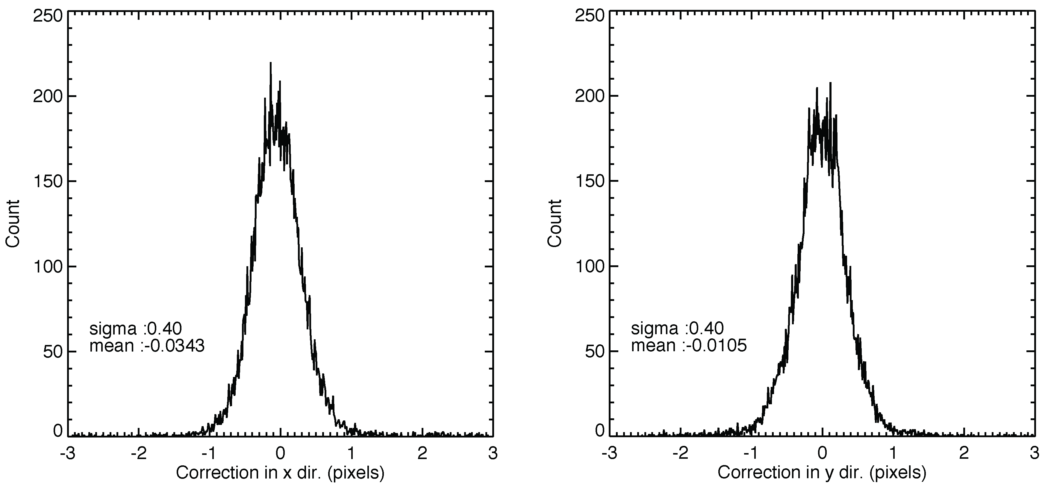
With this scheme, large regions with variable surface velocity and no low/zero-motion areas may require additional calibration because a change in speed between the reference map and the actual scene may bias the calibration. Such regions include Thwaites Glacier in West Antarctica or Larsen C Ice Shelf in the Antarctic Peninsula for example. Our solution for these areas is to concatenate the Sentinel-1 scenes into long tracks where areas of low motion are found systematically and we then use these long tracks to calibrate shorter Landsat-8 or Sentinel-1a scenes. In principle, the Landsat-8 offset maps require no additional calibration if the images are accurately geocoded. Thus, the distribution of correction we apply to the data is directly linked to the quality of the geocoding (Figure 1). We find that Landsat images are georeferenced with a precision of 0.0 ± 0.4 pixel, or 0.2 ± 6.0 m in both x- and y-direction, which is consistent with the geolocation accuracy derived by [28]. If not properly corrected, a geocoding error of 0.4 pixel would introduce an error in velocity measurement ranging from 137 m/year for 16-day to 5 m/year for 368-day passes.
Data products are geocoded in Polar Stereographic coordinates. For Sentinel-1, the geocoding uses the GIMP digital elevation model of Greenland [29] and the BEDMAP-2 digital elevation model of Antarctica [30]. Errors on the offset maps are assumed to be 0.1 pixel in displacement by default. Typically, the errors in ice velocity are then a few tens of meters per year for the nominal repeat cycle of the sensors (see Table 1). The precision of a sensor depends on the resolution and the repeat cycle. Because sensors differ in both, their precision varies accordingly. Table 1 provides a reference only, not for the purpose of comparing the different sensors.
2.5. Annual Ice Velocity Mosaics
Yearly mosaics are formed with all acquisitions spanning from 1 July to 30 June of the next year (centered on 1 January). We use this convention because previous SAR campaigns (2000–2010) from ALOS/PALSAR, ENVISAT/ASAR or RADARSAT-1&-2 were mostly acquired between October and March. Here, we focus on the mosaics generated for years 2013–2014, 2014–2015 and 2015–2016. These yearly mosaics are generated in 3 steps as follows:
- If the number of acquisitions (per pixel) is greater than two, we compute the median and the standard deviation for each pixel individually over all the acquisitions made during the year.
- We remove measurements that exceed from the median:
- We then compute the weighted mean, weighted standard error, weighted standard deviation on remaining values. The weights are taken as , where are the precision in ice velocity as listed in Table 1.
3. Results
3.1. Antarctica
3.1.1. Landsat-8
We process 26192, 61223 and 24169 pairs of Landsat-8 images for years 2013–2014, 2014–2015 and 2015–2016, respectively. We assemble them in annual mosaics of surface ice velocity (see Figure 2a–c) following the approach described previously. The 2013–2014 mosaic (Figure 2a) is the least complete in the interior because fewer acquisitions were made compared to later years, but it includes a complete coverage of the coastal regions. For years 2014–2015 and 2015–2016 (Figure 2b,c), a large numbers of acquisitions were made in the interior, resulting in a more complete and dense coverage up to 82.7S. Most of the regions north of 82.7S are covered by more than 100 correlating pairs. Regions where correlation is lower are the west side of the Antarctic Peninsula, Walgreen Coast, Getz Coast, and Eltanin Bay in West Antarctica. These regions are characterized by high accumulation of snowfall and high surface weathering [21,31], which alter the surface features needed for image correlation. Errors in ice surface velocity may exceed 20 m/year along the coast of Antarctica (see Figure 2), where the image pairs use the shortest repeat cycles, hence the largest errors, and surface weathering (accumulation, wind and/or melt) is most significant. The interior is mapped using a combination of pairs with repeat pass larger than 64 days, leading to standard deviations at a few meters per year level.
3.1.2. RADARSAT-2 & Sentinel-1a
Concurrently with the Landsat-8 mosaic, RADARSAT-2 in 2013–2014 and Sentinel-1a in 2014–2015 and 2015–2016, provide annual mosaics with a C-band radar sensors (Figure 2d–f). For year 2013–2014, RADARSAT-2 (Figure 2d) completed a large coastal mapping with up to 5 pairs per survey point. As expected from earlier mappings with ENVISAT ASAR, West Antarctica and the Antarctic Peninsula are regions that display low correlation due to the relatively long revisit period combined with surface weathering. Each year, RADARSAT-2 is the only sensor that provides a partial view of the Antarctic interior. With all years merged together (2013 to 2016), the RADARSAT-2 coverage offers a comprehensive view south of 78S latitude. In 2014–2015, Sentinel-1a started acquiring data over Antarctica. The resulting mosaic (Figure 2e) from the 1448 pairs of scenes shows relatively good correlation where data were acquired in the western sectors of Antarctica. In 2015–2016, good coverage of all of Antarctica (south of 78.65S, or 4 degrees less than Landsat-8) was achieved with Sentinel-1a (Figure 2f) and a total of 3461 pairs were processed. Overlap between acquisitions is slightly higher with the 2015 Sentinel-1a, with 5 to 10 overlapping pairs, than with RADARSAT-2 in 2013. Most of the mapped regions are covered with less than 5 pairs. The regions presenting low correlation are the same as in the case of Landsat with the addition of Wilkes Land, East Antarctica, known for strong katabatic winds. Standard deviations for the different mosaics are between 10 and 20 m/year.
3.2. Greenland
3.2.1. Landsat-8
In Greenland, we processed 3783, 13063 and 9257 Landsat pairs for years 2013–2014, 2014–2015, 2015–2016 and assembled the mosaics shown in Figure 3a–c. Correlation increases with latitude, allowing a more complete mapping of the northern part of Greenland. Surface features in the interior of the ice sheets seem to be less persistent than in Antarctica, thus strong decorrelation occurs for 64 days repeat cycle. As a result, the standard deviations are larger than those estimated in interior Antarctica, typically 10 to 20 m/year.
3.2.2. RADARSAT-2 & Sentinel-1a
In year 2013-2014, RADARSAT-2 provided a partial coverage of Greenland (Figure 3d), mainly limited by mode conflicts with interests from the Canadian government and commercial companies. Comprehensive mappings from Sentinel-1a for years 2014–2015 and 2015–2016 have been obtained from 677 and 2982 scenes (Figure 3e,f). The mapping coverage is similar to the 2014–2015 comprehensive map done by [19] and to its Landsat counterpart. Overall, previous mappings with C-band sensors, such as RADARSAT-1 (24 days repeat, [1,3] or ENVISAT/ASAR (35 days repeat, [3]), displayed less correlation than Sentinel-1a/b, especially in the southern part of Greenland. This suggests that the shorter repeat cycle of Sentinel-1a/b, in addition to continuous mapping, is significantly useful to improve ice sheet mapping.
3.3. Comparison of Ice Velocity Products
3.3.1. Individual Measurements
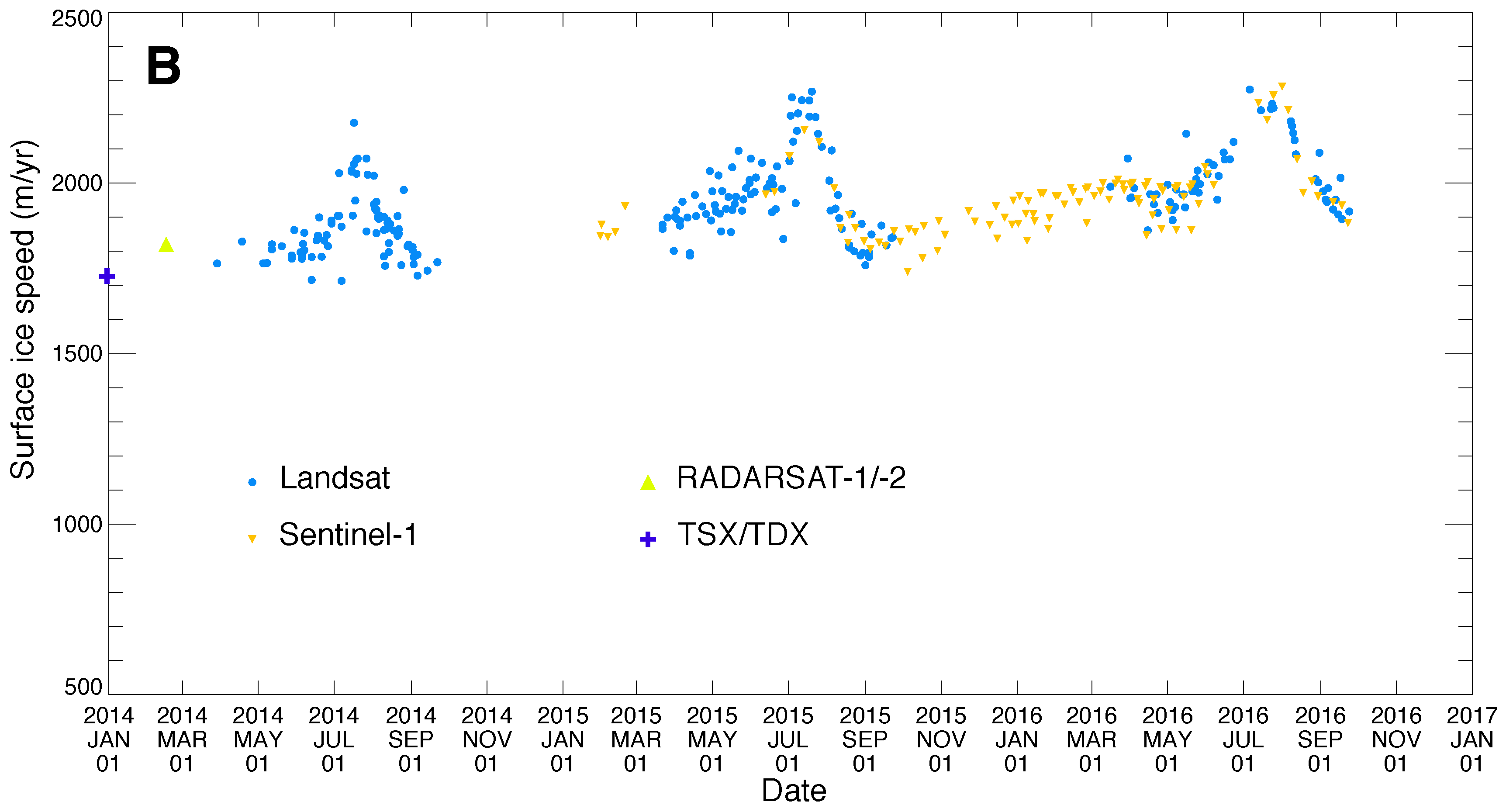
The large number of acquisitions allows the formation of dense time series to observe temporal variations in ice velocity over shorter periods. We compare results from offset maps (without mosaicking) in a time series of Zachariae Isstrøm, in Northeast Greenland. Figure 4 shows the evolution of ice speed of Zachariae near its 2015 grounding line using historical data [34], Landsat-8 (blue dots) and Sentinel-1 (orange triangles). The two datasets, Sentinel-1 and Landsat-8, are consistent with each other and with measurements from preceding years based on TerraSAR-X and RADARSAT-2. The number of measurement points increased significantly with Landsat-8 and Sentinel-1. Landsat-8 is only acquired in summer and is complemented by Sentinel-1a year round. In the case of Zachariae Isstrøm, we observe that the glacier did not exhibit seasonal velocity variations until about year 2005 when we detect significant seasonal variations, up to 20%, which increase till present. We attribute this behavior to the progressive disappearance of its floating ice shelf and to the increase in calving events and subsurface melting by the ocean of its ice front [34]. A similar behavior was observed on Jakobshavn Isbræ after its ice shelf broke off in year 2002 whereas no seasonal variation was detected on this glacier in the past [35,36].
3.3.2. Mean Area-Percentage of Spatial Coverage Per Scene
In order to compare the ability to map ice speed over large regions with Landsat-8 and Sentinel-1, we compute the area-percentage of spatial coverage per scene where ice velocity is successfully tracked over Antarctica excluding the ocean. With the 29,838 Landsat-8 16-day image pairs processed, we find that on average 33% of the scene area is usable for ice speed mapping. As we only used image pairs with less than 80% cloud coverage, this estimate is even lower for the entire archive, i.e., if we include images with 100% cloud coverage. The main limiting factor for spatial coverage with Landsat is cloud cover. Indeed, we find that the mean area-percentage of spatial coverage per scene in the interior of East Antarctica for images with less than 10% cloud cover is 77, 72 and 61% for 64, 80 and 368 days repeat, respectively. This high correlation rate, even from 1 year pairs, indicates that surface features needed for the image correlation are stable over long periods of time in some regions. Sentinel-1 with 12-day pairs has a comparable success rate with a mean area-percentage of 42.2% for the 4057 scenes processed in Antarctica. For Sentinel-1, the decorrelation occurs mostly in regions with low radar backscatter, which correspond to regions with high accumulation of snowfall [38].
3.3.3. Ice Velocity Precision
To assess the precision of the velocity products using independent observations, we form individual mosaics for each of the processed cycles and each sensor including historic data, such as ENVISAT ASAR, ALOS/PALSAR, as well as RADARSAT-2 data from 2009–2011 (Figure 5). We use the standard deviation derived for each pixel of the mosaics as an estimation of the precision of one ice velocity measurement. Figure 6a shows the distributions of this standard deviation for each mosaic made from a specific sensor and repeat cycle. To be statistically significant, we only keep pixels with more than 10 measurements and for which the absolute speed is less than 300 m/year (to minimize to the influence of ice flow changes). We find that the most probable standard deviation for the Landsat mosaics using the 16, 32, 48, 64, 80 and 368-day cycles are respectively 17, 11, 7, 6, 5 and 1 m/year, which provides a direct estimation of the precision of the ice velocity measurement for an individual scene. By converting this precision in ice displacement (m/year) into offset (pixel), we find that precision of the image correlation ranges between 0.05 and 0.07 pixels, or twice lower than the default precision in Table 1.
The same estimations for the C-Band SAR sensors reveal that the nominal standard deviation is lower for similar repeat cycles (Figure 6b). Sentinel-1 with 6, 12 and 24-day cycles, RADARSAT-2 with 24-day cycle, and ENVISAT/ASAR with 35-day cycle, have standard deviations in the range of 17, 8, 5, 4 and 3 m/year, respectively. It is difficult to assess exactly the corresponding error of image cross-correlation as the native pixel of the SAR observations are not square, but we estimate this value to be between 0.02 and 0.05 pixel depending on the range or azimuth resolution chosen (see Table 1).
The slightly more precise cross-correlation results from C-Band SARs may be attributed to the better spatial resolution of the raw data. It is also possible that the tracking of image speckle in SAR data is more efficient than surface features in Landsat-8 data because of the availability of amplitude and phase that allow more precise image interpolation.
3.3.4. Mosaic Difference
To assess the difference between Sentinel-1a/b and Landsat-8 velocity results, we compare Antarctica mosaics for year 2015–2016 produced from each sensor (Figure 7). We find that the mean differences (Sentinel-1 minus Landsat-8) for the speed in x- and y- directions are −0.7 and −0.3 m/year, with a standard deviation of 18.9 and 18.0 m/year, respectively. These values are consistent with the standard deviation maps for the annual mosaics produced in Figure 2. Overall we conclude that the results from both sensors are in excellent agreement. Absolute differences in the interior are generally less than 10 m/year, but can be locally larger because of the ionosphere streaking [39] or low correlation in Sentinel-1a/b. Along the coast, larger differences (<50 m/year) are found, which are caused by stronger weathering, ionospheric noise, and ongoing velocity changes.
We also compare our mosaics (Figure 3) with the ENVEO’s (http://www.enveo.at/) ice velocity mosaic products of Greenland published by [19] for year 2014–2015 and 2015–2016 from Sentinel-1 acquisitions. We find that the ENVEO’s velocity maps are in good agreement with our Landsat-8 and Sentinel-1 mosaics. The distribution of the difference between the absolute ice speed from ENVEO minus the results from this study is shown in Figure 8. Typically, the mean differences between ENVEO and this study for year 2015–2016 are 0 ± 11 and 0 ± 7 m/year for Sentinel-1 and Landsat-8, respectively.
4. Discussion
4.1. Potential of Landsat-8 for Large Scale Ice Velocity Mapping Compared with Current SAR Missions
Since 2013, RADARSAT-2, Sentinel-1a and Landsat-8 have acquired large datasets over Greenland and Antarctica. We have processed both types of data sets and generated comparable maps of ice motion. The comparison of radar and optical ice velocity maps show that (i) the individual ice velocity measurements are equivalentbetween Landsat-8 and Sentinel-1; (ii) the precision is comparable for identical repeat cycle; (iii) area-coverage per scene where ice speed is mapped is roughly equivalent; and (iv) the annual mosaic products are similar within the error associated with both sensors.
As in the case of radar sensors, optical sensors have limitations. We note that a calibration of the Landsat-8 offsets is necessary to ensure accurate ice velocity measurement (Figure 1). Small inaccuracy in the geolocation of the Landsat-8 (±6 m) images [28] can generate errors in speed up to 137 m/year for 16-day cycle. As the geolocation improves, this problem might be alleviated, especially if more accurate DEMs of Greenland and Antarctica become available and are used for geocoding. In that regard, it would be important to archive the level 0 image data, i.e., without geocoding, so the image geolocation and ortho-rectification can be improved in the future.
Solar illumination is another limitation for optical data compared to SAR data. Figure 5b shows that, in polar regions, acquisitions limited to the summer season make it impossible to track the entire seasonal cycle in speed of Greenland glaciers. In Antarctica, we find that the mean correlation for a single Landsat scene is about 33%, mostly due to cloud cover, whereas SAR shows a correlation of 42%. We note that SAR decorrelation is often located in the same geographic region, i.e., caused by surface climate, whereas Landsat-8 decorrelation is mostly due to clouds and hence varies spatially. Given the same revisit time, SAR C-band velocity tracking is more precise than optical (Figure 7).
One advantage of Landsat-8 comes from the large amount data acquired during the past years. It is reasonable to expect that SAR sensors would provide comparable if not superior quality data with the same rate of acquisition. It was also surprising to find out that Landsat-8 correlates even with 1-year time separation [21]. We have less experience doing this with SAR because it requires a good orbit control (small baselines) [40] over a long time and most SAR sensors have not tried to do so, but given proper baseline control the same success could be achieved with SAR sensors.
These results demonstrate that the quality of the products generated from optical satellite sensors is comparable to that obtained with SAR sensors (Figure 2, Figure 3 and Figure 4). Cloud cover that limits spatial coverage with optical sensors is no longer a limiting factor for annual mapping due to the dense temporal coverage. In addition, optical images are simpler and faster to process.
4.2. Integration of Multi-Sensor Data
Having seamless and comprehensive continental-wide maps of ice velocity is crucial for the scientific community to study the evolution of ice sheets in a warmer climate, but his task remains technically challenging especially when trying to make annual time series [1,3,19,41]. This is the main reason why we have, so far, to rely on different sensors in order to obtain a comprehensive view of the dynamics of the ice sheets. Thus each sensor contributes uniquely to the final map [22]. The different advantages range from spatial coverage (e.g., South Pole covered by RADARSAT-2 only) to better correlation (L-band). In this way, the integration of Landsat-8 to the SAR sensors used previously [22] allows to provide a more complete coverage of the ice velocity in Greenland and Antarctica than achieved with single sensor. Indeed, combining the new datasets, RADARSAT-2, Sentinel-1 and Landsat-8, with the previous sensors (ERS, ENVISAT/ASAR, ALOS/PALSAR, RADARSAT-1) we cover 99.6% and 99.9% of the Antarctic (Figure 9) and Greenland (Figure 10) ice sheets, respectively versus our earlier mappings [2,3] that covered 95.1% and 97.4%. These complete products will benefit glaciologists and ice sheet modelers by providing maps with no gap, continuous data, and improved precision.
4.3. Implications for (Future) SAR Missions for Ice Velocity Measurements
Landsat-8 demonstrated great capabilities for ice velocity mapping over ice sheets and the vast amount of data acquired by USGS greatly enhances its utility. There continues to be downsides to optical data, which justifies the continued use of spaceborne SAR data. These downsides include (i) a lack of illumination for part of the year; (ii) cloud cover (which is frequent in some areas); and (iii) lower precision of optical (assuming the same amount of data).
We note that all ice motion measurements being discussed here use feature tracking (Landsat-8) or speckle tracking (SAR). This technique is limited by the size of the pixel element (or resolution cell of the data) and data noise. With SAR sensors, however, it is possible to measure ice motion with the interferometric phase instead [12,17,42,43,44,45]. The precision of ice motion from the phase is not limited by the pixel size, but by the size of the radar wavelength and data noise. In effect, SAR sensors measure ice motion within millimeters using the phase, or typically one order magnitude better than with tracking [46]. In that case, given the same amount of data and the same pixel size, SAR sensors offer vastly superior quality for ice motion measurements. On the other hand, phase measurements need to be completed along two independent directions (or three if we do not assume surface parallel flow [14]) in order to resolve the vector of ice motion, hence require more data acquisition and tracks [47]. With the interferometric phase, SAR sensors also detect differential movements of the ice surface, e.g., the subtle flapping of floating sections up and down with changes in oceanic tides [41,48], or the deflation of the ice surface because of drainage of a subglacial lake, at a precision of a few millimeters, which is currently impossible to achieve from optical sensors or altimeters and is a unique capability of SAR sensors. The use of phase data however require twice more data compared to the correlation technique ascending and descending acquisitions are needed. The current SAR sensors (Sentinel-1, RADARSAT-2, TSX) are not ideal for using the phase on a large scale because of their limited coverage and/or their operational mode of acquisition which is not optimum for phase analysis.
In the future, the upcoming SAR missions from the CSA’s RADARSAT Constellation Mission (RCM) or the NASA/ISRO InSAR mission (NISAR) will provide new opportunities to use phase mapping. NASA and ISRO will launch NISAR (https://nisar.jpl.nasa.gov/) in 2020 to completely and continuously survey the ice sheets on a 12-day cycle at the L-band frequency for a nominal mission time of three years [49]. From the archive of ALOS/PALSAR already processed [2,22,50], we know that L-band SAR with a cycle of 46 days achieves successful velocity mapping on an area-percentage per scene of 73% in Antarctica. We reasonably expect a higher correlation level for a repeat cycle 4 times shorter. In addition, NISAR will enable phase measurements pole to pole, hence more precise measurements of ice motion, day and night, summer or winter. Along the coastal areas, where ice motion is too large to track with the interferometric phase, we will continue to employ the speckle tracking technique and it is likely that the addition of Landsat-8 data will remain a significant source of additional information on ice motion. Similarly, Sentinel-1a/b has opened new opportunities for mapping ice motion in the polar regions. Since both the Landsat and Sentinel are planned to be long term programs, these assets will remain at the service of the scientific community for decades to come.
5. Conclusions
In this study, we employed large quantities of Landsat-8 and Sentinel-1a/b data to map ice motion pole-to-pole in Greenland and Antarctica. We compared and contrasted data quality between these sensors at retrieving ice motion. We implemented a system which processes the data automatically, calibrates them automatically given prior maps of ice motion, and which mosaics them automatically. We combined the results from image pairs with different time separation and hence difference noise levels, weighting the results with data noise, to create merged products from SAR and optical sensors that cover the entire ice sheets on an annual basis. We have demonstrated that the quality of the Landsat-8 data is now comparable to that achievable with SARs so that the merging of data products (spatially as well as for time series) is not only possible but desirable. We expect the resulting output products of ice motion to be of considerable interest to study glacier dynamics, ice discharge, the contribution of glaciers and ice sheets to sea level rise, and to improve numerical models used to project the evolution of these ice sheets in a warmer climate.
Acknowledgments
We thank the space agencies (NASA, ESA, CSA, JAXA, ASI, DLR) which made this work possible by making satellite observations of the polar regions free access to our research group and the entire scientific community. We also thank the PSTG for coordinating data acquisitions in the polar regions since the 2007–2008 International Polar Year. This work was performed at UC Irvine and at Caltech’s Jet Propulsion Laboratory under contracts with the Cryosphere Program and the MEASURES Program of the National Aeronautics and Space Administration (NASA). Annual velocity maps as well as the integrated multi sensor velocity map will be made available at NSIDC (http://nsidc.org/data/measures).
Author Contributions
Jeremie Mouginot, Bernd Scheuchl and Eric Rignot wrote the paper and supervised the project. Jeremie Mouginot and Bernd Scheuchl processed the data. Jeremie Mouginot, Bernd Scheuchl and Romain Millan designed the processing chain. All authors discussed the results and commented on the manuscript at all stages.
Conflicts of Interest
The authors declare no conflict of interest.
References
- Joughin, I.; Smith, B.; Howat, I.; Scambos, T.; Moon, T. Greenland flow variability from ice-sheet-wide velocity mapping. J. Glaciol. 2010, 56, 416–430. [Google Scholar] [CrossRef]
- Rignot, E.; Mouginot, J.; Scheuchl, B. Ice Flow of the Antarctic Ice Sheet. Science 2011, 333, 1427–1430. [Google Scholar] [CrossRef] [PubMed]
- Rignot, E.; Mouginot, J. Ice flow in Greenland for the International Polar Year 2008-2009. Geophys. Res. Lett. 2012, 39, L11501. [Google Scholar] [CrossRef]
- Rignot, E.; Kanagaratnam, P. Changes in the velocity structure of the Greenland ice sheet. Science 2006, 311, 986–990. [Google Scholar] [CrossRef] [PubMed]
- Rignot, E.; Bamber, J.; van den Broeke, M.; Davis, C.; Li, Y.; van de Berg, W.; van Meijgaard, E. Recent Antarctic ice mass loss from radar interferometry and regional climate modelling. Nature Geosci. 2008, 1, 106–110. [Google Scholar] [CrossRef]
- Enderlin, E.M.; Howat, I.M.; Jeong, S.; Noh, M.J.; van Angelen, J.H.; van den Broeke, M.R. An improved mass budget for the Greenland ice sheet. Geophys. Res. Lett. 2014, 41, 866–872. [Google Scholar] [CrossRef]
- Lucchitta, B.K.; Ferguson, H.M. Antarctica: Measuring Glacier Velocity from Satellite Images. Science 1986, 234, 1105–1108. [Google Scholar] [CrossRef] [PubMed]
- Bindschadler, R.A.; Scambos, T.A. Satellite-Image-Derived Velocity Field of an Antarctic Ice Stream. Science 1991, 252, 242–246. [Google Scholar] [CrossRef] [PubMed]
- Scambos, T.A.; Bohlander, J.A.; Shuman, C.A.; Skvarca, P. Glacier acceleration and thinning after ice shelf collapse in the Larsen B embayment, Antarctica. Geophys. Res. Lett. 2004, 31, L18402. [Google Scholar] [CrossRef]
- Rosenau, R.; Scheinert, M.; Dietrich, R. A processing system to monitor Greenland outlet glacier velocity variations at decadal and seasonal time scales utilizing the Landsat imagery. Remote Sens. Environ. 2015, 169, 1–19. [Google Scholar] [CrossRef]
- Goldstein, R.M.; Engelhardt, H.; Kamb, B.; Frolich, R.M. Satellite Radar Interferometry for Monitoring Ice Sheet Motion: Application to an Antarctic Ice Stream. Science 1993, 262, 1525–1530. [Google Scholar] [CrossRef] [PubMed]
- Rignot, E.; Jezek, E.; Sohn, H. Ice Flow Dynamics of the Greenland Ice Sheet from SAR Interferometry. Geophys. Res. Lett. 1995, 2, 575–578. [Google Scholar] [CrossRef]
- Michel, R.; Rignot, E. Flow of Glaciar Moreno, Argentina, from repeat-pass Shuttle Imaging Radar images: comparison of the phase correlation method with radar interferometry. J. Glaciol. 1999, 45, 93–100. [Google Scholar] [CrossRef]
- Joughin, I.R.; Kwok, R.; Fahnestock, M.A. Interferometric estimation of three-dimensional ice-flow using ascending and descending passes. IEEE Trans. Geosci. Remote Sens. 1998, 36, 25–37. [Google Scholar] [CrossRef]
- Jezek, K.C.; Sohn, H.; Noltimier, K. The RADARSAT Antarctic mapping project. IEEE Int. Geosci. Remote Sens. Symp. 1998, 5, 2462–2464. [Google Scholar]
- Gray, A.; Mattar, K.; Vachon, P.; Bindschadler, R.; Jezek, K.; Forster, R.; Crawford, J. InSAR results from the RADARSAT Antarctic Mapping Mission data: Estimation of glacier motion using a simple registration procedure. IEEE Int. Geosci. Remote Sens. Symp. 1998, 3, 1638–1640. [Google Scholar]
- Joughin, I.R.; Winebrenner, D.P.; Fahnestock, M.A. Observations of ice-sheet motion in Greenland using satellite radar interferometry. Geophys. Res. Lett. 1995, 22, 571–574. [Google Scholar] [CrossRef]
- Joughin, I. Ice-sheet velocity mapping: A combined interferometric and speckle-tracking approach. Ann. Glaciol. 2002, 34, 195–201. [Google Scholar] [CrossRef]
- Nagler, T.; Rott, H.; Hetzenecker, M.; Wuite, J.; Potin, P. The Sentinel-1 Mission: New Opportunities for Ice Sheet Observations. Remote Sens. 2015, 7, 9371–9389. [Google Scholar] [CrossRef]
- Jeong, S.; Howat, I.M. Performance of Landsat 8 Operational Land Imager for mapping ice sheet velocity. Remote Sens. Environ. 2015, 170, 90–101. [Google Scholar] [CrossRef]
- Fahnestock, M.; Scambos, T.; Moon, T.; Gardner, A.; Haran, T.; Klinger, M. Rapid large-area mapping of ice flow using Landsat 8. Remote Sens. Environ. 2016, 185, 84–94. [Google Scholar] [CrossRef]
- Mouginot, J.; Scheuchl, B.; Rignot, E. Mapping of Ice Motion in Antarctica Using Synthetic-Aperture Radar Data. Remote Sens. 2012, 4, 2753–2767. [Google Scholar] [CrossRef]
- Dehecq, A.; Gourmelen, N.; Emmanuel, T. Deriving large-scale glacier velocities from a complete satellite archive: Application to the Pamir–Karakoram–Himalaya. Remote Sens. Environ. 2015, 162, 55–66. [Google Scholar] [CrossRef]
- Rosen, P.A.; Hensley, S.; Peltzer, G.; Simons, M. Updated repeat orbit interferometry package released. Eos Trans. Amer. Geophys. Unio 2004, 85, 47. [Google Scholar] [CrossRef]
- Meta, A.; Mittermayer, J.; Prats, P.; Scheiber, R.; Steinbrecher, U. TOPS imaging with TerraSAR-X: Mode design and performance analysis. IEEE Trans. Geosci. Remote Sens. 2010, 48, 759–769. [Google Scholar] [CrossRef]
- Scheuchl, B.; Mouginot, J.; Rignot, E.; Morlighem, M.; Khazendar, A. Grounding line retreat of Pope, Smith, and Kohler Glaciers, West Antarctica, measured with Sentinel-1a radar interferometry data. Geophys. Res. Lett. 2016, 43, 8572–8579. [Google Scholar] [CrossRef]
- Scheuchl, B.; Mouginot, J.; Rignot, E. Ice velocity changes in the Ross and Ronne sectors observed using satellite radar data from 1997 and 2009. The Cryosphere 2012, 6, 1019–1030. [Google Scholar] [CrossRef]
- Storey, J.; Choate, M.; Lee, K. Landsat 8 Operational Land Imager On-Orbit Geometric Calibration and Performance. Remote Sens. 2014, 6, 11127–11152. [Google Scholar] [CrossRef]
- Howat, I.M.; Negrete, A.; Smith, B.E. The Greenland Ice Mapping Project (GIMP) land classification and surface elevation data sets. Cryosphere 2014, 8, 1509–1518. [Google Scholar] [CrossRef]
- Fretwell, P.; Pritchard, H.D.; Vaughan, D.G.; Bamber, J.L.; Barrand, N.E.; Bell, R.; Bianchi, C.; Bingham, R.G.; Blankenship, D.D.; Casassa, G.; et al. Bedmap2: Improved ice bed, surface and thickness datasets for Antarctica. Cryosphere 2013, 7, 375–393. [Google Scholar] [CrossRef]
- Van Wessem, J.; Reijmer, C.; Morlighem, M.; Mouginot, J.; Rignot, E.; Medley, B.; Joughin, I.; Wouters, B.; Depoorter, M.; Bamber, J.; Lenaerts, J.; De Van Berg, W.; Van Den Broeke, M.; Van Meijgaard, E. Improved representation of East Antarctic surface mass balance in a regional atmospheric climate model. J. Glaciol. 2014, 60, 761–770. [Google Scholar] [CrossRef]
- Scambos, T.; Haran, T.; Fahnestock, M.; Painter, T.; Bohlander, J. MODIS-based Mosaic of Antarctica (MOA) data sets: Continent-wide surface morphology and snow grain size. Remote Sens. Environ. 2007, 111, 242–257. [Google Scholar] [CrossRef]
- Haran, T.; Bohlander, J.; Scambos, T.; Painter, T.; Fahnestock, M. MODIS Mosaic of Greenland (MOG) Image Map; NSIDC: National Snow and Ice Data Center: Boulder, CO, USA, 2013. [Google Scholar]
- Mouginot, J.; Rignot, E.; Scheuchl, B.; Fenty, I.; Khazendar, A.; Morlighem, M.; Buzzi, A.; Paden, J. Fast retreat of Zachariae Isstrom, northeast Greenland. Science 2015, 350, 1357–1361. [Google Scholar] [CrossRef] [PubMed]
- Luckman, A.; Murray, T. Seasonal variation in velocity before retreat of Jakobshavn Isbræ, Greenland. Geophys. Res. Lett. 2005, 32, L08501. [Google Scholar] [CrossRef]
- Joughin, I.; Smith, B.E.; Shean, D.E.; Floricioiu, D. Brief Communication: Further summer speedup of Jakobshavn Isbræ. Cryosphere 2014, 8, 209–214. [Google Scholar] [CrossRef]
- Ahn, Y.; Howat, I.M. Efficient Automated Glacier Surface Velocity Measurement From Repeat Images Using Multi-Image/Multichip and Null Exclusion Feature Tracking. IEEE Trans. Geosci. Remote Sens. 2011, 49, 2838–2846. [Google Scholar]
- Hoen, E.W.; Zebker, H.A. Penetration depths inferred from interferometric volume decorrelation observed over the Greenland Ice Sheet. IEEE Trans. Geosci. Remote Sens. 2000, 38, 2571–2583. [Google Scholar]
- Gray, A.L.; Mattar, K.E.; Sofko, G. Influence of ionospheric electron density fluctuations on satellite radar interferometry. Geophys. Res. Lett. 2000, 27, 1451–1454. [Google Scholar] [CrossRef]
- Rosen, P.A.; Hensley, S.; Joughin, I.R.; Li, F.K.; Madsen, S.N.; Rodriguez, E.; Goldstein, R.M. Synthetic aperture radar interferometry. IEEE Proc. 2000, 88, 333–382. [Google Scholar] [CrossRef]
- Rignot, E.; Mouginot, J.; Scheuchl, B. Antarctic grounding line mapping from differential satellite radar interferometry. Geophys. Res. Lett. 2011, 38, 1–6. [Google Scholar] [CrossRef]
- Kwok, R.; Fahnestock, M.A. Ice sheet motion and topography from radar interferometry. IEEE Trans. Geosci. Remote Sens. 1996, 34, 189–200. [Google Scholar] [CrossRef]
- Mohr, J.J.; Reeh, N.; Madsen, S.N. Three-dimensional glacial flow and surface elevation measured with radar interferometry. Nature 1998, 391, 273–276. [Google Scholar]
- Rignot, E.; Gogineni, S.P.; Krabill, W.B.; Ekholm, S. North and northeast Greenland ice discharge from satellite radar interferometry. Science 1997, 276, 934–937. [Google Scholar] [CrossRef]
- Goldstein, R.M.; Werner, C.L. Radar interferogram filtering for geophysical applications. Geophys. Res. Lett. 1998, 25, 4035–4038. [Google Scholar] [CrossRef]
- Rott, H. Advances in interferometric synthetic aperture radar (InSAR) in earth system science. Progr. Phys. Geogr. 2009, 33, 769–791. [Google Scholar] [CrossRef]
- Gray, L. Using multiple RADARSAT InSAR pairs to estimate a full three-dimensional solution for glacial ice movement. Geophys. Res. Lett. 2011, 38, L05502. [Google Scholar] [CrossRef]
- Rignot, E. Tidal motion, ice velocity and melt rate of Petermann Gletscher, Greenland, measured from radar interferometry. J. Glaciol. 1996, 42, 476–485. [Google Scholar] [CrossRef]
- Rosen, P.; Hensley, S.; Shaffer, S.; Edelstein, W.; Kim, Y.; Kumar, R.; Misra, T.; Bhan, R.; Satish, R.; Sagi, R. An update on the NASA-ISRO dual-frequency DBF SAR (NISAR) mission. IEEE Int. Geosci. Remote Sens. Symp. 2016. [Google Scholar] [CrossRef]
- Rignot, E. Changes in West Antarctic ice stream dynamics observed with ALOS PALSAR data. Geophys. Res. Lett. 2008, 35, 1–5. [Google Scholar] [CrossRef]
Figure 1.
Distribution of the calibration constants applied to Landsat-8 data along the x (easting) and y (northing) direction (in polar stereographic projection).
Figure 1.
Distribution of the calibration constants applied to Landsat-8 data along the x (easting) and y (northing) direction (in polar stereographic projection).

Figure 2.
Annual mosaics of surface ice speed generated from Landsat-8 (A–C) and the SAR sensors Sentinel-1 and RADARSAT-2 (D–F) in Antarctica. The figure is constructed as a matrix, the 3 rows representing the different years surveyed (2013, 2014, 2015) and the 2 columns representing the different sensors (optical and SAR). The ice velocity is coded on a logarithmic scale overlaid on MOA background mosaic [32]. Each velocity map is accompanied by 3 additional panels representing the number of velocity measurements (top), the weighted standard deviation in x- (middle) and y-direction (bottom). Standard deviations are calculated when 3 or more velocity measurements are present and replaced by the weighted standard error when less than 3 measurements are found.
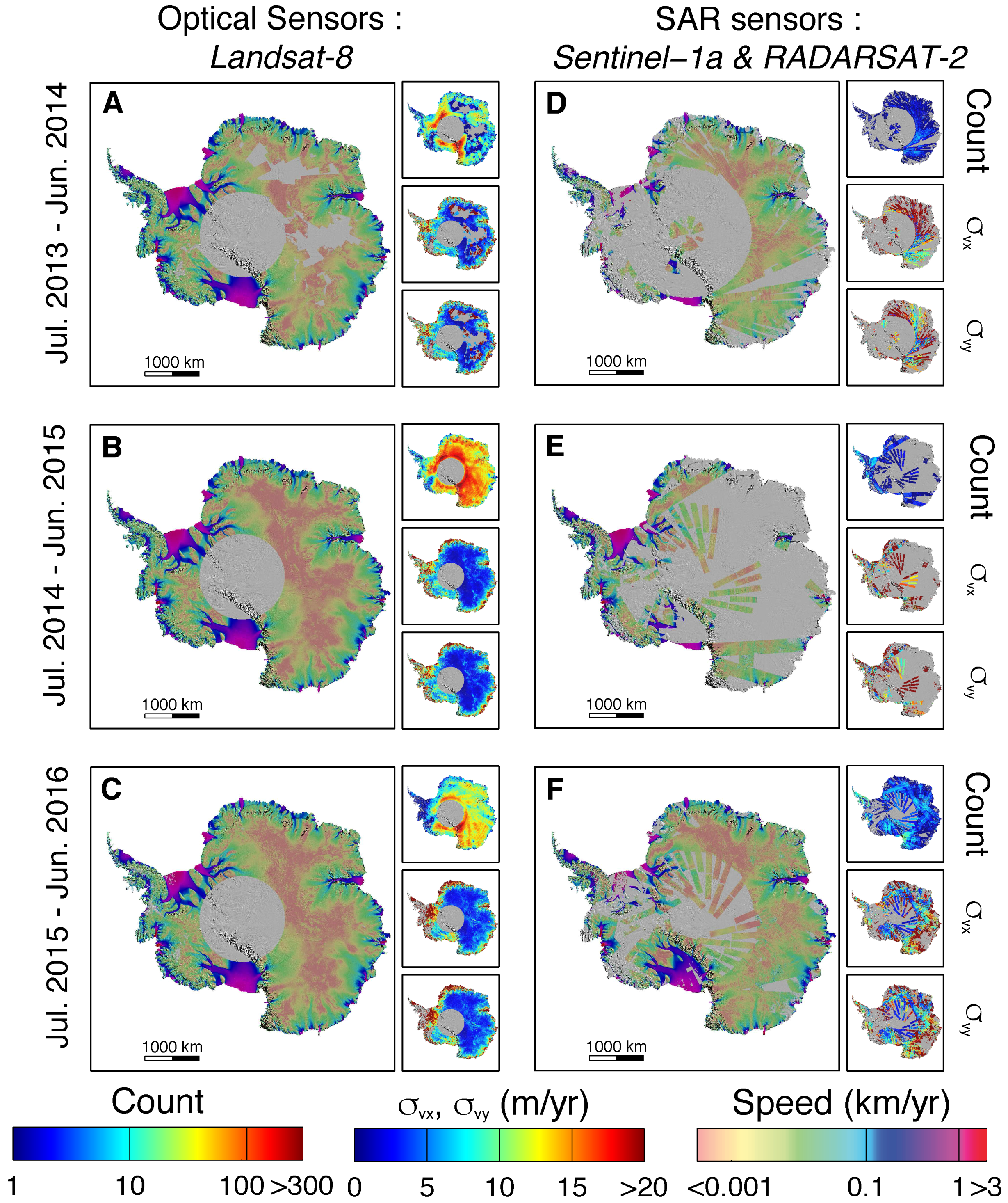
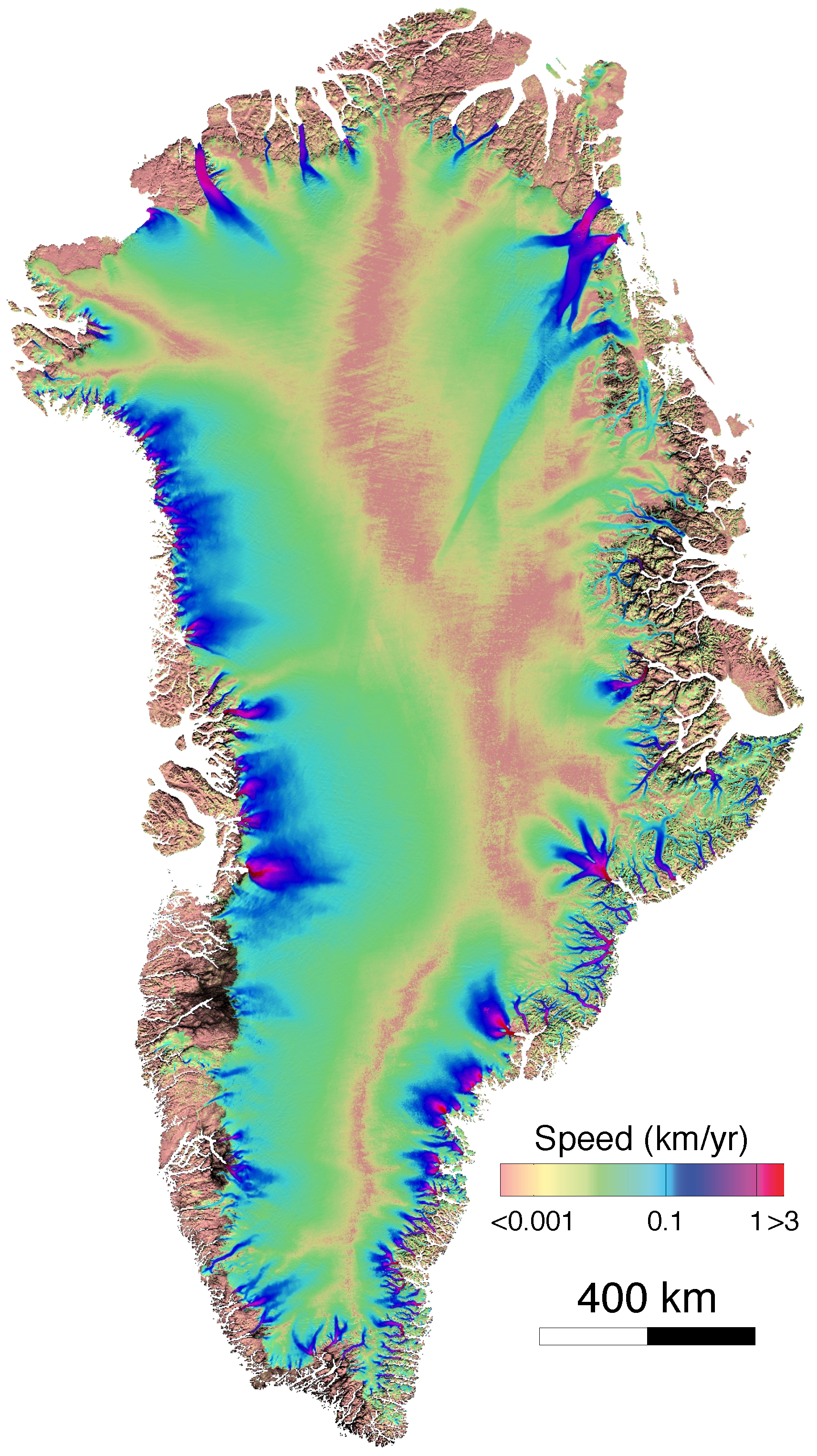
Figure 3.
Annual mosaics of surface ice speed generated from Landsat-8 (A–C) and the SAR sensors Sentinel-1 and RADARSAT-2 (D–F) in Greenland. The figure is constructed as a matrix, the 3 rows representing the different years surveyed (2013, 2014, 2015) and the 2 columns representing the different sensors (optical and SAR). The ice velocity is coded on a logarithmic scale overlaid on MOG background mosaic [33]. Each velocity map is accompanied by 3 additional panels representing the number of velocity measurements (top), the weighted standard deviation in x- (middle) and y-direction (bottom). Standard deviations are calculated when 3 or more velocity measurements are present and replaced by the weighted standard error when less than 3 measurements are found.
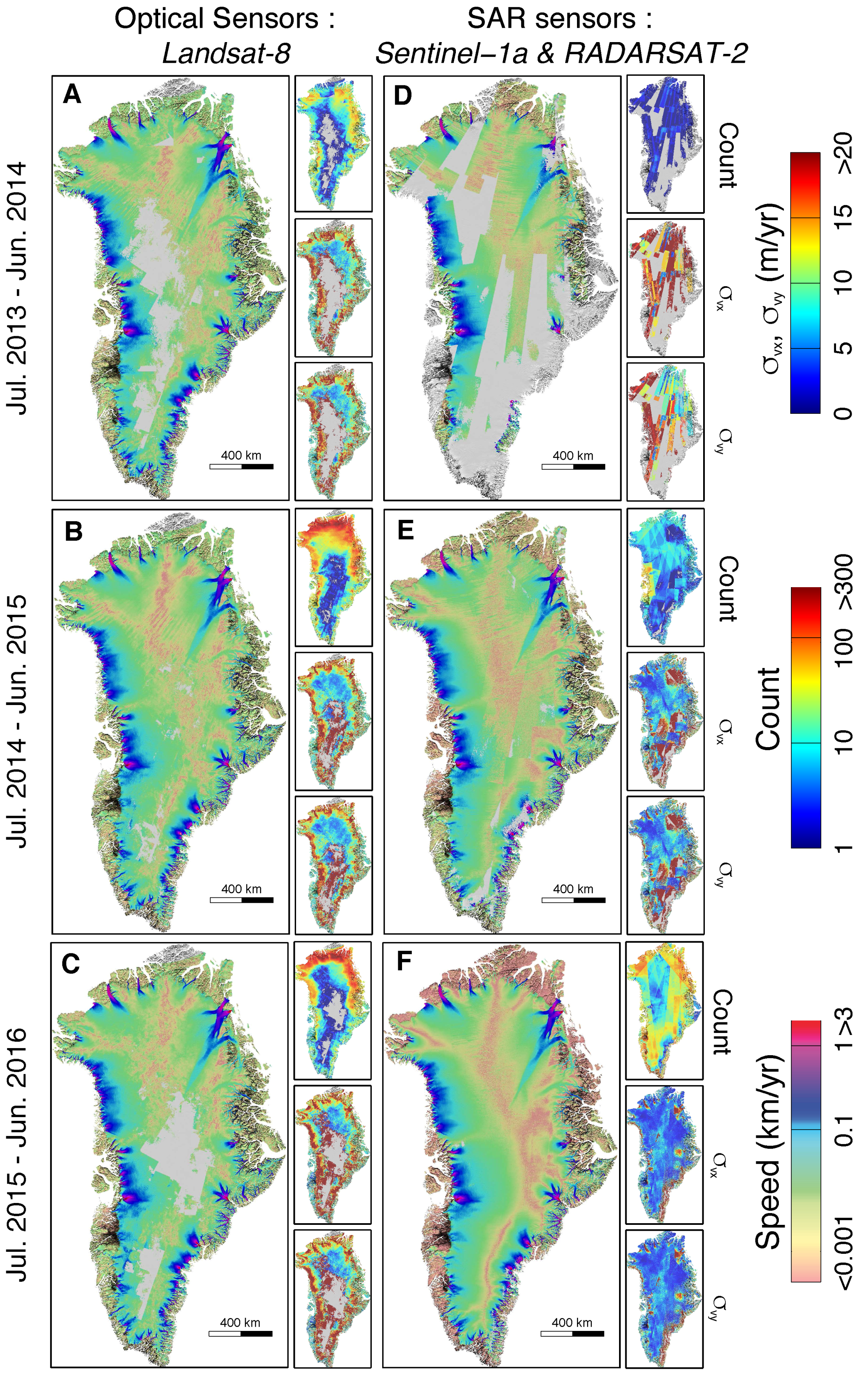
Figure 4.
Ice speed of Zachariae Isstrøm between 1992 and 2017 (A) and between 2014 and 2017 (B) from multiple sensors. Landsat prior to 2013 were downloaded from NSIDC [37].
Figure 4.
Ice speed of Zachariae Isstrøm between 1992 and 2017 (A) and between 2014 and 2017 (B) from multiple sensors. Landsat prior to 2013 were downloaded from NSIDC [37].
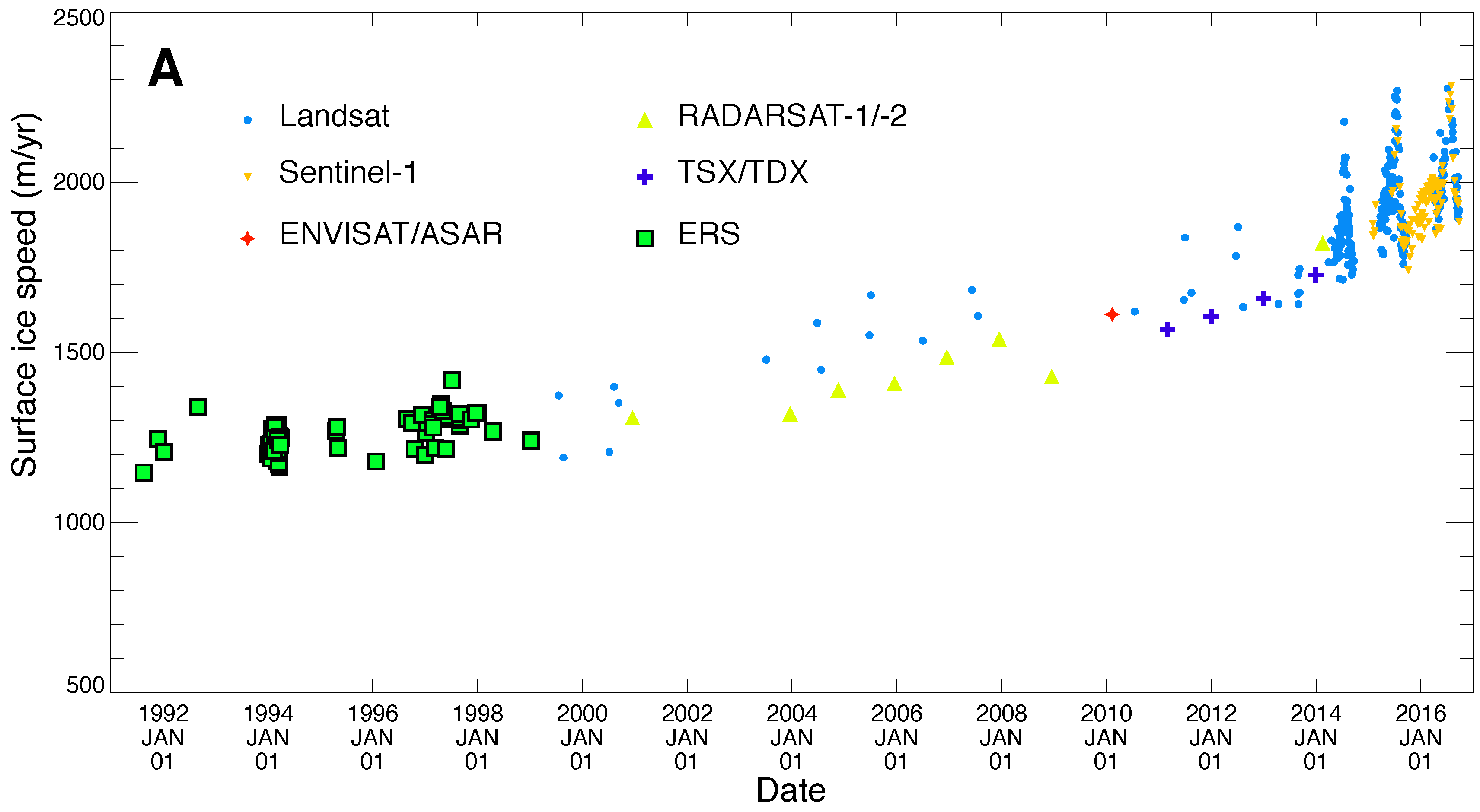

Figure 5.
Antarctic ice speed maps for each sensor and each cycle separately. The ice speed is coded on a logarithmic scale overlaid on MOA background mosaic.
Figure 5.
Antarctic ice speed maps for each sensor and each cycle separately. The ice speed is coded on a logarithmic scale overlaid on MOA background mosaic.
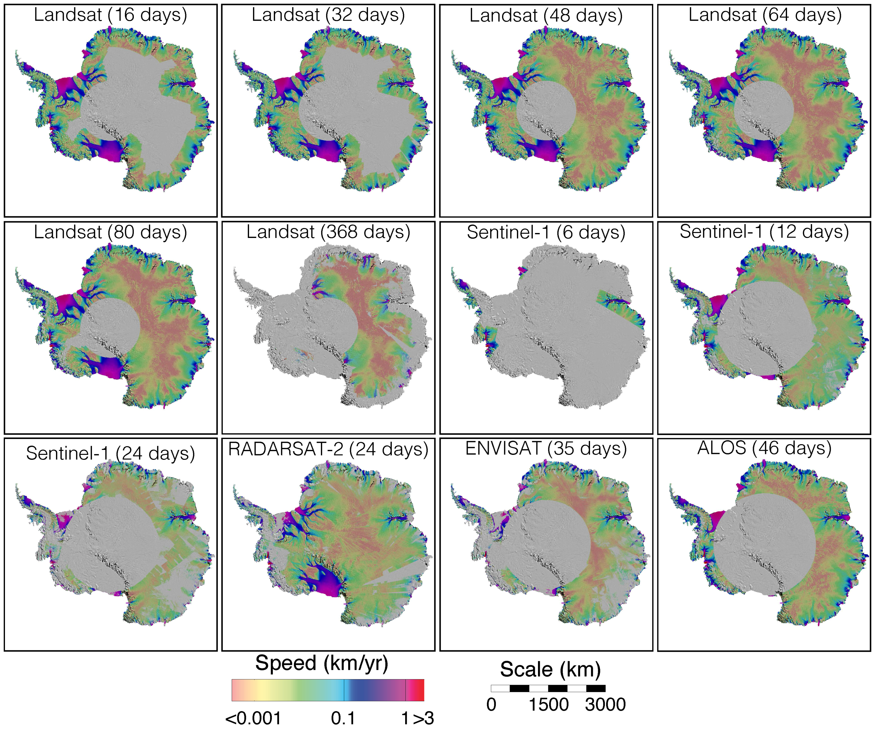
Figure 6.
(A) Lognormal distribution of the standard deviation of the antarctic ice velocity mosaics produced for each sensor and each repeat interval. For Landsat-8 (top-left panel), the 6 distributions correspond to repeat intervals of 368 (red), 80 (orange), 64 (green), 48 (turquoise), 32 (light blue) and 16 days (blue), respectively. SAR distributions are color-coded with greys getting darker with the length repeat cycle. Sentinel-1 (top-left panel) has 3 distributions for 6 (lightest), 12 and 24 (darkest) day repeat cycle. (B) Mode of the standard deviation distributions in (A) versus repeat interval. The grey vertical bars correspond to the 1-sigma deviation of the lognormal distributions shown in (A). Note: RADARSAT-2 point is shifted by 0.5 days to avoid overlapping with Sentinel-1 (24 days).
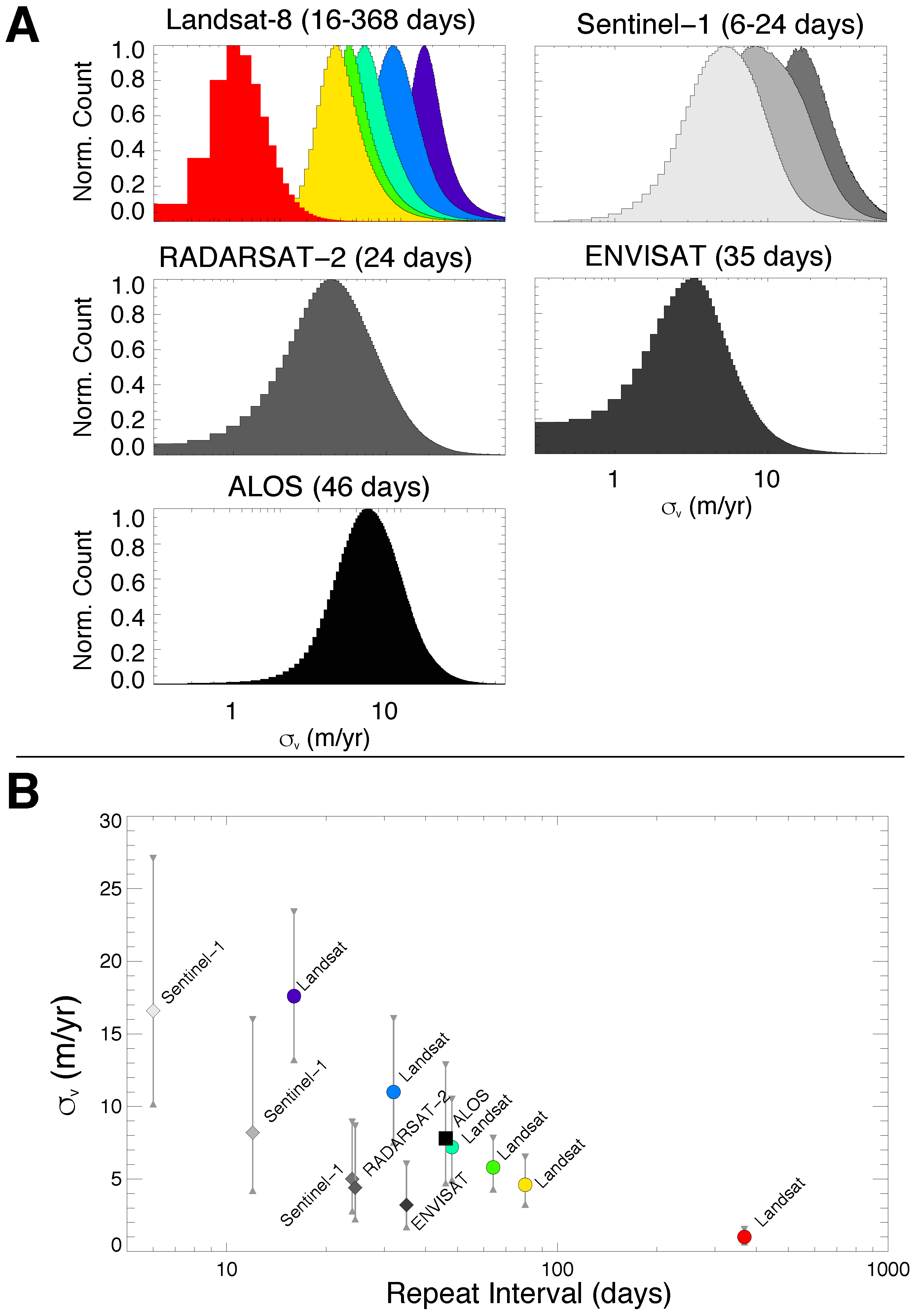
Figure 7.
Distribution of the difference between the velocity maps from Sentinel-1 and Landsat-8 for year 2014–2015. The velocity component and are displayed on the bottom and top panels, respectively.
Figure 7.
Distribution of the difference between the velocity maps from Sentinel-1 and Landsat-8 for year 2014–2015. The velocity component and are displayed on the bottom and top panels, respectively.
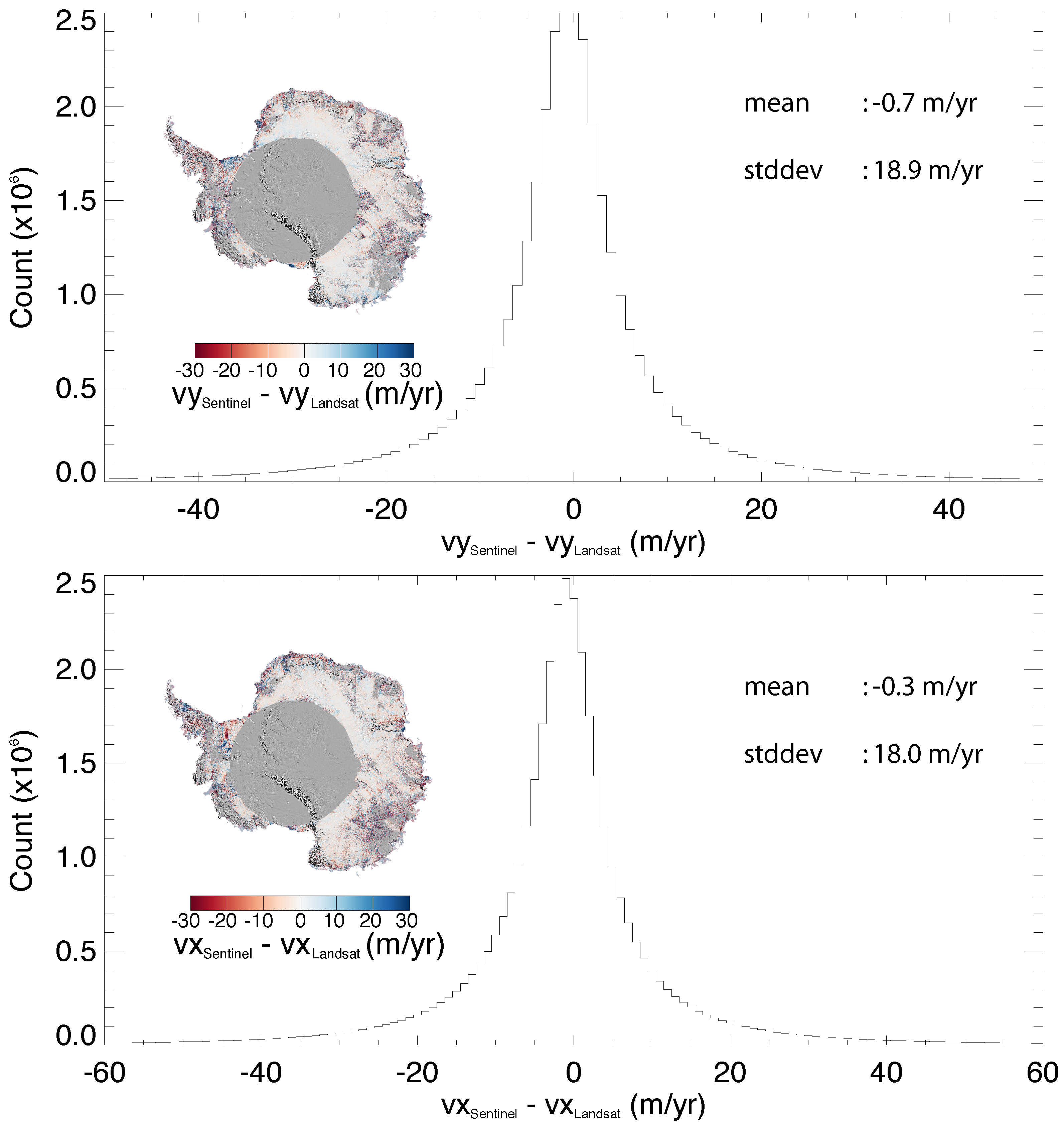
Figure 8.
Distribution of the difference between the ice velocity from ENVEO’s ice velocity [19] and the mosaics (this study) made from Landsat (Left) and Sentinel-1 (Right) for year 2014–2015 (Top) and year 2015–2016 (Bottom).
Figure 8.
Distribution of the difference between the ice velocity from ENVEO’s ice velocity [19] and the mosaics (this study) made from Landsat (Left) and Sentinel-1 (Right) for year 2014–2015 (Top) and year 2015–2016 (Bottom).
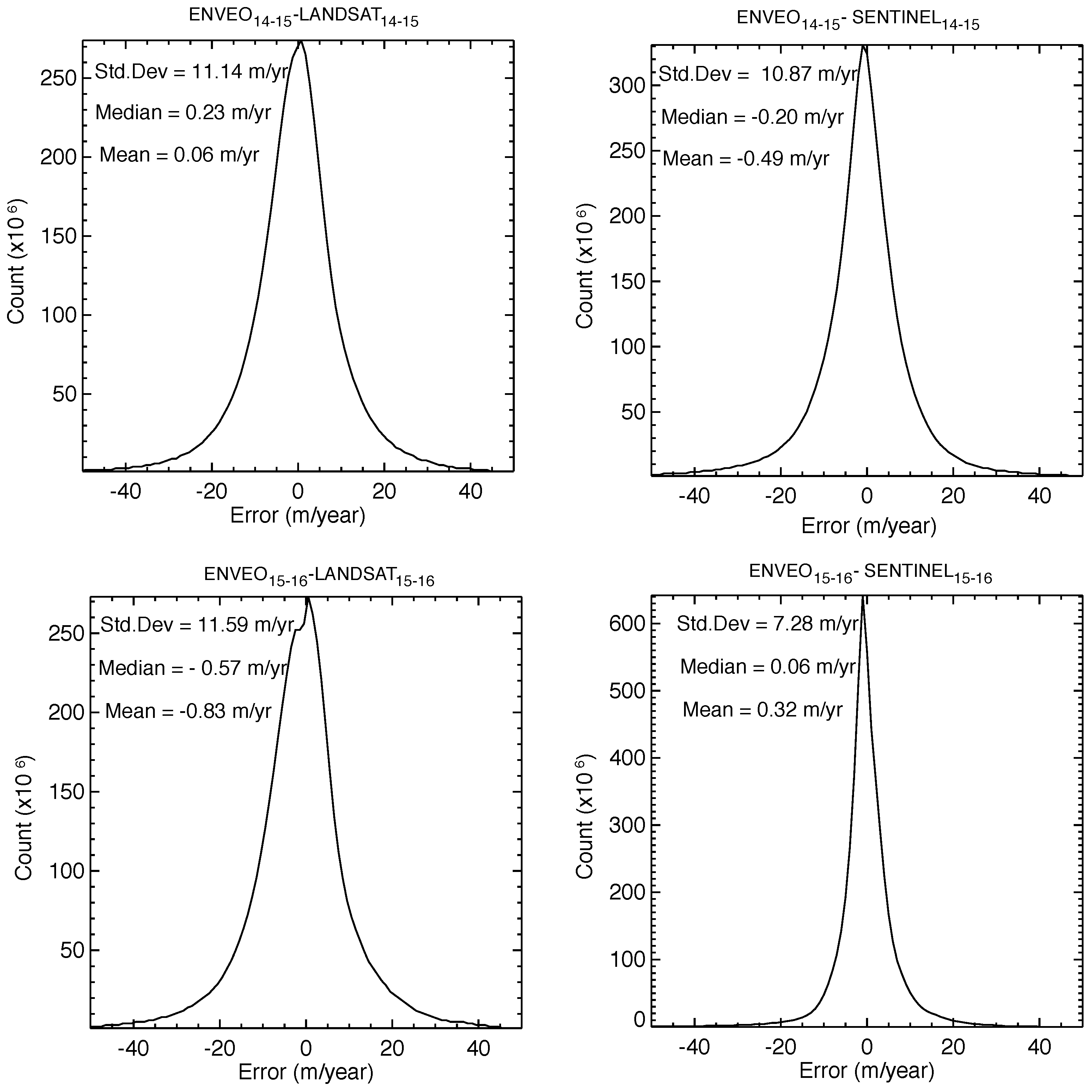
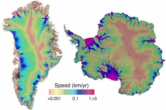
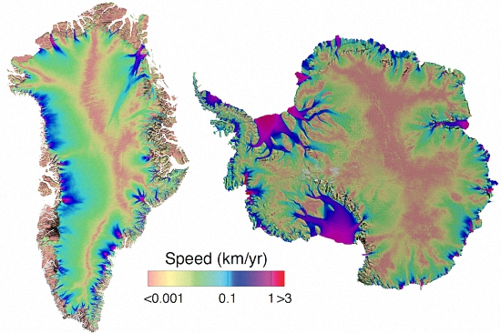
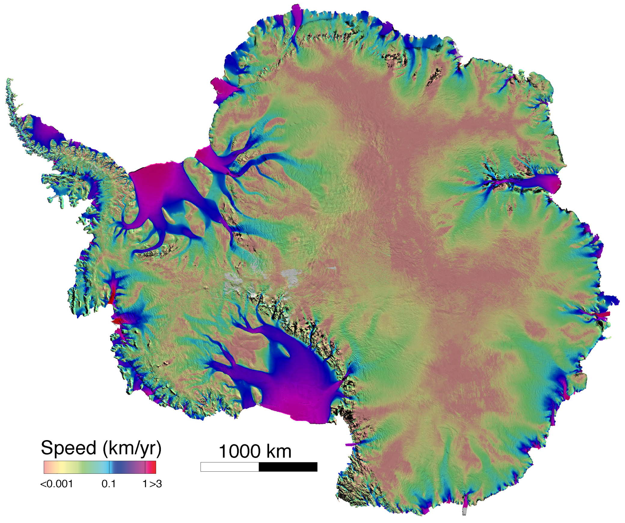
Figure 9.
Composite mosaic of surface ice speed generated from ERS-1&-2/ESA, RADARSAT-1&-2/ CSA, ENVISAT/ESA, ALOS/JAXA, TerraSAR-X/DLR, Sentinel-1/ESA and Landsat-8/USGS in Antarctica acquired between 1992 and 2016. The ice speed is coded on a logarithmic scale overlaid on MOA background mosaic [32].

Figure 10.
Composite mosaic of surface ice speed generated from ERS-1&-2/ESA, RADARSAT-1&-2/ CSA, ENVISAT/ESA, ALOS/JAXA, TerraSAR-X/DLR, Sentinel-1/ESA and Landsat-8/USGS acquired between 1992 and 2016 in Greenland. The ice speed is coded on a logarithmic scale overlaid on MOG background mosaic [33].

Table 1.
Ice velocity mapping precision () for different sensors assuming an error in measured displacement of 0.1 pixel, calculated as where is the pixel size in meters and is the repeat cycle in days. RADARSAT-1/&-2 precision may vary depending on the acquisition mode, we use here the values for the most common mode in our dataset. The precision is affected by the nominal repeat orbit as well as the resolution, this table is therefore provided for reference only. We show in our work that actual precision is often better than that provided in Table 1. The utility of the table lies in a cross sensor comparison, that we exploit in our weighting system when we form the velocity mosaic. Text in italics indicates values for sensors used in previous studies [2,22,27].
| Resolution | Nominal Repeat | Ice Vel. | |
|---|---|---|---|
| Rg. × Az. (m) | Cycle (days) | Precision (m/year) | |
| Landsat-8 | 15 × 15 | 16 | 34.2 × 34.2 |
| Sentinel-1 | 4 × 14 | 12 | 12.2 × 42.6 |
| RADARSAT-2 | 17 × 5 | 24 | 25.8 × 7.6 |
| ENVISAT/ASAR | 20 × 4 | 35 | 20.8 × 4.2 |
| ALOS/PALSAR | 7 × 3 | 46 | 5.5 × 2.4 |
| RADARSAT-1 | 17 × 5 | 24 | 25.8 × 7.6 |
© 2017 by the authors. Licensee MDPI, Basel, Switzerland. This article is an open access article distributed under the terms and conditions of the Creative Commons Attribution (CC BY) license (http://creativecommons.org/licenses/by/4.0/).
Share and Cite
MDPI and ACS Style
Mouginot, J.; Rignot, E.; Scheuchl, B.; Millan, R. Comprehensive Annual Ice Sheet Velocity Mapping Using Landsat-8, Sentinel-1, and RADARSAT-2 Data. Remote Sens. 2017, 9, 364. https://doi.org/10.3390/rs9040364
AMA Style
Mouginot J, Rignot E, Scheuchl B, Millan R. Comprehensive Annual Ice Sheet Velocity Mapping Using Landsat-8, Sentinel-1, and RADARSAT-2 Data. Remote Sensing. 2017; 9(4):364. https://doi.org/10.3390/rs9040364
Chicago/Turabian StyleMouginot, Jeremie, Eric Rignot, Bernd Scheuchl, and Romain Millan. 2017. "Comprehensive Annual Ice Sheet Velocity Mapping Using Landsat-8, Sentinel-1, and RADARSAT-2 Data" Remote Sensing 9, no. 4: 364. https://doi.org/10.3390/rs9040364
Note that from the first issue of 2016, this journal uses article numbers instead of page numbers. See further details here.