Spaceborne GNSS-R from the SMAP Mission: First Assessment of Polarimetric Scatterometry over Land and Cryosphere

Abstract

This work describes the first global scale assessment of a Global Navigation Satellite Systems Reflectometry (GNSS-R) experiment performed on-board the Soil Moisture Active Passive (SMAP) mission for soil moisture and biomass determination. Scattered GPS L2 signals (1227.6 MHz) were collected by the SMAP’s dual-polarization (Horizontal H and Vertical V) radar receiver and then processed on-ground using a known replica of the GPS L2C code. The scattering properties over land are evaluated using the Signal-to-Noise Ratio ($\mathrm{SNR}$), the Polarimetric Ratio ($\mathrm{PR}$), and the width of the waveforms’ trailing and leading edges. These parameters show sensitivity to the effects of the Earth’s topography and Above Ground Biomass (ABG) even over Amazonian and Boreal forests. These effects are shown to be an important factor in precise soil moisture and biomass determination. Additionally, it is found that $\mathrm{PR}$ shows sensitivity to soil moisture content over different land cover types. In particular, the following values of the PR are found over: (a) tropical forests ~−1.2 dB; (b) boreal forests ~0.8 dB; (c) Greenland ~2.8 dB; and (d) the Sahara Desert ~3.2 dB.

1. Introduction

The concept of multistatic scatterometry was proposed by Hall and Cordey in 1988 [1]. GNSS-R is an Earth Remote Sensing technique that exploits the signals transmitted by the Global Navigation Satellite Systems and hence can provide a dense global coverage of the Earth’s surface with rapid revisit time. It was originally proposed in 1993 by Martin-Neira for mesoscale ocean altimetry [2,3] to improve the spatio-temporal sampling of conventional nadir-looking radar missions. During the last decades, several ground-based [4], airborne, [5] and balloon [6] experiments have been carried out to demonstrate the feasibility of this technique for ocean altimetry and scatterometry. At present, GNSS-R ocean scatterometry applications are quite mature. On the other hand, the bistatic scattering properties over land surfaces deserve further study to evaluate the performance of this technique for soil moisture determination and biomass monitoring.

The first space-borne opportunistic measurement of an Earth-reflected GPS signal took place during the Space-borne Imaging Radar-C (SIR-C) mission in 1994 [7]. The first designed experiment of GNSS Reflectometry from space took place on-board the United Kingdom UK-DMC in 2003 [8].

The UK-TechDemoSat-1 using a Surrey Satellite Technology Ltd. (SSTL) receiver was launched in June 2014, providing useful GPS L1 C/A code data sets for the GNSS-R community [9]. Researchers, have studied the sensitivity of GNSS-R for soil moisture determination [10,11], ocean altimetry [12] and scatterometry [13,14], and sea ice detection [15]. More recently, the 6U cubesat ³Cat-2 [16] developed by the Universitat Politecnica de Catalunya (UPC) was launched on 15 August 2016, and NASA’s Cyclone Global Navigation Satellite System (CyGNSS) GPS L1 C/A code-based constellation was recently launched on 15 December 2016 [17], providing an unprecedented sampling of the Earth’s surface.

In 2000, the use of polarimetric GNSS-R was first proposed by Zavorotny for soil moisture determination [18]. At present, there are two main approaches for soil moisture determination with GNSS-R: (i) the first uses tower-based geodetic GNSS receivers and the multipath Signal-to-Noise Ratio ($\mathrm{SNR}$) to retrieve ground moisture [4,19,20] in a small region around the tower; (ii) the second one uses specifically designed receivers and two antennas either at Left and Right Hand Circular Polarizations (LHCP and RHCP) as in [21,22,23], or at horizontal H and vertical V polarizations as in [24]. The second technique using an horizontal H-Pol and V-Pol antenna is used in this work. Theoretical [25,26] and experimental [27] assessments have shown a sensitivity to forest biomass. Recent airborne [21] and stratospheric balloon [28] flight experiments have been performed using new instruments and circular polarization antennas (RHCP and LHCP) for geophysical parameter retrieval over land surfaces, and wetlands. These experiments have shown the capability of GNSS-R techniques for wetlands monitoring even from high altitude platforms (~27 km) [28] because of the high spatial resolution provided by the coherent component of the scattered field.

This study presents results from a serendipitous GNSS-R experiment performed on-board the SMAP mission [29] over continental areas. This unique data set, which provides very high-gain GPS L2C code dual-polarization (H and V) sampling of the Earth’s surface up to high latitudes, is evaluated to assess the behaviour of different parameters of the so-called reflected waveforms corresponding to Soil Water Index (SWI), Normalized Difference Vegetation Index (NDVI), Above Ground Biomass (AGB), and topography. Section 2 describes the methodology and the experiment set-up. Section 3 presents the results, Section 4 provides final discussions, and the main conclusions are highlighted in Section 5.

2. Description of the GNSS-R Experiment

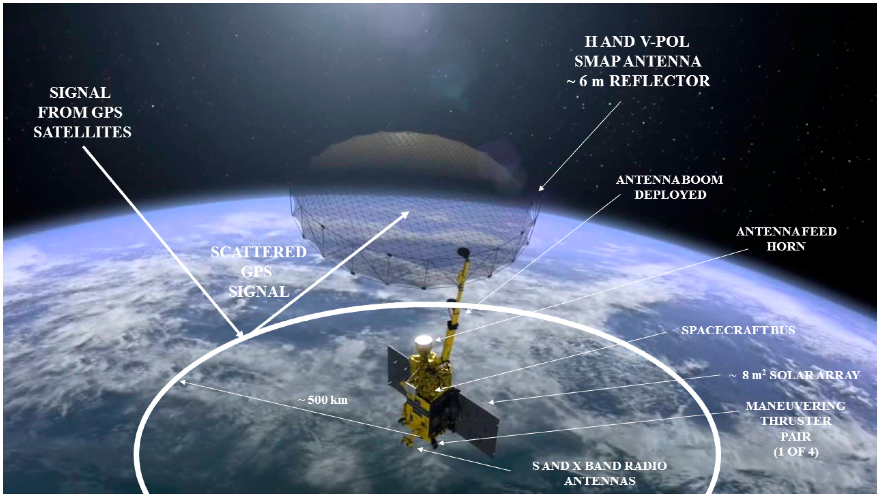
The SMAP mission was successfully launched on 31 January 2015 into a Sun-Synchronous Orbit (SSO) with a local time of ascending node (LTAN) of 6:00 h, and an orbit height of ~685 km. The main mission instruments are an active L-band radar and a passive radiometer which share a ~14 rev/min rotating 6-m aperture reflector antenna scanning a wide 1000 km wide swath (Figure 1 and Figure 2). The dual-polarization reflector (H and V) points to Earth’s surface with an approximately fixed elevation angle of ${\mathsf{\theta }}_{\mathrm{e}}$ ~55°. The elevation angle of the collected signals was approximately constant ~55° during the complete experiment because the attitude of the SMAP satellite is the same in nominal operations. Data acquisition used a 50 km cut on (footprint area ~7800 km²) the closest approach to the specular point, and calibrated using the antenna radiation pattern. This possibly is cutting off the waveform trailing edge over some regions. 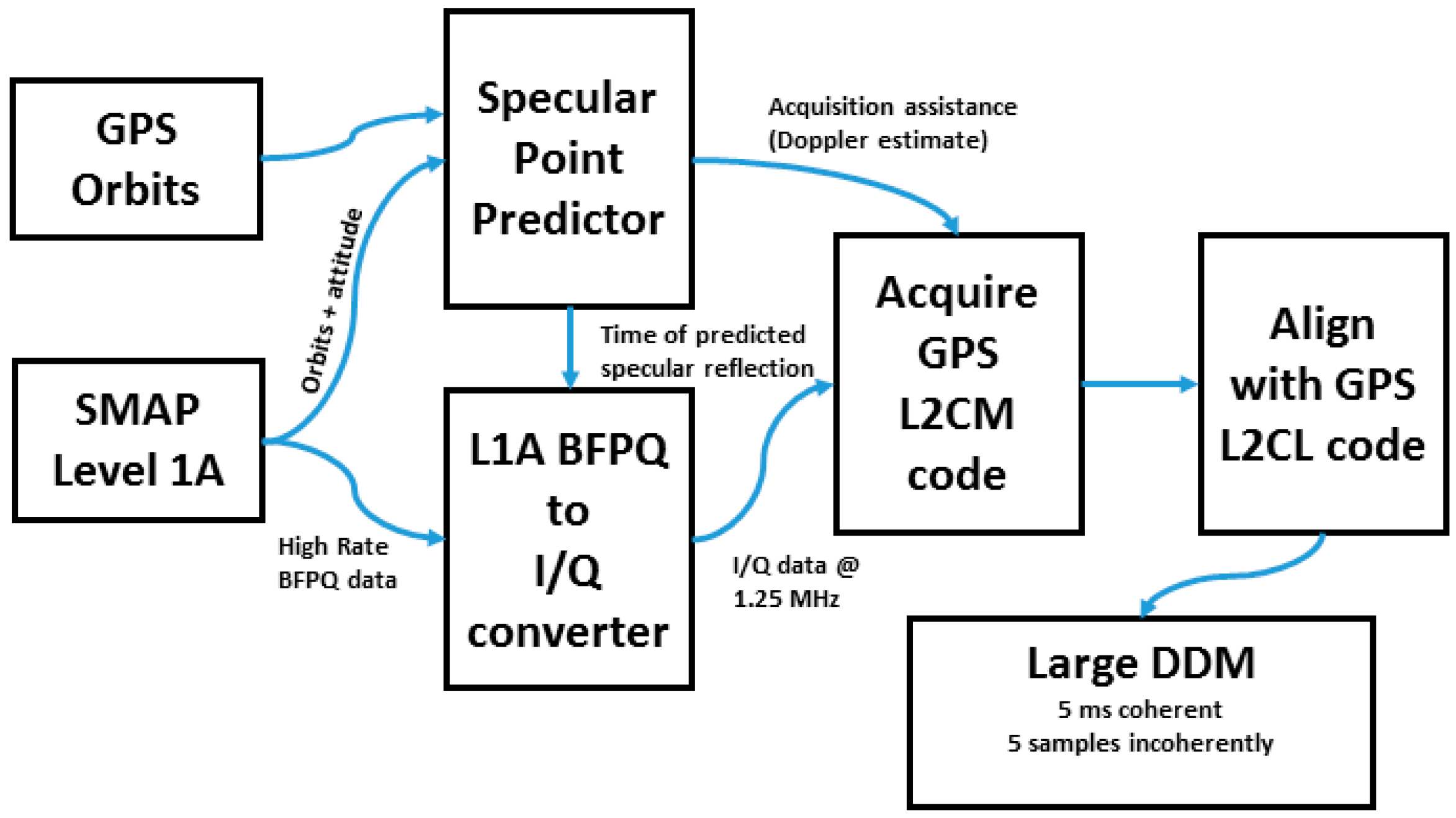Figure 3 shows enough sensitivity from Greenland to tropical forests. The High-Power Amplifier (HPA) failed on 7 July 2015, preventing the emission of radar pulses and thus the use of the instrument as an active device. As an experiment of opportunity, the radar receiver was tuned to the GPS L2 frequency (1227.6 MHz) in order to collect Earth-reflected GPS signals. Raw data were downloaded to the ground and then a geometric model was used to select SMAP’s Level L1 A binary data (orbit, attitude, antenna pointing, etc.) extraction from their archive to only those time periods with potential specular reflections (Figure 2). These data, combined with GPS orbital information, were used to predict when the SMAP’s antenna pointed to a nominal specular reflection point. This timing information was then used by a L1 A Block Floating Point Quantization (BFPQ) for In-phase (I) and Quadrature-phase (Q) conversion, where H-Pol and V-Pol data were extracted. This converter read in SMAP Level 1A data, and converted the compressed BFPQ numbers to I and Q 8-bit signed integers. These I/Q data had continuity gaps when the radar transmitter was supposed to be transmitting. The converter computed the required number of zero-valued samples to be inserted to provide a temporally continuous data set. These continuous I/Q samples were passed to the GPS L2 acquisition software, which searched in Doppler and delay for the L2 Civilian Medium-length code (L2CM), which repeats every 20 milliseconds. Once this code was found, the software aligned with the L2C Long code (L2CL), which repeats every 1.5 s. The precise Doppler and range information was passed on to the DDM processor, creating Delay Doppler Maps (DDMs) spanning ±10 kHz in Doppler and ±3000 km in range, and centered at the strongest detected signal, for both the H and V polarization data. After inspection, the data set was seen to be free of potential effects of Faraday rotation. Two signal peaks were selected because the direct GPS signal was almost always present in the data: timing between the two signals unambiguously determined which was the reflected signal used here. Finally, after averaging, power DDM’s $\langle {|{\mathrm{Y}}^{\mathrm{ref}}|}^2\rangle$ were obtained as a result [18,30]:

$$\langle {|{\mathrm{Y}}^{\mathrm{ref}}|}^2\rangle =\frac{{\mathrm{P}}_{\mathrm{t}}{\mathsf{\lambda }}^2}{{(4\mathsf{\pi })}^3}\iint \frac{{\mathrm{D}}_{\mathrm{T}}(\overrightarrow{\mathsf{\rho }}){\mathrm{D}}_{\mathrm{R}}(\overrightarrow{\mathsf{\rho }}){|\mathsf{\chi }(\mathsf{\tau }-({\mathrm{R}}_0+\mathrm{R})/\mathrm{c},{\mathrm{f}}_{\mathrm{D}}(\overrightarrow{\mathsf{\rho }})-{\mathrm{f}}_{\mathrm{c}})|}^2{\mathsf{\sigma }}^0(\overrightarrow{\mathsf{\rho }})}{{\mathrm{R}}_{\mathrm{T}}^2(\overrightarrow{\mathsf{\rho }}){\mathrm{R}}_{\mathrm{R}}^2(\overrightarrow{\mathsf{\rho }})}{\mathrm{d}}^2\mathsf{\rho },$$

(1)

where ${\mathrm{P}}_{\mathrm{t}}$ is the transmitted power, ${\mathrm{D}}_{\mathrm{T}}$ and ${\mathrm{D}}_{\mathrm{R}}$ are the transmitter and receiver antenna directivities at the point $\overrightarrow{\mathsf{\rho }}$ over the Earth’s surface, ${\mathrm{R}}_{\mathrm{T}}$ and ${\mathrm{R}}_{\mathrm{R}}$ are the distance from the transmitter and the receiver to point $\overrightarrow{\mathsf{\rho }}$, ${|\mathsf{\chi }(\mathsf{\tau },\mathrm{f})|}^2$ is the Woodward Ambiguity Function (WAF), and ${\mathsf{\sigma }}^0$ is scattering coefficient. The coherent integration time was set to ${\mathrm{T}}_{\mathrm{coh}}$ = 5 ms and the number of incoherent averaging ${\mathrm{N}}_{\mathrm{inc}}$ = 5 to increase the Signal-to-Noise Ratio ($\mathrm{SNR}$). Lower levels of ${\mathrm{T}}_{\mathrm{coh}}$ were tested, and it was found that ${\mathrm{T}}_{\mathrm{coh}}$ = 5 ms is the optimum for this experiment configuration. The spatial resolution associated to the waveforms’ peak is linked to the first Fresnel zone (~1 km²) in the case of specular scattering, and limited by the glistening zone in the case of the non-specular scattering, related to the area of the first iso-delay ellipse, that is ~1800 km²; plus the degradation due to: (a) the platform’s movement (in the SMAP’s case this degradation is $|{\overrightarrow{\mathrm{v}}}_{\mathrm{SMAP}}|\cdot {\mathrm{T}}_{\mathrm{c}}\cdot {\mathrm{N}}_{\mathrm{inc}}=7.48\mathrm{km}/\mathrm{s}\cdot 0.005\mathrm{s}\cdot 5=0.187\mathrm{km}$); (b) the antenna rotation; this degradation is unique to this scenario, and as a consequence the point at antenna boresight moves ~ 18 km during the integration time.

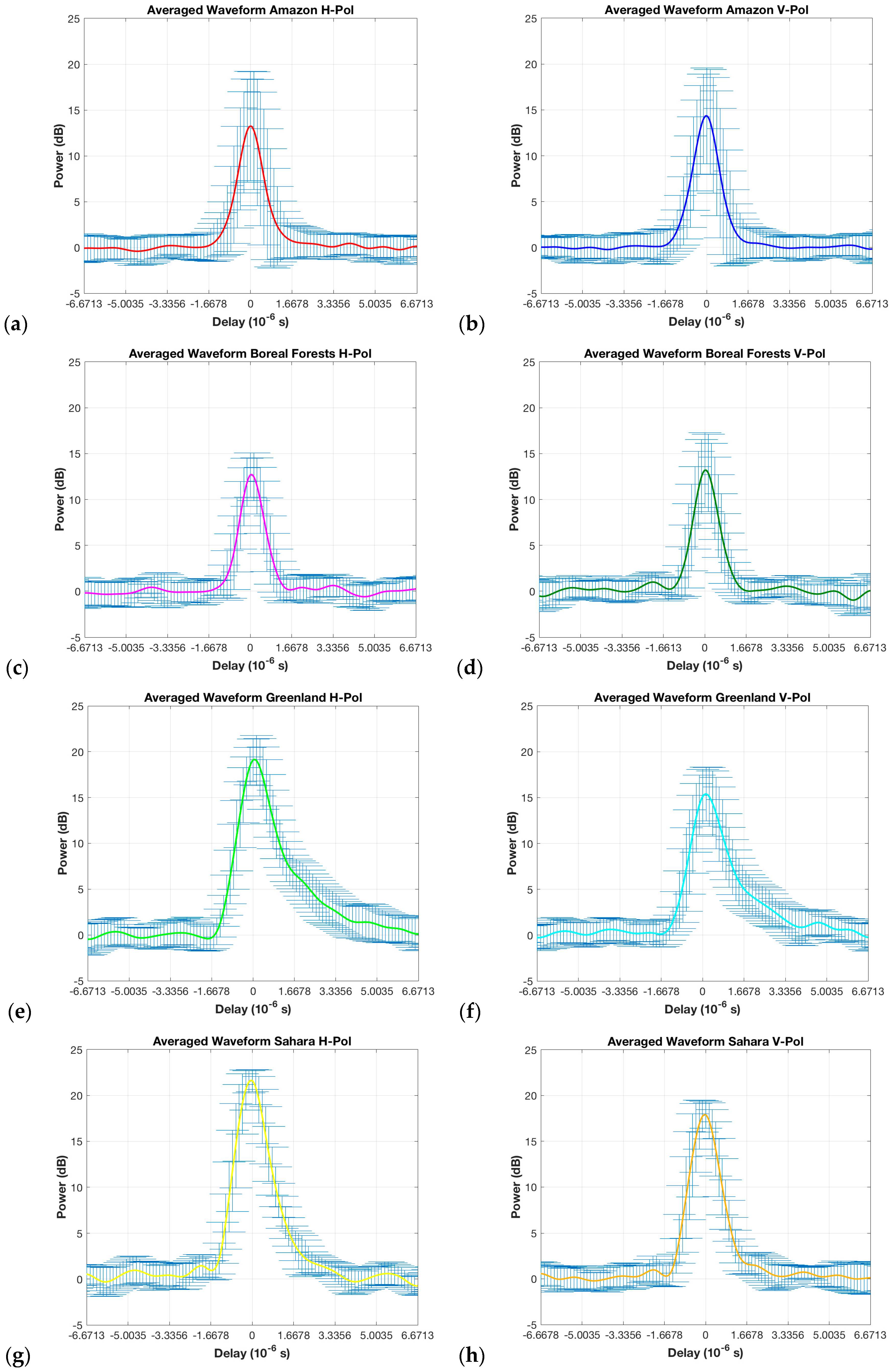
Waveforms corresponding to the Doppler central frequency were obtained for further assessment over land and cryosphere. Averaged waveforms with the associated RMS at each lag are represented in Figure 3 for both polarizations and different terrain types. To describe the shape of the waveforms quantitatively and to account for the power differences and spreading of the signal, the following parameters are used: Signal-to-Noise Ratio ($\mathrm{SNR}$), Polarimetric Ratio ($\mathrm{PR}$), and waveforms’ trailing and leading edges width.

The $\mathrm{SNR}$ is estimated as in [31], and defined as [3]:

$$\mathrm{SNR}=\frac{\langle {|{\mathrm{Y}}^{\mathrm{ref}}|}^2\rangle }{\langle {|{\mathrm{Y}}^{\mathrm{noise}}|}^2\rangle }=\frac{\langle {|{\mathrm{Y}}^{\mathrm{ref}}|}^2\rangle }{{\mathrm{k}}_{\mathrm{B}}\mathrm{TB}},$$

(2)

where ${\mathrm{k}}_{\mathrm{B}}$ is the Boltzmann constant, $\mathrm{T}$ is the equivalent noise temperature of the down-looking chain, and $\mathrm{B}$ is the signal bandwidth.

The Polarimetric Ratio ($\mathrm{PR}$) is computed to properly evaluate the fluctuations of the dielectric properties of scatterers, since theoretically it can cancel out the effects of soil surface roughness without biomass [18], although it does not do so perfectly for arbitrary scattering media. The PR at linear polarization is high when soil moisture content is weak and reversely. On the other hand, at circular polarization the ratio increases with the moisture [18]. It is estimated as the ratio of the peak of the reflected signal power waveform at H-Pol over the peak of the reflected signal power waveform at V-Pol, after proper compensation of the noise power floor and the antenna radiation pattern:

$$\mathrm{PR}=\frac{\langle {|{\mathrm{Y}}_{\mathrm{H}}^{\mathrm{ref}}|}^2\rangle }{\langle {|{\mathrm{Y}}_{\mathrm{V}}^{\mathrm{ref}}|}^2\rangle }.$$

(3)

The theoretical definition of the $\mathrm{PR}$ is provided in [32] as:

$$\mathrm{PR}={\mathsf{\sigma }}_{\mathrm{H}}/{\mathsf{\sigma }}_{\mathrm{V}},$$

(4)

where ${\mathsf{\sigma }}_{\mathrm{H}}$ and ${\mathsf{\sigma }}_{\mathrm{V}}$ are the bistatic radar cross-sections of H and V respectively.

Over land surfaces, there are two contributions to the waveforms: coherent and incoherent scattered fields in different proportions. In this scenario, the Kirchhoff Approximation in the Physical Optics Approximation (KPO) provides a reasonable theoretical framework to analyze the results in regions without biomass. The incoherent bistatic scattering coefficient as provided by the KPO is [33]:

$${\mathsf{\sigma }}_{\mathrm{qp}}^{0,\mathrm{inc}}={(|{\mathrm{a}}_0|\mathrm{k}l/2)}^2{\mathrm{e}}^{-{\mathrm{q}}_{\mathrm{z}}^2{\mathsf{\sigma }}^2}{\displaystyle \sum }_{\mathrm{n}=1}^{\infty }\frac{({\mathrm{q}}_{\mathrm{z}}^2{\mathsf{\sigma }}^2)}{\mathrm{n}!\mathrm{n}}{\mathrm{e}}^{-\frac{({\mathrm{q}}_{\mathrm{x}}^2+{\mathrm{q}}_{\mathrm{y}}^2)l^2}{4\mathrm{n}}},$$

(5)

where $\mathrm{k}=\raisebox{1ex}{$2\mathsf{\pi }$}\!\left/ \!\raisebox{-1ex}{$\mathsf{\lambda }$}\right.$, $l$ is the surface correlation length, $\mathsf{\sigma }$ is the surface height standard deviation, and $\overrightarrow{\mathrm{q}}$ is the bistatic scattering coefficient. In the specular direction, the coefficient ${\mathrm{a}}_0$ can be computed for the co-polar component H:

$${\mathrm{a}}_{0,\mathrm{H}}=-2{\mathrm{R}}_{\mathrm{H}}({\mathsf{\theta }}_{\mathrm{inc}}){\cos \mathsf{\theta }}_{\mathrm{inc}},$$

(6)

and for the co-polar component V:

$${\mathrm{a}}_{0,\mathrm{V}}=2{\mathrm{R}}_{\mathrm{V}}({\mathsf{\theta }}_{\mathrm{inc}}){\cos \mathsf{\theta }}_{\mathrm{inc}},$$

(7)

where ${\mathsf{\theta }}_{\mathrm{inc}}$ is the incidence angle, and ${\mathrm{R}}_{\mathrm{H}}$ and ${\mathrm{R}}_{\mathrm{V}}$ are the Fresnel reflection coefficients at H-Pol and V-Pol respectively:

$${\mathrm{R}}_{\mathrm{H}}=\frac{\sqrt{1-{\sin }^2({\mathsf{\theta }}_{\mathrm{inc}})}-\sqrt{{\mathsf{\epsilon }}_{\mathrm{r}}-{\sin }^2({\mathsf{\theta }}_{\mathrm{inc}})}}{\sqrt{1-{\sin }^2({\mathsf{\theta }}_{\mathrm{inc}})}+\sqrt{{\mathsf{\epsilon }}_{\mathrm{r}}-{\sin }^2({\mathsf{\theta }}_{\mathrm{inc}})}},$$

(8)

and

$${\mathrm{R}}_{\mathrm{V}}=\frac{{\mathsf{\epsilon }}_{\mathrm{r}}\sqrt{1-{\sin }^2({\mathsf{\theta }}_{\mathrm{inc}})}-\sqrt{{\mathsf{\epsilon }}_{\mathrm{r}}-{\sin }^2({\mathsf{\theta }}_{\mathrm{inc}})}}{{\mathsf{\epsilon }}_{\mathrm{r}}\sqrt{1-{\sin }^2({\mathsf{\theta }}_{\mathrm{inc}})}+\sqrt{{\mathsf{\epsilon }}_{\mathrm{r}}-{\sin }^2({\mathsf{\theta }}_{\mathrm{inc}})}},$$

(9)

where ${\mathsf{\epsilon }}_{\mathrm{r}}$ is the dielectric constant. For the cross-polar components HV and VH, ${\mathrm{a}}_0$ = 0 [33]. Therefore, upon substitution of (5), (6) and (7) in (4), the Polarimetric Ratio is found to be independent of the surface roughness:

$$\mathrm{PR}=\raisebox{1ex}{${\mathrm{R}}_{\mathrm{H}}$}\!\left/ \!\raisebox{-1ex}{${\mathrm{R}}_{\mathrm{V}}$}\right..$$

(10)

In the case of the coherent component of the scattered field [33] (p. 1008), the $\mathrm{PR}$ is obtained as the ratio of the H reflectivity over the V reflectivity as:

$$\mathrm{PR}=\raisebox{1ex}{${\mathrm{\Gamma }}_{\mathrm{H}}$}\!\left/ \!\raisebox{-1ex}{${\mathrm{\Gamma }}_{\mathrm{V}}$}\right.=\frac{{|{\mathrm{R}}_{\mathrm{H}}|}^2{\mathrm{e}}^{-{(2{\mathsf{\sigma }\mathrm{kcos}\mathsf{\theta }}_{\mathrm{inc}})}^2}}{{|{\mathrm{R}}_{\mathrm{V}}|}^2{\mathrm{e}}^{-{(2{\mathsf{\sigma }\mathrm{kcos}\mathsf{\theta }}_{\mathrm{inc}})}^2}},$$

(11)

Equation (11) shows that in the case of the coherent scattering, the $\mathrm{PR}$ is also theoretically independent of the soil surface roughness because the surface height standard deviation is independent of the signal polarization.

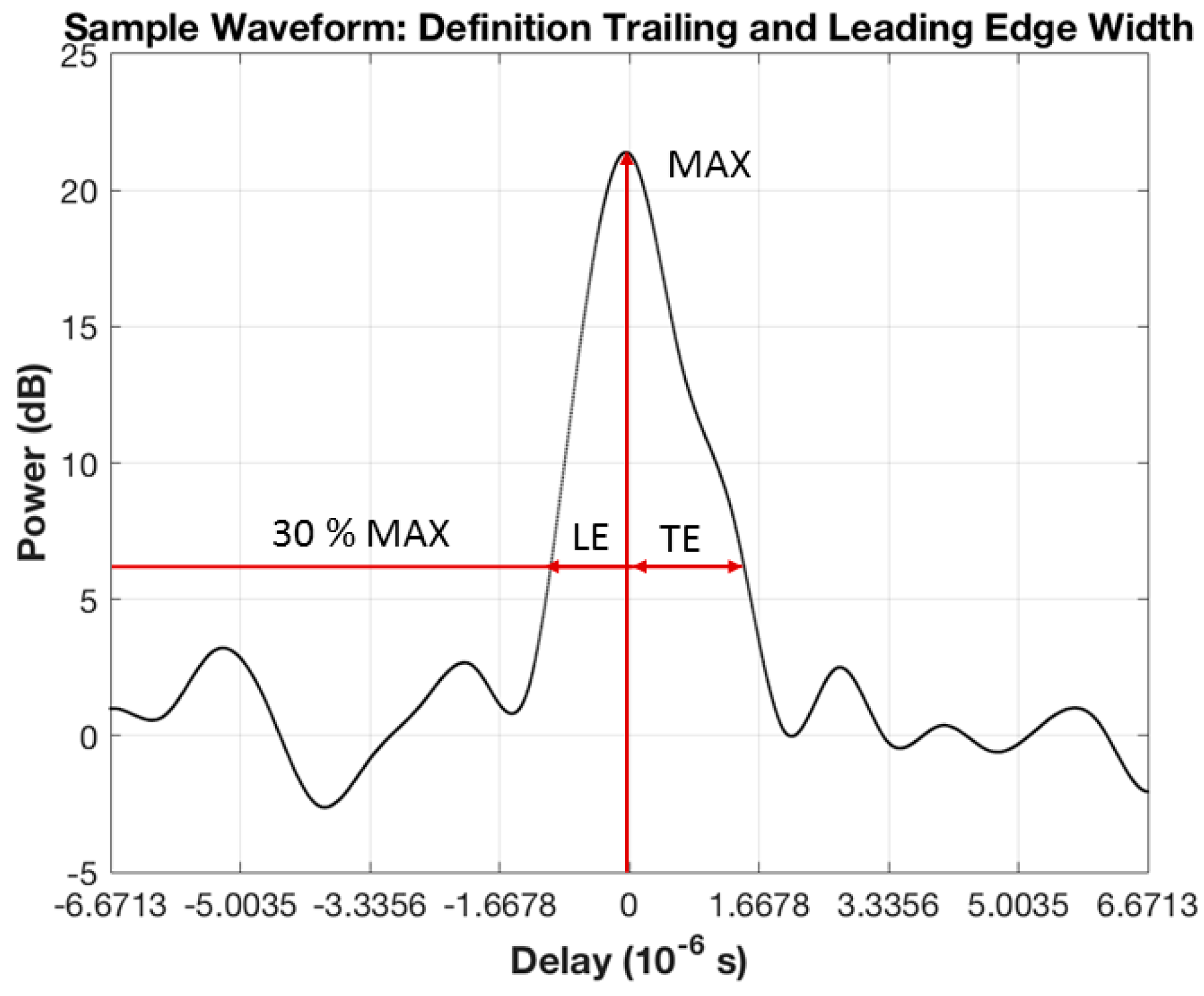
The width of both edges was defined as the lag difference between the 30% and the 100% of the maximum power of the waveform (Figure 4). Finally, it is highlighted that the generated SMAP GNSS-R dataset provided a unique opportunity for research in GNSS-R, despite this mission being designed for a different goal, because the SMAP’s radar receiver allowed the collection of reflected GNSS signals al L2, through the use of a high gain antenna ~36 dB. The observables (SNR, PR, and trailing and leading edges) will be used to analyze the reflected waveforms (Figure 3). In this figure, significant differences are seen among different areas. One of the most surprising results is the large spreading of the waveforms over Greenland and the large SNR over the Sahara Desert. These points will be further discussed in Section 3.

3. Earth Surface Effects on GNSS-R Relevant to Land Applications

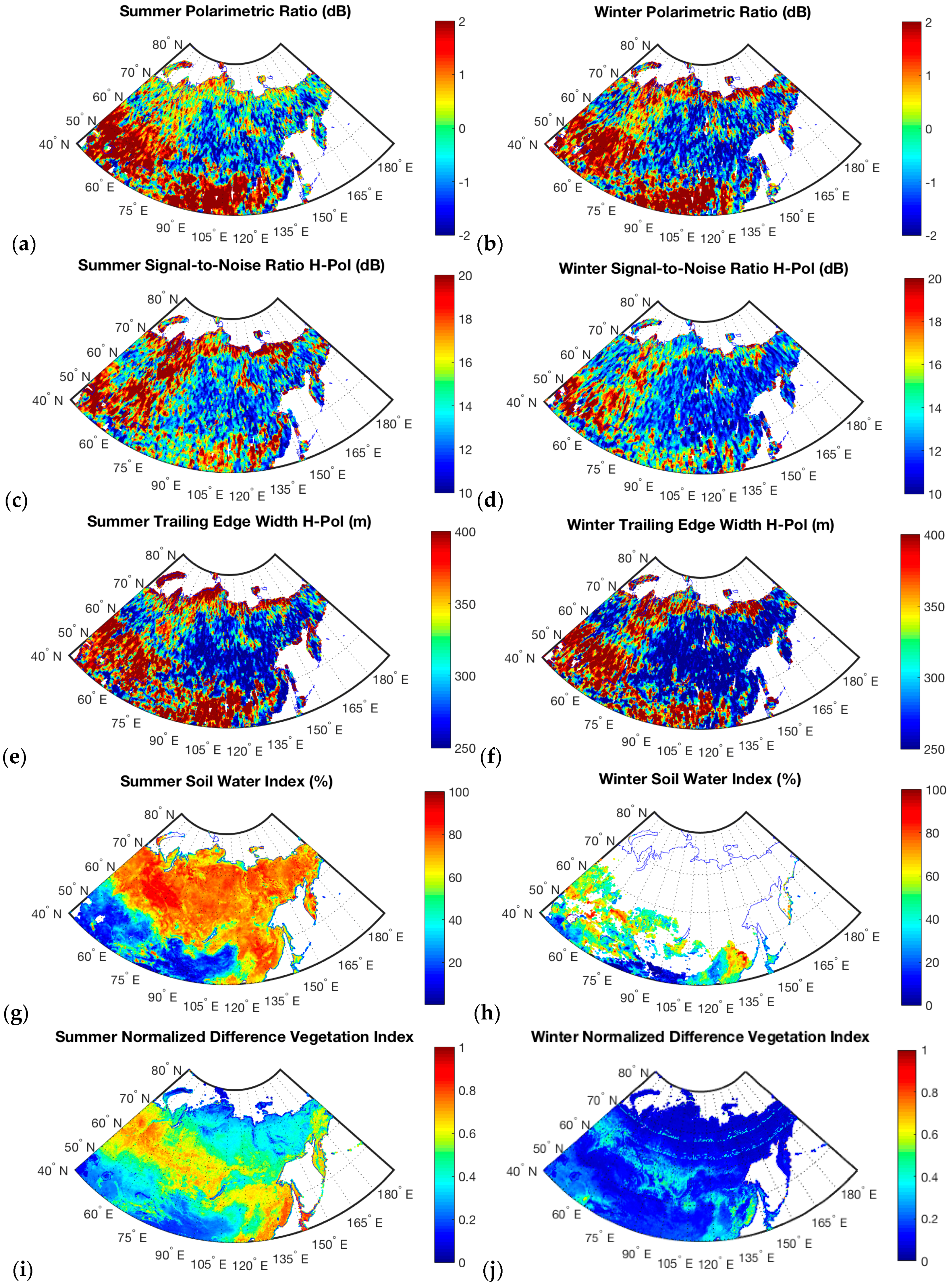
The potential of spaceborne GNSS-R for land applications is evaluated, first at a global scale and then at a regional scale. The results are displayed in a 0.1° latitude/longitude grid with a 1° pixel size used in the spatial averaging, performed with steps of 0.1°. The total number of observations over land surfaces is ~35,000 per month (~70,000 considering direct and reflected signals), and the maps are constructed using a mean value of ~25 ± 4 measurements per pixel. There are more data availability over target areas at larger latitude than over the equator because of the SMAP’s orbit parameters (polar orbit). On the other hand, the area of the selected pixel size gradually reduces from the equator to the poles. The lat/lon grid was selected to homogenize the number of measurements per pixel. In the close up over Africa, the selected spatial averaging size was 2°, also performed with steps of 0.1°. The pixel size was selected to be larger than that of global averaged maps because of the of lower data availability. The waveforms’ parameters ($\mathrm{SNR}$, $\mathrm{PR}$, and trailing & leading edges) are geo-located over the specular points on the Earth’s surface. Four different relatively “homogeneous” areas are considered to study statistically the waveforms’ properties associated with different scattering mechanisms. In particular, the coordinates of these regions are: (a) tropical forests: latitude = (−3, 3)° by longitude = (15, 25)°; (b) boreal forests: latitude = (50, 70)° by longitude = (90, 140)°; (c) Greenland: latitude = (75, 83)° by longitude = (−53, −31)°; and (d) Sahara Desert: latitude = (19, 28)° by longitude = (−7, 27)°. Four different three-months seasons (January–March, April–June, July–September, and October–December) have been selected to analyze the effect of seasonal variations at a regional scale on soil moisture and vegetation water content.

3.1. Global Scale

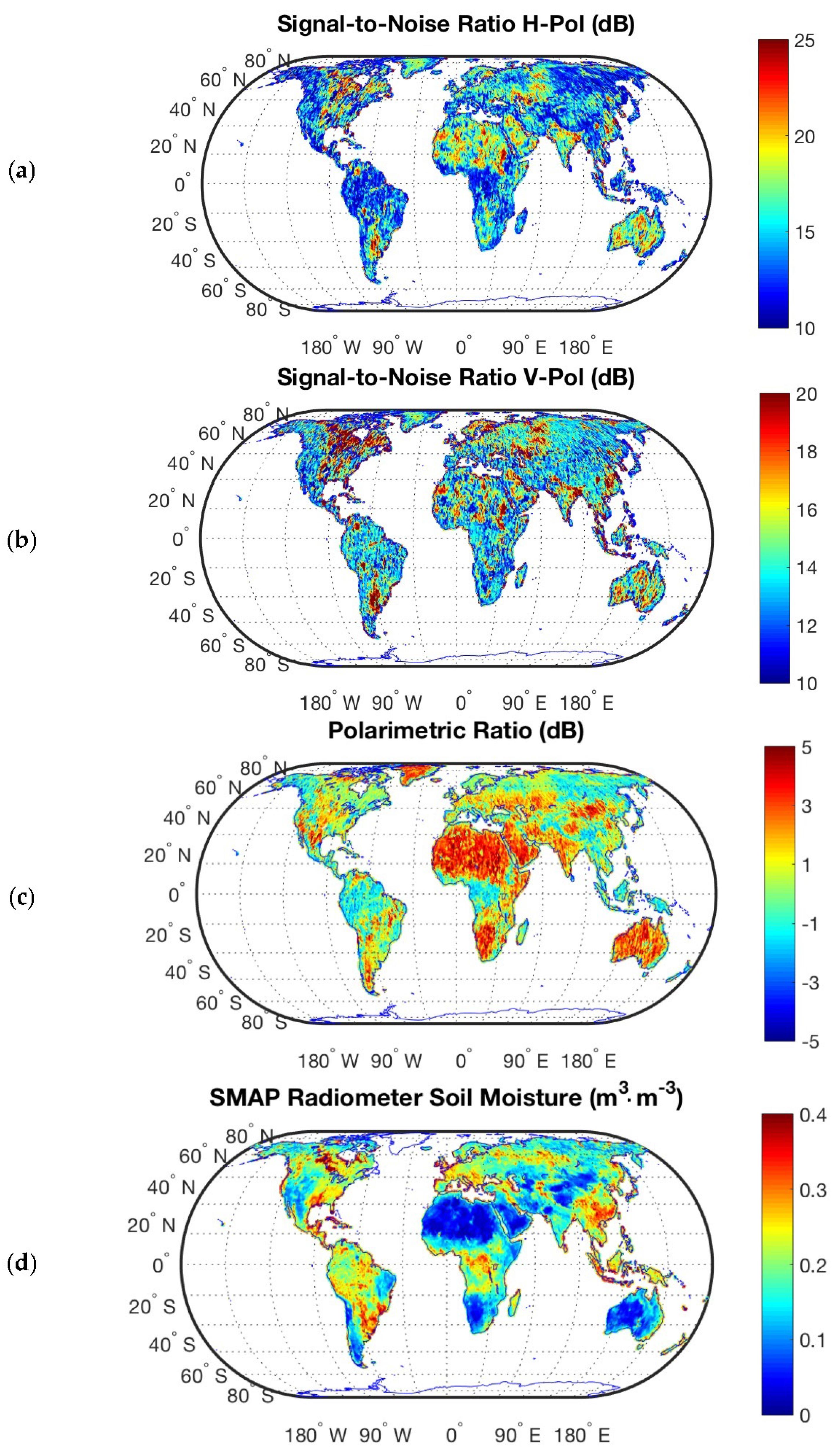
The global one-year averaged maps (1 September 2015 to 1 September 2016) provided in this study are useful for the global scale study. Signal-to-Noise Ratio ($\mathrm{SNR}$) values are presented for H-Pol and V-Pol respectively in Figure 5a,b over the Earth’s land surface. High $\mathrm{SNR}$ peaks correspond to bare soil regions with high soil moisture content such as the Pampas of Argentine, the Great Lakes regions in the US, Northern India, or the Northern Yakutia region in Russia. There are also high power peaks over regions such as the Sahara Desert despite the low soil moisture values. This effect will be investigated at a regional scale. In regions with significant amount of AGB, the $\mathrm{SNR}$ values are lower despite high values of soil moisture content because of the effect of signal attenuation (Figure 5a,b). The $\mathrm{PR}$ values (Figure 5c) show good correlation (Pearson linear correlation factor $\mathrm{r}$ ~−0.6) to soil moisture content by comparing them to SMAP’s radiometer data (Figure 5d). It appears higher $\mathrm{PR}$ values are associated with larger waveform spreading (Pearson linear correlation factor $\mathrm{r}$ ~ 0.4). These results are clearly illustrated in Figure 5c and Figure 6a–d. In regions with higher $\mathrm{PR}$ and little vegetation (Greenland, Australia, the Sahara Desert, the Gobi Desert, the Arabian Desert, and the Kalahari Desert) waveform spreading is larger than regions with higher values of above ground vegetation (Amazonian and Boreal forests), and lower waveform spreading.

For a given elevation angle, the level of signal depolarization depends on the surface roughness, and the scatterer type through the scattering coefficient ${\mathsf{\sigma }}^0$. Therefore, the SMAP data set, which has an approximately constant elevation angle of ${\mathsf{\theta }}_{\mathrm{e}}$~55°, is useful to analyze the GNSS-R sensitivity to changes in the dielectric constant. 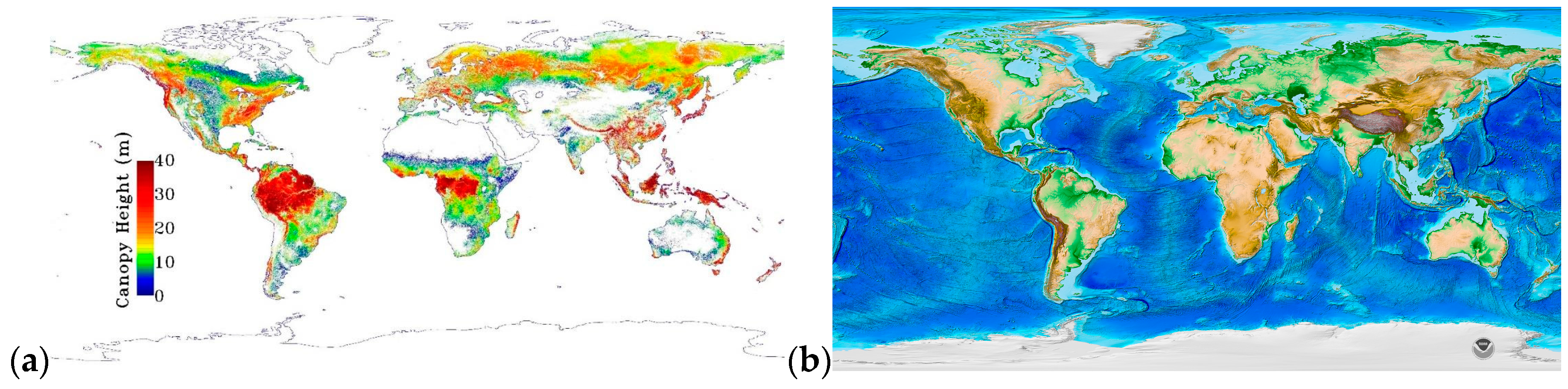Figure 5c shows the good sensitivity of the $\mathrm{PR}$ for different levels of Above Ground Biomass (ABG), from ~100 ton/ha for boreal forests to ~350 ton/ha for tropical rainforests (Figure 7a). The transitions zones from arid to dense vegetation areas are well represented in Africa and Asia from the North to the South. Over dense vegetation areas, the $\mathrm{PR}$ takes negative values, which suggests that the vertical stalks scatter more vertically polarized waves. These maps show that this observable depends on dielectric and scattering property changes over biomass and wetlands (see Amazon river and lakes regions). This is the reason that explains the behaviour in Figure 8a,b where there are two types of waveforms: those with higher power levels corresponding to areas over the Amazon river and riparian forest, and those corresponding only to tropical forests with lower power level because of signal attenuation [11,36]. The attenuation due to vegetation is ${\mathrm{L}}^{\mathrm{canopy}}={\mathrm{e}}^{{\mathsf{\tau }}^{\mathrm{canopy}}/{\cos \mathsf{\theta }}_{\mathrm{inc}}}$, where ${\mathsf{\tau }}^{\mathrm{canopy}}$ is the nadir optical depth of the vegetation layer [11]. Over the Amazon river and riparian forests the $\mathrm{SNR}$ ranges from ~15 dB to ~30 dB depending on the proportions of land signal contamination. The highest power waveforms’ peaks are even stronger than over Greenland because of the specular reflection over smooth and calm water. However, the averaged waveform shows a higher peak power over Greenland than over the Amazon region and a dissymmetric shape (Figure 3). In South America, when the specular point moves away from the tropical forests, the spreading of the waveforms increases, also showing detectability to the Amazon river with a higher $\mathrm{PR}$ value (Figure 5). Furthermore, it is also observed that the spreading of the trailing edge is larger than the leading edge. This aspect over tropical rainforests will be further evaluated at a regional scale.

The topography [11] is a key parameter to take into consideration, in addition to the effects of biomass, because the scattering coefficient ${\mathsf{\sigma }}^0$ is proportional to the probability that a facet could forward scatter the electromagnetic field to the receiver in a specular way. AGB over some areas of the Himalayas is ~200 ton/ha [37], so that both effects (topography and biomass) are merged. 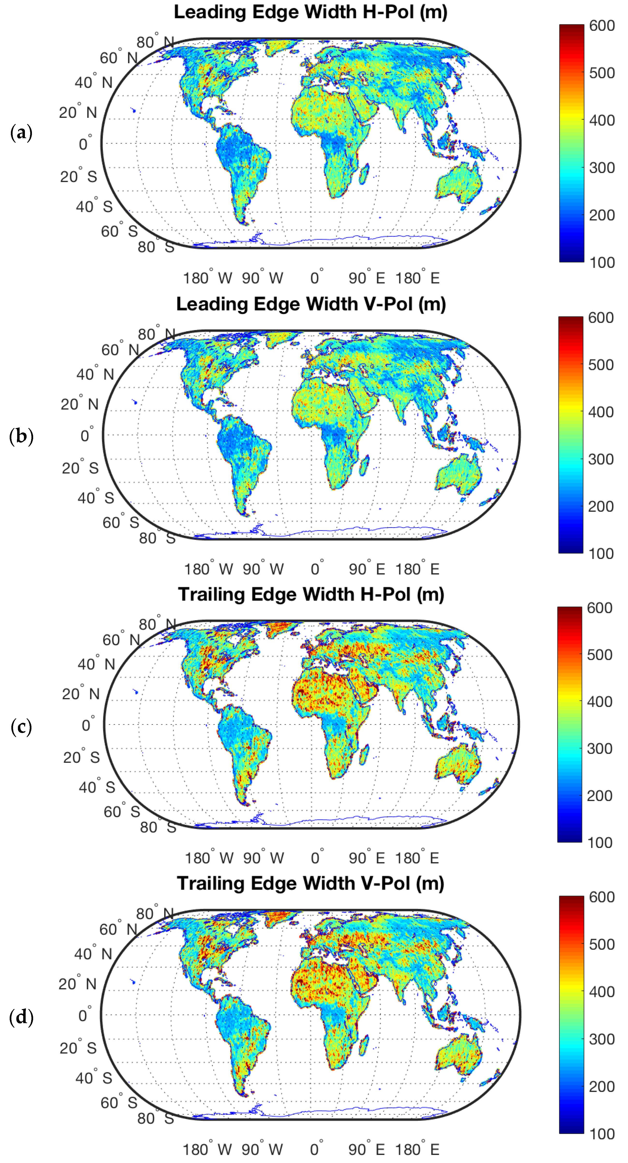Looking at the East mountains of Greenland and the Andes mountains (Figure 7b), neither with appreciable vegetation (Figure 7a), it can be seen that topography contributes to the GNSS signals depolarization (Figure 5c). The effect of topography is further analyzed using the information on the waveforms leading and trailing edges width (Figure 6). Similar measurements of waveform spreading were obtained for H-Pol and V-Pol. At regional scale H-Pol is selected for further study. Similar antenna gain and rate of change of the radar cross-section with the positioning vector, at both polarizations. These observables are used here for the first time (to the authors’ knowledge) for land surfaces applications. In particular, the width of both edges is assessed as a function of the surface type. It is shown that there is a dependence on changes in topography but also in dielectric properties. The width is lower for larger values of biomass and surface topography. This result deserves attention since, in this case, a lower spreading of the waveforms does not mean a higher signal coherence. In the latter case, it means that the area that contributes to the signal in the specular direction is reduced. In the former case, the interpretation is that the effects of attenuation are very strong away from the nominal specular reflection point so that the spreading of the waveform is lower as compared to bare soil.

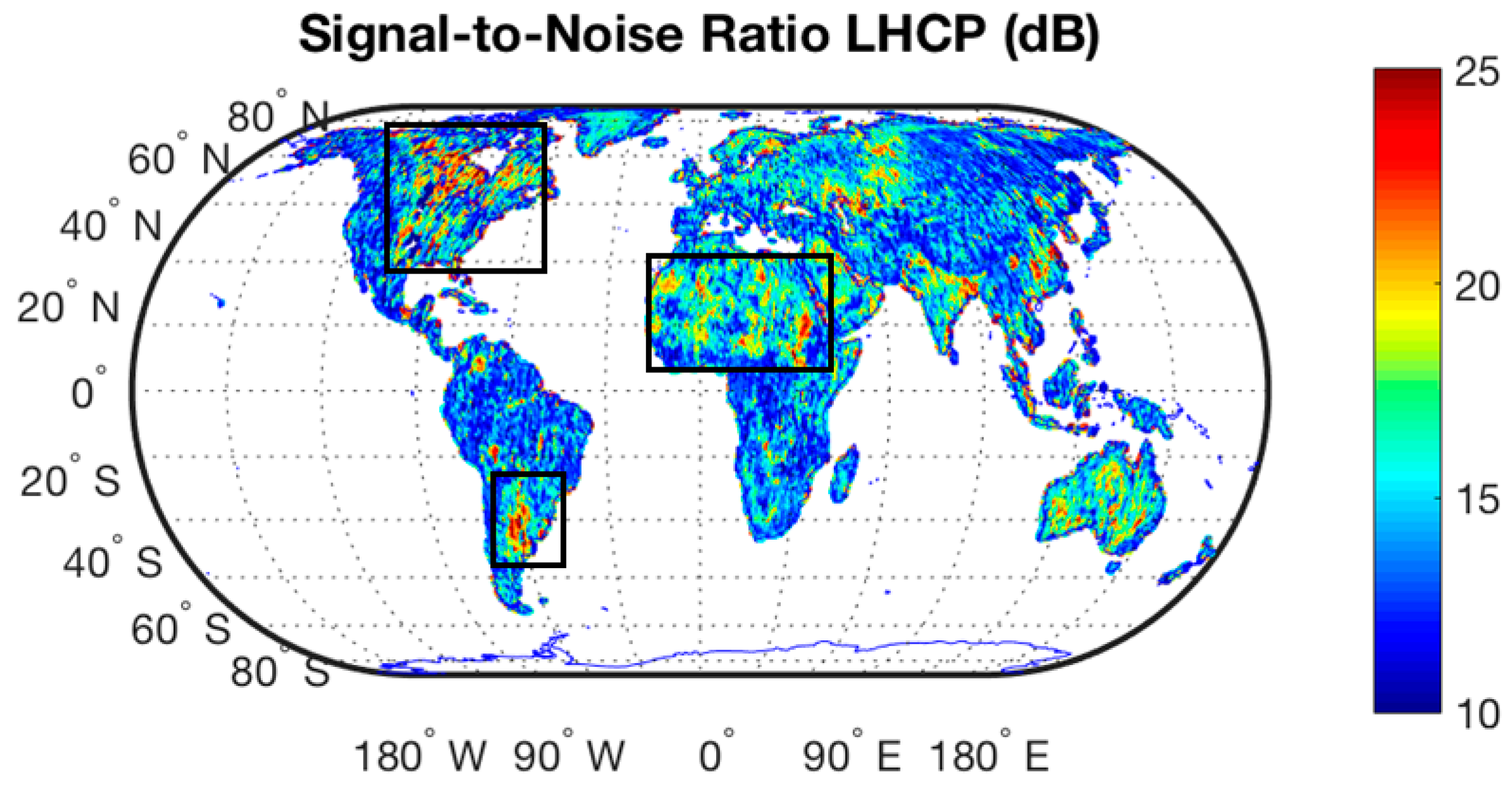
Finally, this reconstructed $\mathrm{SNR}$ at Left Hand Circular Polarization is also shown here for reference (Figure 9) as [32]:

$${\mathrm{SNR}}_{\mathrm{LHCP}}={\left(\frac{\sqrt{{\mathrm{SNR}}_{\mathrm{H}}}+\sqrt{{\mathrm{SNR}}_{\mathrm{V}}}}{2}\right)}^2$$

(12)

Figure 9 shows high peaks power associated with bare regions with high soil moisture values, lakes regions and also over the Sahara Desert (black rectangles in Figure 9). On the other hand, lower power levels are observed over tropical or boreal forests due to the larger signal attenuation.

3.2. Regional Scale

This section provides a regional scale analysis (Figure 10) with focus on Africa-Congolian tropical rainforests, Sahara and Kalahari Desert (Figure 11, Figure 12 and Figure 13), Northern Asia Boreal forests (Figure 14, Figure 15 and Figure 16), and the Greenland ice sheet (Figure 17 and Figure 18). These three regions have been selected because they provide a wide overview of different scattering properties over the Earth’s surface. The information provided by the seasonal variations of the $\mathrm{PR}$, $\mathrm{SNR}$, and the spreading of the waveforms is complemented with maps of Soil Water Index ($\mathrm{SWI}$) from METOP-ASCAT [38], and Normalized Difference Vegetation Index (NDVI) from MODIS [39]. Additionally, the effect of larger AGB on tropical rainforests as compared to boreal forests is derived from the lower levels of $\mathrm{SNR}$ for higher AGB, the lower $\mathrm{PR}$, and the lower spreading of the waveforms, as compared to different terrain types (Figure 10).

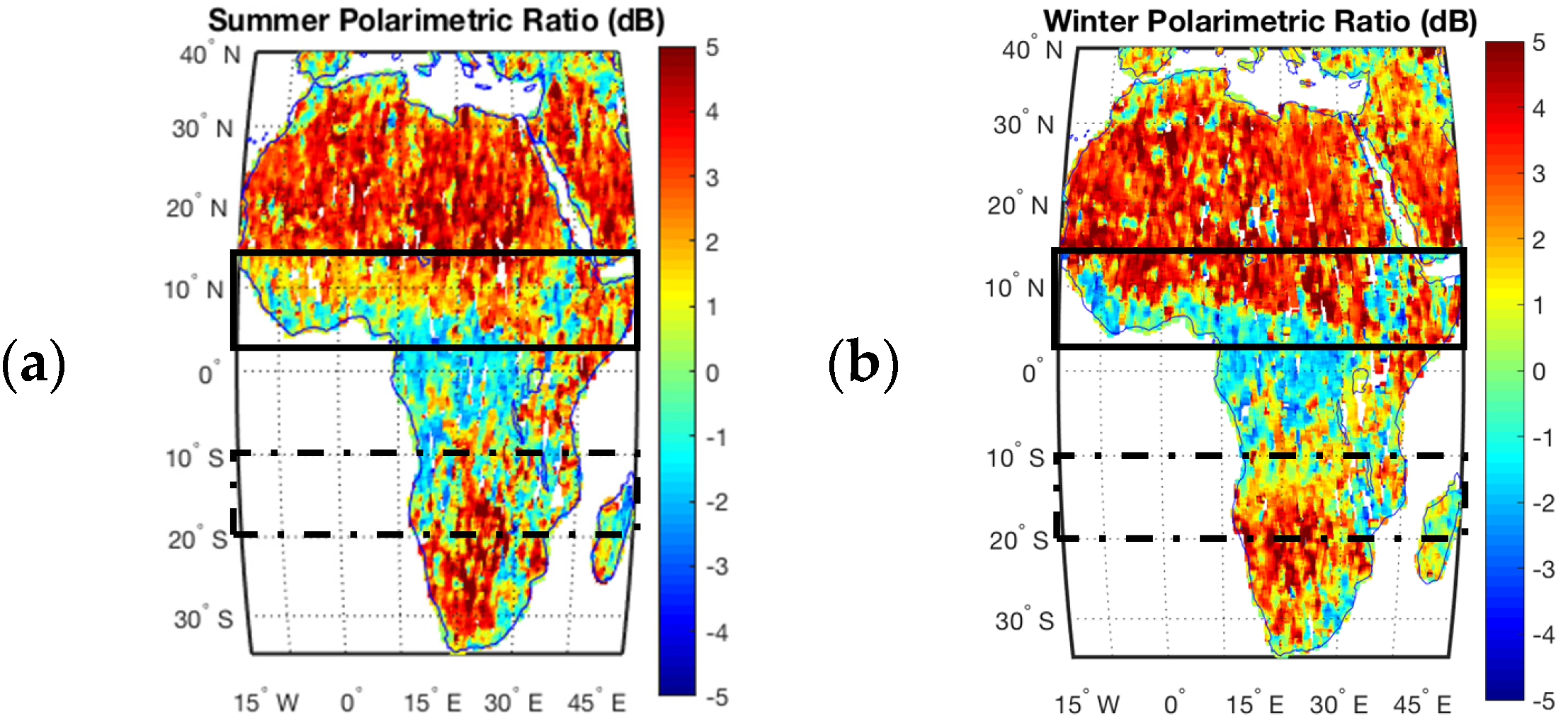
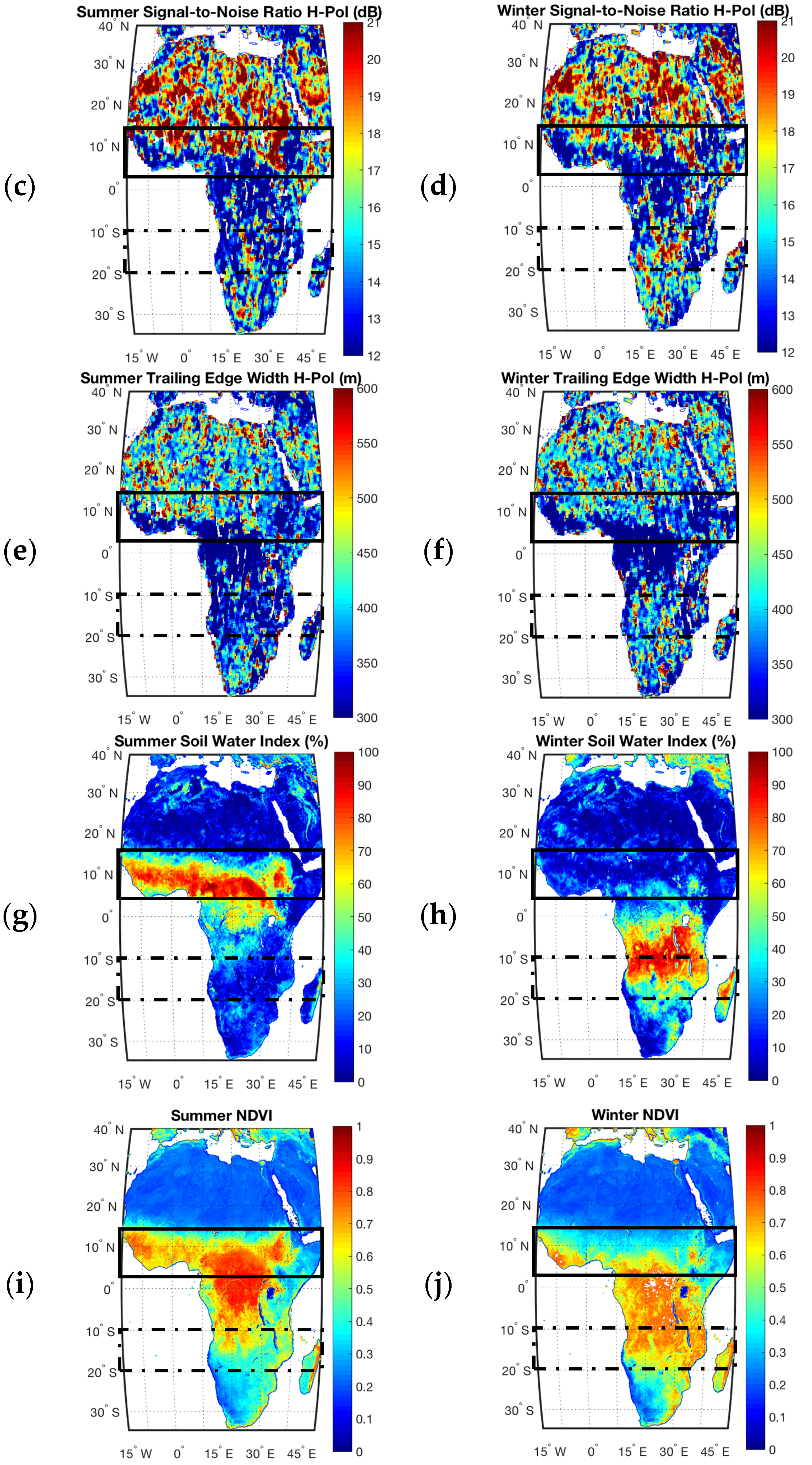
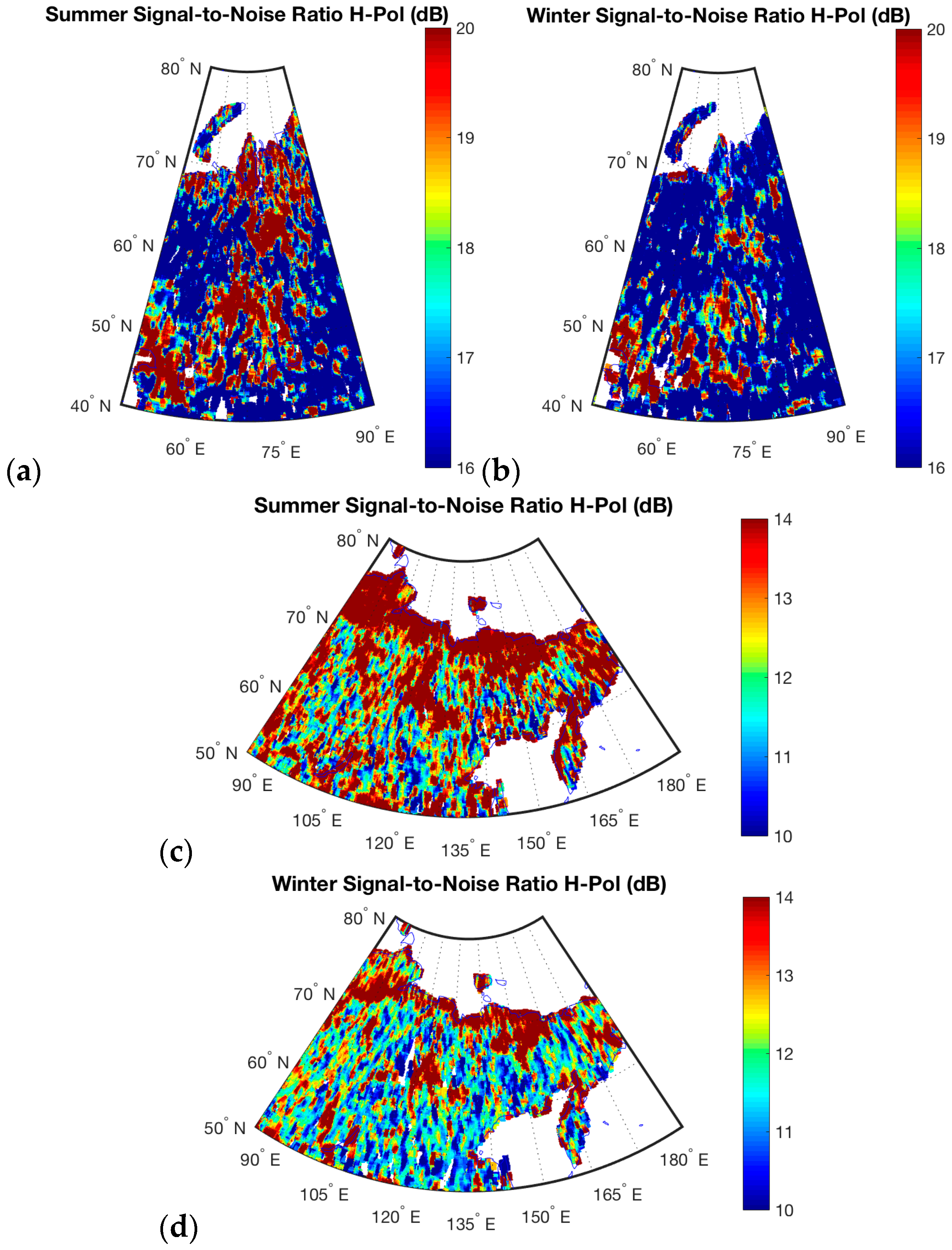
3.2.1. Africa: Arid Deserts and Congolian Rainforests

Over bare soil, the scattering is mainly related to surface scattering, being driven by the soil moisture and surface roughness. However, the high spatial variability of the $\mathrm{SNR}$ over the Sahara Desert could be explained by both surface (Rocky Mountains, boulder and graves zones, and sand seas) and subsurface scattering contributions as Camps suggested for first time in [11]. Volume scattering could occur under dry conditions allowing the GNSS signals to penetrate the subsurface [40,41,42] for rich sand content areas. This could explain the large $\mathrm{SNR}$ values over the Sahara despite the low soil moisture (Figure 11c,d). On the other hand, the large waveform spreading (Figure 11e,f) over the Sahara Desert is difficult to be attributed to this geophysical effect because of the low penetration depth around (~2 m) for 0% of volumetric moisture content at L band. The effect of the sand seas (that continuously reshape the surface) on the scattering coefficient, should be considered as a plausible reason, particularly the dunes, which show the characteristics of the sand and the long-term wind [43]. Additionally, almost negligible seasonal variations over the Sahara are observed since SWI (Figure 10g,h) and NDVI are nearly constant during the year in this region (Figure 11i,j).

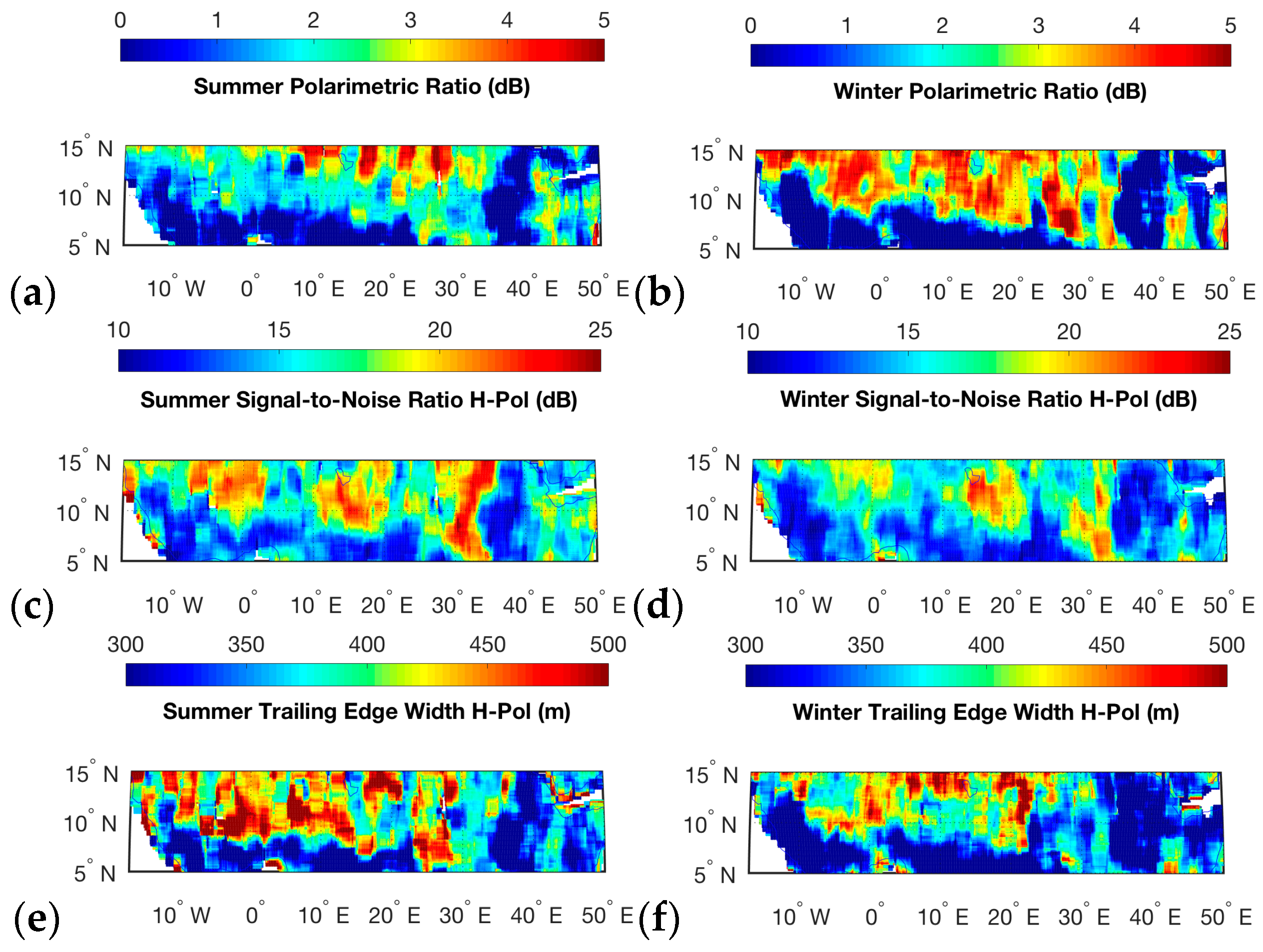
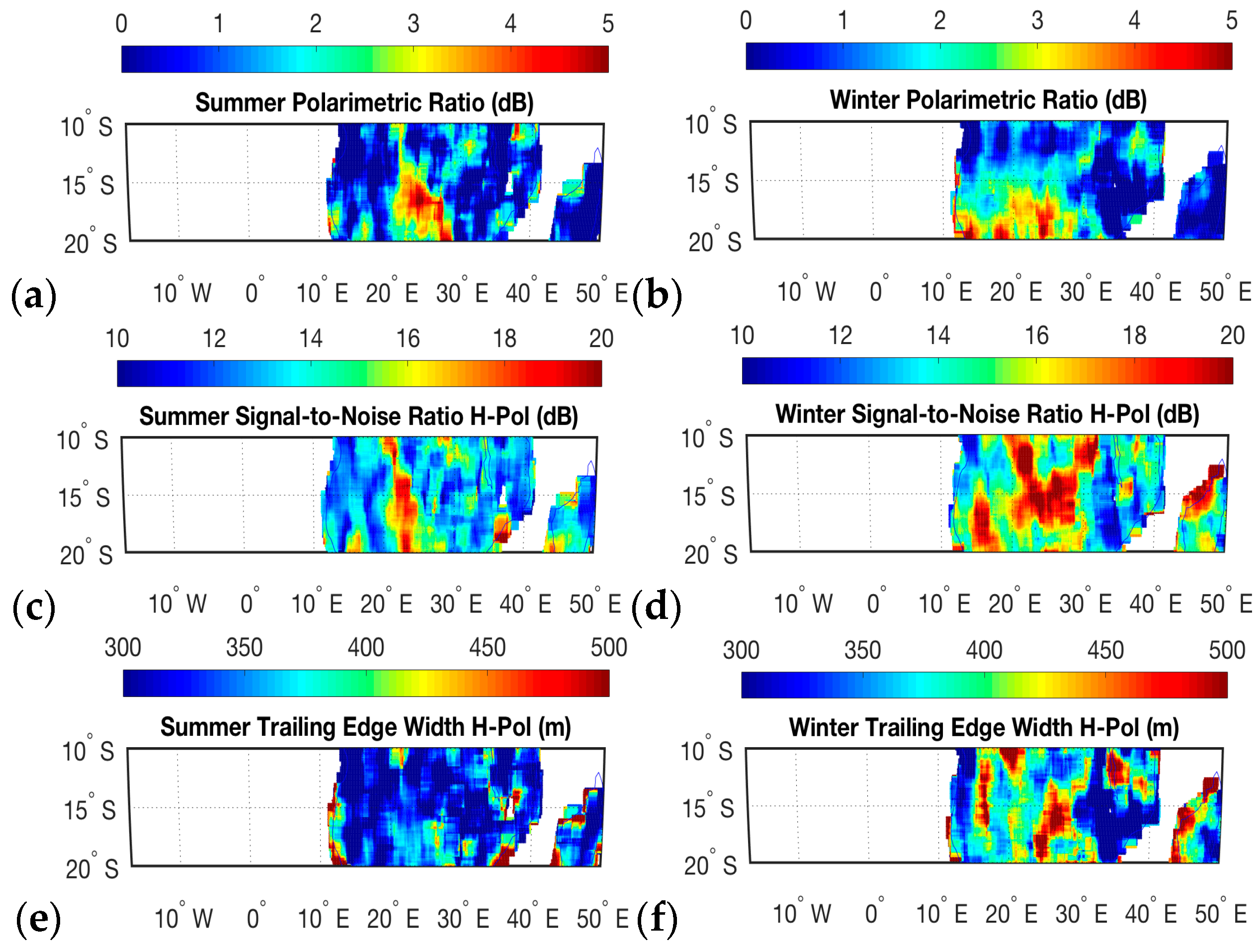
Seasonal fluctuations over Africa are found in the latitude ranges from ~9° to ~15°, and from ~−20° to ~−10°, where the geophysical parameters changes are large from Summer to Winter ($\mathrm{SWI}$ in Figure 11g,h, and NDVI in Figure 11i,j). Seasonal variations of the Polarimetric Ratio (${\mathrm{PR}}_{\mathrm{Summer}}$ ~1 dB in Figure 12a vs. ${\mathrm{PR}}_{\mathrm{Winter}}$ ~4 dB in Figure 12b) are anti-correlated to changes in SWI, and NDVI. On the other hand, seasonal variations at H-Pol in the SNR (${\mathrm{SNR}}_{\mathrm{Summer}}$ ~22 dB in Figure 12c $\&{\mathrm{SNR}}_{\mathrm{Summer}}$ ~13 dB in Figure 13c vs. ${\mathrm{SNR}}_{\mathrm{Winter}}$ ~18 dB in Figure 12d & ${\mathrm{SNR}}_{\mathrm{Winter}}$ ~17 dB in Figure 13d), and the trailing edge width (${\mathrm{TE}}_{\mathrm{Summer}}$ ~460 m in Figure 12e & ${\mathrm{TE}}_{\mathrm{Summer}}$ ~340 m in Figure 13e vs. ${\mathrm{TE}}_{\mathrm{Winter}}$ ~390 m in Figure 12f & ${\mathrm{TE}}_{\mathrm{Winter}}$ ~440 m in Figure 13f) are correlated to changes in $\mathrm{SWI}$ and NDVI. This could be explained since the larger scattering coefficient over the soil, associated with larger $\mathrm{SWI}$, increases the SNR and waveforms spreading, while the larger NDVI attenuates H-Pol signals more than V-Pol signals (Figure 5a,b). The spreading of the waveforms in the latitude range from ~9° to ~15° (Figure 11e,f) is similar to that over the Sahara Desert, with very low levels of NDVI. However, as it is shown over the equatorial region, the spreading is significantly reduced because of the effect of the Congolian forests with an AGB ~350 ton/ha. This suggests that the canopy height (Figure 7a) plays a more important role than the NDVI in the shape of the reflected waveforms. In fact, the $\mathrm{SNR}$ is larger over the Sahara and Kalahari Desert than over Congolian forests despite the larger $\mathrm{SWI}$, because the larger signal attenuation due to the larger AGB (Figure 7a). In regions with lower levels of canopy height, the Polarimetric Ratio is more sensitive to changes in NDVI (Figure 7a, Figure 12a,b, and Figure 13a,b).

3.2.2. Asia: Arid Deserts and Boreal Forests

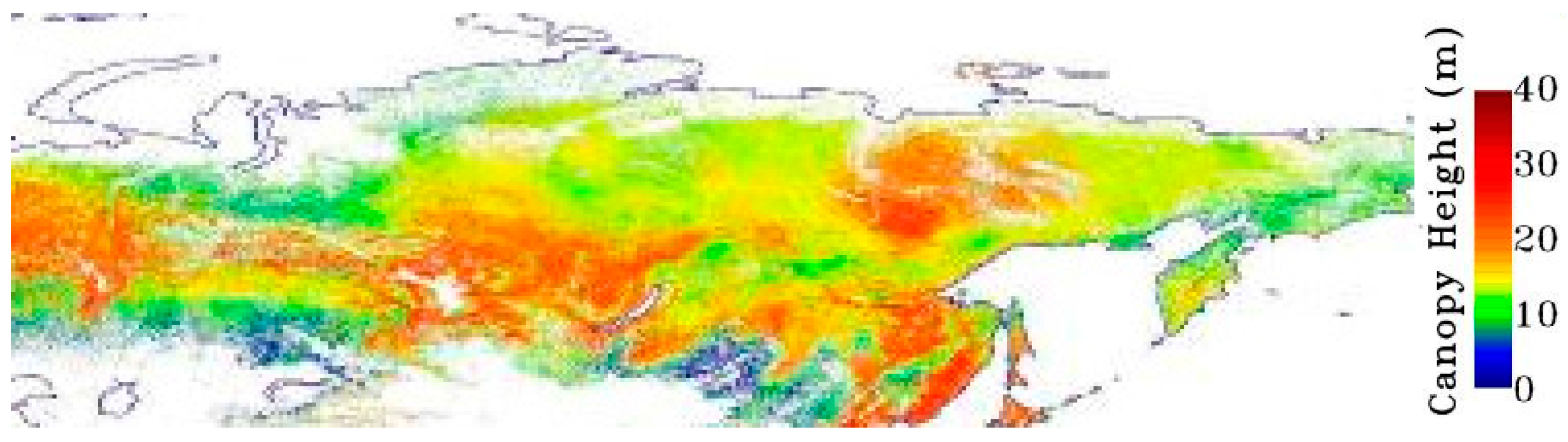
The evaluation over the Northern Asia region is useful to study separately the effects of $\mathrm{SWI}$ and AGB (Figure 14, Figure 15 and Figure 16). The comparison between Figure 14 and Figure 15 shows the effects of higher AGB on the waveforms’ parameters, for relatively homogeneous SWI conditions at latitudes higher than ~ 55° (Figure 15g). SWI data from ASCAT could have some limitations for high vegetation density because measurements are derived using a radar operating at a high frequency ~5.2 GHz (C-band). The trailing edge width is lower (Figure 15e,f) over regions with higher canopy height (Figure 14), and rapidly increases over the Gobi Desert or over the highest latitudes in Siberia. On the other hand, the highest $\mathrm{PR}$ values (Figure 15a,b) and $\mathrm{SNR}$ values (Figure 15c,d) are associated to regions with larger values of the trailing edge width (Figure 15e,f). As is shown in Figure 15g−j, NDVI is not associated with $\mathrm{SWI}$ over Northern Asia in Winter or Summer. Canopy height (Figure 14) is a key parameter. The spreading of the waveforms, the $\mathrm{PR}$, and $\mathrm{SNR}$ values show approximately a similar trend in Summer (Figure 15a,c,e) and Winter (Figure 15b,d,f), but different absolute values. The main difference is the smaller waveforms’ spreading in areas with higher values of AGB. Additionally, the $\mathrm{SNR}$ is lower in Winter (Figure 16), particularly over areas with lower AGB values, because of the effect of snow on the surface at these latitudes. This additional signal attenuation explains the lower spreading of the signals in Winter, since a smaller region around the nominal specular point contributes to the power waveforms. Finally, it is found that $\mathrm{PR}$ is lower in Summer over Northern Siberia (in agreement with Figure 12) because of the high soil moisture level in Summer (Figure 15g) and snow conditions in Winter (Figure 15h).

3.2.3. North America and Greenland: Lakes Region and Ice Cap

GNSS-R applications can be extended to the study of snow and ice [44,45,46]. The signal wavelength (λ) at L2 is λ ~24 cm, which is much longer than that radiometers operating at different frequency bands such as AMSR-E and AMSR-2. The wavelength is larger than the grain size and even the snowpack thickness. As a consequence, the medium can be assumed to be homogeneous so that the scattering is determined by the local density fluctuations. At this frequency, ice has a very low absorption coefficient and the refractive index is small. The penetration depth and the scattering coefficient depend on frequency and snow properties. In the case of dry snow, the penetration depth is expected to be around hundreds of meters and therefore the GNSS-R technique is potentially optimum for subsurface studies [47]. On the other hand, the penetration depth of GNSS signals over sea ice is <1 m [48].

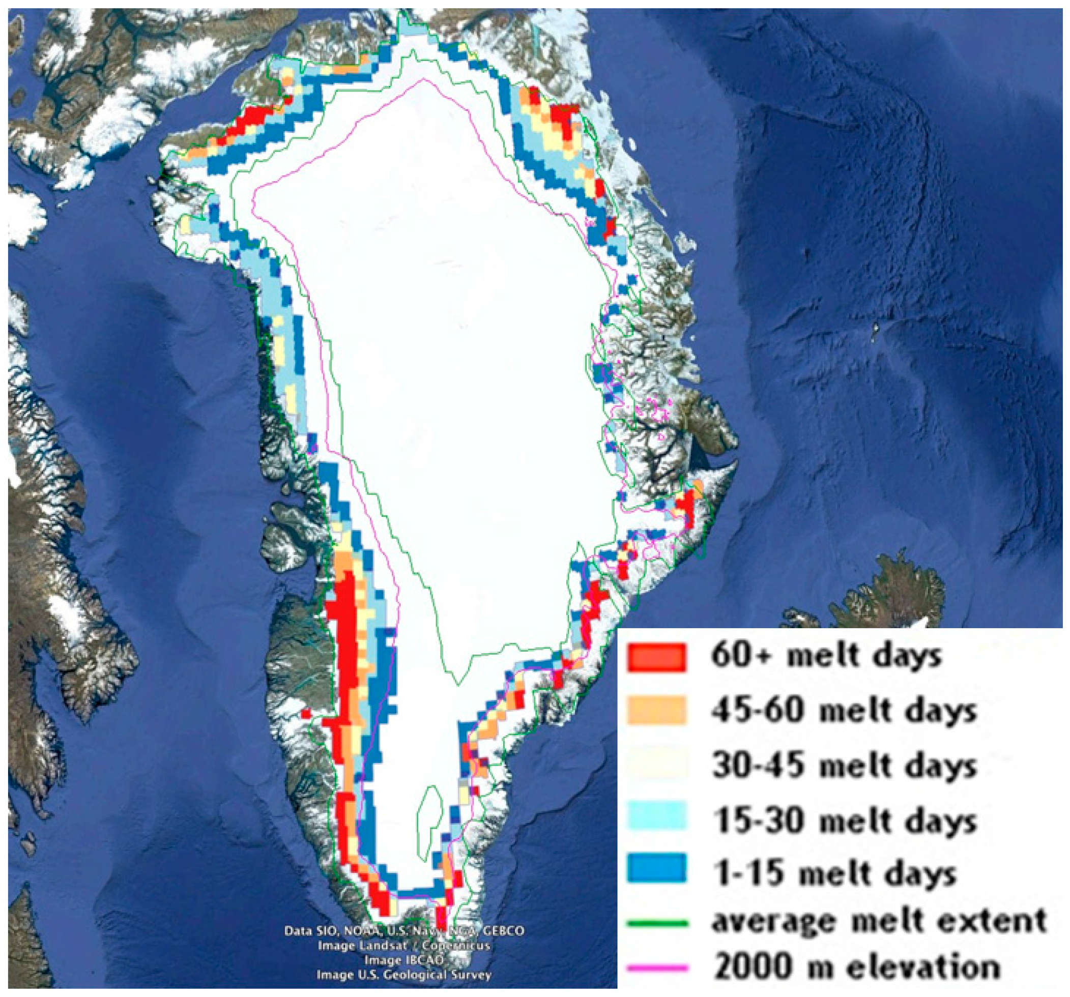
Extended regions of Antarctica and Greenland are affected by melting effects (e.g., Figure 17). A recent study [49] additionally shows areas alternatively frozen and thawed in Greenland’s inner ice cap (magenta line in Figure 17). Greenland is a focus region of this study (Figure 18). Firstly, it is noted that over bare soil the scattering is significantly determined by soil moisture and surface roughness. However, over dry ice, volume scattering [50], and scattering at different layers [44] could occur allowing the GNSS signals to penetrate the subsurface. The larger waveform spreading over Greenland (Figure 18e,f) could be attributed to this geophysical reason. The effect of subsurface scattering is to increase the waveforms’ peak power (Figure 18c,d) and the signals’ spreading [50], in agreement with Figure 3e,f. At the same time, in the frame of this work, the large SMAP’s antenna gain ~36 dB partially compensates the signal attenuation. Therefore, the sensitivity to penetrating signals as seen by SMAP is large as compared to satellites with smaller antennas. Figure 18 shows high values of $\mathrm{SNR}$ ~ (18, 22) dB, $\mathrm{PR}$ ~ (3, 5) dB, and trailing edge width ~ (500, 600) m over areas in the inner ice cap. However, the waveforms parameters ($\mathrm{SNR}$, $\mathrm{PR},$ and trailing edge) take alternatively low and high values over these areas. On the other hand, the parameters levels are qualitatively similar to those over outer Greenland (see melting effects in Figure 17). Additionally, the width of the waveforms’ trailing edge over Greenland increases from Summer (Figure 10 and Figure 18e) to Winter (Figure 10 and Figure 18f) when the weather is colder and the amount of dry ice increases, and therefore the penetration depth would be larger. This waveform data is consistent with the waveforms spreading being due to subsurface scattering effects.

Over North America, it is found that during Summer there are regions with high $\mathrm{SNR}$ values corresponding to areas with lakes and high SWI (Figure 18g). During Winter, these power peaks are lower because of the effect of snow over the surface that reduces the scattering coefficient.

4. Final Discussion

A serendipitous GNSS-R experiment performed with the SMAP radar receiver has provided a rather unique data set. The use of the Polarimetric Ratio ($\mathrm{PR}$) at H-Pol and V-Pol from a GNSS-R spaceborne mission has been evaluated for the first time. This work provides an advance in the understanding of GNSS-R scatterometry over land surfaces and cryosphere enabled by the high gain of the radar antenna (~36 dB) and the use of two orthogonal polarizations. Additionally, the second added value of this work is the analysis of waveform spreading due to the scattering process over the Earth’s surface, showing the ability to detect different levels of AGB over Amazonian and Boreal forests, differentiating from deserts and the cryosphere. Values of soil moisture as provided by the SMAP’s radiometer, and SWI and NDVI maps have been used here to help in the interpretation of the GNSS-R observables. It is found that despite the good correlation between $\mathrm{PR}$ and the soil moisture values, the GNSS-R signatures simultaneously contain information about AGB, soil moisture, and topography, making it difficult to separate the contributions. These issues need to be addressed to potentially provide accurate soil moisture measurements (key-factor for studies of the water cycle that is a continuous sequence involving water in the atmosphere, on the continents, and in the ocean), and biomass measurements (key-factor for evaluation of the carbon cycle).

5. Conclusions and Future Opportunities

A GNSS-R experiment has been performed from the NASA’s SMAP satellite after tuning the radar receiver to the GPS L2 frequency (1227.6 MHz). Delay Doppler Maps (DDMs) were computed on-ground using a clean-replica of the open-access L2C code. Upon investigation, it was determined that the optimum coherent integration time for this experiment was ${\mathrm{T}}_{\mathrm{coh}}$ = 5 ms. The high gain of the SMAP’s antenna allowed it to receive strong signals from a variety of scenes. First results have been presented to investigate the characteristics of the reflected waveforms over land surfaces and cryosphere. The main observations from this study are: (a) the Polarimetric Ratio ($\mathrm{PR}$) provided by this data set and the soil moisture content provided by the SMAP’s radiometer show a Pearson linear correlation factor $\mathrm{r}$ ~ −0.6; (b) the Signal-to-Noise at H-Pol (${\mathrm{SNR}}_{\mathrm{H}}$) shows different mean levels for different terrain types: ${\mathrm{SNR}}_{\mathrm{H},\mathrm{Lakes}}$ ~ 25 dB, ${\mathrm{SNR}}_{\mathrm{H},\mathrm{Sahara}}$ ~ 18 dB, ${\mathrm{SNR}}_{\mathrm{H},\mathrm{Greenland}}$ = 17 dB, ${\mathrm{SNR}}_{\mathrm{H},\mathrm{Boreal}\mathrm{Forests}}$ ~ 13 dB, ${\mathrm{SNR}}_{\mathrm{H},\mathrm{Tropical}\mathrm{Forests}}$ ~ 12 dB; (c) the waveforms’ parameters show sensitivity to seasonal fluctuations over regions with seasonal changes of geophysical parameters expressed by NDVI, and SWI; (d) the spreading of the waveforms’ leading and trailing edge reduces for higher values of AGB (from ${\mathrm{ABG}}_{\mathrm{Boreal}}$ ~100 ton/ha to ${\mathrm{AGB}}_{\mathrm{Tropical}}$ ~350 ton/ha); (e) the AGB shows a more pronounced effect in GNSS-R signatures ($\mathrm{PR}$, $\mathrm{SNR}$, leading & trailing edges width) than NDVI; (f) the GNSS signals are depolarized upon scattering over areas with rough topography or high levels of AGB; and (g) the large spreading of the waveforms over the Greenland’s ice cap suggests that the GNSS signals penetrate the subsurface significantly, which opens the possibility of cryosphere monitoring using GNSS-R sensors from space.

While the GNSS-R experiment on SMAP was helpful in providing high $\mathrm{SNR}$ polarimetric data, the sampling characteristics are not optimal for process studies. On the other hand, the unprecedented improved spatio-temporal sampling provided by the NASA’s CyGNSS suggests the possibility to use its data to study soil moisture and vegetation water content variability in the tropical latitudinal bands. A careful assessment should be performed of the potential synergies between CyGNSS and SMAP GNSS-R data sets to evaluate how the SMAP’s high $\mathrm{SNR}$ polarimetric data could help elucidate some of the scattering mechanisms not observable with the CyGNSS lower antenna gain.