A Novel Statistical Approach for Ocean Colour Estimation of Inherent Optical Properties and Cyanobacteria Abundance in Optically Complex Waters

Abstract

Eutrophication is an increasing problem in coastal waters of the Baltic Sea. Moreover, algal blooms, which occur every summer in the Gulf of Gdansk can deleteriously impact human health, the aquatic environment, and economically important fisheries, tourism, and recreation industries. Traditional laboratory-based techniques for water monitoring are expensive and time consuming, which usually results in limited numbers of observations and discontinuity in space and time. The use of hyperspectral radiometers for coastal water observation provides the potential for more detailed remote optical monitoring. A statistical approach to develop local models for the estimation of optically significant components from in situ measured hyperspectral remote sensing reflectance in case 2 waters is presented in this study. The models, which are based on empirical orthogonal function (EOF) analysis and stepwise multilinear regression, allow for the estimation of parameters strongly correlated with phytoplankton (pigment concentration, absorption coefficient) and coloured detrital matter abundance (absorption coefficient) directly from reflectance spectra measured in situ. Chlorophyll a concentration, which is commonly used as a proxy for phytoplankton biomass, was retrieved with low error (median percent difference, MPD = 17%, root mean square error RMSE = 0.14 in log₁₀ space) and showed a high correlation with chlorophyll a measured in situ (R = 0.84). Furthermore, phycocyanin and phycoerythrin, both characteristic pigments for cyanobacteria species, were also retrieved reliably from reflectance with MPD = 23%, RMSE = 0.23, R² = 0.77 and MPD = 24%, RMSE = 0.15, R² = 0.74, respectively. The EOF technique proved to be accurate in the derivation of the absorption spectra of phytoplankton and coloured detrital matter (CDM), with R² (λ) above 0.83 and RMSE around 0.10. The approach was also applied to satellite multispectral remote sensing reflectance data, thus allowing for improved temporal and spatial resolution compared with the in situ measurements. The EOF method tested on simulated Medium Resolution Imaging Spectrometer (MERIS) or Ocean and Land Colour Instrument (OLCI) data resulted in RMSE = 0.16 for chl-a and RMSE = 0.29 for phycocyanin. The presented methods, applied to both in situ and satellite data, provide a powerful tool for coastal monitoring and management.

1. Introduction

Phytoplankton and coloured detrital matter (CDM), which includes yellow substances (CDOM) and detritus, play an important role in global carbon cycling and climate, e.g., [1,2,3,4]. Phytoplankton are primary producers, which regulate the photosynthetic efficiency of carbon fixation [5,6,7], transfer primary production to higher trophic levels, e.g., [8], and export carbon to the deep oceans, e.g., [3,9,10]. CDM is an optically significant component that strongly absorbs light in the blue and ultraviolet range of the spectrum. It impacts photochemical processes [1,11] and influences phytoplankton and bacterial productivity [12]. Moreover, CDM characterises an accumulation of dissolved organic carbon [1,13]. Reliable information about the dynamics of phytoplankton and CDM in ocean waters gives a better understanding of the role of the ocean in the global carbon cycles.

Optically significant components of the water column can be derived from ocean colour and can be used as indicators of water quality (e.g., level of eutrophication, presence of phytoplankton blooms). Absorption spectra and pigment composition can be used as proxies to characterise the abundance and composition of phytoplankton and CDM. Large blooms of filamentous cyanobacteria form every summer in the waters of the Baltic Sea, and consist mainly of the species Nodularia spumigena, Aphanizomenon flos-aquae, and Dolichospermum sp. These organisms may contain hepato- and/or neurotoxins and can seriously impact human and ecosystem health, the fisheries, and tourism and recreation economies. For these reasons, remote monitoring of optical properties in the Baltic Sea has become increasingly used tool [14,15]. For example, the user-friendly monitoring system of the Baltic environment developed by a Polish research team within the ‘SatBaltic’ project [16,17] that provides maps of hydrodynamic and bio-optical properties in the Baltic Sea.

Phytoplankton pigments act as indicators of phytoplankton composition and biomass in ocean waters [18]. Laboratory methods used to quantify pigments, such as high-performance liquid chromatography (HPLC) or spectroscopy of solvent extracts are accurate but time and labour consuming. Therefore, there is a need for remote sensing algorithms to rapidly estimate phytoplankton pigments over large geographic areas. Indeed, algorithms for estimating chlorophyll a, a primary photosynthetic pigment have been studied for decades [19,20,21,22,23]. Some pigments that occur in particular phytoplankton groups or taxa have been recognised as signatures for those groups or taxa, and their concentrations are used as indicators for the presence of these organisms in the water column [2,24,25,26]. The summertime blooms of filamentous cyanobacteria in the Baltic Sea are known to contain large quantities of phycocyanin that may provide a more specific indicator of cyanobacterial biomass than chlorophyll a, which is present in all phytoplankton species [27,28]. Phycocyanin absorbs light strongly around 620 nm [29], allowing for its quantification from remotely sensed data [28,30,31]. Additionally, Baltic Sea waters are characterised by the high abundance of picoplankton Synechococcus sp. This species may contribute up to 50% of the total phytoplankton biomass during summer and is rich in phycoerythrin [32]. Moreover, the pigment system of cyanobacteria produces a relatively weak chlorophyll a fluorescence signal, whereas the fluorescence yield of phycobilin pigments is comparatively high, carrying a significant amount of spectral information that can be used to assess the abundance of cyanobacteria by means of remote sensing [33,34]. The optical properties of the Baltic Sea are very strongly influenced by high concentrations of coloured dissolved organic material (CDOM) [35] and detrital material [36], which is known to confound existing ocean colour algorithms, especially band ratio approaches for estimating chlorophyll a concentration (chl-a) [21,22,37,38,39]. As the above points suggest, developing ocean colour algorithms to accurately estimate pigment concentrations in the optically-complex waters of the Baltic Sea is not a trivial task. Moreover, the optical properties of different Baltic Sea basins vary widely, so local algorithms are needed.

In this study we use an empirical orthogonal function (EOF) approach that has previously demonstrated its efficacy [3,40,41,42] as an alternative to known ‘band ratio’ algorithms. EOF analysis (also known as a principal component analysis) is a powerful technique for data dimension reduction [43]. EOFs are ordered by decreasing eigenvalue so that, among the EOFs, the first mode, having the largest eigenvalue, accounts for most of the variance of the data [44]. New variables can be constructed by projecting the original dataset onto individual EOFs. Elements of these new variables (scores) result from linear combinations of the variables in each original dataset record weighted according to the EOF elements (loadings). By using the EOFs that account for the most variance, the dimensionality of the original dataset can be reduced while retaining its primary information. Thus, very few empirical modes can generally be used to describe the variability in a very large data set. EOF analysis has been used in many physical and optical research studies, e.g., [44,45], to show temporal and spatial patterns.

Craig et al. [41] showed that EOF analysis of remote sensing reflectance (R_rs) spectra could be used to derive accurate models for estimating water constituents. They showed that EOF analysis of R_rs (λ) spectra revealed information on the factors driving R_rs (λ) variability, and that these could be used as a predictor of variables in multiple linear regressions. Studying the optical properties of the Gulf of Gdansk, we hypothesised that the EOF approach would allow us to derive accurate metrics of pigment concentration and absorption spectra. The EOF method has been shown to accurately estimate the abundance of phycoerythrin in several different water types [46,47]. Additionally, the method performs very well in optically complex waters even when CDOM dominates the absorption signal [41], further suggesting its suitability for our purposes.

The aim of this paper is to use in situ hyperspectral reflectance R_rs (λ) combined with field data collected from the Gulf of Gdansk to quantify parameters that are water quality indicators. Local remote sensing algorithms were developed to derive CDM and phytoplankton absorption coefficients as well as the phytoplankton pigment concentration in the optically complex water of the Gulf of Gdansk. Additionally, the method was adapted for multispectral satellite radiometers to retrieve the concentration of chlorophyll a and the cyanobacteria marker pigment (phycocyanin), typical for the region. This allows for improved spatial and temporal resolution in the monitoring of cyanobacteria blooms.

Table 1. List of symbols, definitions, and units.

Symbol	Description	Unit
CDOM	Coloured Dissolved Organic Matter
CDM	Coloured Detrital Matter
aCDOM	CDOM absorption coefficient	m−1
aCDM	CDM absorption coefficient	m−1
aph	Phytoplankton absorption coefficient	m−1
adet	Nonalgal particles absorption coefficient	m−1
chl˗a	Chlorophyll a concentration	mg·m−3
Ed	Downwelling irradiance	W·m−2·nm−1
Lu	Upwelling radiance	W·m−2·nm−1·sr−1
PC	Phycocyanin concentration	mg·m−3
PE	Phycoerythrin concentration	mg·m−3
Rrs	Remote sensing reflectance	sr−1
˂Rrs˃	Integral˗normalised remote sensing reflectance	dimensionless

lists all optical properties and variables used in this study.

2. Material and Methods

2.1. In Situ Measurements

All measurements were performed as part of the Satellite Monitoring of the Baltic Sea environment Project No. POIG.01.01.02-22-011/09, ‘SatBaltic’ [16,17]. Data were collected during field campaigns in late spring and summer in 2012 and 2013 in the Gulf of Gdansk (Baltic Sea). Measurements were taken at 6 locations in the area between 18.4–20°E and 54.2–54.8°N (Figure 1). Cruises took place twice per month in May and September, and 4 times per month in June, July, and August, when the likelihood of phytoplankton blooms is the highest. In total, more than 80 data sets were gathered. The Gulf of Gdansk, in the southern Baltic Sea, belongs to optical case 2 waters [48] dominated by coloured dissolved organic matter (CDOM) [14,35], and by suspended particulate matter in coastal areas [14]. The Gulf of Gdansk is a wide and relatively shallow water body, connected to the open sea and strongly influenced by riverine waters. It has many different hydro-geomorphological regimes including lagoons, river mouths, sheltered and open coastal areas, and is subject to strong anthropogenic pressure [49].

2.1.1. Water Sample Acquisition and Analyses

Particulate and phytoplankton absorption spectra were determined from water samples filtered under low pressure immediately after sampling using 25 mm Whatman GF/F glass-fibre filters. The spectra of the particulate material collected on the filters were measured between 400–800 nm using a Perkin Elmer Lambda 850 dual-beam spectrophotometer equipped with a 15 cm Labsphere integrating sphere. Total particulate absorption (a_p; m⁻¹) was measured by placing the filter in the centre of the integrating sphere using a special filter holder (c.f. Röttgers and Gehnke [50], and a 25 mm GF/F filter saturated with 0.2 μm filtered sea water was used as a blank). The particulate matter was then de-pigmented using a solution of NaClO [51], and the non-algal particle absorption (a_det; m⁻¹) was measured in the same way as described above. The phytoplankton absorption spectra were then calculated as the difference between the particle and nonalgal particle absorption. The obtained values in the near-infrared part of the spectrum (>750 nm) oscillated around zero, and therefore no zero-point correction was needed. The values of the absorption coefficient were calculated using the formula proposed by Wojtasiewicz et al. [52] for samples containing cyanobacteria species.

Absorption by coloured dissolved organic matter (a_CDOM; m⁻¹) was determined by first filtering seawater samples through Millipore 0.2 µm membrane filters. The filtrate was kept refrigerated in amber glass bottles until analysis. The absorption spectra of the samples were then measured using a Perkin Elmer Lambda 850 dual-beam spectrophotometer, with milliQ water used as a blank. The path length of the cuvette (10, 5, or 1 cm) was chosen based on the CDOM concentration.

Chlorophyll a concentration (chl-a; mg·m⁻³) was determined according to Baltic Monitoring Protocol [53]. The samples were filtered through Whatman GF/F filters which were kept frozen at −80 °C until analysis. Using 96% ethanol, the phytoplankton pigments were then extracted for 24 h in the dark from the material retained on the filters. The samples were then centrifuged for 15 min at 4000 rpm and the supernatant pipetted into a 1 cm cuvette. The absorbance spectra of the extracts were measured in the spectrophotometer against 96% ethanol as a blank. The chl-a was calculated using the following formula:

$$\mathrm{chl}-a=\frac{{10}^3(O{D}_{665}-O{D}_{750})\cdot V_{extr}}{83\cdot V_f\cdot l}$$

(1)

where OD₆₆₅ is the optical density at 665 nm, OD₇₅₀ is the optical density at 750 nm, V_extr is the volume of ethanol used for the extraction (cm³), V_f is the volume of filtered sample (dm³), al is the length of the cuvette (cm), and the number 83 is optical density of chlorophyll a in the 96% ethanol.

The samples for determination of phycobilin concentrations were collected and stored in the same way as the chlorophyll samples. Phycobilins were extracted from the cells using the extraction medium consisting of 0.25 M Trizma Base, hydrated 10 mM disodium EDTA (2 H₂O), and 2 mg·cm⁻³ lysozyme, with initial pH 9 adjusted to a final pH 5.5 (HCl) according to Steward and Farmer [54] in darkened room conditions. In order to improve the extraction efficiency the cells were disintegrated by combining gentle mechanical grinding and enzymatic reaction. Then the optical densities of the extracts at 620 nm were used to calculate the PC concentration according to Sobiechowska-Sasim et al. [34].

Additionally, the taxonomic composition of the phytoplankton community was determined in the Regional Centre of Cyanobacteria (University of Gdansk) using microscopic examination [53].

2.1.2. Radiometry Measurements and Analysis

Downwelling irradiance above the water (E_d (0⁺,λ); W·m⁻²·nm⁻¹) and upwelling radiance just below the water surface (L_u (0⁻,λ); W·m⁻²·nm⁻¹·sr⁻¹) were measured using a RAMSES TriOS hyperspectral RAMSES−ACC−VIS irradiance and RAMSES−MRC radiance sensors. The sensors measured the signal in 190 channels within the range of 320 nm to 950 nm with a spectral sampling of 3.3 nm and a spectral accuracy of 0.3 nm. The radiance radiometer is characterised by a narrow detector and a nominal full-angle field of view of 20° in air which helps to minimise self-shading during measurements. The radiometer was mounted on a float to obtain measurements just below the water surface (around 3 cm depth). In order to calculate the remote sensing reflectance (R_rs; sr⁻¹), the upwelling radiance measured below the water surface L_u (0⁻,λ) was propagated through the air-sea interface by applying the immersion factor I_f [55,56]. R_rs (0⁺,λ) was then calculated with the following equation:

$$R_{\mathrm{rs}}(0^{+},\lambda )=\frac{L_{\mathrm{u}}(0^{+},\lambda )}{E_{\mathrm{d}}(0^{+},\lambda )}$$

(2)

2.1.3. Synthetic Satellite Remote Sensing Reflectance

While hyperspectral radiometers are becoming increasingly popular for field measurements, many satellite missions utilise multispectral radiometers (e.g., MODIS–Aqua (NASA), MERIS (Envisat), OLCI (Sentinel-3)). To explore the feasibility of implementing our models for multispectral satellite data, a synthetic satellite dataset (R_rs^sat) was created following [41]. The synthetic data were created from the in situ measurements of hyperspectral R_rs by averaging the data around the waveband centres used on the MERIS and OLCI radiometer between 400 and 800 nm: 412.5, 442.5, 490, 510, 560, 620, 665, 681.25, 708.75, 753.75, 761.25, and 778.75 [57]. A Gaussian curve was defined with a full width half maximum (FWHM) of the corresponding bandwidths and this was used to weight R_rs values on either side of the band centre during averaging.

2.2. Statistical Methods

2.2.1. Empirical Orthogonal Function Approach and Stepwise Fitting Procedure

Following the method described in Craig et al. [41], empirical orthogonal function (EOF) analysis was performed on the R_rs spectra. The EOF method utilises variability in spectral shape rather than in magnitude of the R_rs spectra to make predictions. Measured spectra were therefore integral normalised using the following equation:

$$<R_{rs}>=\frac{R_{rs}}{{\displaystyle {\int }_{400}^{800}{R}_{rs}d\lambda }}$$

(3)

Normalised spectra are decomposed into EOF or modes that can be used as variables in a multilinear regression (4). The regression has the following form:

$${\log }_{10}(\mathrm{Y})=k+{\displaystyle \sum _{\mathrm{m}=1}^M{l}_{\mathrm{m}}\cdot {\log }_{10}\left(X_{\mathrm{m}}\right)}$$

(4)

where Y is the dependent variable, M is the number of EOFs selected (see next paragraph), X_m are the scores of the selected EOF modes, and k and l_m are regression coefficients.

Our methodology differed from that described by Craig et al. [41] in one important aspect; instead of using the first few modes as regression variables, we employed stepwise regression to objectively chosen set of modes for inclusion in the model [42,47]. Stepwise regression is a systematic method for adding and removing independent variables (i.e., the modes in our analysis) in a multilinear model based on their statistical significance. The method begins with an initial model and then compares the explanatory power of incrementally larger and smaller models. At each step, the p-value of an F-statistic is computed to test models with and without a potential mode. Although a mode may explain only a minute portion of the total variance in R_rs, it may still be a statistically significant predictor of the dependent variable.

The modes produced by the EOF analysis capture systematic variations in spectral shape. It is possible that some of these modes represent instrument noise with no relation to a biological process. To eliminate such modes, a signal-to-noise criterion was applied. First, each mode was smoothed using a Savitzky-Golay filter. The resulting spectral shapes were considered the signal, and the difference between the original and filtered mode was considered noise. The signal to noise ratio (SNR) was calculated for each mode by dividing the standard deviation of the signal by the standard deviation of the noise. There is no objective way to set the SNR threshold using only EOF analysis. Therefore based on prior knowledge about the optical properties of the Baltic Sea, an SNR threshold was determined by visual inspection and analysis of the EOF modes and by choosing the SNR value that separated the modes that appeared to be a genuine signal from modes that looked more like systematic noise. Hence, only modes with a SNR higher than 4 were used in the stepwise regression. SNR filtering of EOFs was not required for multispectral data as the noise present in the hyperspectral data was not evident, presumably as a result of the spectral averaging and decreased spectral resolution (Section 2.1.3). Therefore the above method was applied only to hyperspectral data.

EOF models were derived for 5 dependent variables that provided metrics of either total phytoplankton or cyanobacteria biomass. These were: (1) chlorophyll-a concentration (chl-a; mg·m⁻³), (2) phycoerythrin concentration (PE; mg·m⁻³), (3) phycocyanin concentration (PC; mg·m⁻³), (4) spectra of phytoplankton absorption coefficient (a_ph (λ); m⁻¹), and (5) coloured detrital matter absorption coefficient at 400 nm and 412 nm (a_CDM (λ); m⁻¹) which is given by the sum of the CDOM (a_CDOM (λ); m⁻¹) and detritus (a_det (λ); m⁻¹) absorption coefficients. These parameters serve as metrics of the biomass or give insight into phytoplankton dynamics.

2.2.2. Model Assessment

Since our models were developed in log₁₀ space, all statistics reported are based on the logarithm of physical variables [19,58]. The statistical metrics were the coefficient of determination R² (unitless), the bias (log₁₀ (mg·m⁻³)), the root mean square error RMSE (log₁₀ (mg·m⁻³)), and the regression slope and its standard error, SE (Type II linear regression). Bias and RMSE were calculated from:

$$\mathrm{bias}=\frac{1}{N}{\displaystyle \sum _{\mathrm{i}=1}^N({\log }_{10}(y_{\mathrm{i}}^{\mathrm{mod}})-{\log }_{10}(y_{\mathrm{i}}^{obs}))}=\frac{1}{N}{\displaystyle \sum _{\mathrm{i}=1}^N\left({\log }_{10}\left(\frac{y_{\mathrm{i}}^{\mathrm{mod}}}{y_{\mathrm{i}}^{obs}}\right)\right)}$$

(5)

$$\mathrm{RMSE}=\sqrt{\frac{1}{N}{\displaystyle \sum _{\mathrm{i}=1}^N{\left({\log }_{10}(y_{\mathrm{i}}^{\mathrm{mod}})-{\log }_{10}(y_{\mathrm{i}}^{obs})\right)}^2}}=\sqrt{\frac{1}{N}{{\displaystyle \sum _{\mathrm{i}=1}^N\left({\log }_{10}\left(\frac{y_{\mathrm{i}}^{\mathrm{mod}}}{y_{\mathrm{i}}^{obs}}\right)\right)}}^2}$$

(6)

where $y_i^{obs}$ is the i^th observation and $y_i^{\mathrm{mod}}$ is i^th modelled value. Such statistics can provide a good measure of data scatter for log-normally distributed variables, which is often observed for environmental data sets such as pigment concentration or phytoplankton numerical abundance. We also calculated the Ratio and median percent difference (MPD) for untransformed observations and modelled values:

$$\mathrm{Ratio}=median\left(\frac{y_i^{\mathrm{mod}}}{y_i^{obs}}\right)$$

(7)

$$\mathrm{MPD}=\mathrm{median}\left(100\%\cdot \left|\frac{y_{\mathrm{i}}^{\mathrm{mod}}-y_{\mathrm{i}}^{obs}}{y_{\mathrm{i}}^{obs}}\right|\right)$$

(8)

The collected dataset showed a variety of pigment concentrations as well as other optically significant components (see Section 3.1). The dataset covers many common situations in Baltic Sea coastal waters but it is not big enough to split it into fixed training and validation subsets. To confirm the robustness of the approach, cross-validation was performed for each model. The data were randomly divided into training and testing in the ratio of 70 and 30 percent. For each random partition of the data, the model was trained using the larger data set (70%) to obtain model coefficients. The coefficients were then applied to the smaller data set (30%) to make predictions. Each data point was selected with equal probability without replacement. It is therefore expected that the test data typically included points spread uniformly in time. This makes it unlikely that the training dataset consisted entirely of points from one season. Cross-validation errors are the difference between predictions and the true observed values. The procedure of randomly selecting training and validation subsets was repeated 5000 times to capture the distribution of the prediction errors, both in terms of the mean and standard deviation. If the model is not over-trained and generalizable to other datasets, the cross-validation model skill should be changed only slightly compared with the model derived from the full data set.

3. Results and Discussion

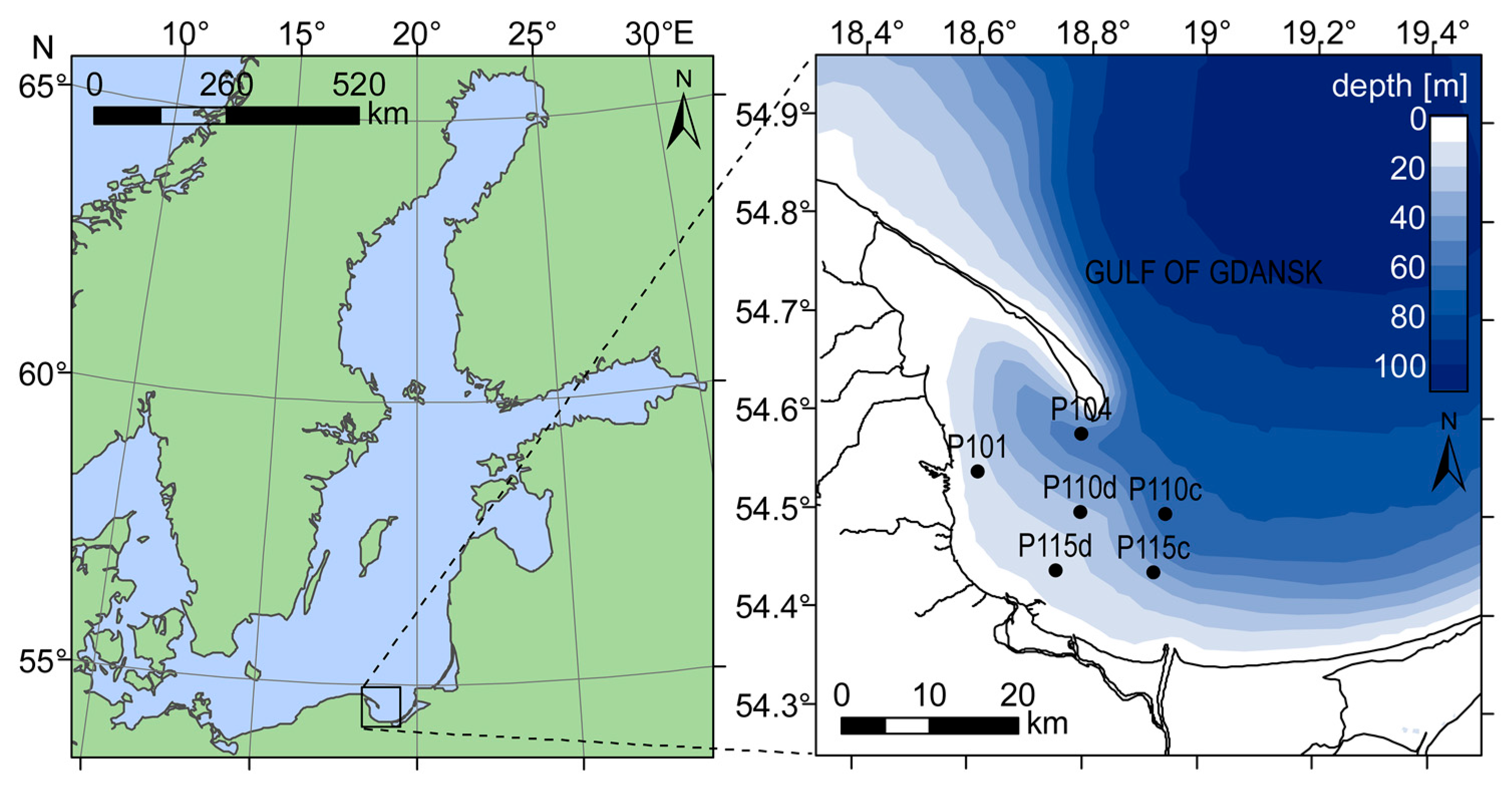
3.1. Field Measurements

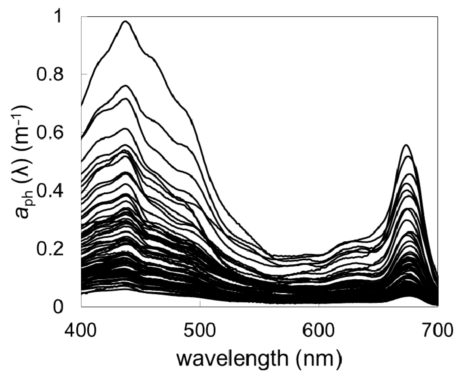
During the study period in the summers of 2012 and 2013, a total of more than 80 data sets were gathered. The phytoplankton absorption spectra varied both in spectral shape and in magnitude (Figure 2).

For example, a_ph (443) varied from 0.036 to 0.954 m⁻¹ (

Table 2. Descriptive statistics for chosen water parameters.

	Min	Median	Max	N
chl˗a	0.69	4.11	31.56	82
PE	0.06	0.56	1.65	82
PC	0.05	2.14	18.94	82
Cell no. of phytoplankton	1.19 × 105	58.03 × 105	19.2 × 106	82
Cell no. of cyanobacteria	100	19.25 × 105	16.6 × 106	82
aph(443)	0.04	0.12	0.95	81
aph(665)	0.02	0.08	0.44	81
adet(400)	0.05	0.14	0.54	81
adet(412)	0.04	0.12	0.48	81
adet(443)	0.03	0.12	0.52	81
aCDOM(400)	0.36	1.12	7.73	63
aCDOM(412)	0.30	0.90	3.90	63
aCDOM(443)	0.20	0.51	2.29	63

). The highest variability, spanning over two orders of magnitude, was noted in the case of chl-a and a_CDOM (443) (Table 2). The highest values of a_ph (λ), as well as chl-a, were observed in June 2013. These parameters showed also the strongest correlation (

Table 3. Correlation matrix depicting the relationships amongst the water parameters (N = 62). The correlation coefficients that were not statistically significant (p < 0.05) are marked in grey.

	chl˗a	aph(443)	aph(665)	adet(443)	aCDOM(443)
chl-a	1.00
aph(443)	0.88	1.00
aph(665)	0.90	0.89	1.00
adet(443)	0.37	0.1	0.58	1.00
aCDOM(443)	0.80	0.80	0.62	−0.084	1.00

). However, the correlation between chl-a and a_ph (665) was slightly stronger (R = 0.90) than with a_ph (443) (R = 0.88). A strong correlation was also observed between a_CDOM (443) and chl-a, a_ph (443), and a_ph (665) (R = 0.80, 0.98, and 0.62, respectively). The weakest, statistically not significant, dependence was observed between a_det (443) and a_ph (443) (R = 0.19) and a_det (443) and a_CDOM (443) (R = −0.08) (Table 3).

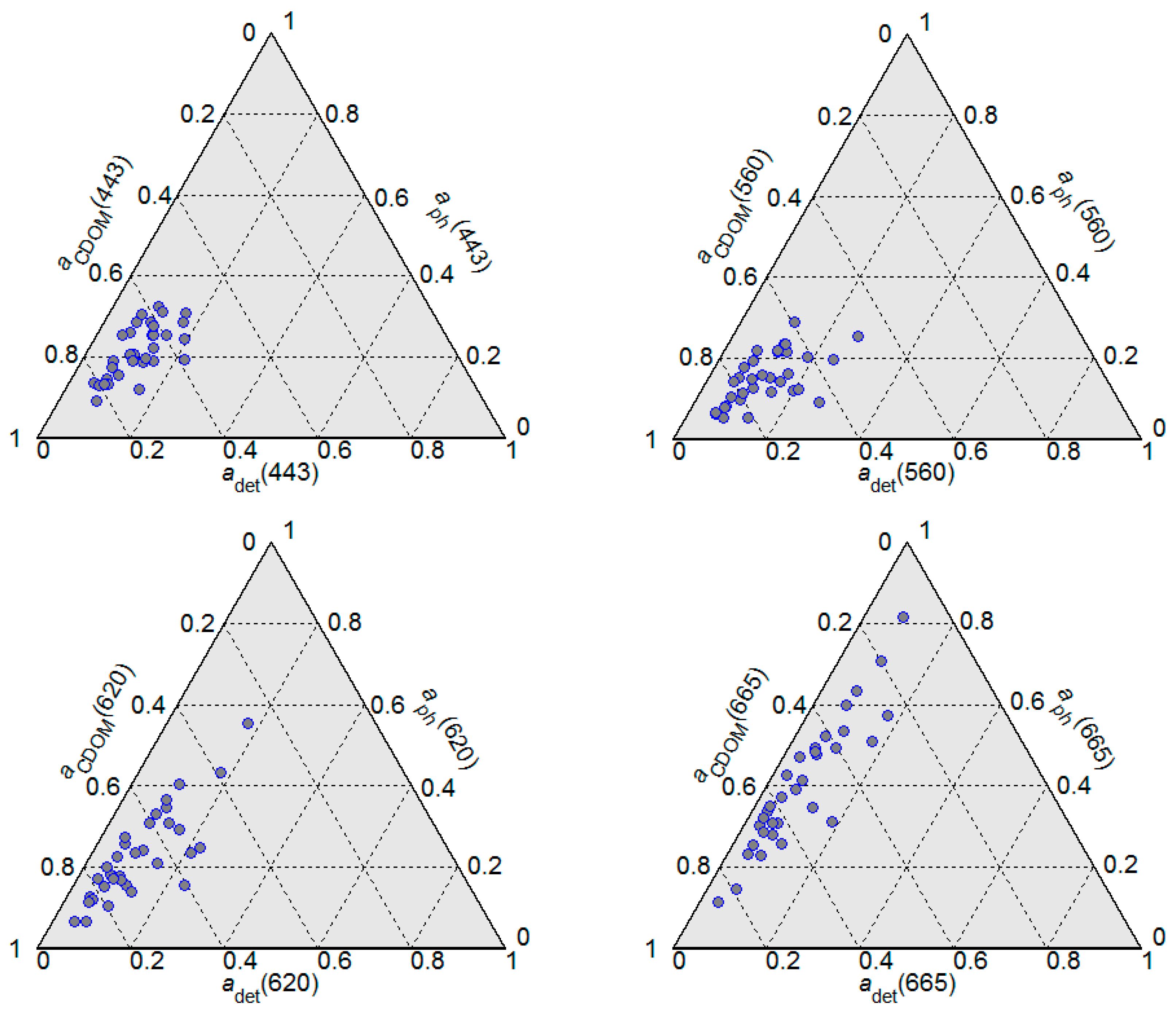
Figure 3 shows the absorption budget for the non-water optically significant seawater constituents, i.e., CDOM, detritus, and phytoplankton pigments at different wavelengths. In all analysed samples, the light absorption at shorter wavelengths (443 nm and 560 nm) was clearly dominated by CDOM which was responsible for roughly 70% of the total absorption. At longer wavelengths, the absorption of light by phytoplankton pigments became more significant. At all analysed wavelengths, the absorption by detritus had the lowest contribution to total absorption.

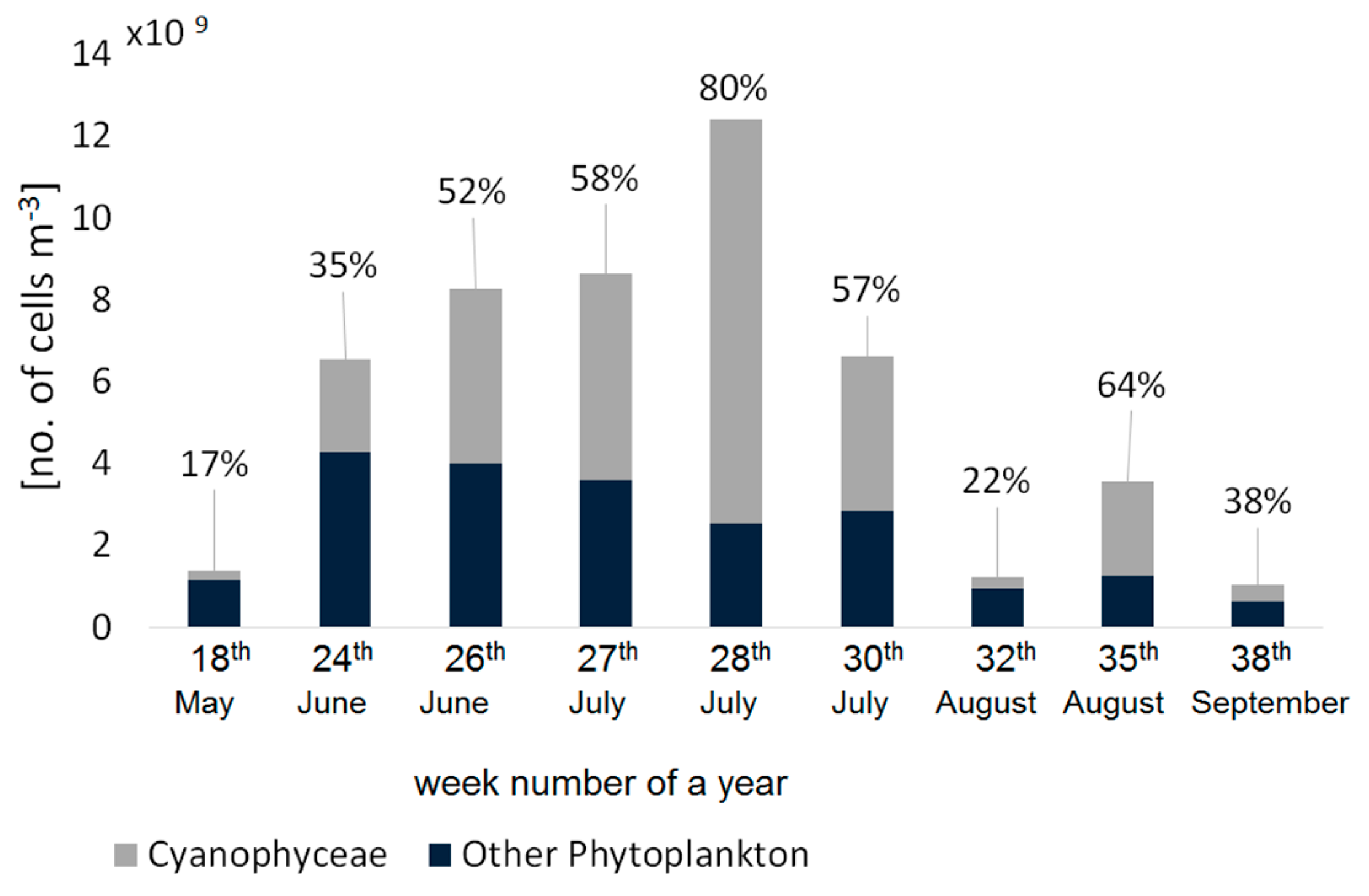
Despite the fact that field measurements were collected only in the Gulf of Gdansk, our dataset covered a wide range of variability of water parameters (Table 2). The cell counts confirmed that during summer, the phytoplankton composition in the Gulf of Gdansk is dominated by cyanobacteria (Figure 4), especially in July, when their contribution to total phytoplankton abundance was >50% in terms of the number of cells per cubic meter.

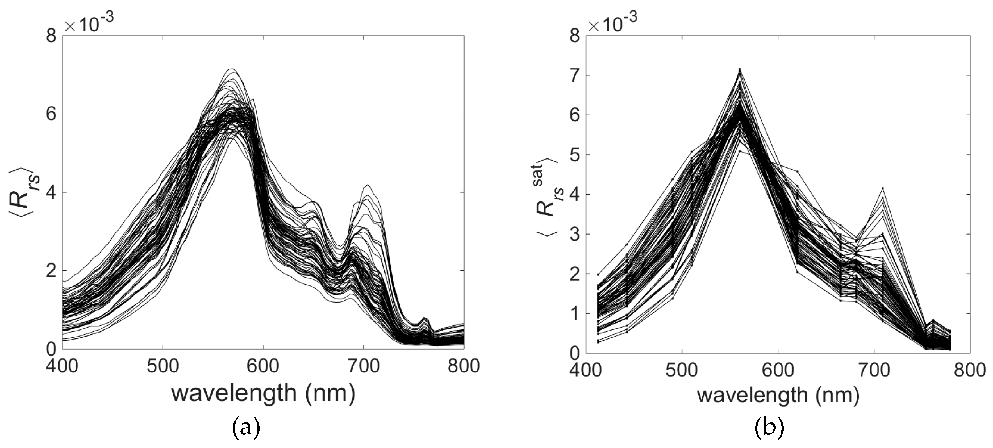
Variability of the optically significant water components influences the shape of the remote sensing reflectance (R_rs) spectra collected in the field campaigns (Figure 5a). The collected R_rs spectra represent quite typical spectral features consistent within optically complex waters [36]. The shape of normalised R_rs spectra shows some interesting features related to the phytoplankton pigment absorption and fluorescence. As expected, the highest reflectance is around 570 nm in the ‘green window’ of minimal chlorophyll absorption and where phycoerythrin absorption is strongest. The trough around 620–630 nm indicates the effect of phycocyanin absorption [59], whereas the trough at about 664 nm indicates the effect of chlorophyll a absorption. Another small peak around 650 nm can be caused by absorption by these two pigments (chlorophyll a and phycocyanin) on either side of the peak. Additionally, phycocyanin fluorescence, which has a maximum at 650 nm, may contribute to this spectral feature [9]. It is difficult to discern the spectral characteristics of phycoerythrin in the R_rs spectral shape. Maximum absorption and fluorescence of phycoerythrin occur around 565 nm and 576 nm, respectively [34], where the other optically significant components (e.g., carotenoids) strongly influence the spectra of R_rs. These features, which are clearly visible in the hyperspectral data (Figure 5a), become less distinct in the R_rs data converted to the multispectral cases (Figure 5b).

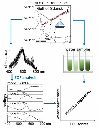
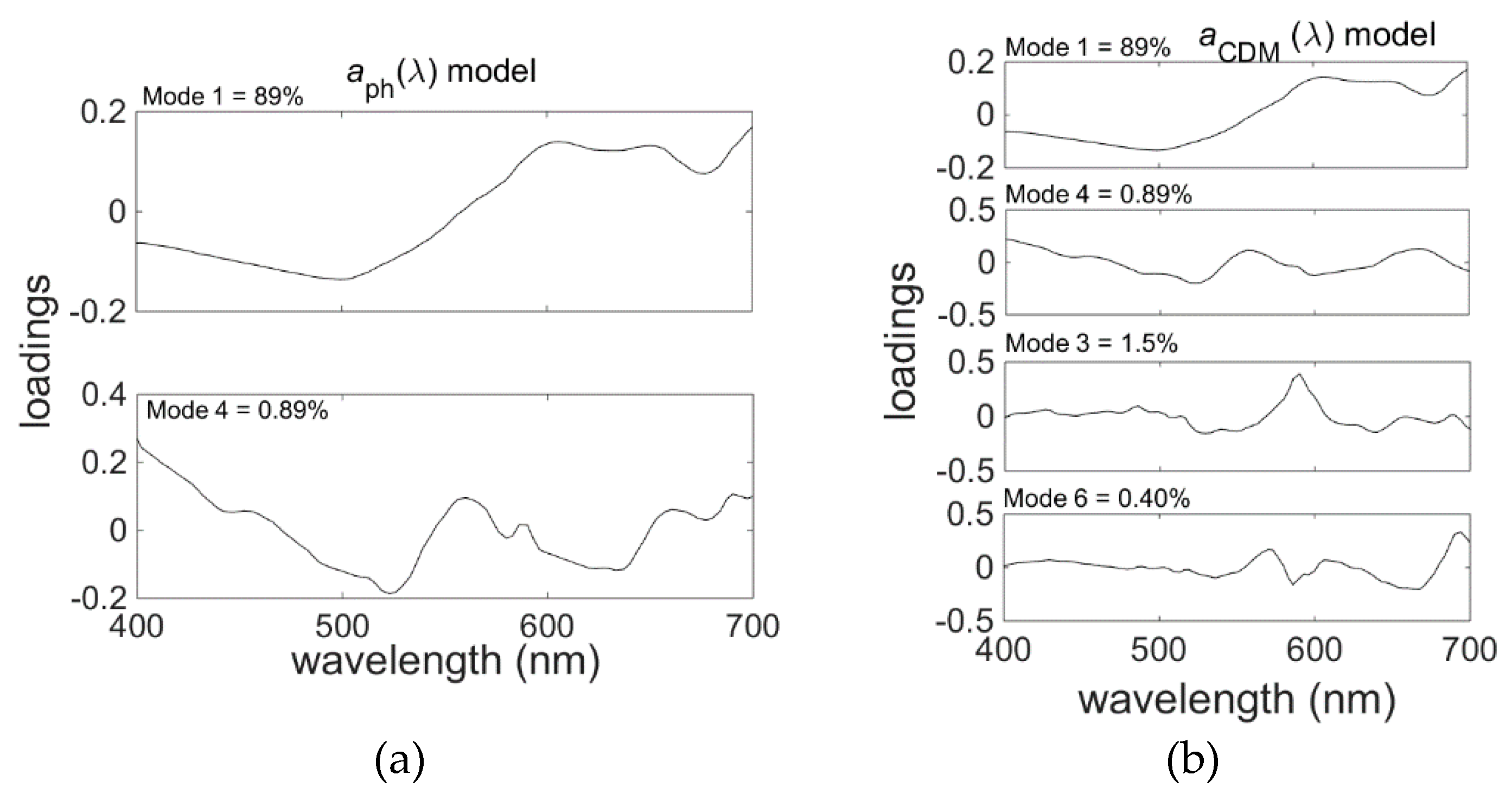
3.2. EOF Models for Phytoplankton Pigments

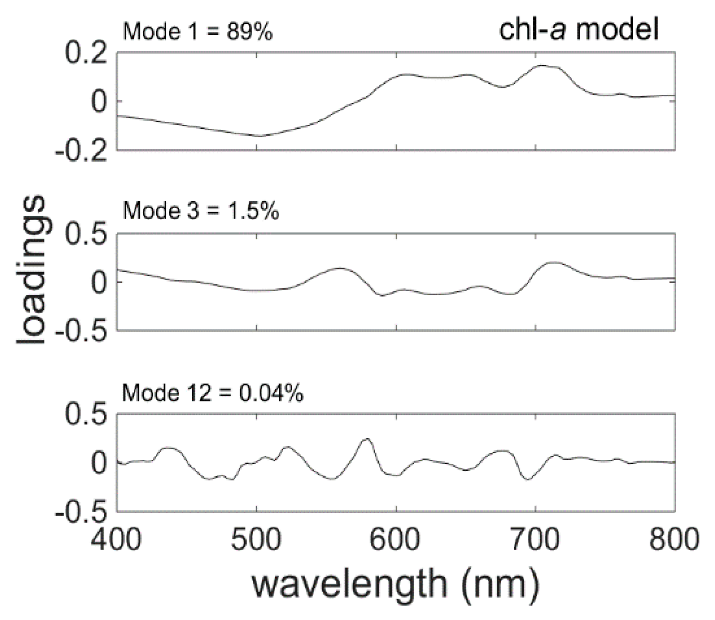
The Chl-a model (4) was based on the three EOFs or modes (

Table 4. Selected empirical orthogonal function (EOF) modes and regression coefficients (4) of the chl-a model.

chl-a model
modes	---	1st EOF	3rd EOF	12th EOF
coefficients	k = 0.71	l1 = 64.6	l2 = 126	l3 = −928

) that were chosen by the stepwise regression. The spectral shapes of these modes, visualised by plotting its loading versus wavelength (Figure 6), may be interpreted as signatures of changes in the optical properties of the water over samples due to changes in the in-water components. The first mode, which captures 89% of the variability in spectral shape, was chosen as the first model component by stepwise fitting. It exhibits a negative correlation between the short and long wavelength regions of the spectrum, implying shifts between the blue-green and red regions of the spectra. That is, the spectral shapes vary such that, whenever the peak around 500 nm is less than average, the band between 600 nm and 800 nm is larger than average, and vice versa. These spectral shifts may be due in part to changes in the concentrations of detritus and CDOM, which are dominating components of the absorption coefficient in the study area (Figure 3). However, variations in the longer wavelengths can only be due to changes in the components of the water column that affect these wavelengths (e.g., phytoplankton pigments).

The second mode chosen by stepwise regression was the 3rd EOF. This mode captures variations in spectral shape centred around 400 nm and 560 nm and in the band from about 714 nm to 800 nm that are positive correlated.

It is worth noting that mode 12, which contains only 0.04% of the variance (Figure 6), was selected by both the SNR procedure and stepwise fit. The numerous spectral inflections, which appear to be coherent signals, are likely related to various phytoplankton absorption and emission (i.e., fluorescence) processes. This strongly implies that mode 12 is not simply noise, as might be expected from such a minor mode of variance, and can bring useful predictive power to the model.

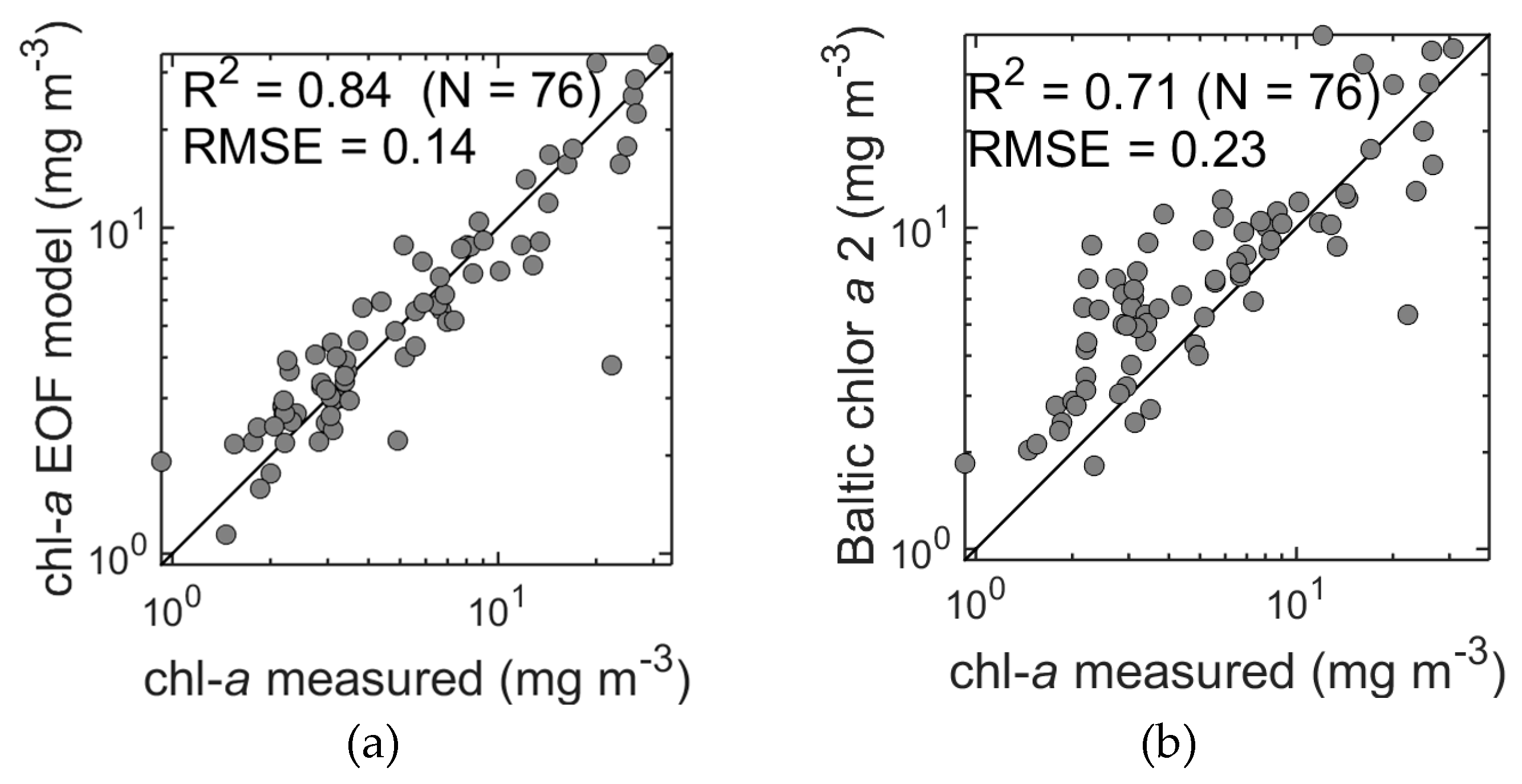
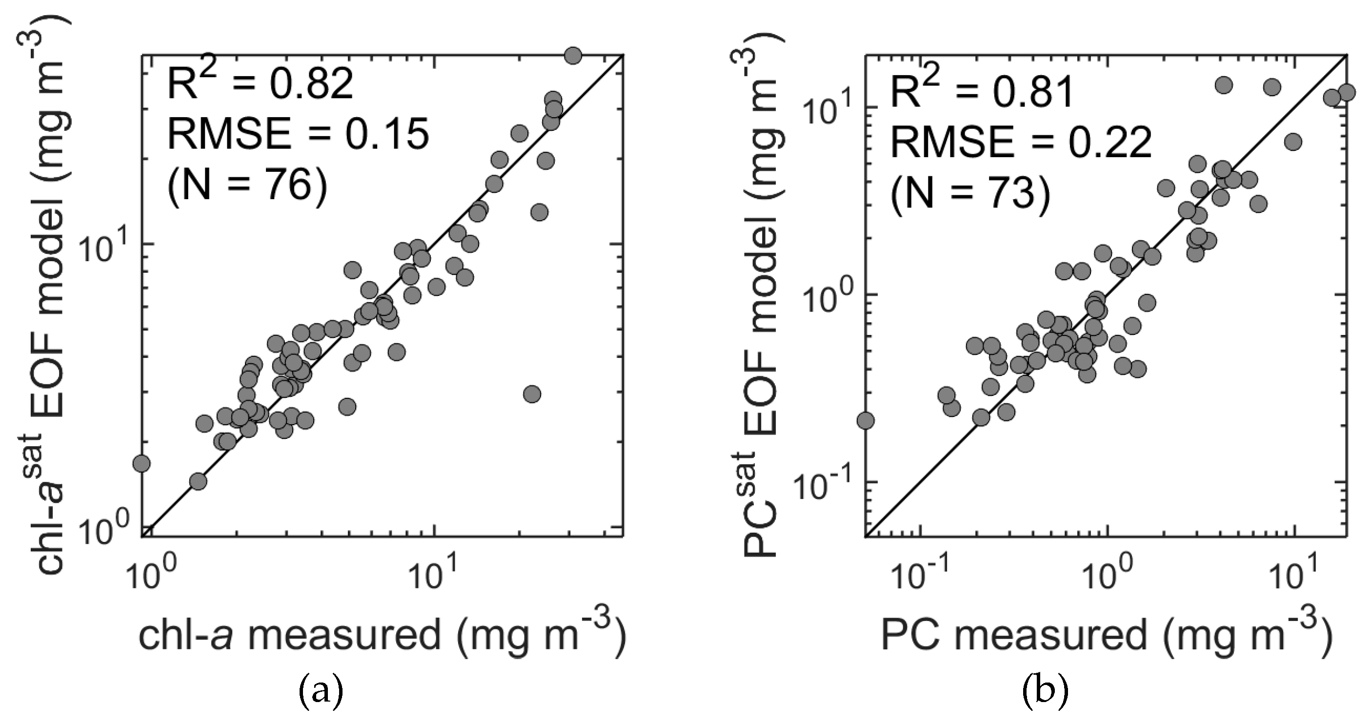
Our model retrieved chl-a from spectral reflectance with an R² value of 0.81 (bias = −0.07 × 10⁻¹⁵), a tight distribution around the 1:1 line (Slope = 0.88, SE = 0.05, Ratio = 1.02) and a relative error (RMSE) of 0.16, even in very optically complex waters (

Table 5. Statistics of the EOF models for pigment concentration. Units are log₁₀(mg·m⁻³) for pigment concentration. Ratio and MPD are dimensionless.

		Pigment Concentration
		PE	PC	chl-a
	N=	70	75	76
R2	All	0.74	0.77	0.84
	X-val	0.64	0.72	0.82
RMSE	All	0.15	0.23	0.14
	X-val	0.18	0.27	0.15
bias	All (×10−15)	0.02	−0.02	−0.09
	X-val (×10−2)	−0.01	−0.03	−0.07
Slope	All	0.84	0.91	0.92
	X-val	0.86	0.88	0.92
SE	All	0.06	0.05	0.04
	X-val	0.06	0.06	0.05
Ratio	All	1.02	0.96	1.02
	X-val	1.03	0.96	1.03
MPD	All	24.57	22.97	16.59
	X-val	26.72	29.73	19.10

, Figure 7a). By contrast, the standard OC4 algorithm applied to our dataset resulted in consistent overestimation of chl-a (R² = 0.73, bias = 0.38, Ratio = 2.43, MPD = 143%, Slope = 0.78, SE = 0.04) and a rather high relative error (RMSE = 0.43). It should be noted here that models such as OC4 are global, whereas our chl-a model was developed using local data. It is therefore not surprising that our model outperformed OC4. However, even with a regionally-tuned band ratio model (Baltic chlor a 2, Table 4 in [22]), chl-a estimates would still be seriously compromised (R² = 0.71, RMSE = 0.23) due to the confounding effect of CDOM absorption at the blue end of the spectrum. The significance of this result is that EOF provides a method to derive accurate chl-a estimates in a scenario where standard approaches provide low quality results.

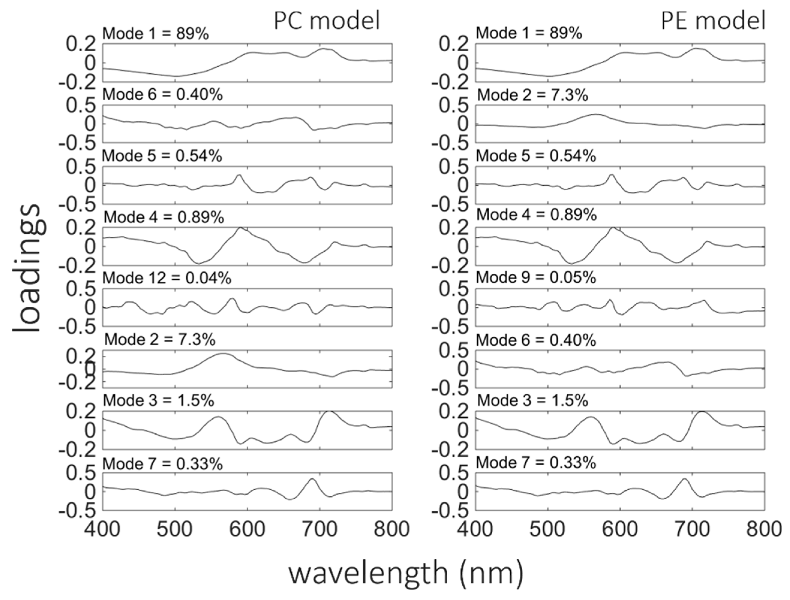
In summer, the Baltic Sea phytoplankton assemblage is dominated by filamentous cyanobacteria species such as A. flos-aquae, N. spumigena, and Dolichospermum sp., and picocyanobacteria species such as Synechococcus sp. [60,61]. The filamentous species, A. flos-aquae, N. spumigena, and Dolichospermum sp., are rich in phycocyanin, while the non-filamentous Synechococcus sp., which significantly contributes to total phytoplankton biomass, is rich in phycoerythrin. Both models, for PC and PE contained eight EOFs modes each (

Table 6. Selected EOF modes and regression coefficients (4) of phycocyanin (PC) and phycoerythrin (PE) models.

PC model
modes	---	1st EOF	6th EOF	5th EOF	4th EOF	12th EOF	2nd EOF	3rd EOF	7th EOF
coefficients	k = 0.15	l1 = 67.4	l2 = −72.2	l3 = 148	l4 = −236	l5 = 318	l6 = 396	l7 = −211	l8 = −1531
PE model
modes	---	1st EOF	2nd EOF	5th EOF	4th EOF	9th EOF	6th EOF	3rd EOF	7th EOF
coefficients	k = −0.34	l1 = 40.6	l2 = −62.0	l3 = −63.1	l4 = −127	l5 = 207	l6 = 131	l7 = −132	l8 = 464

). In both models, the first mode chosen was the first EOF, which captured 89% of the variance in spectral shape. However, the second component was different in both models, as shown in Figure 8 (for PC-left panels and PE-right panels), compared to the chl-a model. In the model for PC estimation, the second component was the 6th mode, which captured only 0.4% of the variance in R_rs spectral shape, while for PE estimation the 2nd mode (7.3% of total variance) was chosen next. For the PC model, the 6th mode has a characteristic peak around 650 nm, where the local maximum in the R_rs spectra due to PC fluorescence is located. In the PE model, the 2nd mode had a peak around 560–570 nm, corresponding to the maximum absorption and fluorescence of PE. These associations help to explain why stepwise regression identified these modes as statistically significant predictors even though they captured only a small proportion of the total variance in R_rs spectral shape.

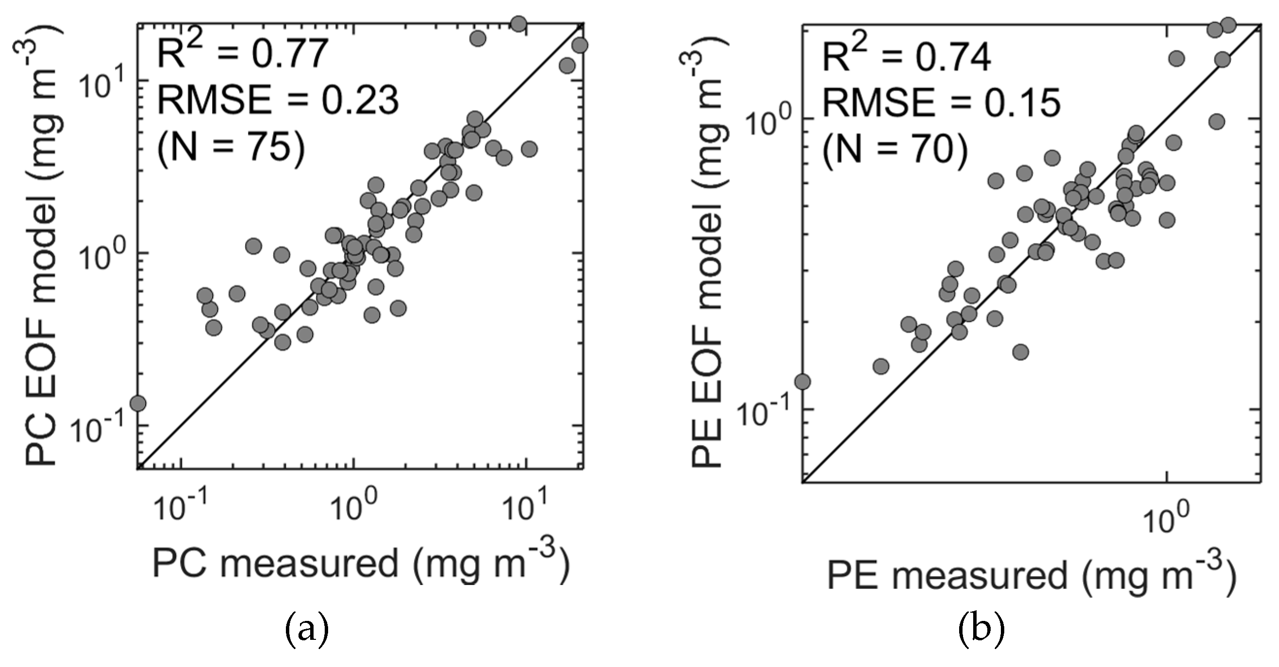
Our EOF models give approximations of PC with R² = 0.73, RMSE = 0.25, MPD = 30% (Figure 9a), and of PE with R² = 0.72, RMSE = 0.15, MPD = 19% (Figure 9b). The EOF model presented here for estimating PC also shows superior results compared to the band ratio model presented by Wozniak et al. [62] for the same study area with MPD = 39%.

Overall, our results (Table 5) compare favourably to a study performed by Bracher et al. [46] who also used the EOF method to retrieve pigment concentrations in Atlantic waters but over a much wider geographical range (roughly 50°N–40°S). They developed models for chl-a, carotenoid pigments, and PE, but not for PC. Their model for chl-a showed a larger relative error with RMSE = 0.49, compared with the RMSE value of 0.16 found in our studies, and a MPD of 43%, compared to our MPD of 19% (Table 5). In the case of PE estimation, our model showed superior results with RMSE = 0.15 and MPD = 19.5%, compared to Bracher et al. [46] who observed RMSE = 1.16 and MPD = 139%. The superior performance of the EOF approach in our study can most likely be explained, in large part, by the fact that the Bracher et al. [46] models were derived over a larger dynamic range, encompassing several biogeographical provinces. In contrast, our study took place exclusively in the Gulf of Gdansk, a body of water that spans over less than 1° of latitude (Figure 1). In several implementations of the EOF approach, authors have noted that the models perform best when trained in a region-specific manner [41,42,47]. However, more recent studies suggest that global implementations may be possible if a dataset with a dynamic range wide enough in parameter space is used to train the models [63].

3.3. EOF Models for Spectral Absorption of Phytoplankton and Coloured Detrital Matter

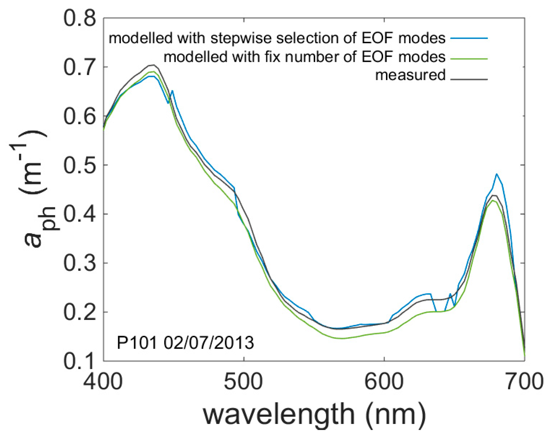
EOF models for phytoplankton and coloured detrital matter (CDM) absorption spectrum were developed separately for each wavelength from the range of 400 nm to 700 nm with a step of 3 nm. Using stepwise regression for each wavelength separately produced spectral discontinuities (Figure 10). This is in part due to differences in the modes chosen for each wavelength. To remove these discontinuities, it was necessary to select a common set of modes for all wavelengths (

Table 7. Selected EOF modes and regression coefficients (4) of the a_ph model.

aph model
modes		coefficients
	λ=	416	442	489	509	513	560	620	663	680
---	k=	−0.73	−0.71	−0.89	−1.03	−1.06	−1.36	−1.33	−1.12	−0.98
1st EOF	l1=	50.7	50.0	49.9	50.4	50.3	50.1	56.1	56.0	55.9
4th EOF	l2=	119.5	143.9	191.3	192.4	195.8	158.7	118.0	85.3	103.3

and

Table 8. Selected EOF modes and regression coefficients (4) of the a_CDM model.

aCDM model
modes	coefficients
	λ=	400	412
---	k=	0.13	0.05
1st EOF	l1=	33.8	33.4
4th EOF	l2=	−84.5	−80.0
3rd EOF	l3=	−54.3	−52.5
6th EOF	l4=	−56.5	−65.5

, Figure 11). The resulting models give accurate predictions for the spectral model products (

Table 9. Statistics of EOF models for phytoplankton and CDM absorption coefficients for chosen wavelengths. Size N = 62 and N = 38 for aph and aCDM, respectively. Units are log₁₀(m⁻¹). Ratio and MPD are dimensionless.

		aph (λ)								aCDM (λ)
	λ=	415	442	490	510	560	620	665	680	400	412
R2	All	0.87	0.86	0.84	0.85	0.82	0.85	0.88	0.89	0.91	0.89
	X-val	0.86	0.85	0.83	0.84	0.80	0.84	0.87	0.88	0.84	0.83
RMSE	All	0.10	0.10	0.11	0.11	0.12	0.12	0.10	0.10	0.06	0.06
	X-val	0.10	0.10	0.12	0.11	0.12	0.12	0.10	0.10	0.07	0.07
bias	All (×10−16)	−0.43	−0.47	−0.18	−0.97	−1.52	−4.51	2.77	−1.15	0.30	0.04
	X-val (×10−3)	−0.08	−0.18	−1.19	−0.63	−0.39	−1.33	−0.88	−1.03	−1.05	0.21
Slope	All	0.91	0.90	0.86	0.86	0.86	0.91	0.93	0.93	0.95	0.95
	X-val	0.93	0.93	0.92	0.92	0.90	0.92	0.94	0.94	0.95	0.95
SE	All	0.04	0.05	0.05	0.05	0.05	0.05	0.04	0.04	0.05	0.05
	X-val	0.05	0.05	0.05	0.05	0.06	0.05	0.05	0.05	0.06	0.06
Ratio	All	0.99	0.98	0.98	0.99	0.96	0.97	0.99	0.98	1.03	1.02
	X-val	0.99	0.99	0.99	0.98	0.97	0.98	1.00	0.99	1.02	1.02
MPD	All	12.09	10.23	12.22	12.11	17.34	16.47	10.33	11.17	7.72	8.47
	X-val	12.42	11.22	13.12	13.26	18.04	18.34	12.95	12.51	10.64	10.55

). Nevertheless, the discontinuities are the subject of ongoing investigation and future work will seek to develop more objective methods to eliminate this problem.

Knowledge of the shape of the phytoplankton absorption spectra is needed in models that estimate phytoplankton chlorophyll concentrations [64,65], or as an input into bio-optical models that predict carbon fixation rates for the global ocean [66,67,68]. The shape and the magnitude of the phytoplankton absorption spectra is controlled primarily by the concentration of various photosynthetic and photoprotective pigments and by the level of the pigment package effect within the cells. The influence of these two processes varies with depth, phytoplankton species composition, and cell size. Quantification of CDM plays an important role in understanding the oceanic carbon cycle. Moreover, CDM absorbs strongly in the UV and blue range of the spectrum, thus determining phytoplankton and bacterial productivity [69]. 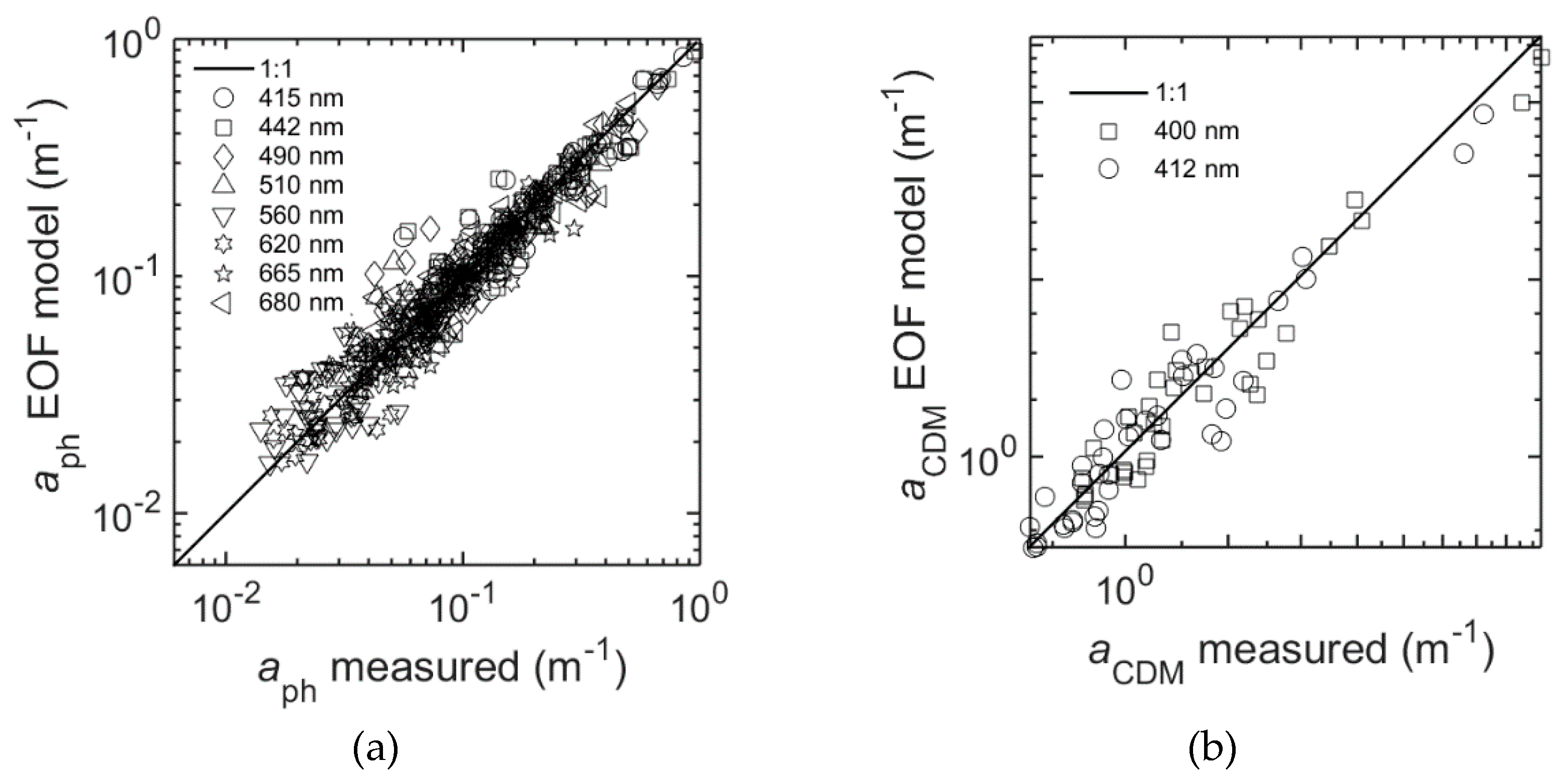Figure 12a and Table 9 present the results of the EOF model for a_ph at selected wavelengths: R² (λ) ranging from 0.80–0.89, and RMSE (λ) = 0.10–0.12.

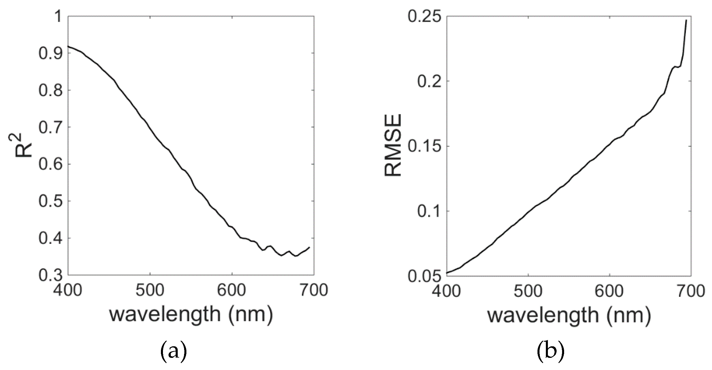
The EOF model for a_CDM gave the best results for the wavelengths in the blue spectral range between 400 and 450 nm; R² was higher than 0.6 and RMSE was around 0.06. The model skill decreased with increasing wavelengths (Figure 13), reaching R² below 0.40 and RMSE of about 0.25 for λ = 700 nm. The contribution of CDM to the total absorption decreases approximately exponentially with increasing wavelength, which would explain the model’s decreasing skill towards the red region of the spectrum. However, a_CDM absorption spectra can be derived from the following formula [1]:

$$a_{CDM}(\lambda )=a_{CDM}({\lambda }_0)\cdot e^{-S(\lambda -{\lambda }_0)}$$

(9)

where the slope value S can be retrieved when a_CDM is given for at least two wavelengths, for example 400 and 412 nm (Figure 12b) which can be estimated with good agreements (Table 9) by the EOF model.

An inverse semi-analytical model for a_ph and a_CDM was presented by Wei and Lee [1] and Werdell et al. [70], but in both cases our model showed better results. The model of a_CDM presented by Wei and Lee (2015) also showed similar errors as our model, where model performance was proven to become worse with increasing wavelengths (Figure 13).

3.4. EOF Models for Synthetic Satellite Data

The EOF method applied to the synthetic satellite data set (Figure 5b) showed accurate results despite the reduced spectral resolution. The accuracy of chl-a estimates was found to be slightly reduced compared to estimates from hyperspectral data (R² = 0.82, RMSE = 0.15 and MPD = 18%, R² = 0.84, RMSE = 0.14, and MPD = 17%; Figure 7a and Figure 14a, respectively). Unexpectedly, PC estimates (Figure 14b) were actually more accurate compared to the values obtained from the hyperspectral data in terms of R², RMSE, and bias (R² = 0.81, RMSE = 0.22, and MPD = 33%, R² = 0.77, RMSE = 0.23 and MPD = 23%; Figure 9a and Figure 14b, respectively). A possible reason for this may lie in the, as yet, imperfect approach to thresholding noise in the hyperspectral data, i.e., unfiltered hyperspectral noise may degrade the PC estimates. Cross validation was again performed and confirmed the robustness of the models. This demonstrates that a reduction of spectral information from hyper- to the multispectral potentially has little impact on predictive accuracy, and in the case of the PC estimates, actually improved the results. Similar results were found by Craig et al. [41] for MERIS data, who suggested that as long as spectral information pertinent to the parameter of interest was included in the multispectral waveband set, the EOF models would perform similarly to their hyperspectral versions. In this case, wavebands that included the spectral characteristics of the absorption of chlorophyll a were included in the synthetic data, hence retaining the information required for their accurate prediction.

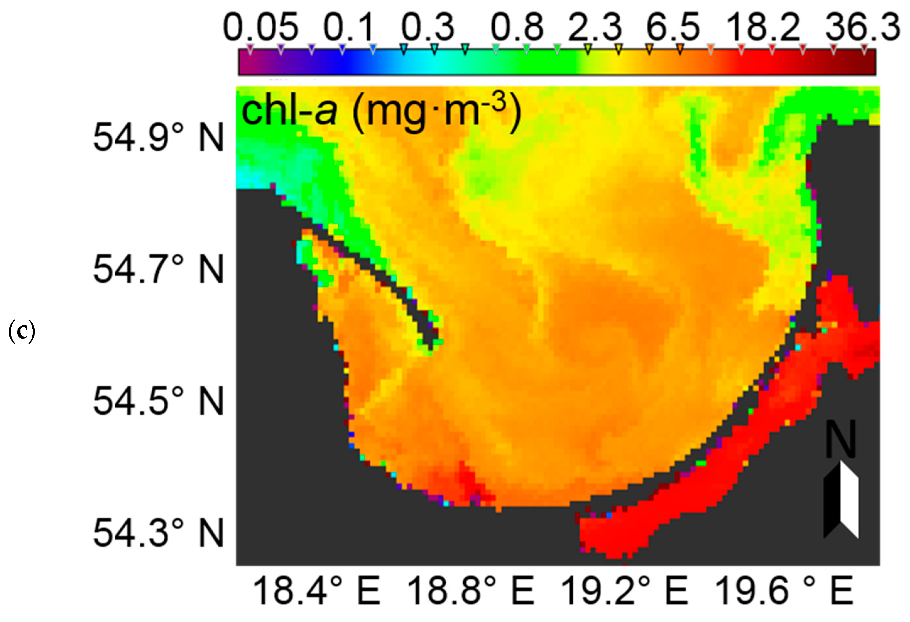
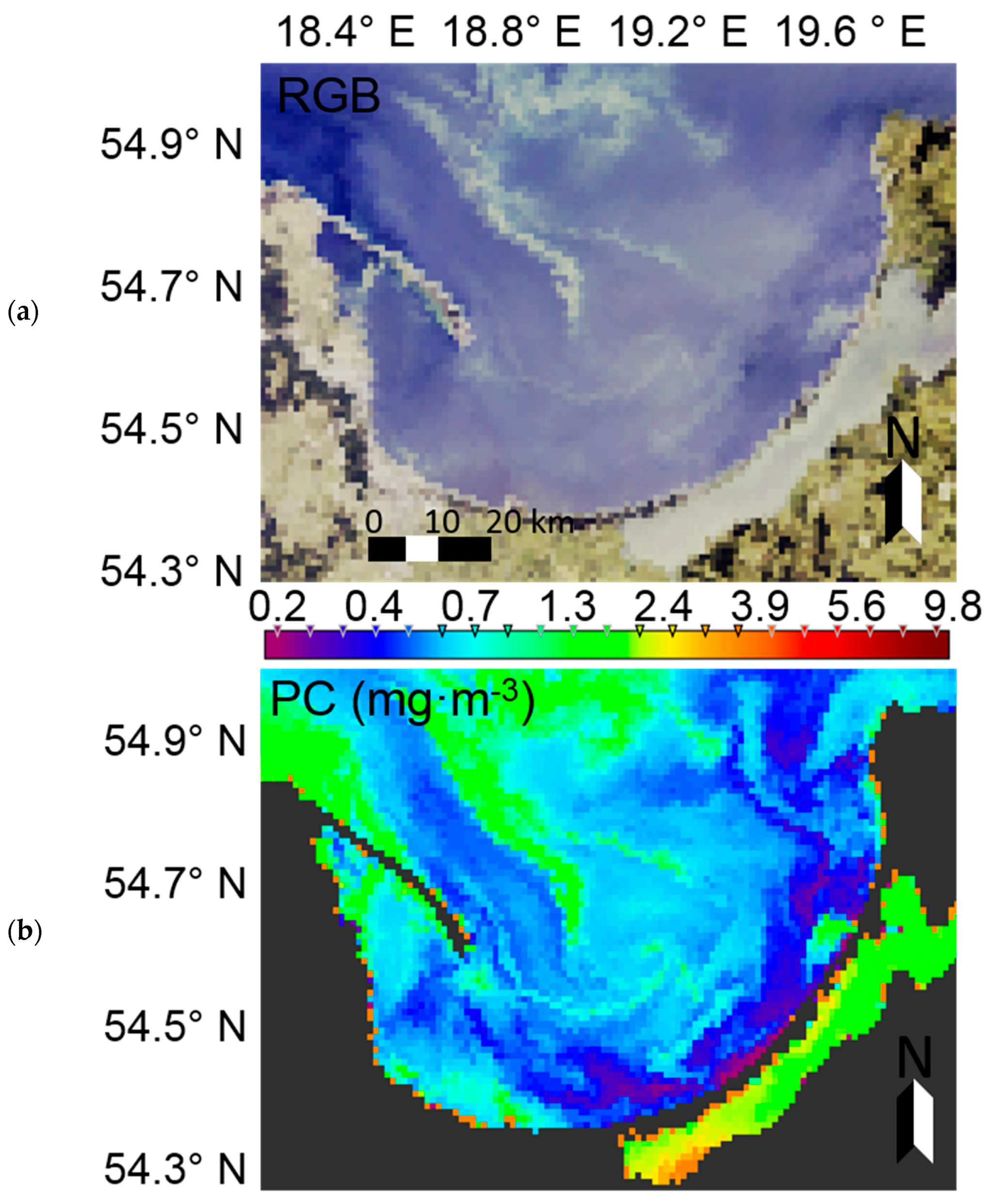
At the time of preparation of the manuscript, summer data from the European Space Agency’s Sentinel-3 instrument, OLCI (Ocean and Land Colour Instrument) radiometer were not yet available. Therefore, to demonstrate the potential usage of EOF models to characterise phytoplankton blooms in the Baltic Sea, MERIS (Envisat) data were used. The Case-2 Regional (C2R) processor [71] was used to derive remote sensing reflectance from MERIS level 1b data acquired on 5th July 2010 in the Gulf of Gdansk. The EOF models were then run to calculate PC (marker pigment of cyanobacteria in the Baltic Sea) and chl-a (proxy of phytoplankton biomass). In the surface water of the RGB image, an algal bloom is clearly visible in the northern part of the image (Figure 15a). Considering the time of data acquisition, it likely represents a cyanobacteria bloom. Evaluating the PC dynamics (Figure 15b), a similar pattern is evident, further supporting the likelihood that the RGB feature is, indeed, a phytoplankton bloom and most likely dominated by cyanobacteria. In the southern area of the Gulf of Gdansk, where the Vistula River strongly influences the water properties, chl-a is much higher when compared to the PC concentration. This may be explained by the fact that the input of freshwater increases nutrient concentrations, and thus allows other phytoplankton groups which do not contain PC to outcompete cyanobacteria. These are preliminary results, which may need further investigation and validation, but they demonstrate the potential usefulness of the EOF models for satellite data.

4. Conclusions

We present EOF models based on R_rs spectra collected in the optically-complex waters of the Gulf of Gdansk, which are strongly influenced by CDOM absorption to predict the pigment concentration and absorption spectra of phytoplankton and coloured detrital matter (with R² > 0.79 for all models). The models presented here show much improved retrieval when compared to OC4 or even local band ratio models. For areas that possess similar ranges of optical constituents and ranges of pigment concentration (up to 20 mg·m⁻³ for PC and 35 mg·m⁻³ for chl-a), the model should work well. However, for areas outside the tested range, a new EOF model may have to be developed. The results of the EOF models applied to data with reduced spectral resolution also show good agreement with the in situ measurements, yielding a prospect of using this method in near real-time satellite systems. The estimation of the concentration of pigments from the phycobilin group can be used for monitoring and detection of filamentous, and potentially toxic, cyanobacterial blooms.

In the future, EOF models need to be validated against satellite data. However, the results now available already indicate the applicability of the EOF method to multispectral satellite data such as OLCI (Sentinel-3), assuming that accurate atmospheric correction can be achieved.