
Mapping the Expansion of Boom Crops in Mainland Southeast Asia Using Dense Time Stacks of Landsat Data
by
 , and
, and
Kaspar Hurni
1,* ,
,
Annemarie Schneider
2,3,
Andreas Heinimann
4,5,
Duong H. Nong
6 and
Jefferson Fox
1 1
East-West Center, 1601 East-West Road, Honolulu, HI 96848, USA
2
Center for Sustainability and the Global Environment, Nelson Institute for Environmental Studies, University of Wisconsin–Madison, 1710 University Avenue, Madison, WI 53726, USA
3
Department of Geography, University of Wisconsin–Madison, 550 North Park Street, Madison, WI 53706, USA
4
Centre for Development and Environment, University of Bern, Hallerstr. 10, CH-3012 Bern, Switzerland
5
Institute of Geography, University of Bern, Hallerstr. 12, CH-3012 Bern, Switzerland
6
Faculty of Environment, Vietnam National University of Agriculture, Trau Quy, Gia Lam, Hanoi 131004, Vietnam
*
Author to whom correspondence should be addressed.
Remote Sens. 2017, 9(4), 320; https://doi.org/10.3390/rs9040320
Submission received: 23 December 2016
/
Revised: 10 March 2017
/
Accepted: 24 March 2017
/
Published: 29 March 2017
(This article belongs to the Special Issue Mapping, Monitoring and Impact Assessment of Land Cover/Land Use Changes in South and South East Asia)
Abstract
:We performed a multi-date composite change detection technique using a dense-time stack of Landsat data to map land-use and land-cover change (LCLUC) in Mainland Southeast Asia (MSEA) with a focus on the expansion of boom crops, primarily tree crops. The supervised classification was performed using Support Vector Machines (SVM), which are supervised non-parametric statistical learning techniques. To select the most suitable SMV classifier and the related parameter settings, we used the training data and performed a two-dimensional grid search with a three-fold internal cross-validation. We worked in seven Landsat footprints and found the linear kernel to be the most suitable for all footprints, but the most suitable regularization parameter C varied across the footprints. We distinguished a total of 41 LCLUCs (13 to 31 classes per footprint) in very dynamic and heterogeneous landscapes. The approach proved useful for distinguishing subtle changes over time and to map a variety of land covers, tree crops, and transformations as long as sufficient training points could be collected for each class. While to date, this approach has only been applied to mapping urban extent and expansion, this study shows that it is also useful for mapping change in rural settings, especially when images from phenologically relevant acquisition dates are included.

1. Introduction
Over the past half century, the five countries of Mainland Southeast Asia (MSEA)—Cambodia, Laos, Myanmar, Thailand, and Vietnam—have witnessed major shifts from predominantly subsistence agrarian economies to increasingly commercialized agriculture and, in the case of Thailand and Vietnam, to industrialized societies. Major drivers of change include policy initiatives that fostered regional economic integration and promoted large-scale infrastructure development, including extensive road-building, rapid expansion of boom crop plantations (e.g., rubber, coffee, etc.), and large-scale hydropower dam construction [1,2,3]. These policy initiatives have led to shifts in smallholder livelihood strategies and natural resource use practices over the past two decades, including agricultural intensification and the linking of smallholder production systems to land, labor, and commodity markets. In a recent survey of agrarian change, Hall et al. [4] identified the three major land-cover transitions in Southeast Asia as being: urbanization, forest loss and gain, and agricultural intensification, including the massive expansion of boom crops.
Boom crops are crops that witness rapid and extensive expansion usually triggered by increased market incentives and favorable policies, e.g., promoting agricultural transformation in the form of smallholder market integration and large scale plantations [5]. As a result the rate of expansion and the type of boom crop varies over time and geographical context. In MSEA the boom crops being promoted and grown on formerly forested areas mainly include tree-based products such as rubber, coffee, fast-growing tree species for pulp and paper (particularly eucalyptus and acacia), cashews, and fruits such as oranges, lychees, longans, etc. Between 2000 and 2010, the extent of the landscape occupied by tree crops grew from 54,860 km2 to 83,710 km2, representing an annual rate of change of 4.3% per year [6]. Boom crops in MSEA are usually developed on land considered by national leaders and others to be ‘resource frontiers’, with low population densities, officially available land, and underutilized resources [7]. In reality, these places are almost always occupied by small-scale farmers, especially upland minorities who have lived there for generations [8,9]. The expansion of boom crops, the investment of political and financial capital they represent, and the concomitant shifts in livelihood strategies and land-use patterns that accompany them represent some of the most profound social and environmental changes in the region in the last century [10,11]. Despite the importance of these transitions, up-to-date maps that depict the precise location, extent, and timing of recent changes do not exist. This is due partially to the difficulty of mapping in a region where persistent cloud cover exists throughout the monsoon period and the fact that a large proportion of farm fields are smaller than 0.5 ha, resulting in a highly heterogeneous and dynamic landscape that requires a monitoring approach using data at Landsat scale or higher spatial resolution. In addition, this topic may have received less priority than other research topics.
Early attempts to map rubber or to estimate rubber stand age relied on single date imagery, but these studies reported poor accuracy because rubber can be confused with secondary growth forest, arable land when it is young, and grassland when it sheds its leaves in the dry season [6,12,13,14]. New approaches using time series imagery have been effective for resolving these issues, because multiple images over the course of one year can capture rubber’s distinct defoliation period in January and February [15]. Methods to effectively handle large quantities of temporal and spectral data have included principal component analyses of image pairs [16], phenology-based image differencing and thresholding [17], and the use of trend algorithms to map forest disturbance related to rubber plantations [18]. These Landsat-based approaches remain limited by frequent cloud cover, however, which has led to the emergence of data fusion methods combining radar and multispectral imagery [19,20,21,22,23]. These approaches work well for mature rubber, but face difficulties classifying young rubber and differentiating rubber from deciduous forest. Still other approaches deal with cloud issues by applying methods that take advantage of the daily revisit time and 16-day image composites from MODIS 250 m data [24,25]. The relatively large pixel size from MODIS, however, is not suitable for mapping the highly heterogeneous landscape in MSEA at local scales [26,27]. We build on both the MODIS- and Landsat-based approaches to develop a method that effectively captures not only rubber, but changes in other tree crops (e.g., cashews, coffee, and eucalyptus), other land conversions (e.g., sugarcane), rotational agriculture, and hydropower dam expansion.
In this study, we applied a supervised classification of Landsat dense time stacks using support vector machines (SVMs) to map changes in forest-dominated landscapes at local (<1 ha) and regional scales, with a specific focus on the expansion of new tree crops from 2000 to 2014, deforestation, and secondary tree cover associated with rotational agriculture. Considering the variety of land cover types, land cover phenology, and land cover transitions, this research had two objectives: (1) to map boom crop expansion by classifying the time of change (within 3 year time frames) and the ‘from what—to what’ process of change and to map other dominant land cover and change types; and (2) to provide a thorough assessment on how seasonal image selection, classification scheme, and the sample points affect the parameterization of the SVM classifier and the accuracy of the classification. We mapped eight persistent land cover types (including multiple forest and agricultural classes), the ongoing transitions to boom crops (rubber, cashews, eucalyptus, sugarcane, and coffee), as well as additional agricultural changes (rotational agriculture, conversion of forests to annual agriculture or built-up land). To capture the heterogeneity of the MSEA landscape, we chose seven Landsat footprints with different land-cover configurations and dynamics. For each footprint we then selected multi-seasonal images with acquisition dates that represent the characteristic phenology of the main land-cover and land-use (LCLU) types. Using a combination of local knowledge, field-collected information, very high resolution Google Earth time series imagery, and Landsat data, we selected classification training and verification points for each footprint for input to the SVM classifier. Using the training points, we assessed the optimal parameter configuration of the SVM algorithm and trained the classifier. We then performed the accuracy assessment using the verification points to obtain information on the performance of the approach for classifying land cover dynamics in the region. Classification results as well as training and verification points for each footprint are available online [28].
2. Materials and Methods
2.1. Study Area
We selected three Landsat footprints in the northern highlands (Myanmar, Thailand, Laos), and four footprints in the southern lowlands of the MSEA region (Laos, Cambodia, Vietnam; see Figure 1). The selection of study areas was based on three criteria. First, these areas corresponded to locations in northeastern Cambodia and southern Laos where within this project household interviews were being conducted. Experiences from these field visits and field photos provided information on the transformation processes and supported the collection of classification samples. Second, we have geospatial data on agricultural land concessions in Laos and Cambodia that provide initial insights as to where LCLUC may occur, but that also provide information for assessing the validity of the maps produced in this study. Finally, we selected the seven footprints because of variability in the rates, patterns, and types of change that occur across the region. The heterogeneity of the landscape, the piecemeal nature of land conversion and land-cover change, and the frequency of cloud cover make these areas some of the most challenging for monitoring change with satellite data. Therefore, the seven footprints serve as case studies for developing a generalizable approach for routine monitoring of boom-crop expansion, forest loss, and rotational agriculture.
In addition to differences in climate and physical geography, the unique political and economic histories of these countries have produced different LCLUC trajectories (Table 1). In Thailand (13047, 126049, 126050), vast areas are covered by permanent annual agriculture; fruit and rubber are the prevailing tree crops, mostly planted by smallholders [1,29]. Most of the expansion of rubber and fruit trees occurred in the middle of the 20th century, and, due to favorable policies and world market prices, another boom in rubber occurred after 2003 [30,31]. In Vietnam (125049), the expansion of tree crops started after the Doi Moi economic reforms of 1986. Conversions to coffee began in the 1990s while rubber expanded steadily from an area of 81,100 ha in 1990 to 548,000 ha in 2013 [29,32]. Land reforms were initiated during the 1990s in Laos, but boom crops mainly emerged in the last 10 to 15 years [3,33]. In Northern Laos (12046) smallholder rubber plantations dominate, while in the South (126049, 126050, 125050) smallholder and large scale plantations of rubber, eucalyptus, sugarcane, and coffee (introduced in the 1960s) occur [3,34]. Rotational agriculture is still widespread in Laos, especially in the northern uplands [2].
Cambodia (125050, 125051) witnessed an increase in large scale rubber plantations in recent years linked to the 2001 land law that allows the Royal Government of Cambodia to allocate land concessions for commercial purposes [35,36]. A substantial portion of footprint 125051 has been approved for boom crop plantations (Figure 1). Rotational agriculture is less common in Cambodia than Laos, and smallholder plantations of cashews and rubber have been established [1]. Expansions of rubber concessions have occurred in Myanmar (131046) over the last 10 to 15 years as a result of ceasefire treaties in the Myanmar-China borderlands and on-going political transitions [37,38].
2.2. Data Sets and Initial Processing
This study relied on four unique datasets: (1) Landsat images spanning 2000 to 2014; (2) field interviews and photographs; (3) Google Earth imagery; and (4) agricultural land concession data. To capture the distinct phenology of different land-cover types and land-use activities, we selected Landsat images with acquisition dates from multiple seasons during the fifteen-year study period (Figure 2). Distinguishing rubber from forests, for example, requires capturing the timing of rubber’s leaf defoliation (January, February) and the rapid re-greening phase (March, April) [15]. Deciduous forests, on the other hand, stay defoliated throughout the dry season and do not foliate as fast or as intensively as rubber [39]. As a result, deciduous forests show a decline in greenness over the course of the dry season and can be differentiated from other land-cover types using imagery collected from December to April.
Other tree crops (e.g., cashews, eucalyptus) do not shed their leaves and therefore do not show a phenological pattern as distinct as rubber [40]. For these land-cover types, the number of high quality observations is therefore more important than the selection of appropriate image acquisition dates. Where possible, images from the growing season are included to distinguish tree crops other than rubber; however, cloud-free data from May to September are almost non-existent in monsoon Asia [41]. Finally, arable land and grassland are both represented by the low vegetation areas class (including mainly permanent annual agriculture, but also built up areas, grasslands, bare areas, rock formations, etc.); these areas can be distinguished from the substantial green cover of the forest and tree crop classes (identifiable across multiple images per year) because of their sparse vegetation cover or lack of cover throughout the year.
Based on these requirements we selected Landsat 5, 7, and 8 images from the surface reflectance products available at EarthExplorer [42]. We excluded images with cloud cover >20%, selected images from the target seasons (November–December, January–February, March–April, Figure 2), and included a wet-season image (May–October) whenever good observations were available (Figure 3). If the seasonal imagery contained partial cloud cover, we compensated for this gap in the time series by collecting additional images with close acquisition dates. Similarly, when only Landsat 7 data with the failed Scan Line Corrector (SLC-off data) were available, we used a greater number of observations for each season. In total, 2–9 images per year were selected for each of the seven footprints, resulting in a total of 60–74 Landsat scenes per footprint. We then checked the amount of valid data for each pixel (i.e., count of non-clouded and non-SLC-off pixels). Clouds and haze distribute rather randomly and we found their effects on the spatial distribution of valid pixels to be limited. This was different for the Landsat 7 SLC-off images, which represent the majority of the data we used (see Figure 3). Due to the SLC-off gaps, the amount of valid data is reduced towards the eastern and western edges of all footprints. These edge pixels tend to show approximately one third of the amount of valid pixels compared to the centers of the scenes. This could affect the quality of the classification, but we expect this effect to be limited because more than 90%–95% of all pixels of each footprint show an average of more than three valid observations for each year [43,44].
We checked the geometric accuracy of the time series and found the standard terrain correction applied to Level 1T data to be sufficient [45]. While radiometric normalization is not required when analyzing images simultaneously rather than individually, we opted for the surface reflectance product as it increases the spatial and temporal consistency of the time series [42,46,47,48].
Given the dense time stacks of data, there was no need to mask SLC-off gaps and clouds. With a large number of good observations, clouds and SLC-off gaps can be treated as noise with a negligible effect on classification accuracy [43]. However, to reduce the heterogeneity of areas without data and to obtain a more consistent time series, we assigned clouds and cloud shadows the same value as the SLC-off gaps. To improve the performance of the classifier, we also performed a linear stretch of the image bands by cutting off the top and bottom one percent and assigning a value range from 0 to 1 [49,50,51]. We then stacked all multispectral layers to create a multi-date composite for each footprint, and used these as input to the SVM classification algorithm.
This study relied heavily on additional data sources. We collected field photos of all land-cover types in northeastern Cambodia and southern Laos on three separate field visits (two carried out in July 2014 and one in November 2015). The photographs overlapped with only a few of the seven Landsat scenes and do not provide any historic information, but they allowed us to link canopy patterns of tree crop plantations as observed in Google Earth with specific tree crops (e.g., the row structure of rubber and cashew plantations, see Figure 2). Such information was crucial for collecting classification training and verification samples across the seven Landsat footprints. To supplement the on-site observations, we also used the time series of high resolution imagery in Google Earth, as well as the inventories of boom crop land concessions that were available for Laos and Cambodia [3,36].
2.3. Classification Scheme and Training and Verification Data
We developed the classification scheme in an iterative process that considered all four datasets described above. Based on local expert knowledge and information from the field visits, we defined the classification scheme to include the targeted change classes (boom crop expansion) and the prevailing stable land cover types (Table 2). During the collection of training and verification points, we then added classes when they occurred frequently within the study area (e.g., pineapple plantations in Thailand, footprint 130047). The final classification scheme is comprised of: (1) land-cover types that do not change between 2000 and 2014 (no change), including water, evergreen forests, deciduous forests, low vegetation areas, and stable crop classes (rubber, cashews, pineapple, and fruit trees planted before 2000); (2) boom crop expansion classes, including rubber, cashews, coffee, eucalyptus, and sugarcane; and (3) an additional set of land cover change classes that were not the primary focus of this work (other change, e.g., rotational agriculture, changes in low vegetation areas, etc.). Note that for Group 2, we mapped the type of change (i.e., from evergreen forests, deciduous forests, or low vegetation areas to boom crops) as well as the time of change in three-year time steps for five periods (2000–2002, 2003–2005, 2006–2008, 2009–2011, 2012–2014). Given the limited availability of historic high resolution imagery, it was not possible to define the time of change reliably on a yearly basis. For the Group 3 classes, we only considered the type of change (e.g., existence of a crop-fallow rotation cycle), but did not specify the period of change. The Group 3 classes include rotational agriculture (defined here as any form of land use with two or more years of fallow), conversion to low vegetation areas (mainly expansion of permanent annual agriculture, including the intensification from crop-fallow rotation land use to permanent agriculture), and expansion of water related to new hydropower dam construction.
To collect training and verification points, we generated 1000 random points for each footprint and assigned the land cover or change class as follows:
- We linked the field photos and concession inventories with Google Earth high resolution images and multi-seasonal NDVI composites of Landsat data. Visual interpretation of plantation structures (e.g., tree alignment and distance, canopy shapes) in the high resolution data and specific colors of multi-seasonal NDVI composites (visualizing land-cover phenology) allowed us to identify and label land-cover in locations where field photos or concession inventories were not available.
- Next, we checked the historic high resolution images and the Landsat time series year by year for land-cover changes.
- After defining the time and location of changed areas, we used the multi-seasonal NDVI composites and historic high resolution data (when available) to label the land-cover prior to conversion.
While the 1000 random points provided a good overview of the land-cover, the boom crop classes and other change classes were not sufficiently represented in the random sample. We therefore added samples in a purposeful manner for many of the change classes, ultimately collecting between 1500 and 3000 points for each footprint [43,44]. Locations for the additional samples were identified by comparing the 1000 random points with inventories of concessions and multi-seasonal NDVI composites. Each footprint therefore has its own set of classes, but each is consistent with the overall classification scheme (Table 2). Finally, we followed the approach outlined in van der Linden et al. [52] and split the samples for each footprint into classification training (75%) and verification (25%) points.
2.4. Support Vector Machines for Change Detection
To map the expansion of boom crops in MSEA we performed a multi-date composite change detection technique using the SVM classifier [43]. SVMs are a supervised non-parametric statistical learning technique that makes no assumptions on the underlying data distribution [53]. We decided to use SVMs for this classification because compared to more traditional classification approaches (e.g., Maximum Likelihood Classifier), SVMs were found to perform better for a variety of classifications in different contexts (e.g., different classification scopes, classification schemes, and classification features) [53,54,55,56,57,58,59,60,61]. In general, SVMs are binary classifiers that delineate two classes by fitting an optimal separating hyperplane to the training data in multidimensional feature space [52]. This optimal separating hyperplane is obtained during the training step and refers to the decision boundary that minimizes misclassifications [53]. Due to the binary nature of SVMs, different approaches exist to solve a multi-class problem; we used the popular one-versus-one strategy where several binary SVM classifiers are trained to separate all possible class pairs. We used a simple majority vote over all the binary SVM class pairs to assign the multi-class decision and the class with the highest probability was selected for the final map [51,52].
The underlying assumption of SVMs is that the multispectral data is linearly separable. Often this criterion is not met because class memberships overlap, making linear decision boundaries inadequate for obtaining classifications with acceptable accuracy (i.e., the optimal separating hyperplane still shows a large number of misclassifications) [53]. As a result, workarounds have been introduced, including the use of different kernel functions (e.g., polynomial, ridge, spline functions, etc.) to transform the training data into higher dimensional space [53]. The new data distributions often enable a better fit of the optimal separating hyperplane, and subsequently, better class separability [52].
In contrast to previous studies that applied this approach, we compared the performance of two different SVM parameter settings: the linear kernel and the non-linear Gaussian radial basis function (RBF) kernel [53,56,62,63]. Huang et al. [56] found the polynomial kernel to be as accurate as the RBF kernel, but that it required far more processing time; hence we did not consider the polynomial kernel. When working with the linear function, only one parameter can be adjusted. This regulation parameter (C) trades off the misclassification of training samples against the simplicity of the decision surface. A low C makes the decision surface smooth, which may provide a better result when the full data set is classified following the training stage. A high C aims at classifying all training samples correctly, but does so at the risk of over-fitting to the training data; this may result in lower classification accuracy when all data are considered [63].
When using the RBF kernel, one additional parameter needs to be specified. This parameter, g, defines the width of the Gaussian RBF kernel, and is the inverse of the radius of influence for the samples selected by the model as the support vectors [52,63]. The g parameter takes values ≥0; g = 0 is the linear kernel (i.e., infinite radius of influence of the samples selected as support vectors) and increasing values of g fit the decision surface closer to the samples selected as support vectors. Large values of g can therefore lead to high bias and low variance models (over-fitting) while smaller g parameters can have the opposite effect (under-fitting) [53,56,62,63]. Ideally, different combinations of C and g values are tested to find the values for C and g that provide the highest classification accuracy. This is usually done by performing a two-dimensional grid search (iterating through combinations of predefined C and g values) with n-fold internal validation using the classification training points [52,62]. The n-fold internal validation splits the training points into a number (n) of equal parts, trains the SVM model using all but one part (n − 1), and validates the model using the remaining part. This is done for each of the parts to obtain the average accuracy of the SVM algorithm for each pair of g and C values [51].
SVM model selection, classification, and accuracy assessment was performed using the EnMap-Box software (version 2.1.1) [64]. Note that the n-fold internal validation uses only the training points (i.e., 75% of all samples) to find ideal parameter values of C and g. The verification points (the remaining 25% of all samples) are used to assess the accuracy of the final classification, independent from the points used to select the best performing parameters of the model (further details on this approach can be found in the EnMap-Box documentation, van der Linden et al. [52]). Using the linear and RBF kernels, we performed a two-dimensional grid search with internal validation for 42 pairs of g and C. Parameter values of C ranged from 0.01 to 1000 with an increment factor of 10 (six values) and g covered the same value range, but additionally included the value 0 (seven values, where g = 0 represents the linear kernel). These pairs of g and C were tested by performing a three-fold cross-validation and were evaluated using the F1 measure, which is the weighted harmonic mean of user’s accuracy (UA) and producer’s accuracy (PA). The F1 measure ranges from 0% to 100% and values close to 100% represent a good classification with high UA and high PA. Decreasing F1 values either indicate an increasing bias between UA and PA, or a low UA and PA. We evaluated the best performing parameter configuration of g and C for each footprint based on the highest F1 measure, and used this setting for the final classification.
After classifying each footprint, we applied a sieve filter using a connectedness of eight pixels and performed the accuracy assessment using the classification verification areas (the remaining 25% of all samples). We then assessed the parameterization of the SVM model and the confusion matrix (Supplementary Materials) of each footprint to determine the influence of land-cover shares, sample size, and land-cover or land-cover change type on the accuracy of the classes. Finally, we present the patterns of change, highlight the differences between the countries, and compare the mapped boom crop expansions with inventories of economic land concessions.
3. Results
3.1. Parameterization of the Classifier
For all seven Landsat footprints, the linear kernel (g = 0) was preferred over the RBF kernel based on the averaged F1 measure (Table 3). Compared to the g parameter (defining the shape of the kernel), changes in the C regularization parameter affect the accuracy of the classification only marginally (Figure 4). The cross-validation was performed for C values ranging from 0.01 to 1000 with an increment factor of 10, and the F1 measure showed relatively little variation for g = 0. This was different when changing the g parameter value from 0 to 0.01 and increasing it to 1000 with an increment factor of 10. The highest F1 measures were obtained for g = 0, with a steep decline in the F1 measure for g values between 0.01 and 0.1, and an F1 measure <5% for g ≥1. Figure 4 only shows the decision surface of the parameterization of footprint 125050, but the shape of the surface is similar for all footprints.
Our classification problem can therefore be solved best using linear decision functions (i.e., linear SVM) and there is no need to transform the data into high-dimensional feature space (e.g., RBF SVM) to improve the classification accuracy. This confirms earlier research findings that suggest that the linear function should be used with a large number of classification features or that the g parameter is estimated by taking the inverse of the number of classification features [65,66]. Our dense time-stacks consisted of 365 to 446 classification features (Landsat image bands) and thus g = 0 resulted in highest classification accuracies. While the shape of the decision surface is very similar for all seven footprints (linear kernel), the smoothness of the decision surface (as defined by the regularization parameter C) varies. Landsat footprint 131046 shows high C values and the algorithm aims at classifying all training samples correctly by selecting more of them as support vectors [63]. All the other scenes show rather low C values, which resulted in smooth decision surfaces (fewer samples used as support vectors). This result is likely due to the fact that land-cover and land-cover changes are less fragmented in footprint 131046 and the heterogeneity of the change classes could be represented with fewer samples compared to the other footprints. Most likely, this lower number of samples collected for 131046 relative to the other footprints led to this difference in C values. With fewer training points available, a larger share of points is selected as support vectors. Since the F1 measure of footprint 131046 is similar to the F1 measure of the other footprints, we might have been collecting too many sample points for the other scenes (not all were needed as support vectors).
In this study we used a large number of classification features as well as sample points and for all footprints we obtained the best classification using the linear kernel (g = 0). Additionally, our results indicate that an accurate classification needs sample points that represent the spatial and temporal heterogeneity of the land-cover classes (more fragmented land-cover types required more sample points). However, there are also differences in the number of bands, number of classes, quality and amount of training data, number of missing values, extent of the different LCLUC classes, etc. across all scenes. Further testing is required to determine the full effects of SVM parameter selection on map accuracy.
3.2. Accuracy Assessment
We performed the accuracy assessment using the classification verification points for each footprint separately, applied these to the final map selected during SVM parameterization, and obtained overall accuracies between 84.7% and 93.3%. Differences in the accuracies among the three groups of classes (unchanged land-cover, boom crop change, and other change) can be observed across all footprints (Table 4).
The unchanged land-cover classes show user and producer accuracies >85%, boom crop change class accuracies vary a bit more, but still show accuracies >81%, and the other change classes vary the most, with accuracies ranging between 55% and 96%. Most likely this is related to the temporal heterogeneity of these classes. The group “other change” includes rotational agriculture and expansion of low vegetation areas. Both classes represent changes in forest cover that can occur at any time during the study period. Due to this combination of multiple change trajectories into one class, the heterogeneity is increased and misclassifications are more likely to occur [67]. Similarly the boom crop change classes tend to perform slightly worse than the no change classes.
Not all footprints follow this trend; in footprints 125050 and 125051 the boom crop classes have the highest accuracies (Table 4). The reason for this may be linked to the extent of the landscape that the different classes cover within the footprint. In 125050 and 125051, the boom crop change class occupies a much larger proportion of the footprint than in other footprints (Figure 5). In a similar way, the group “other change”, which mainly consists of rotational agriculture (in all footprints except 130047), shows low UA and PA across almost all footprints. These results suggest that the accuracies of the LCLUC classes are therefore affected by class extent (larger classes tend to show higher accuracies) and class heterogeneity (more heterogeneous classes tend to show lower accuracies).
To further identify factors that affect the accuracy of the classification, we analyzed the confusion matrices and misclassifications of each class in relation to the types and periods of change, the number of sample points, land-cover extent, and land-cover fragmentation. The confusion matrices of each footprint can be found in the Annex.
A change to rubber is represented by 62 classes in the seven footprints and 51 (82% of the rubber classes) show UA and PA >70%. In the classes that depict early conversions to rubber (between 2000 and 2005), misclassifications occurred because the period of change is classified wrong, but the type of change (e.g., rubber from evergreen forest, deciduous forest, or low vegetation area) is correct. This occurred because clearing the forest sends a strong signal in terms of reflectance, but rubber is not always planted immediately after the forest has been cleared. Furthermore, rubber trees grow slowly and only after 2 to 3 years can their phenology be detected in the remote sensing images. In combination with data gaps in the Landsat time series, the period of change might be mislabeled, but the type of change is classified correctly. This also happened for the class “permanent rubber”, where confusions with early conversions to rubber (2000–2002) occurred.
The classes representing later conversions to rubber (2006–2014) also showed confusion with other rubber classes. In addition, two other types of misclassifications occurred. First, the rotational agriculture class is found mainly in areas with evergreen forests, hence the larger the extent of the heterogeneous rotational agriculture class, the lower the accuracy of the “rubber from evergreen forest” class. This issue was most prominent in footprint 129046 where 47% of the area consists of the rotational agriculture class. Second, misclassification in the “from” class (evergreen forest, deciduous forest, and low vegetation areas) tend to increase. Most likely this is because the “from” class occupies a large proportion of the images in the time series while the “to” class is represented by few images and young tree crops with small canopies. Data gaps in the time series, especially when the images representing the “to” class are affected, are likely to magnify this issue.
Out of the 17 classes representing transformations to cashews, twelve (71%) show UA and PA >70%. Similar to rubber, early conversions to cashews (2000–2005) mainly showed confusion in the period of change. In few instances the expansion of cashews was also confused with the expansion of rubber that occurred during the same period. Rubber is the dominant boom crop in all seven footprints, allowing us to collect more sample points for these conversions. In cases where the class membership of a pixel is unclear, it is therefore labelled as conversion to rubber, because this transformation occurs more often. Permanent cashew plantations were also confused with evergreen forest and rotational agriculture. Most likely because cashews are also evergreen and some cashew plantations were replanted during the study period, a dynamic very similar to rotational agriculture in the multi-temporal featurespace.
Later conversions to cashews (2006–2014) also showed misclassifications among the cashew transformation classes as discussed above. Furthermore, confusions with the rotational agriculture class and the rubber expansion class increased, both classes cover larger extents than cashews in all footprints. Due to the difficulty of distinguishing young tree crops from each other or from fallow vegetation, pixels with unclear class membership are assigned to the larger rotational agriculture class or conversions to rubber class. The area of cashews therefore tends to be underestimated, most cashew classes show a UA > PA.
Conversions to coffee occurred only in the south of the study area (126049, 126050, 125050) and 4 of the 5 classes show user and producer accuracies >80%. We mapped two types of conversions to coffee. The first represented earlier conversions of low vegetation areas to coffee between 2000 and 2002 and misclassifications only occurred with the low vegetation areas class. Most likely because the coffee plants were small (shrub-like) and the change from low vegetation areas to coffee was too subtle to be mapped. The conversion of forests to coffee class between 2006 and 2008 performed well but shows some misclassifications with the rotational agriculture class (confusion between the shrub-like coffee and fallow vegetation). Coffee was not confused with other boom crop classes.
Conversions to eucalyptus only occurred in deciduous forests in footprints 126049 and 126050 after 2006; four of the five classes showed UA and PA > 70%. Since conversions only occurred towards the end of the time series, classification issues were likely caused by difficulties labelling young tree crops. Confusion with the expansion of the low vegetation areas class increased for conversions after 2009, suggesting that the eucalyptus tree canopies were not developed sufficiently to be classified. Similarly confusions with the “from” class (deciduous forests) occurred because of data gaps, most of the time series represents the “from” class, and only a few images and small canopies represent the “to” class. Confusions between eucalyptus and other boom crop classes did not occur.
Conversions to sugarcane also only occurred in only one of the footprints (126049) towards the end of the study period. Two out of three classes show user and producer accuracies >80%. Conversions from 2006 to 2008 were mapped reliably with only a few errors when sugarcane was mapped as belonging to the low vegetation class. Expansions after 2009 showed lower classification accuracies because sugarcane was confused with the expansion of low vegetation areas class.
The land-cover classes that do not depict change (evergreen forests, deciduous forests, low vegetation areas, orchards, pineapple, water, and permanent rubber and cashews) all performed well with high UA and PA. All of these classes showed comparably few misclassifications with the boom crop classes. Most misclassifications of evergreen forests were related to deciduous forests (mixed pixels) and the rotational agriculture class. The latter is mainly practiced in the area of evergreen forests and shows a temporal dynamic of forest, cultivation, fallow, and forest at varying intervals. Certain sequences of data gaps and clouds over forested areas mimicked characteristics of the rotational agriculture class. In footprint 129046 the large extent of the rotational agriculture class had a moderate effect on the accuracy of the evergreen forest class.
Deciduous forests were also classified reliably (UA and PA > 80%) and showed few misclassifications with evergreen forests and rotational agriculture classes. In footprint 129046, with a small extent of deciduous forest and a large extent of rotational agriculture, we obtained a producer accuracy of 74%, and the area of deciduous forest was underestimated. Some confusion with the low vegetation class also occurred and was most likely linked to pixels with little canopy cover.
The rather heterogeneous low vegetation areas class also performed well in 6 of the 7 footprints. Only in footprint 125050 were accuracies relatively low (UA: 66%, PA: 71%). This class was confused with the rotational agriculture, expansion of low vegetation areas, and expansions of boom crops after 2009 classes. Most likely this was related to the small proportion of the low vegetation areas class in this footprint and the heavy fragmentation and mixing of these classes in the northeastern part of the footprint. To a lesser degree, the other footprints showed similar misclassifications.
The fruit trees class only occurred in footprints 130047 and 131046 (UA and PA > 70%) and were confused with evergreen forests, low vegetation areas, deciduous forests, and rotational agriculture. Many of these confusions seemed related to the spatial configuration of this class. Fruit trees often occur on small plots around settlements or in transition zones between permanent annual agriculture and forests. Mixed pixels could therefore be a reason for misclassifications. Furthermore there are instances where old fruit trees were replaced by new fruit trees. Such dynamics are likely to cause the pixel to be classified as the crop-fallow rotation farming system class. The water class (a very specific spectral reflectance compared to land-cover changes) and the pineapple class (occurring only on one large-scale plantation in footprint 130047) were classified with virtually no errors.
The new water class showed no misclassifications. The rotational agriculture class and the expansion of low vegetation areas class, however, performed rather poorly. Expansion of low vegetation areas can occur at any given time between 2000 and 2014 and all these temporally different change trajectories are considered in one class. This heterogeneous class performed well only in footprint 126050, where sufficient samples could be collected. In all the other footprints fewer than 40 training and verification points were available, resulting in lower accuracies and confusion with the (permanent) low vegetation areas class and to limited degree with the expansion of boom crops after 2009 classes. Likewise, the heterogeneity of the rotational agriculture class (any crop-fallow rotation with more than two years of fallow) made it difficult to classify accurately. A reliable classification was only possible when a large number of training and verification samples could be collected (footprint 129046). In the remaining footprints where only a few samples could be collected, misclassifications occurred with the classes evergreen forests, deciduous forests, low vegetation areas, and to a certain degree with boom crop expansions after 2009. These misclassifications, however, did not affect the accuracies of the boom crop expansion classes substantially. Only in footprint 129046, where only a few training samples were available for the boom crop expansion after 2009 classes (fragmented, small extent), did these classes show low accuracies, often because of confusion with the rotational agriculture class. Nevertheless, the inclusion of these classes in the classification scheme was important as they represent dynamics that resemble the expansion of boom crops in the multi-temporal featurespace. Initial classifications without these two classes (rotational agriculture, and expansion of low vegetation areas) resulted in substantial overestimates of the extent of current boom crop classes.
This assessment shows that the classification approach performed well, especially in distinguishing different forest types, tree crop types, and conversions to tree crop types. Overall misclassifications were related to the age of the tree crops (i.e., newly planted trees were more difficult to classify), land-cover extent, class heterogeneity, and most likely the number of data gaps. However, the number of training and verification points (determined by the extent of the class, its fragmentation, and the availability of Google Earth high resolution images) also influenced the distribution of classification errors. For example, in footprints 126049 and 129046 where the extent of the rubber from evergreen forests 2003–2005 class is small with few training samples, we underestimated its presence (UA > PA). Conversely, in the rubber from evergreen forests 2006-2008 class, with a larger extent and substantially more training samples, we overestimated its presence. To further assess this issue we compared the number of training samples for each boom crop change class with the user and producer accuracies.
Most of the boom crop transformation classes with few training samples showed good accuracies, which are in the range of classes with more training samples. However, misclassifications prevailed in classes with fewer training samples. Such misclassifications can occur when two or more classes show a similar pattern in the multi-temporal feature space and when there is a substantial difference in the number of samples between the classes [56]. Figure 6A) illustrates such a case in a two-dimensional feature space where the classifier is not able to find a boundary between two classes because of unbalanced training samples [56].
This extreme case of completely omitting a class did not occur, but our results suggest that misclassifications occurred because of the similarity of two or more classes in the features space and an unbalanced number of training samples. Such a case is illustrated in Figure 6B where the class decision boundary favored the class with more sample points. For classes depicting earlier conversions to boom crops (2000–2005), this problem mainly resulted in misclassification of the time of change while the type of change is classified correctly. However, in footprint 126050, where a large difference in the number of sample points between rubber (many points) and cashews (few points) existed, cashews were labelled as rubber and the time of change was classified correctly. Conversions to boom crops after 2006 also showed misclassifications by time of change and the area of the class with many samples was overestimated, while the area of a similar class with few samples was underestimated. Misclassifications with the rotational agriculture class also increased due to the similarity of young tree crops with fallow forests and an unbalanced distribution of samples. In addition, footprints with more boom crop change classes (126049, 126050) were affected to a greater degree. For most classes, however, we could either collect a sufficient number of training samples for a reliable classification or the classes do not really overlap in the feature space, resulting in a good separability that is unaffected by the number of samples. This is illustrated in Figure 6C and we assume this was the case for all the classes with limited number of samples and good classification accuracies.
3.3. Land-Cover Change Trajectories
The supervised classification of a dense time stack of Landsat images resulted in maps that show land-cover dynamics for five periods between 2000 and 2014 (Figure 7 and Figure 9). Effects of the Landsat 7 SLC-off gaps (resulting in stripes in the classification) are very limited and only occur in some scenes at the eastern or western edges. Change classes tend to be more affected than the stable land-cover types. The seven footprints cover a large and heterogeneous area and the differences in LCLUC among the countries and also between the three northern and four southern scenes are distinct. Figure 7 shows the land-cover and change dynamics for the three northern footprints in the uplands of MSEA (elevations above 300 masl). This map shows a substantial extent of evergreen and deciduous forests (Thailand and Myanmar) and also fallow forests in Laos (the rotational agriculture class; see Figure 8f, 129046). Permanent annual agriculture prevails in flat areas and occurs more frequently in Thailand than in the other two countries (see Figure 5). In northern Laos and Myanmar rubber was the only boom crop we detected (Figure 8a–e). It was planted by smallholders in Laos and mainly on concessions in Myanmar. In Thailand the land-cover patterns suggest that rubber and fruit trees were mainly planted by smallholders, and there is one large pineapple plantation in the southwest of the Thai footprint.
Figure 9 shows the classification of the four footprints in southern MSEA covering the low lying parts of Laos and Thailand (mainly used for permanent agriculture) and Cambodia (mainly covered by deciduous forests). In the southern footprints large areas have been converted to rubber and we also mapped the expansion of other boom crops (see Figure 8). Rubber is the prevailing boom crop in Thailand and the land-cover pattern suggests that it was planted by smallholders. Cashews and fruit trees also occur in Thailand, but to a lesser extent than rubber. Laos shows sugarcane and eucalyptus plantations in the northwest and large rubber concessions in the south. Smallholder rubber plantations and rotational agriculture occur, but are less common than observed in northern Laos. In Cambodia large rubber plantations prevail, but there are also areas with smallholder rubber and cashew plantations.
The level of detail and the classification accuracy that we obtained with the approach outlined here demonstrates the validity of using a multi-date composite change detection technique to map the expansion of boom crops in MSEA. The spatial and temporal resolution of the mapped dynamics allows for an interpretation of the patterns of change even at a large-scale and can support local level case studies with relevant “from-to” change information. Figure 10, Figure 11 and Figure 12 show selected examples of tree crop expansions in Cambodia, Laos, and Thailand.
In Stung Treng Province, Cambodia, the conversion to rubber began after 2006 and occurred mainly in the agricultural concessions granted by the Cambodian government (Figure 10, polygons with black border). The conversion began slowly between 2006 and 2008, increased speed between 2009 and 2011, and proceeded rapidly between 2012 and 2014. The Cambodia government did not pass the law that allowed economic land concessions until 2001, and the first concessions were not granted in Stung Treng until 2005. The 2001 law requires concessions to continue to plant more trees every year until all concession land are utilized, even if crop prices are falling. The conversion to rubber came at the expense of evergreen and deciduous forests. Near Stung Treng town (northwest part of the map) the transformation occurred in small, heterogeneous patches, indicating smallholder expansion; this is in sharp contrast with the transformations in the polygons outlining economic land concessions. Hence differences between smallholder and large-scale concessions can be captured by this classification approach.
In Thailand, rubber planting began before 2000, and most subsequent plantations were established in the early 2000s, during the peak of the rubber boom. Figure 11 shows that most expansions occurred between 2003 and 2008. Compared to the dynamics in Cambodia (Figure 10), the conversion to rubber was done by smallholders at the expense of low vegetation areas (permanent agriculture).
Figure 12 shows the conversion of evergreen forests to cashews in Ratanakiri Province, Cambodia. Farmers started planting cashews before 2000, but planting grew dramatically between 2000 and 2008. The heterogeneous pattern shown in Figure 12 suggests that cashews were planted by smallholders. Qualitative local case studies support these findings [69]. The field visits also showed that smallholders continued planting cashews after 2008, but on few small and fragmented plots. In contrast to other changes within the footprint (e.g., expansion of large scale rubber plantations) we could therefore not collect enough sample points for a reliable classification of the expansion of cashews after 2008.
4. Discussion
Multi-date composite change detection techniques have been applied by a variety of studies, but they usually included only a limited number of multi-temporal image bands [70,71,72,73]. To our knowledge, a multi-date composite change detection technique as performed in this study has only been applied to map urban expansion [43,44,74,75]. These studies show that the supervised classification of a dense time stack of Landsat images performs well when mapping abrupt, but also subtle and gradual land-cover changes related to urban expansion. We applied this approach to a rural setting with different land-cover configurations and dynamics. Depending on the occurrence of land-cover types and changes we mapped between 13 and 31 classes for each of the seven footprints, resulting in a total of 41 different land-cover and land-change classes. The approach proved to work well in rural contexts; most of the classes were mapped reliably and only a few of the change classes showed low accuracies (see Annex). Among the boom crop change classes, conversions to rubber were classified best, with 51 out of 62 classes (82%) showing user and producer accuracies >70%; coffee and eucalyptus performed similarly, with four out of five classes (80%) showing accuracies >70%; likewise, 71% of the cashew conversion classes and 67% of the sugarcane conversion classes showed accuracies > 70%.
A large number of similar classes usually reduces classification accuracies, but this was not the case for conversions to rubber compared to the other boom crop conversions [76]. All footprints except 126050 show a larger number of rubber change classes than all the other boom crop change classes combined. We assume that classifying rubber worked better because the selection of seasonal images (Figure 3) targeted the distinct phenology of the deciduous rubber [15]. Rubber therefore shows higher accuracies than the evergreen tree crop classes because rubber sample points overlapped less with other classes in the feature space, even if the number of sample points were unbalanced [56]. Senf et al. [25] found that using only MODIS images from phenologically important dates provided a classification almost as accurate as that produced using the full time series. Our approach also performed well in classifying young tree crops. A reliable classification of young rubber crops is not always possible, because small canopies combined with intercropping and understory vegetation result in a mixed signal [6,12,24]. We mapped nine of twelve classes that depict transformations to rubber between 2012 and 2014 with UA and PA > 80%. This is an improvement compared to previous classification attempts that encountered issues when classifying young rubber [17,19,20]. The problem, however, still existed and sometimes the period of change in the earlier boom crop change classes was misclassified. Data gaps in the time series may lead to such misclassifications, but previous studies found that including imperfect data (e.g., Landsat 7 SLC-off scenes) from relevant dates improved classification accuracies [43]. In this study we did not asses the effects certain image dates (and their data gaps) have on the accuracy of the classification. Further testing is required on how the number and selection of seasonal images, number of training samples, and the classification scheme (number of classes and their similarity) affect classification accuracy. Our results, however, show that classes whose phenology are represented by the multi-temporal featurespace tend to show higher accuracies.
A drawback of this approach is that it requires a large number of classification training points. While SVM’s usually result in higher classification accuracies than other classifiers, even when fewer training points are available, their performance improves with additional training data [44,56,77]. We therefore collected between 1500 and 3000 classification training and verification points for each footprint. The limited amount of high resolution Google Earth imagery, especially in terms of time-series data, made labelling the sites difficult and time consuming. Our collection of training points, therefore relied on any information available (e.g., field photos, concession inventories, time series of high resolution and Landsat images) and required extensive knowledge on the processes in the study area to label the samples.
The number of sample points also affected classification accuracies. While SVMs do not make assumptions on the underlying data distribution, they depend mainly on margin vectors to draw the decision surface between two classes [53]. A reliable classification therefore requires sample points that fully represent the heterogeneity of each class. This heterogeneity is defined by the classification scheme and the feature space and is unique for each classification problem. In a multi-date composite change detection classification approach sample points need to cover the spatial heterogeneity (class area) and temporal heterogeneity (phenology, change dynamics) of each class. More sample points are therefore required for spatially and temporally heterogeneous classes. Furthermore, classes that look similar in the feature space (similar land-cover trajectories) require a rather balanced number of sample points to avoid misclassification [56]. We collected sample points based on these rules and by evaluating the performance of different SVM models, the classification could be optimized by adding or removing sample points, and by changing the classification scheme (e.g., adding or dropping classes, grouping of similar classes) until targeted accuracies were achieved. An addition to this optimization process could be to assess relevant image dates and adjustments in the featurespace to improve classification accuracies. This was not necessary in this study because we obtained good accuracies for the targeted boom crop classes.
We evaluated the performance of the linear and the RBF kernel and their related parameter (C and g) settings by performing a two-dimensional grid search with a three-fold cross validation. For each footprint we found an optimal combination of the parameter value g (defining the width of the RBF kernel with g = 0 being the linear kernel) and the parameter value C (regularization parameter defining the smoothness of the decision surface) that resulted in the highest classification accuracy. The grid search revealed that for all the Landsat footprints the linear kernel (g = 0) is preferred over the RBF kernel (g > 0) while the values of C differ among the footprints (see Table 3). Most likely the linear kernel was preferred over the RBF kernel because of the large feature space. Huang et al. [56] showed that when the feature space is increased, classification accuracy can only be maintained by decreasing the value of g. Parameter C trades off misclassification of training examples against the simplicity of the decision surface. It varies from 0.01 (smooth decision surface) to 1000 (aiming at classifying all examples correctly) and might be related to the amount of samples we collected for each footprint [63]. Footprint 131046 has the fewest sample points and the highest C parameter, but for the other footprints with lower C values no such relationship exists. This variation of the parameters underlines the importance of selecting and parametrizing the classifier by performing a two-dimensional grid search with n-fold cross validation. Given that each classification has its own specifications (size of the feature space, location, signal to noise ratio, classification scheme, and classification training points) the optimal SVM algorithm and parameters cannot be derived from the literature and need to be assessed for each classification problem [53,56].
5. Conclusions
We performed a multi-date composite change detection technique using a dense-time stack of Landsat images to map land-cover and land–cover change focusing on the expansion of boom crops. The maps produced provide detailed and accurate information on LCLUC dynamics in rural landscapes (Figure 10, Figure 11 and Figure 12). Within the seven Landsat footprints a total of 7360 km2 (3.6% of the study area) have been converted to rubber plantations between 2000 and 2014. Rubber is the dominant boom crop while Cashews, Eucalyptus, and Sugarcane show an expansion of 371 km2 (0.18%), 329 km2 (0.16%), and 33 km2 (0.02%) respectively. Most of the changes to tree crops occurred from deciduous or evergreen forests (80% of the rubber, 60% of the cashews, and 100% of the eucalyptus and sugarcane transitions), but in 2014 evergreen and deciduous forests still covered more than 60% of the study area. With further expansion of boom crops this share is, however, likely to drop. It is important to note that these numbers were derived from the seven Landsat footprints. Percentages for all of MSEA or the individual countries can differ substantially. The combination of LCLUC maps and maps of land concessions (Figure 10) provided valuable information on the status of these concessions that is otherwise not available. Such data is crucial when studying transformation processes and human-environment interactions at the location of a plantation, but also hypothesized telecoupling effects [10]. Concession inventories are often not complete or hold limited information (e.g., only point data, plantation status unknown, unknown crops, and outdated geometries). Further studies could therefore focus on an automated distinction between large scale plantations and the smallholder owned tree crops.
We found the chief disadvantage of this approach to be the time consuming process of collecting a large number of classification training and verification points. To make this process more efficient Schneider [43] suggested semi-automated ways of collecting training areas, for example through training site generalization across regions [78] or by performing a chain classification [79]. Both approaches could not be implemented in our study as the classification scheme varied between the footprints and only a fraction of the change classes occurs in areas where the images overlapped. However, depending on the study site and the classification scheme such approaches could speed up the classification process.
We performed a supervised classification using SVMs; previous studies have shown that SVMs tend to outperform other classifiers and good classification accuracies can be obtained with a limited number of training points [43,56]. However, when applying a more complex classification scheme (e.g., mapping subtle land-cover changes represented by multiple classes), Castrence et al. [44] showed that increasing the number of training points can substantially improve classification accuracy. Our results indicate that this is even more pronounced for spatially and temporally heterogeneous classes (e.g., land-cover change), but classes that look similar in the feature space (similar land-cover trajectories) also require a rather balanced number of samples to avoid misclassifications [56]. This topic could be studied further by assessing trade-offs in the classification accuracies of different combinations of type of change in relation to the feature space and the number of training areas.
Supplementary Materials
The following are available online at www.mdpi.com/2072-4292/9/4/320/s1, Table S1: Codes of the land-cover and land-cover change classes for the interpretation of the confusion matrices; Table S2: Confusion matrix of footprint 131046; Table S3: Confusion matrix of footprint 130047; Table S4: Confusion matrix of footprint 129046; Table S5: Confusion matrix of footprint 126049; Table S6: Confusion matrix of footprint 126050; Table S7: Confusion matrix of footprint 125050; Table S8: Confusion matrix of footprint 125051.
Acknowledgments
This study was supported by the National Aeronautics and Space Administration’s (NASA) Land-Cover and Land-Use Change Program (LCLUC) Grant No. NNX14AD87G. We thank NASA’s LCLUC Program for its support. We would also like to thank Ian G. Baird, Jonathan Padwe, and Don Duvall for providing field photographs as well as local insights on land-cover change dynamics.
Author Contributions
Annemarie Schneider, Duong H. Nong, and Kaspar Hurni conceived and designed the study; Duong H. Nong and Kaspar Hurni performed the image classification; Annemarie Schneider, Jefferson Fox, Andreas Heinimann, and Kaspar Hurni analyzed and interpreted the data and results; Jefferson Fox and Kaspar Hurni wrote the paper with contributions from Annemarie Schneider and Andreas Heinimann.
Conflicts of Interest
The authors declare no conflict of interest.
References
- Fox, J.; Castella, J.C. Expansion of rubber (Hevea brasiliensis) in Mainland Southeast Asia: What are the prospects for smallholders? J. Peasant Stud. 2013, 40, 155–170. [Google Scholar] [CrossRef]
- Heinimann, A.; Hett, C.; Hurni, K.; Messerli, P.; Epprecht, M.; Jørgensen, L.; Breu, T. Socio-Economic Perspectives on Shifting Cultivation Landscapes in Northern Laos. Hum. Ecol. 2013, 41, 51–62. [Google Scholar] [CrossRef]
- Schönweger, O.; Heinimann, A.; Epprecht, M.; Lu, J.; Thalongsengchanh, P. Concessions and Leases in the Lao PDR: Taking Stock of Land Investments; Centre for Development and Environment (CDE), University of Bern: Bern, Switzerland, 2012; p. 87. [Google Scholar]
- Hall, D.; Hirsch, P.; Li, T.M. Powers of Exclusion: Land Dilemmas in Southeast Asia; University of Hawaii Press: Honolulu, HI, USA, 2011; p. 320. [Google Scholar]
- Hall, D. The International Political Ecology of Industrial Shrimp Aquaculture and Industrial Plantation Forestry in Southeast Asia. J. Southeast Asian Stud. 2003, 34, 251–264. [Google Scholar] [CrossRef]
- Li, Z.; Fox, J.M. Integrating Mahalanobis typicalities with a neural network for rubber distribution mapping. Remote Sens. Lett. 2011, 2, 157–166. [Google Scholar] [CrossRef]
- Barney, K. Laos and the making of a ‘relational’ resource frontier. Geogr. J. 2009, 175, 146–159. [Google Scholar]
- Baird, I.G. Land, rubber and people: Rapid agrarian change and responses in Southern Laos. J. Lao Stud. 2010, 1, 47. [Google Scholar]
- Baird, I.G. Turning Land into Capital, Turning People into Labor: Primitive Accumulation and the Arrival of Large-Scale Economic Land Concessions in the Lao People’s Democratic Republic. New Propos. 2011, 5, 16. [Google Scholar]
- Baird, I.G.; Fox, J. How Land Concessions Affect Places Elsewhere: Telecoupling, Political Ecology, and Large-Scale Plantations in Southern Laos and Northeastern Cambodia. Land 2015, 4, 436–453. [Google Scholar] [CrossRef]
- Dwyer, M. Turning Land into Capital. A Review of Recent Research on Land Concessions for Investment in the Lao PDR; CIDSE-Laos, Plan International: Vientiane, Laos, 2007. [Google Scholar]
- Chen, B.Q.; Cao, J.H.; Wang, J.K.; Wu, Z.X.; Tao, Z.L.; Chen, J.M.; Yang, C.; Xie, G.S. Estimation of rubber stand age in typhoon and chilling injury afflicted area with Landsat TM data: A case study in Hainan Island, China. For. Ecol. Manag. 2012, 274, 222–230. [Google Scholar] [CrossRef]
- Li, H.; Aide, T.M.; Ma, Y.; Liu, W.; Cao, M. Demand for rubber is causing the loss of high diversity rain forest in SW China. Biodivers. Conserv. 2007, 16, 1731–1745. [Google Scholar] [CrossRef]
- Suratman, M.N.; Bull, G.Q.; Leckie, D.G.; Lemay, V.M.; Marshall, P.L. Modeling stand volume of rubber (Hevea Brasiliensis) plantations in Malaysia using Landsat TM. Sci. Lett. 2004, 1, 65–71. [Google Scholar]
- Kumagai, T.; Mudd, R.G.; Giambelluca, T.W.; Kobayashi, N.; Miyazawa, Y.; Lim, T.K.; Liu, W.; Huang, M.Y.; Fox, J.M.; Ziegler, A.D.; et al. How do rubber (Hevea Brasiliensis) plantations behave under seasonal water stress in northeastern Thailand and central Cambodia? Agric. For. Meteorol. 2015, 213, 10–22. [Google Scholar] [CrossRef]
- Phompila, C.; Lewis, M.; Clarke, K.; Ostendorf, B. Monitoring expansion of plantations in Lao tropical forests using Landsat time series. In Proceedings of the SPIE Conference on Land Surface Remote Sensing II, Beijing, China, 13 October 2014. [Google Scholar]
- Fan, H.; Fu, X.H.; Zhang, Z.; Wu, Q. Phenology-Based Vegetation Index Differencing for Mapping of Rubber Plantations Using Landsat OLI Data. Remote Sens. 2015, 7, 6041–6058. [Google Scholar] [CrossRef]
- Grogan, K.; Pflugmacher, D.; Hostert, P.; Kennedy, R.; Fensholt, R. Cross-border forest disturbance and the role of natural rubber in mainland Southeast Asia using annual Landsat time series. Remote Sens. Environ. 2015, 169, 438–453. [Google Scholar] [CrossRef]
- Dong, J.; Xiao, X.; Chen, B.; Torbick, N.; Jin, C.; Zhang, G.; Biradar, C. Mapping deciduous rubber plantations through integration of PALSAR and multi-temporal Landsat imagery. Remote Sens. Environ. 2013, 134, 392–402. [Google Scholar] [CrossRef]
- Dong, J.; Xiao, X.; Sheldon, S.; Biradar, C.; Xie, G. Mapping tropical forests and rubber plantations in complex landscapes by integrating PALSAR and MODIS imagery. ISPRS J. Photogramm. Remote Sens. 2012, 74, 20–33. [Google Scholar] [CrossRef]
- Kou, W.L.; Xiao, X.M.; Dong, J.W.; Gan, S.; Zhai, D.L.; Zhang, G.L.; Qin, Y.W.; Li, L. Mapping Deciduous Rubber Plantation Areas and Stand Ages with PALSAR and Landsat Images. Remote Sens. 2015, 7, 1048–1073. [Google Scholar] [CrossRef]
- Chen, B.; Li, X.; Xiao, X.; Zhao, B.; Dong, J.; Kou, W.; Qin, Y.; Yang, C.; Wu, Z.; Sun, R.; et al. Mapping tropical forests and deciduous rubber plantations in Hainan Island, China by integrating PALSAR 25-m and multi-temporal Landsat images. Int. J. Appl. Earth Obs. Geoinf. 2016, 50, 117–130. [Google Scholar] [CrossRef]
- Torbick, N.; Ledoux, L.; Salas, W.; Zhao, M. Regional Mapping of Plantation Extent Using Multisensor Imagery. Remote Sens. 2016, 8. [Google Scholar] [CrossRef]
- Li, Z.; Fox, J.M. Mapping rubber tree growth in mainland Southeast Asia using time-series MODIS 250 m NDVI and statistical data. Appl. Geogr. 2012, 32, 420–432. [Google Scholar] [CrossRef]
- Senf, C.; Pflugmacher, D.; van der Linden, S.; Hostert, P. Mapping Rubber Plantations and Natural Forests in Xishuangbanna (Southwest China) Using Multi-Spectral Phenological Metrics from MODIS Time Series. Remote Sens. 2013, 5, 2795–2812. [Google Scholar] [CrossRef]
- Inoue, Y.; Kiyono, Y.; Asai, H.; Ochiai, Y.; Qi, J.; Olioso, A.; Shiraiwa, T.; Horie, T.; Saito, K.; Dounagsavanh, L. Assessing land-use and carbon stock in slash-and-burn ecosystems in tropical mountain of Laos based on time-series satellite images. Int. J. Appl. Earth Obs. Geoinf. 2010, 12, 287–297. [Google Scholar] [CrossRef]
- Kontgis, C.; Schneider, A.; Ozdogan, M. Mapping rice paddy extent and intensification in the Vietnamese Mekong River Delta with dense time stacks of Landsat data. Remote Sens. Environ. 2015, 169, 255–269. [Google Scholar] [CrossRef]
- Scholarspace of the University of Hawaii (Download of the Classification Samples and Maps). Available online: https://scholarspace.manoa.hawaii.edu/handle/10125/43976 (accessed on 7 March 2017).
- FAOSTAT—Food and Agricutlure Organization of the United Nations—Statistics Division. Available online: http://faostat3.fao.org/ (accessed on 15 April 2016).
- Delarue, J.; Chambon, B. La Thailande: Premier exportateur de caoutchouc naturel grâce à ses agriculteurs familiaux. Économie Rurale 2012, 330–331, 191–213. [Google Scholar] [CrossRef]
- Trébuil, G.; Ekasingh, B.; Ekasingh, M. Agricultural Commercialisation, Diversification, and Conservation of Renewable Resources in Northern Thailand Highlands. Moussons 2006, 9–10, 131–155. [Google Scholar] [CrossRef]
- Meyfroidt, P.; Vu, T.P.; Hoang, V.A. Trajectories of deforestation, coffee expansion and displacement of shifting cultivation in the Central Highlands of Vietnam. Glob. Environ. Chang. 2013, 23, 1187–1198. [Google Scholar]
- Fujita, Y.; Phanvilay, K. Land and Forest Allocation in Lao People’s Democratic Republic: Comparison of Case Studies from Community-Based Natural Resource Management Research. Soc. Nat. Resour. 2008, 21, 120–133. [Google Scholar] [CrossRef]
- Alton, C.; Blum, D.; Sananikone, S. Para Rubber Study: Hevea Brasiliensis Lao PDR; GTZ, Lao German Program for Rural Development in Mountainous Areas of Northern Lao PDR: Vientiane, Laos, 2005; p. 108. [Google Scholar]
- Neef, A.; Touch, S.; Chiengthong, J. The Politics and Ethics of Land Concessions in Rural Cambodia. J. Agric. Environ. Ethics 2013, 26, 1085–1103. [Google Scholar] [CrossRef]
- Open Development Cambodia (ODC). Available online: http://www.opendevelopmentcambodia.net/ (accessed on 10 August 2016).
- Kattelus, M.; Rahaman, M.M.; Varis, O. Myanmar under reform: Emerging pressures on water, energy and food security. Nat. Resour. Forum 2014, 38, 85–98. [Google Scholar] [CrossRef]
- Woods, K. Ceasefire capitalism: Military–private partnerships, resource concessions and military–state building in the Burma–China borderlands. J. Peasant Stud. 2011, 38, 747–770. [Google Scholar]
- Bunyavejchevin, S. Analysis of the Tropical Dry Deciduous Forest of Thailand, I. Characteristics of the Dominance-Types. Nat. Hist. Bull. Siam Soc. 1983, 31, 14. [Google Scholar]
- Le Maire, G.; Marsden, C.; Nouvellon, Y.; Grinand, C.; Hakamada, R.; Stape, J.-L.; Laclau, J.-P. MODIS NDVI time-series allow the monitoring of Eucalyptus plantation biomass. Remote Sens. Environ. 2011, 115, 2613–2625. [Google Scholar] [CrossRef]
- Tucker, C.J.; Grant, D.M.; Dykstra, J.D. NASA’s global orthorectified landsat data set. Photogramm. Eng. Remote Sens. 2004, 70, 313–322. [Google Scholar] [CrossRef]
- U.S.G.S. EarthExplorer. Available online: https://earthexplorer.usgs.gov/ (accessed on 7 April 2015).
- Schneider, A. Monitoring land cover change in urban and pen-urban areas using dense time stacks of Landsat satellite data and a data mining approach. Remote Sens. Environ. 2012, 124, 689–704. [Google Scholar] [CrossRef]
- Castrence, M.; Nong, D.; Tran, C.; Young, L.; Fox, J. Mapping Urban Transitions Using Multi-Temporal Landsat and DMSP-OLS Night-Time Lights Imagery of the Red River Delta in Vietnam. Land 2014, 3, 148–166. [Google Scholar] [CrossRef]
- Landsat Processing Details. Available online: http://landsat.usgs.gov/Landsat_Processing_Details.php (accessed on 18 February 2016).
- Song, C.; Woodcock, C.E.; Seto, K.C.; Lenney, M.P.; Macomber, S.A. Classification and Change Detection Using Landsat TM Data: When and How to Correct Atmospheric Effects? Remote Sens. Environ. 2001, 75, 230–244. [Google Scholar]
- U.S. Geological Survey (USGS). Product Guide: Landsat 4–7 Climate Data Record (CDR) Surface Reflectance. Volume 6.1; U.S. Geological Survey: Reston, VA, USA, 2015; p. 27.
- U.S. Geological Survey (USGS). Product Guide: Provisional Landsat 8 Surface Reflectance Product. Version 1.8; U.S. Geological Survey: Reston, VA, USA, 2015; p. 27.
- Boussema, M.R.; Naceur, M.S.; Elmannai, H. Perceptron nonlinear blind source separation for feature extraction and image classification. In Proceedings of the 3rd International Conference on Image Processing Theory, Tools and Applications, Istanbul, Turkey, 15–18 October 2012; pp. 259–263. [Google Scholar]
- Melgani, F.; Bruzzone, L. Classification of hyperspectral remote sensing images with support vector machines. IEEE Trans. Geosci. Remote Sens. 2004, 42, 1778–1790. [Google Scholar] [CrossRef]
- Villa, A.; Fauvel, M.; Chanussot, J.; Gamba, P.; Benediktsson, J.A. Gradient Optimization for multiple kernel’s parameters in support vector machines classification. In Proceedings of the IEEE International Geoscience and Remote Sensing Symposium, Boston, MA, USA, 7–11 July 2008. [Google Scholar]
- Van der Linden, S.; Rabe, A.; Held, M.; Wirth, F.; Suess, S.; Okujeni, A.; Hostert, P. ImageSVM Classification, Manual for Applicaton: ImageSVM Version 3.0; Humboldt-Universität zu Berlin: Berlin, Germany, 2014. [Google Scholar]
- Mountrakis, G.; Im, J.; Ogole, C. Support vector machines in remote sensing: A review. ISPRS J. Photogramm. Remote Sens. 2011, 66, 247–259. [Google Scholar] [CrossRef]
- Attarchi, S.; Gloaguen, R. Classifying Complex Mountainous Forests with L-Band SAR and Landsat Data Integration: A Comparison among Different Machine Learning Methods in the Hyrcanian Forest. Remote Sens. 2014, 6, 3624–3647. [Google Scholar] [CrossRef]
- Chen, Z.X.; Wang, L.M.; Wu, W.B.; Jiang, Z.W.; Li, H. Monitoring Plastic-Mulched Farmland by Landsat-8 OLI Imagery Using Spectral and Textural Features. Remote Sens. 2016, 8, 353. [Google Scholar] [CrossRef]
- Huang, C.; Davis, L.S.; Townshend, J.R.G. An assessment of support vector machines for land cover classification. Int. J. Remote Sens. 2002, 23, 725–749. [Google Scholar] [CrossRef]
- Jia, K.; Liang, S.L.; Wei, X.Q.; Yao, Y.J.; Su, Y.R.; Jiang, B.; Wang, X.X. Land Cover Classification of Landsat Data with Phenological Features Extracted from Time Series MODIS NDVI Data. Remote Sens. 2014, 6, 11518–11532. [Google Scholar] [CrossRef]
- Kumar, P.; Prasad, R.; Choudhary, A.; Mishra, V.N.; Gupta, D.K.; Srivastava, P.K. A statistical significance of differences in classification accuracy of crop types using different classification algorithms. Geocarto Int. 2017, 32, 206–224. [Google Scholar]
- Laurin, G.V.; Puletti, N.; Hawthorne, W.; Liesenberg, V.; Corona, P.; Papale, D.; Chen, Q.; Valentini, R. Discrimination of tropical forest types, dominant species, and mapping of functional guilds by hyperspectral and simulated multispectral Sentinel-2 data. Remote Sens. Environ. 2016, 176, 163–176. [Google Scholar] [CrossRef]
- Nooni, I.K.; Duker, A.A.; Van Duren, I.; Addae-Wireko, L.; Jnr, E.M.O. Support vector machine to map oil palm in a heterogeneous environment. Int. J. Remote Sens. 2014, 35, 4778–4794. [Google Scholar] [CrossRef]
- Vanonckelen, S.; Lhermitte, S.; Van Rompaey, A. The effect of atmospheric and topographic correction on pixel-based image composites: Improved forest cover detection in mountain environments. Int. J. Appl. Earth Obs. Geoinf. 2015, 35, 320–328. [Google Scholar] [CrossRef]
- Brown, M.; Gunn, S.R.; Lewis, H.G. Support vector machines for optimal classification and spectral unmixing. Ecol. Model. 1999, 120, 167–179. [Google Scholar] [CrossRef]
- libSVM. RBF SVM Parameters. Available online: http://scikit-learn.org/stable/auto_examples/svm/plot_rbf_parameters.html (accessed on 18 February 2016).
- Rabe, S.; van der Linden, S.; Hostert, P. Imagesvm, Version 3.0; Humboldt-Universität zu Berlin: Berlin, Germany, 2014. [Google Scholar]
- ENVI. Support Vectore Machine Background. Available online: http://www.exelisvis.com/docs/BackgroundSVM.html (accessed on 22 February 2016).
- Hsu, C.W.; Chang, C.C.; Lin, C.J. A Practical Guide to Support Vector Classification; Department of Computer Science, National Taiwan University: Taipei, Taiwan, 2010. [Google Scholar]
- Smith, J.H.; Stehman, S.V.; Wickham, J.D.; Yang, L. Effects of landscape characteristics on land-cover class accuracy. Remote Sens. Environ. 2003, 84, 342–349. [Google Scholar] [CrossRef]
- Burges, C.J.C. A Tutorial on Support Vector Machines for Pattern Recognition. Data Min. Knowl. Discov. 1998, 2, 121–167. [Google Scholar] [CrossRef]
- Fox, J.; McMahon, D.; Poffenberger, M.; Vogler, J. Land for My Grandchildren: Land Use and Tenure Change in Ratanakiri: 1989–2007; Community Forestry International: Phnom Penh, Cambodia, 2008; p. 75. [Google Scholar]
- Cohen, W.; Fiorella, M. Comparison of methods for detecting conifer forest change with Thematic Mapper imagery. In Remote Sensing Change Detection: Environmental Monitoring Methods and Applications; Lunetta, R.S., Elvidge, C.D., Eds.; Ann Arbor Press: Chelsea, MI, USA, 1998; pp. 89–102. [Google Scholar]
- Coppin, P.; Jonckheere, I.; Nackaerts, K.; Muys, B.; Lambin, E. Digital change detection methods in ecosystem monitoring: A review. Int. J. Remote Sens. 2004, 25, 1565–1596. [Google Scholar] [CrossRef]
- Hall, R.J.; Crown, P.H.; Titus, S.J. Change Detection Methodology for Aspen Defoliation with Landsat Mss Digital Data. Can. J. Remote Sens. 1984, 10, 135–142. [Google Scholar] [CrossRef]
- Rogan, J.; Chen, D. Remote sensing technology for mapping and monitoring land-cover and land-use change. Prog. Plan. 2004, 61, 301–325. [Google Scholar] [CrossRef]
- Kontgis, C.; Schneider, A.; Fox, J.; Saksena, S.; Spencer, J.H.; Castrence, M. Monitoring peri-urbanization in the greater Ho Chi Minh City metropolitan area. Appl. Geogr. 2014, 53, 377–388. [Google Scholar] [CrossRef]
- Nong, D.; Fox, J.; Miura, T.; Saksena, S. Built-up Area Change Analysis in Hanoi Using Support Vector Machine Classification of Landsat Multi-Temporal Image Stacks and Population Data. Land 2015, 4. [Google Scholar] [CrossRef]
- Stefanov, W.L.; Ramsey, M.S.; Christensen, P.R. Monitoring urban land cover change: An expert system approach to land cover classification of semiarid to arid urban centers. Remote Sens. Environ. 2001, 77, 173–185. [Google Scholar] [CrossRef]
- Shao, Y.; Lunetta, R.S. Comparison of support vector machine, neural network, and CART algorithms for the land-cover classification using limited training data points. ISPRS J. Photogramm. Remote Sens. 2012, 70, 78–87. [Google Scholar] [CrossRef]
- Woodcock, C.E.; Macomber, S.A.; Pax-Lenney, M.; Cohen, W.B. Monitoring large areas for forest change using Landsat: Generalization across space, time and Landsat sensors. Remote Sens. Environ. 2001, 78, 194–203. [Google Scholar] [CrossRef]
- Knorn, J.; Rabe, A.; Radeloff, V.C.; Kuemmerle, T.; Kozak, J.; Hostert, P. Land cover mapping of large areas using chain classification of neighboring Landsat satellite images. Remote Sens. Environ. 2009, 113, 957–964. [Google Scholar] [CrossRef]
Figure 1.
The Mainland Southeast Asia (MSEA) region and the seven footprints (three in the North, four in the South) that we classified. The southern footprints overlap with inventories of agricultural concessions in Laos and Cambodia.
Figure 1.
The Mainland Southeast Asia (MSEA) region and the seven footprints (three in the North, four in the South) that we classified. The southern footprints overlap with inventories of agricultural concessions in Laos and Cambodia.

Figure 2.
Main boom crops and land-cover types of Mainland Southeast Asia shown in field photographs (first column), on Google Earth high resolution imagery (second column), and on Landsat images spanning three seasons (shortwave-infrared, near-infrared, and red wavelengths set to R-G-B). Land-cover phenology plays an important role in distinguishing land-cover types, e.g., rubber from other tree crops, forests, or annual agriculture.

Figure 3.
Acquisition dates (day of the year) of the Landsat 5, 7, and 8 time series imagery.

Figure 4.
Results of the two-dimensional grid search with a three-fold internal cross-validation for 24 different pairs of g and C for footprint 125050. Changes in the g parameter have a bigger effect on classification accuracy than changes in C.
Figure 4.
Results of the two-dimensional grid search with a three-fold internal cross-validation for 24 different pairs of g and C for footprint 125050. Changes in the g parameter have a bigger effect on classification accuracy than changes in C.

Figure 5.
Proportion of Land-Cover and Land-Use Change (LCLUC) classes within each footprint.
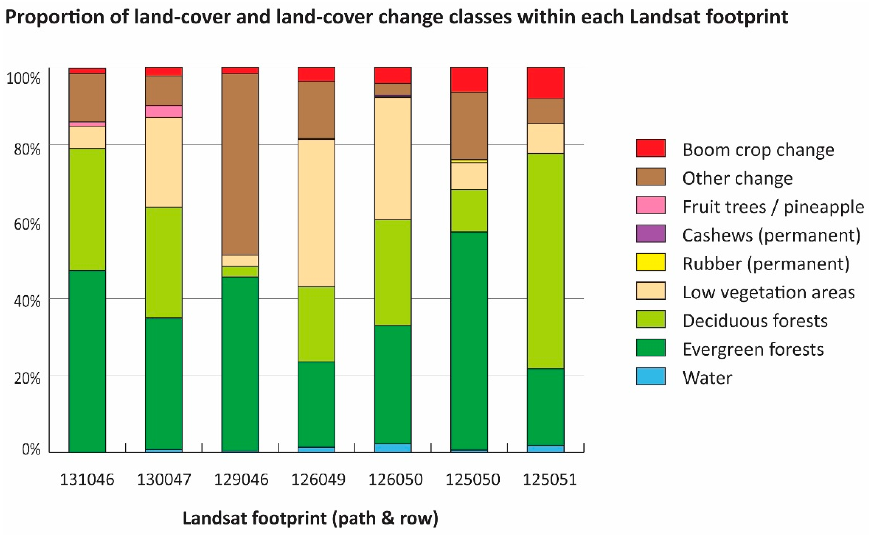
Figure 6.
Class separability of two classes with unbalanced samples in a two-dimensional feature space. (A) classes that cannot be separated; (B) classes with limited separability; and (C) separable classes after Burges [68] and Huang et al. [56].

Figure 7.
Expansion of boom crops between 2000 and 2014 mapped for three selected footprints (129046; 130047; 131046) in northern MSEA (Laos, Myanmar, Thailand).
Figure 7.
Expansion of boom crops between 2000 and 2014 mapped for three selected footprints (129046; 130047; 131046) in northern MSEA (Laos, Myanmar, Thailand).

Figure 8.
Total land area converted to boom crops (in km2) for the full period (2000–2014). Change classes were grouped by crop type and footprint. Y-axis scale is the same for all crop types with the exception of “conversions to rubber” and “other change” (large areas were transformed).
Figure 8.
Total land area converted to boom crops (in km2) for the full period (2000–2014). Change classes were grouped by crop type and footprint. Y-axis scale is the same for all crop types with the exception of “conversions to rubber” and “other change” (large areas were transformed).

Figure 9.
Expansion of boom crops between 2000 and 2014 mapped for four selected footprints (125050; 125051; 126049; 126050) in southern MSEA (Cambodia, Laos, Thailand, Vietnam).
Figure 9.
Expansion of boom crops between 2000 and 2014 mapped for four selected footprints (125050; 125051; 126049; 126050) in southern MSEA (Cambodia, Laos, Thailand, Vietnam).

Figure 10.
Conversion to rubber by year and conversion type in Stung Treng Province, Cambodia. Polygons with black borders are economic land concessions granted by the government of Cambodia for plantation crops.
Figure 10.
Conversion to rubber by year and conversion type in Stung Treng Province, Cambodia. Polygons with black borders are economic land concessions granted by the government of Cambodia for plantation crops.

Figure 11.
Conversions to rubber by year and conversion type in Thailand.

Figure 12.
Conversions to cashews between 2000 and 2008, Ratanakiri Province, Cambodia.


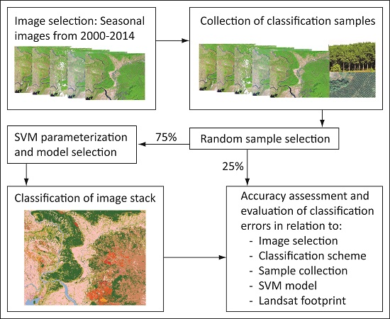
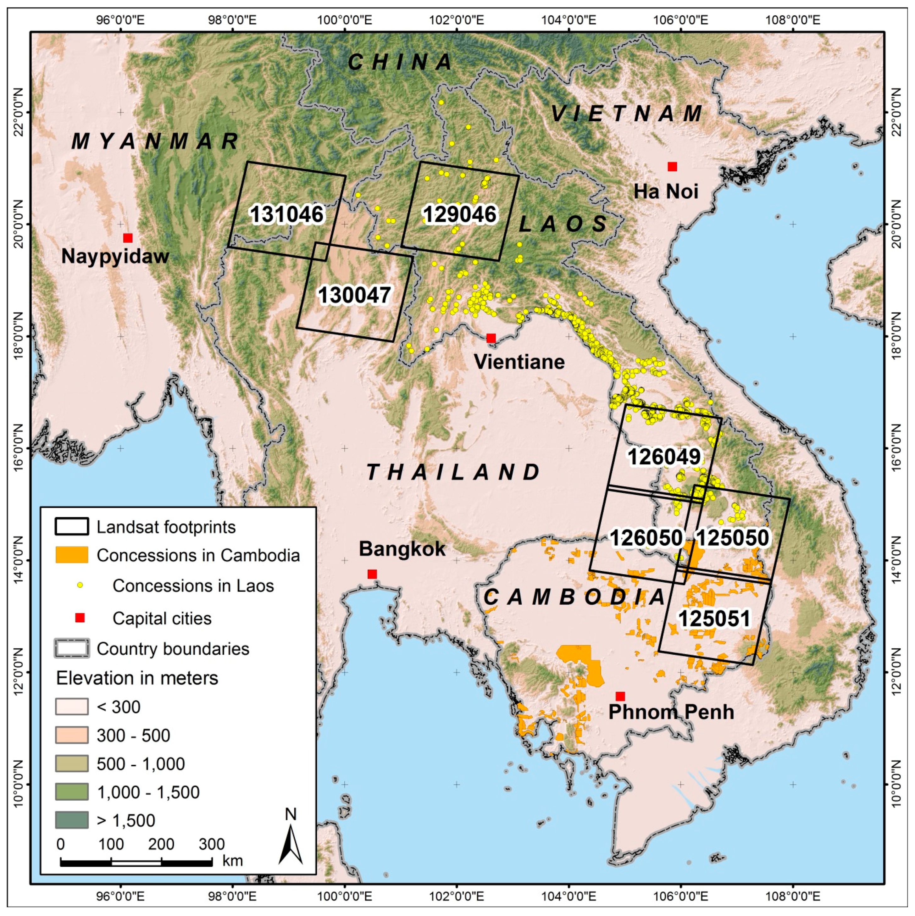
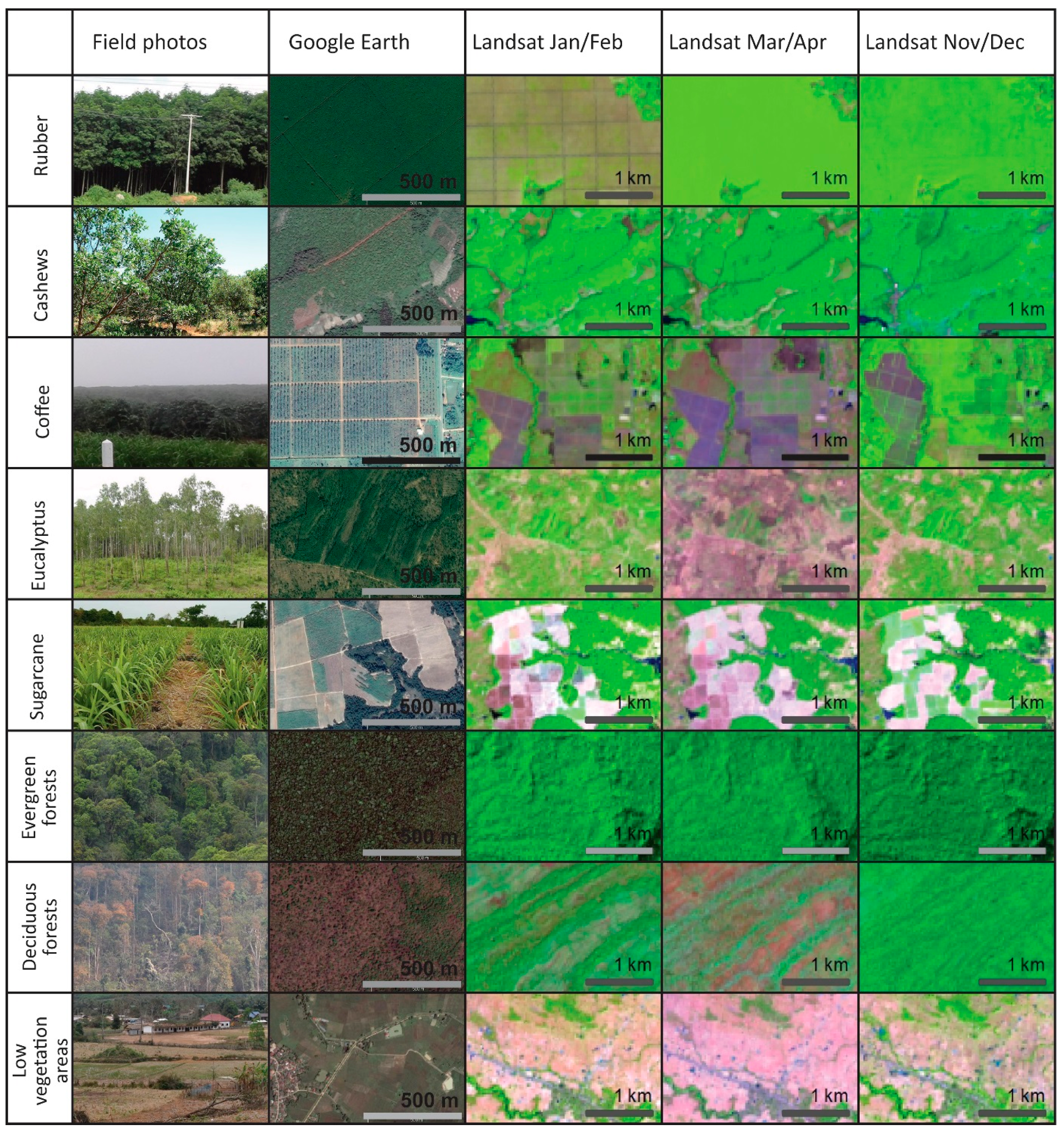
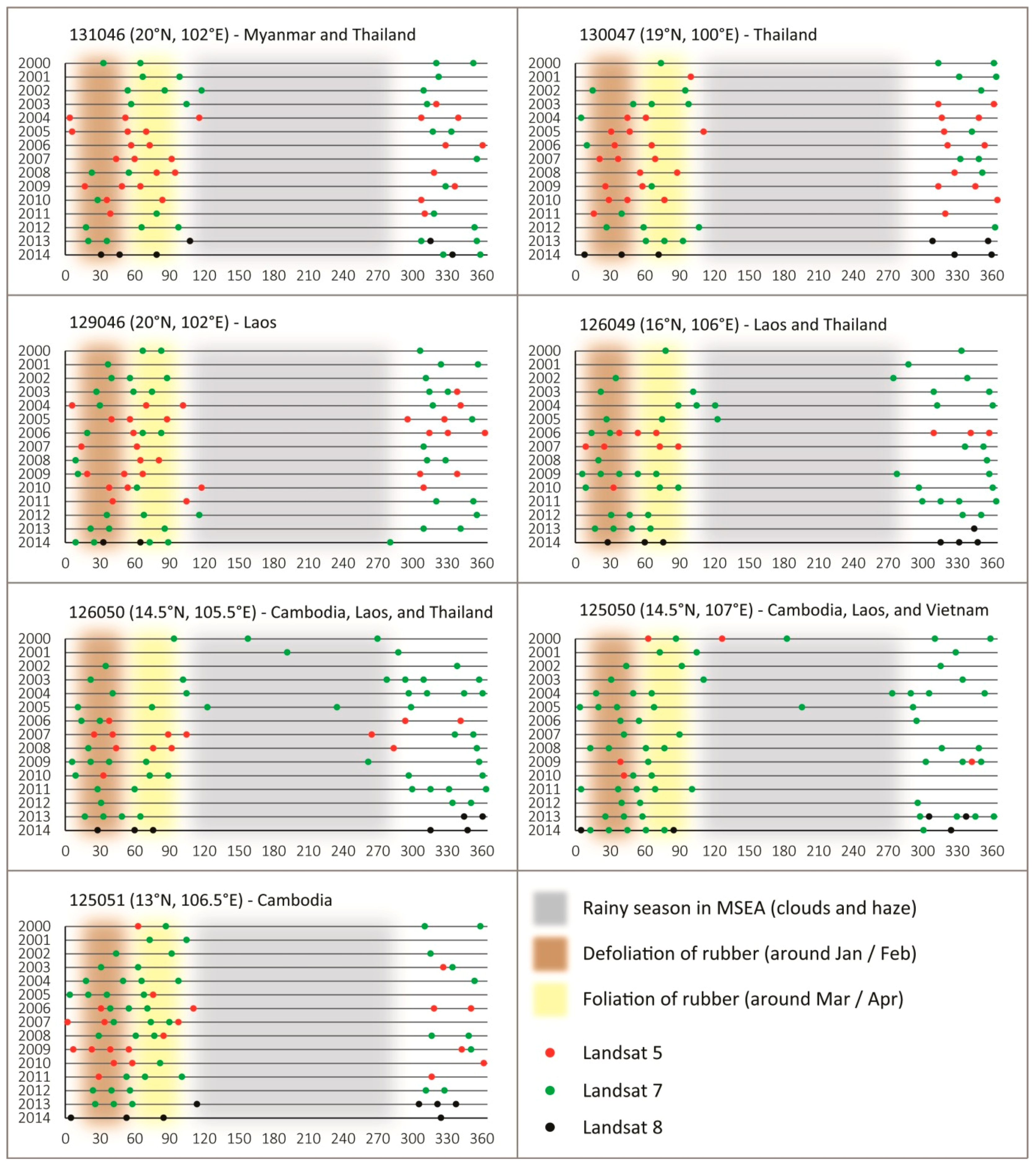
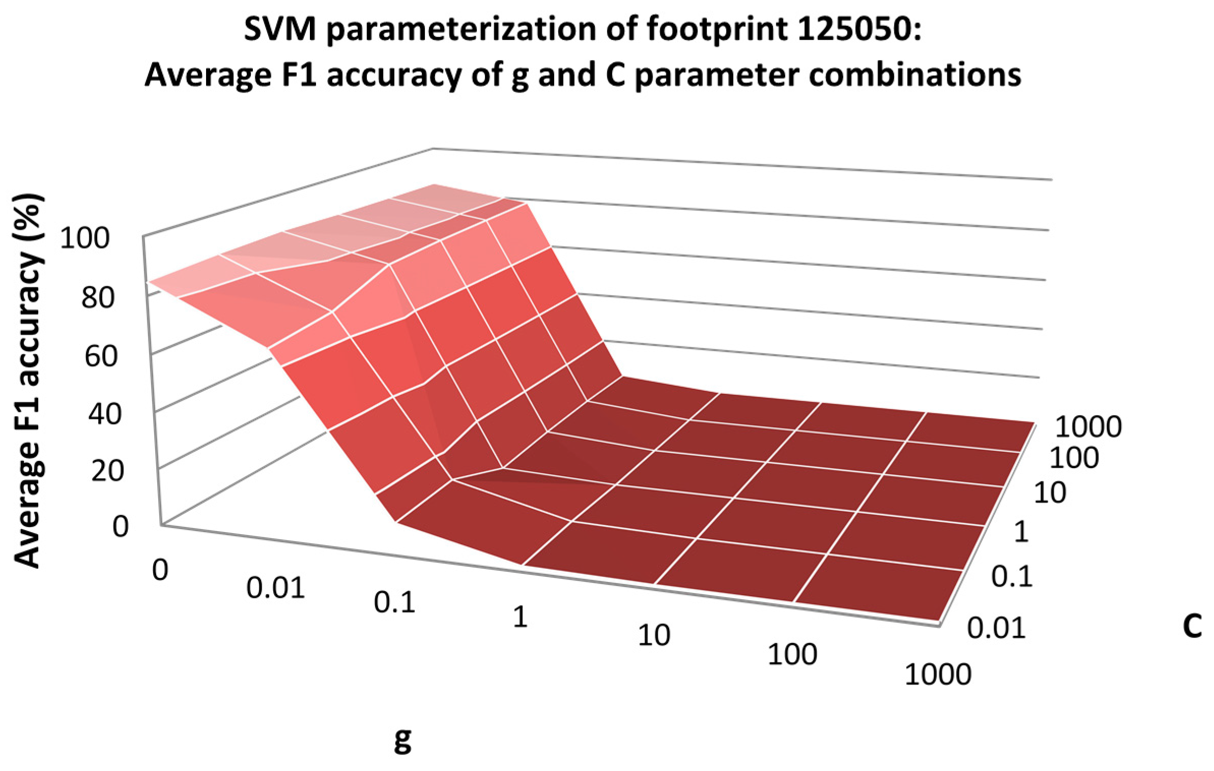
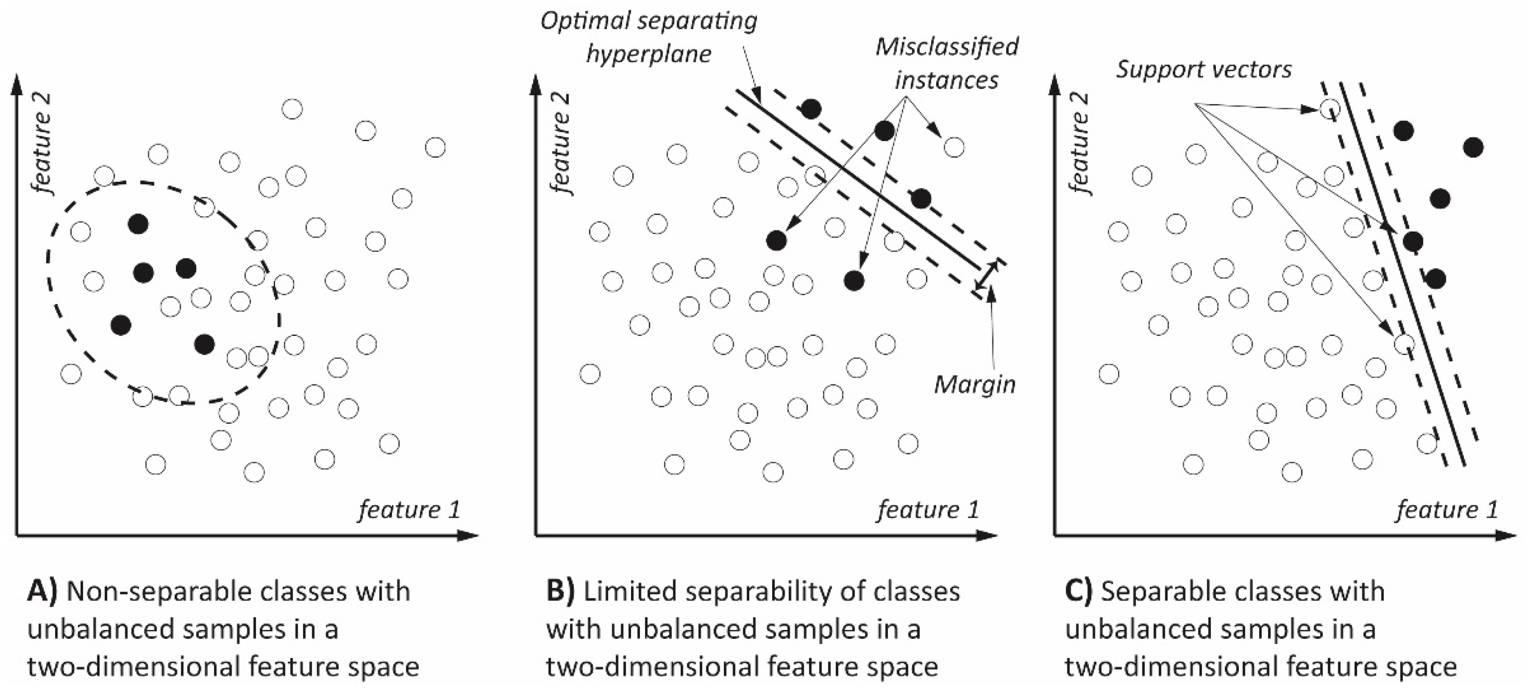
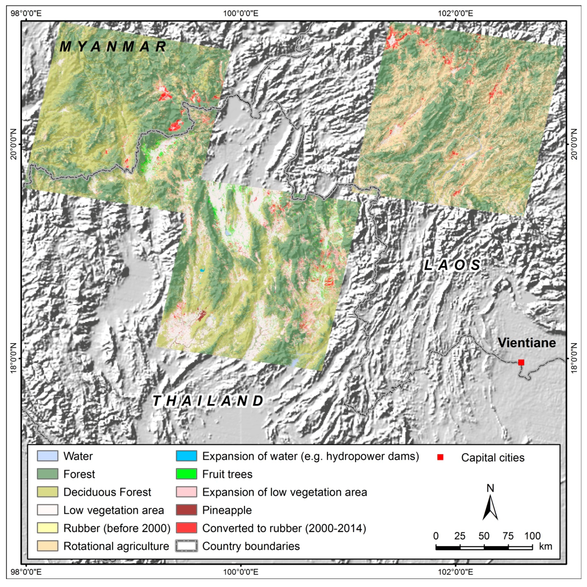
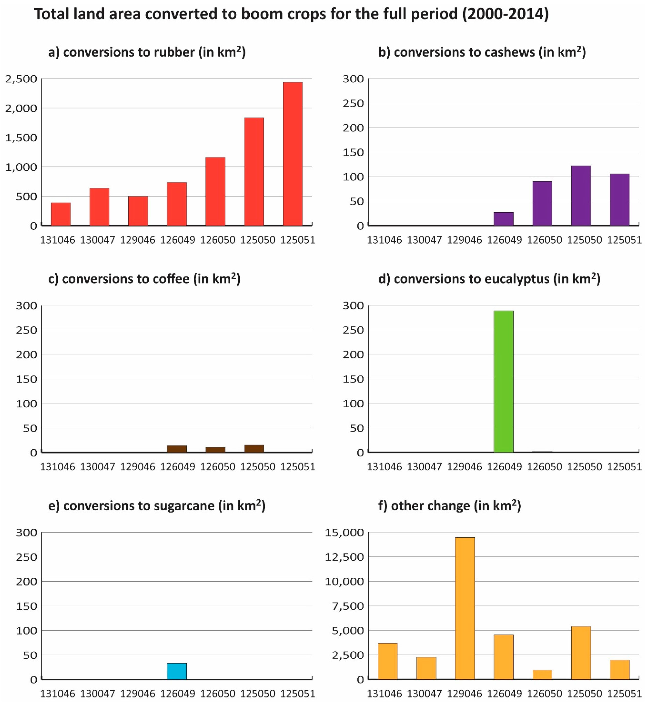
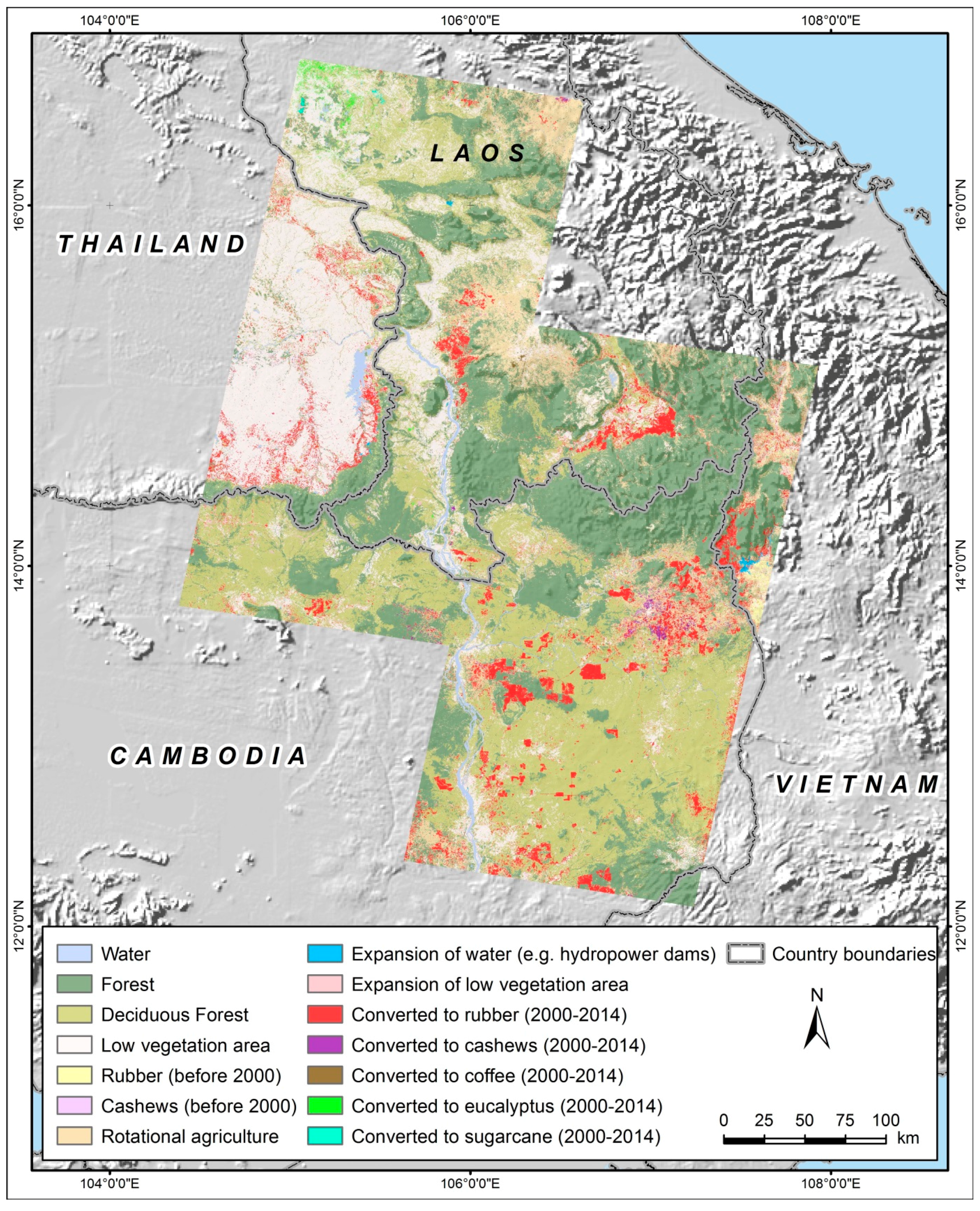
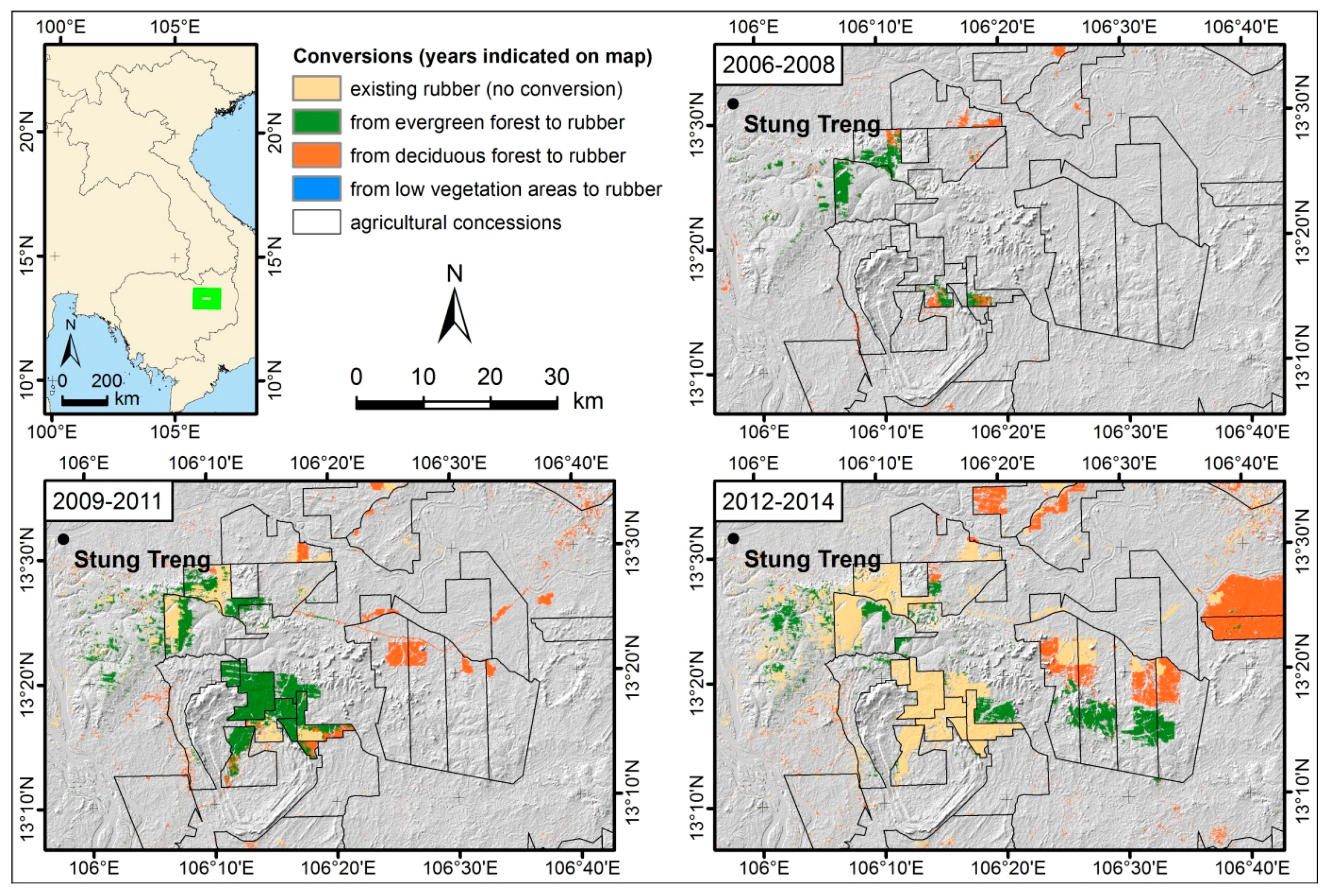
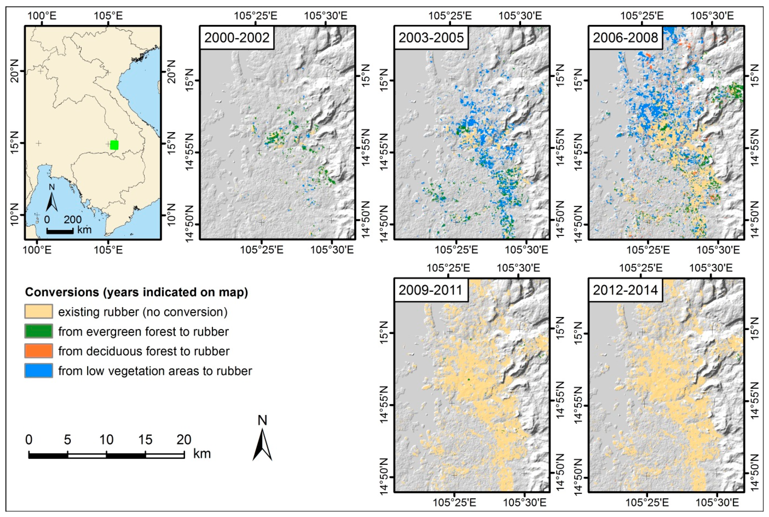
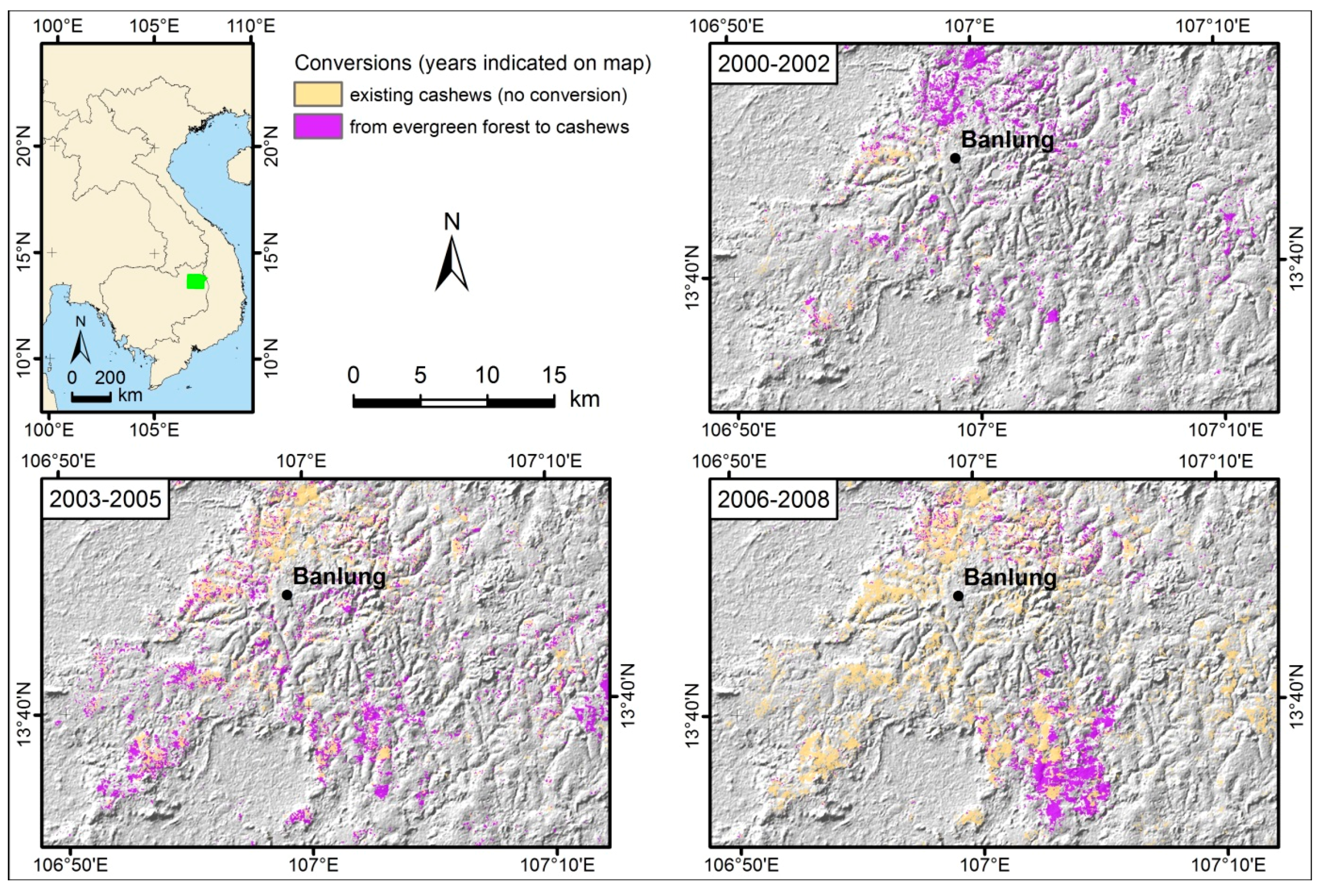
Table 1.
Land use and land cover change characteristics for the seven footprints in Mainland Southeast Asia.
Table 1.
Land use and land cover change characteristics for the seven footprints in Mainland Southeast Asia.
| Landsat Footprint | Countries | Primary Land Use/Land Cover Types | Primary Boom Crops |
|---|---|---|---|
| 131046 | Myanmar, Thailand | Evergreen and deciduous forests, low vegetation areas with mainly agriculture (Thailand) | Rubber, fruit trees (Thailand) |
| 130047 | Thailand | Low vegetation areas with mainly agriculture, evergreen and deciduous forests | Rubber, fruit trees, pineapple |
| 129046 | Laos | Evergreen forests, cropland/fallow land mosaic (rotational agriculture) | Rubber |
| 126049 | Laos, Thailand | Low vegetation areas with mainly agriculture, evergreen and deciduous forests, cropland/fallow land mosaic (rotational agriculture, Laos) | Rubber, sugarcane, eucalyptus (Laos) |
| 126050 | Cambodia, Laos, Thailand | Low vegetation areas with mainly agriculture, evergreen and deciduous forests | Rubber, cashews, eucalyptus |
| 125050 | Cambodia, Laos, Vietnam | Evergreen and deciduous forests | Rubber, coffee (Laos), cashews (Cambodia) |
| 125051 | Cambodia | Evergreen and deciduous forests | Rubber, cashews |
Table 2.
Classification scheme including the land-cover and land-cover change classes for all Landsat footprints. This study focused on the classes highlighted in grey.
Table 2.
Classification scheme including the land-cover and land-cover change classes for all Landsat footprints. This study focused on the classes highlighted in grey.
| 2000–2002 | 2003–2005 | 2006–2008 | 2009–2011 | 2012–2014 | |
|---|---|---|---|---|---|
| No change | Water | ||||
| Evergreen forests (EF) | |||||
| Deciduous forests (DF) | |||||
| Low vegetation areas (LVA) | |||||
| Rubber | |||||
| Cashews | |||||
| Pineapple | |||||
| Orchards/fruit trees | |||||
| Boom crop change | Rubber from EF | Rubber from EF | Rubber from EF | Rubber from EF | Rubber from EF |
| Rubber from DF | Rubber from DF | Rubber from DF | Rubber from DF | Rubber from DF | |
| Rubber from LVA | Rubber from LVA | Rubber from LVA | Rubber from LVA | Rubber from LVA | |
| Cashews from EF | Cashews from EF | Cashews from EF | Cashews from EF | Cashews from EF | |
| Cashews from DF | Cashews from DF | Cashews from DF | Cashews from DF | Cashews from DF | |
| Cashews from LVA | Cashews from LVA | Cashews from LVA | Cashews from LVA | Cashews from LVA | |
| Coffee from EF | Coffee from EF | Coffee from EF | Coffee from EF | Coffee from EF | |
| Coffee from DF | Coffee from DF | Coffee from DF | Coffee from DF | Coffee from DF | |
| Coffee from LVA | Coffee from LVA | Coffee from LVA | Coffee from LVA | Coffee from LVA | |
| Eucalyptus from EF | Eucalyptus from EF | Eucalyptus from EF | Eucalyptus from EF | Eucalyptus from EF | |
| Eucalyptus from DF | Eucalyptus from DF | Eucalyptus from DF | Eucalyptus from DF | Eucalyptus from DF | |
| Eucalyptus from LVA | Eucalyptus from LVA | Eucalyptus from LVA | Eucalyptus from LVA | Eucalyptus from LVA | |
| Sugarcane from EF | Sugarcane from EF | Sugarcane from EF | Sugarcane from EF | Sugarcane from EF | |
| Sugarcane from DF | Sugarcane from DF | Sugarcane from DF | Sugarcane from DF | Sugarcane from DF | |
| Sugarcane from LVA | Sugarcane from LVA | Sugarcane from LVA | Sugarcane from LVA | Sugarcane from LVA | |
| Other change | Rotational agriculture | ||||
| Expansion of low vegetation areas | |||||
| New hydropower dams | |||||
Table 3.
Parameterization of the Support Vector Machines (SVM) classifier illustrating the best parameter setting for each footprint, overall accuracy, the averaged F1 measure, and the number of bands, classes, and training samples.
Table 3.
Parameterization of the Support Vector Machines (SVM) classifier illustrating the best parameter setting for each footprint, overall accuracy, the averaged F1 measure, and the number of bands, classes, and training samples.
| Footprint | Overall Accuracy (%) | F1 Measure (%) | C | g | Number of Bands | Number of Classes | Number of Samples |
|---|---|---|---|---|---|---|---|
| 131046 | 86.6 | 86 | 1000 | 0 | 408 | 19 | 1816 |
| 130047 | 89.6 | 84.3 | 0.1 | 0 | 391 | 19 | 2389 |
| 129046 | 84.7 | 86 | 0.01 | 0 | 446 | 12 | 2805 |
| 126049 | 87.8 | 82.4 | 0.01 | 0 | 415 | 31 | 3108 |
| 126050 | 89.9 | 85.6 | 0.1 | 0 | 419 | 29 | 3173 |
| 125050 | 85.4 | 84.7 | 1 | 0 | 365 | 23 | 2316 |
| 125051 | 93.3 | 91.4 | 0.1 | 0 | 440 | 19 | 3528 |
Table 4.
User’s and producer’s accuracies for the three groups of classes: no change, boom crop change, other change in each footprint.
Table 4.
User’s and producer’s accuracies for the three groups of classes: no change, boom crop change, other change in each footprint.
| Footprint | No Change | Boom Crop Change | Other Change | |||
|---|---|---|---|---|---|---|
| UA (%) | PA (%) | UA (%) | PA (%) | UA (%) | PA (%) | |
| 131046 | 91.4 | 90.7 | 85.7 | 85.0 | 64.9 | 68.5 |
| 130047 | 92.7 | 96.6 | 84.0 | 84.0 | 91.3 | 55.3 |
| 129046 | 88.4 | 85.8 | 84.1 | 81.1 | 81.9 | 87.1 |
| 126049 | 92.3 | 92.8 | 89.0 | 85.1 | 69.1 | 80.7 |
| 126050 | 95.0 | 96.8 | 83.8 | 81.9 | 85.1 | 83.8 |
| 125050 | 85.9 | 87.1 | 87.3 | 89.0 | 73.2 | 63.1 |
| 125051 | 90.2 | 92.7 | 95.0 | 95.9 | 82.4 | 60.9 |
© 2017 by the authors. Licensee MDPI, Basel, Switzerland. This article is an open access article distributed under the terms and conditions of the Creative Commons Attribution (CC BY) license (http://creativecommons.org/licenses/by/4.0/).
Share and Cite
MDPI and ACS Style
Hurni, K.; Schneider, A.; Heinimann, A.; Nong, D.H.; Fox, J. Mapping the Expansion of Boom Crops in Mainland Southeast Asia Using Dense Time Stacks of Landsat Data. Remote Sens. 2017, 9, 320. https://doi.org/10.3390/rs9040320
AMA Style
Hurni K, Schneider A, Heinimann A, Nong DH, Fox J. Mapping the Expansion of Boom Crops in Mainland Southeast Asia Using Dense Time Stacks of Landsat Data. Remote Sensing. 2017; 9(4):320. https://doi.org/10.3390/rs9040320
Chicago/Turabian StyleHurni, Kaspar, Annemarie Schneider, Andreas Heinimann, Duong H. Nong, and Jefferson Fox. 2017. "Mapping the Expansion of Boom Crops in Mainland Southeast Asia Using Dense Time Stacks of Landsat Data" Remote Sensing 9, no. 4: 320. https://doi.org/10.3390/rs9040320
Note that from the first issue of 2016, this journal uses article numbers instead of page numbers. See further details here.