Mapping Urban Bare Land Automatically from Landsat Imagery with a Simple Index

Abstract

In recent years, hundreds of Earth observation satellites have been launched to collect massive amounts of remote sensing images. However, the considerable cost and time to process the significant amount of data have become the greatest obstacle between data and knowledge. In order to accelerate the transformation from remote sensing images to urban thematic maps, a strategy to map the bare land automatically from Landsat imagery was developed and assessed in this study. First, a normalized difference bare land index (NBLI) was presented to maximally differentiate bare land from other land types in Wuhan City, China. Then, an unsupervised classifier was employed to extract the bare land from the NBLI image without training samples or self-assigned thresholds. Experimental results showed good performance on overall accuracy (92%), kappa coefficient (0.84), area ratio (1.1321), and match rate (83.96%), respectively. Results in multiple years disclosed that bare lands in the study site gradually moved from inner loops to the outer loops since 2007, in two main directions. This study demonstrated that the proposed method was an accurate and reliable option to extract the bare land, which led to a promising approach to mapping urban land use/land cover (LULC) automatically with simple indices.

1. Introduction

In this study, bare land indicates land not covered by vegetation, water, buildings, or roads, on the Earth’s surface. It is one of the most important and typical land covers all over the world. For a city under rapid development, the spatial-temporal change of the bare land is commonly recognized as the indicator of humans’ endeavors to rebuild or expand a city [1,2]. In Chinese megacities, numerous bare land pieces emerged along with urbanization processes, which cast irreversible impacts on the urban environment, such as air pollution and soil loss.

In recent decades, most researchers have been inclined to map urban land use and land cover (LULC) with supervised classification methods [3,4]. However, selecting samples interactively needs a considerable amount of time, labor, and expert knowledge [5]. This becomes even worse when mapping urban LULC in multiple years, as training samples have to be collected for each year. For this reason, a classifier designed for one time use often cannot be directly implemented at a different time [6,7]. Consequently, it is difficult to analyze LULC changes routinely in a large number of time series.

A remote sensing index is a simple and effective way to highlight a specific land cover. For example, vegetation indices such as the normalized difference vegetation index (NDVI) [8] and enhanced vegetation index (EVI) [9] have been developed to detect vegetation greenness, and water indices such as the normalized difference water index (NDWI) [10] and the modified NDWI (MNDWI) [11] have been used to extract water properties in many applications. To extract specific land cover from an index image, a suitable threshold is critical because it has significant affects the mapping accuracy [12].

However, it is difficult to visually differentiate bare land and the built-up areas in one image due to their high complexity and similarity of spectral response patterns, especially in a mixture of pixels with heterogeneous objects [13,14,15]. For example, in the normalized difference built-up index (NDBI) [13], index-based built-up index (IBI) [16], and urban index (UI) [17] images, the difference between the bare land and built-up areas is limited. Therefore, these indices result in high uncertainties when assigning the threshold to identify bare land.

Recently, several indices have been presented to better distinguish the bare land, including the normalized difference bareness index (NDBaI) [1] and enhanced built-up and bareness index (EBBI) [18]. However, both indices have to specify the threshold interactively to extract the bare land. It is commonly believed that assigning a suitable threshold value is difficult [19,20,21]. A high threshold value often causes underestimation of bare land, while a low value results in overestimation. Repetitive experiments and comparisons are always needed to define a suitable threshold.

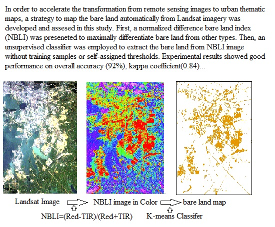
This study aimed to find a strategy to map the bare land automatically from Landsat imagery without training samples or self-defined thresholds. First, a novel bare land index was developed to distinguish the bare land from all other classes. Then an unsupervised classifier was adopted to map it with default settings. Results were assessed with ground truth samples. With this strategy, then, the spatial-temporal change of the bare land from 2007 to 2013 were mapped and analyzed. Finally, potential applications and prospects of the proposed strategy were discussed.

2. Materials

2.1. Study Site

The study is conducted in Wuhan City, the capital of Hubei province and the largest megacity in Central China (Figure 1a,b). Wuhan is located at 29°58′–31°22′N and 113°41′–115°05′E, and occupies a land area of 8494.41 square kilometers (3279.71 sq mi). Wuhan is known as the “Chicago of China” [22,23] due to its critical role in inland transportation. The city’s climate is humid subtropical, with plentiful rainfall and distinctive seasons. The mean temperature has the lowest 3.7 °C in January, and the highest 28.7 °C in July. Annual precipitation totals 1315 millimeters (51.8 in), mainly from May to July [24]. Most of the city has flat terrain decorated with hills and a great number of water bodies.

As one of the largest developing city in China, Wuhan is undergoing the most dramatic expansion in its history. Since 2007, the city has more than 5000 construction fields each year, and many of them last more than one year [25]. On one hand, the rapid expansion brings great benefits to citizens, such as job opportunities, convenient transportation, beautiful views and modern residence environments. On the other hand, it induces serious air pollution (i.e., smog), water pollution, and soil loss to the city [26,27].

In the city, the built-up lands are generally located within the 2nd loops, and areas under development are often distributed beyond the 3rd loop (Figure 1c).

2.2. Datasets

Landsat time-series images covering the Wuhan City (Path: 123, Row: 39) since 2007 were collected with special consideration for cloud, phenology and dryness of ground. As shown in

Table 1. Landsat images used in this research.

Captured Date	Scene ID	Sensor	Bands	Spatial Resolution (m)	Cloud Amount (%)
31 July 2007	LT51230392007212BJC01	TM	7	30	0.01
6 September 2009	LT51230392009249BJC00	TM	7	30	0.06
8 June 2011	LT51230392011159BKT00	TM	7	30	0
16 August 2013	LC81230392013228LGN00	OLI&TIRS	11	30	13.88

, images in green season of 2007, 2009, 2011, and 2013 are used in this study. Landsat thermal infrared (TIR) bands were rescaled to 30 m prior to building an index image.

A sample of Landsat TM image on 31 July 2007 is shown in Figure 2. Many large pieces of bare lands distribute (in light yellow tone) around built-up areas and lakes, illustrating the ongoing urban expansion. Atmospheric correction was implemented by the FLAASH model in ENVI 5.1 (provided by Harris Corporation in Melbourne, FL, USA) with the Landsat sensor response functions, metadata of the Landsat images, and meteorological data at the Wuhan station. The FLAASH model could effectively correct wavelengths in the visible through near-infrared and shortwave infrared regions incorporating the MODTRAN radiation transfer code. The digital numbers of the Landsat image were converted to apparent surface reflectance through this process.

The basic map, climate and environment data of the city were collected from Wuhan Municipal Environmental Protection Bureau. The related social, commercial and transportation data came from Wuhan Statistical Yearbook.

Validation points came from an independent set of very high resolution (VHR) imagery covering the study site, including IKONOS scenes in 2007 and 2013, Worldview scenes in 2009 and Quick bird scenes in 2011. Two hundreds of samples for the bare land and “the other” land types, respectively, were randomly interpreted from VHR images. These samples were used the confusion matrix to assess the mapping accuracy.

3. Methods

3.1. The Normalized Difference Bare Land Index

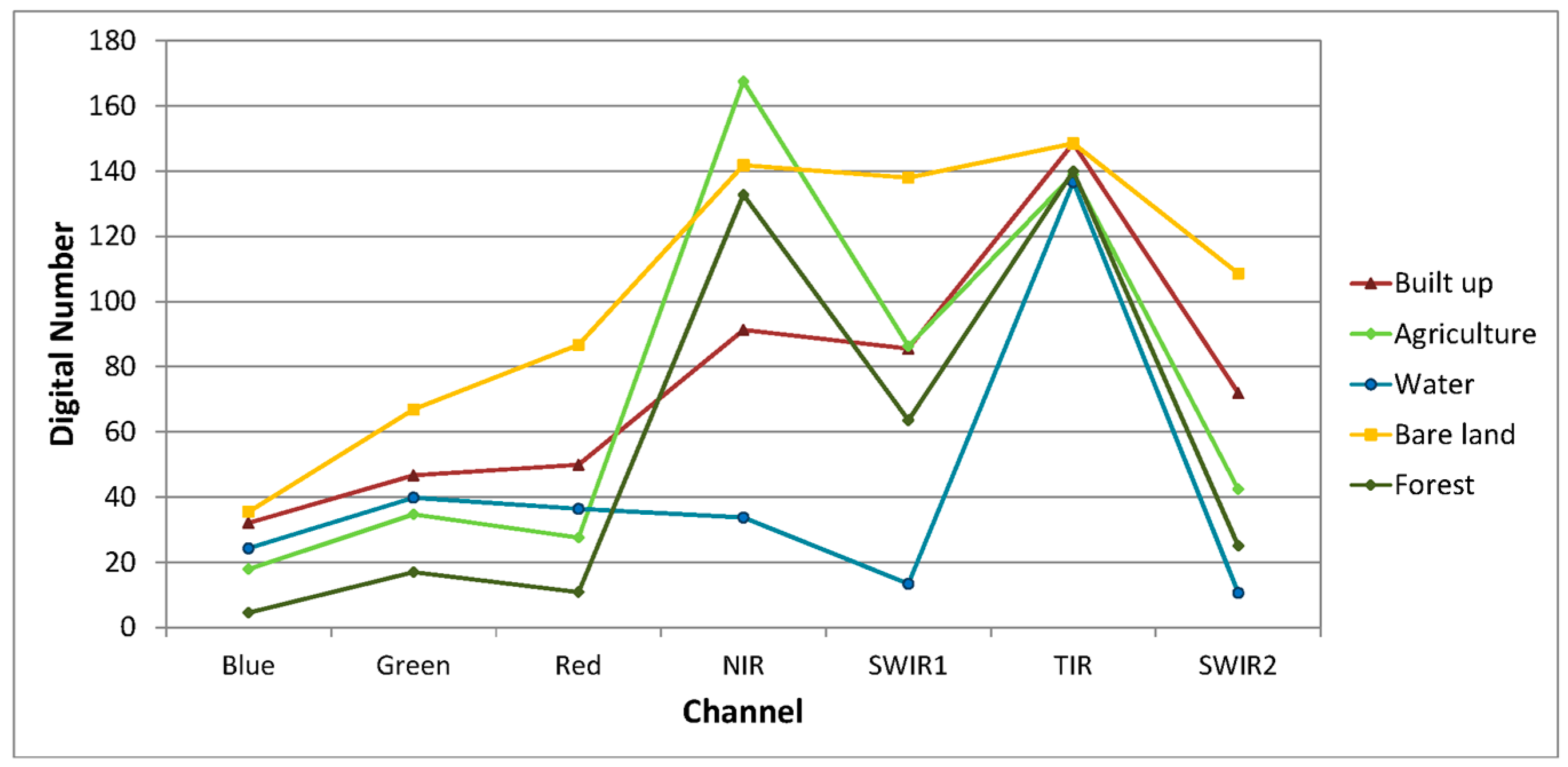
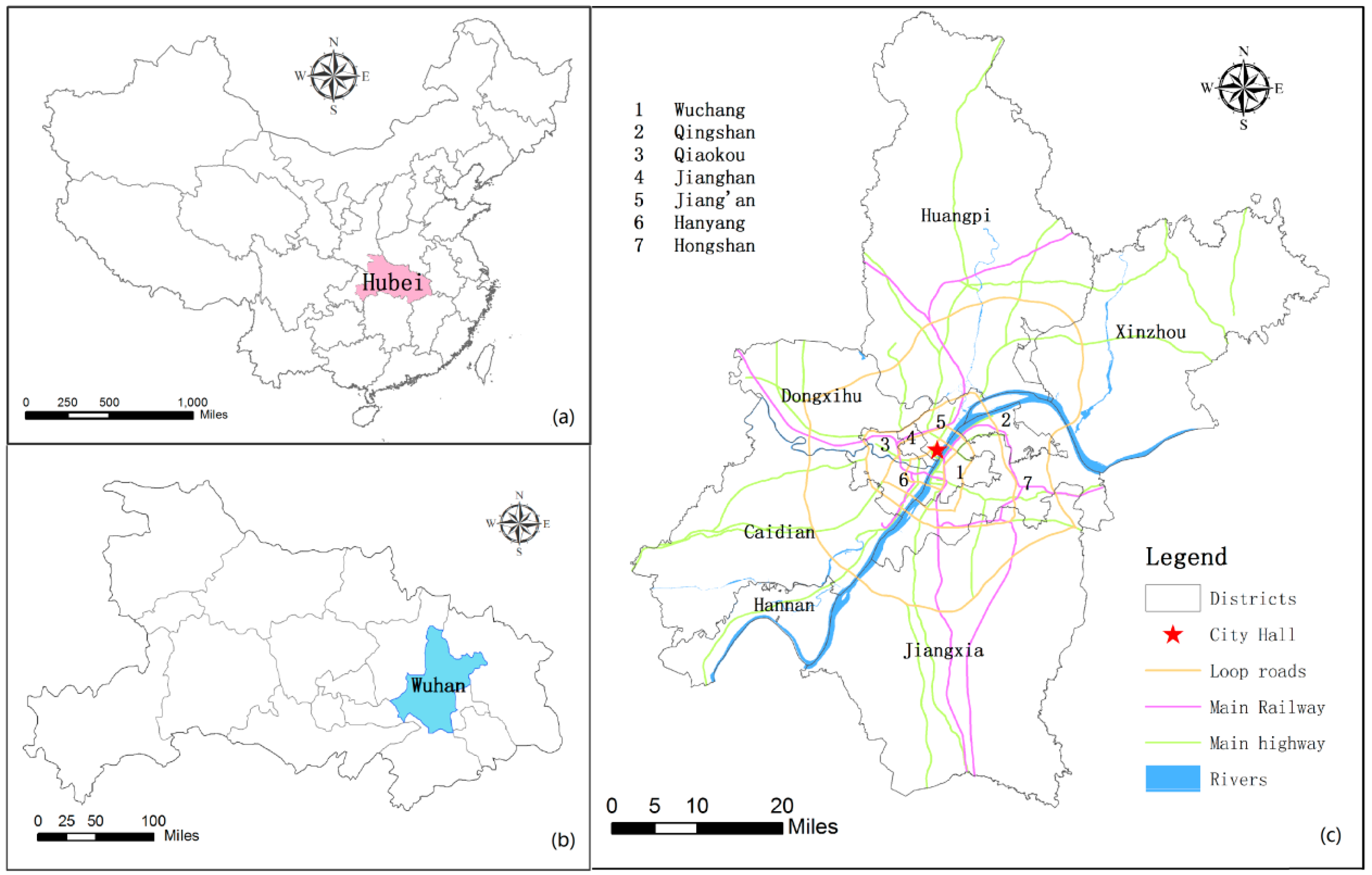
In this study, land covers within the city were simply divided into five typical classes, i.e., the built up, bare land, water, forest, and agriculture. Here, agriculture is actually the mixture of cropland, grassland, and other vegetation land except the forest. As a city in the Jianghan Plain, cropland is the main land cover in the city. Two hundreds samples for each class were selected manually to depict the spectral profiles.

As shown in Figure 3, the difference between the bare land and all others is apparent at the SWIR1 band (band 5 in TM) and red band (band 3 in TM). Especially, the SWIR1 band exhibits a high level of contrast to the water, which makes it widely used in bare land mapping [1,18]. However, digital numbers (DN) of agriculture are the closest to the bare land at SWIR1. Considering that agriculture is actually the mixture of several land cover types, its variation range could be large. Thus, the overlap between the bare land and agriculture may exist at SWIR.

The built-up and bare land show similar tendencies from the band 4 (NIR) to band 5 (SWIR1), which are different from all others. Some indices utilize this feature to highlight the built-up areas [16,17], where the bare land is not considered as a standalone land cover type.

The red band (band 3 in TM) also reveals high contrast between the bare land and others with its much higher DN values. Meanwhile, it is clear that all classes have similar DN values at TIR band (Band 6 in TM). Thus, the difference between the two bands could help distinguish the bare land from other classes. In order to restrict the value range, we developed a normalized difference bare land index (NBLI) as the following formula:

$$\mathrm{NBLI}=\left(\mathrm{Red}-\mathrm{TIR}\right)/\left(\mathrm{Red}+\mathrm{TIR}\right)$$

(1)

When dealing with Landsat 8 image, band 4 (red) and band 10 (TIR) can be utilized to build the NBLI.

3.2. Comparison with Related Indices

To verify the performance of our proposed index, experiments on other urban-related indices were carried out in a comparison analysis, including the normalized difference built-up index (NDBI) [13], Urban Index (UI) [17], index-based built-up index (ibi) [16], normalized difference bare land index (NDBaI) [1], and enhanced built-up and bare land index (EBBI) [18]. All of these indices have been developed to map urban environments. The NDBI used TM4 and TM5 and was applied in extracting urban areas of Nanjing City, China [13]. The UI used Landsat TM band 7 and band 4, exploiting an inverse relationship between the brightness of urban areas in the near infrared (0.76–0.90 µm) and mid-infrared (2.08–2.35 µm) spectral regions [17]. The IBI made use of three indices, including the MNDWI, NDBI, and the soil-adjusted vegetation index (SAVI) [19]. The subtraction of the SAVI band and the MNDWI band from the NDBI band results in positive values for built-up land pixels only. The NDBaI distinguished the bare land with Landsat band 5 (SWIR1) and band 6 (TIR) [1]. The EBBI mapped the built-up and bare land at the same time, with the band NIR, SWIR1, and TIR (Landsat ETM+ bands 4, 5, and 6) [18].

The formulas of these related indices are as below:

$$\mathrm{IBI}=\frac{2\mathrm{SWIR}1/\left(\mathrm{SWIR}1+\mathrm{NIR}\right)-\left[\mathrm{NIR}/\left(\mathrm{NIR}+\mathrm{Red}\right)+\mathrm{Green}/\left(\mathrm{Green}+\mathrm{SWIR}1\right)\right]}{2\mathrm{SWIR}1/\left(\mathrm{SWIR}1+\mathrm{NIR}\right)+\left[\mathrm{NIR}/\left(\mathrm{NIR}+\mathrm{Red}\right)+\mathrm{Green}/\left(\mathrm{Green}+\mathrm{SWIR}1\right)\right]}$$

(2)

$$\mathrm{NDBI}=\left(\mathrm{SWIR}1-\mathrm{NIR}\right)/\left(\mathrm{SWIR}1-\mathrm{NIR}\right)$$

(3)

$$\mathrm{UI}=\left(\mathrm{SWIR}2-\mathrm{NIR}\right)/\left(\mathrm{SWIR}2+\mathrm{NIR}\right)$$

(4)

$$\mathrm{NDBaI}=\left(\mathrm{SWIR}1-\mathrm{TIR}\right)/\left(\mathrm{SWIR}1+\mathrm{TIR}\right)$$

(5)

$$\mathrm{EBBI}=\left(\mathrm{SWIR}1-\mathrm{NIR}\right)/\left(10\sqrt{\mathrm{SWIR}1+\mathrm{TIR}}\right)$$

(6)

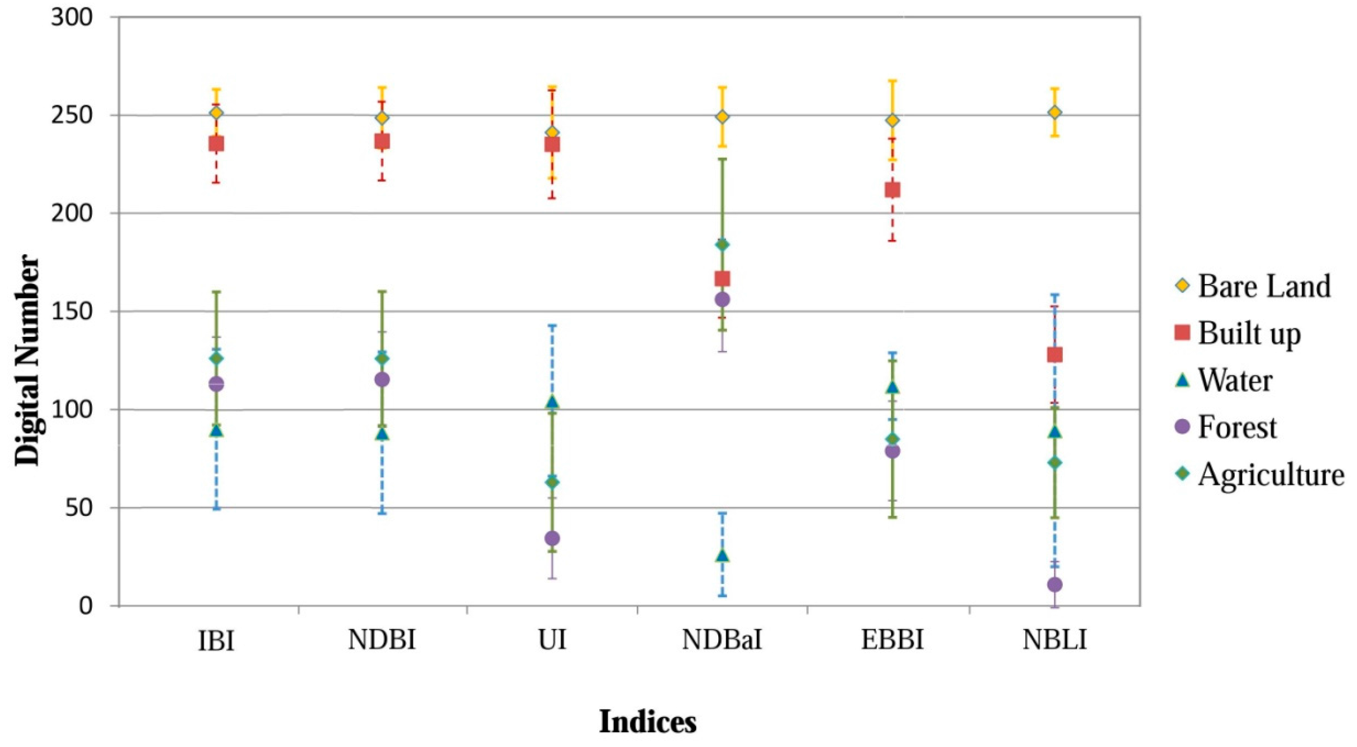
In order to test their abilities to distinguish the bare land from other classes, samples of typical land covers were selected from these index images, and then statistics of the land covers in different index images were presented (Figure 4).

In Figure 4, the mean values of the bare land in all index images are close to 255, showing that all indices are able to fairly highlight the bare land. However, in the first three index images, i.e., IBI, NDBI, and UI, both statistics (i.e., the mean and standard deviation) of the bare land are very close to those of the built-up. For the NDBaI, the distance between the agriculture and the bare land is not far enough for separating them clearly. They actually overlap at 95% confidence interval (two times the standard deviation). For the EBBI, the distance between the bare land and built-up areas increases slightly, however, the overlap between them is still serious. The NBLI proposed in this study maximally separates the bare land from others, which makes it easier to specify the threshold for extracting bare land from a Landsat image. It is also noticed in Figure 4 that the distributions of bare land and water may slightly overlap at a 95% confidence interval. To reduce the potential classification errors, water bodies have to be removed before extracting the bare land.

3.3. Mapping the Bare Land Automatically with NBLI

Traditionally, assigning the threshold for extracting a specified land cover often costs considerable time and labor sources. The apparently different values of NBLI in Figure 4 trigger our motivation to test if it is possible to assign the threshold automatically. In order to test the possibility, a common unsupervised classifier, the k-means function embedded in ENVI 5.1 with default settings, is employed to assign the threshold for extracting the bare land from the index image. The flowchart of the proposed method is shown in Figure 5 and discussed below.

After testing several typical water indices with the method similar to that in Section 3.2, the MNDWI is selected to distinguish the water body. Then, the unsupervised classifier, k-means is employed to specify the threshold for extracting the water body automatically.

The extracted water bodies serve as a mask layer to remove water bodies in the NBLI index image. Then, the k-means classifier is implemented to divide the index image into several classes. As demonstrated in Figure 4, pixels with the highest values are automatically classified as the bare land, and all others are combined into “the other” class.

3.4. Accuracy Assessment

Two quantitative methods are employed to assess the accuracies of the classification. First, the traditional confusion (error) matrix is employed with the validation sample samples. The overall accuracy is calculated as the ratio between the sum of the samples along the diagonal to the total number of validation samples. The Kappa coefficient of agreement is also derived from the confusion matrix.

Secondly, a traditional supervised classification was implemented with the validation samples in the support vector machine (SVM) classifier. Two indicators are developed to investigate the differences between the automatic mapping result and the supervised classification result, i.e., the area ratio ($R_a$) and match rate ($R_m$). Their formulas are shown below:

$$R_a=B_a/B_r$$

(7)

$$R_m=(B_a{\displaystyle \cap }{B}_r)/B_r\mathrm{or}{R}_m=(B_a{\displaystyle \cap }{B}_r)/B_a$$

(8)

where $B_a$ indicates the bare land in the automatic mapping result, and $B_r$ represents the bare land in the supervised classification result.

4. Results

4.1. Index Images

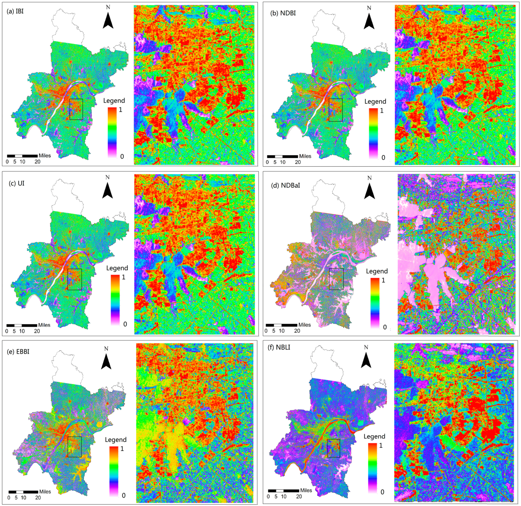
All indices applied in this study, including the IBI, NDBI, UI, NDBaI, EBBI, and NBLI, are extracted from the TM scenes. Figure 6 demonstrates their visual differences in Wuhan City on 31 July 2007.

In the first three images (Figure 6a–c), the bare lands are confused with built up areas. In the NDBaI image (Figure 6d), the difference between the bare land and built-up areas becomes larger. However, the difference between the bare land and agriculture is very small. In the EBBI image (Figure 6e), the difference between the bare land and built-up areas is also not large enough to reach satisfactory classification. In the NBLI image (Figure 6f), the difference between the bare land and all others (except some water bodies) is so clear that the bare land can be interpreted easily. The unique problem is that some water bodies with large amount of suspended soil may have similar value with the bare land, such as the Yangzi River. In this case, it is necessary to remove the water body before mapping the bare land.

4.2. Mapping the Bare Land

As the difference between the bare land and built-up is small in the IBI, NDBI, and UI images, the unsupervised classifier cannot produce meaningful results from these images. Thus, just the NDBaI, EBBI, and NBLI images were compared for extracting the bare land with the k-means classifier. Additionally, with the samples interpreted from VHR images, a supervised classification were carried out with a support vector machine (SVM). The results are shown in Figure 7 and

Table 2. Accuracy assessment.

	Overall Acc. (%)	Kappa Coefficient	Prod. Acc. (%)		User Acc. (%)		Comparison with the Reference
			Bare	Other	Bare	Other	Area Ratio	Match Rate (%)
NDBaI	85.45	71.00	76.00	94.90	93.71	79.81	3.77	74.65
EBBI	90.55	81.00	82.40	98.60	98.33	84.85	1.85	82.84
NBLI	92.00	84.00	84.20	99.80	99.76	86.33	1.13	83.96
SVM	96.75	93.50	94.00	99.50	99.47	94.31	-	-

.

Large areas of agriculture land are classified as bare lands in the NDBaI result (Figure 7a). The misclassification between the agriculture and bare land is high. In the EBBI result (Figure 7b), many built up areas (within the inner loops) are misclassified as bare lands. In the final NBLI result (Figure 7c), the distribution of bare lands is very similar to the supervised classification result in Figure 7f. These results in Figure 7 clearly illustrates that the bare land extracted from the NBLI image is the best result, when using an unsupervised classifier to specify the threshold.

Additionally, Figure 7d shows some water bodies, such as the Yangzi River, are misclassified as bare lands in the original NBLI result when water bodies are not removed. Thus, it is necessary to remove them from the NBLI image. Figure 7e presents water bodies extracted from the MNDWI image with the unsupervised k-means classifier. The distribution matches the visual interpretation very well, and the overall accuracy in the confusion matrix achieves 95%. This guarantees the accuracy level of the final result extracted from the water-masked NBLI image.

In Table 2, the NBLI result has the best overall accuracy, kappa coefficient, producer’s accuracy, and user’s accuracy. Especially, the area ratio of NBLI result is much lower than that of other indices, meaning that many fewer pixels of other classes are classified as the bare land in the result. With the first formula in Equation (8), the match rate reaches a good match, especially for the NBLI (83.96%). When using the second formula in Equation (8), the values become 19.78% (NDBaI), 44.73% (EBBI), and 74.30% (NBLI), respectively. These differences among the three methods become much higher, mainly due to great differences in area ratio. From all accuracy measures in the confusion matrix in Table 2, the NBLI result has the highest performance among the three indices.

Generally, all indicators show the NBLI result has much better performance, and could meet the requirements of most application. Therefore, mapping the bare land from the NBLI image with the automatic strategy, as proposed in this study, is feasible and reliable.

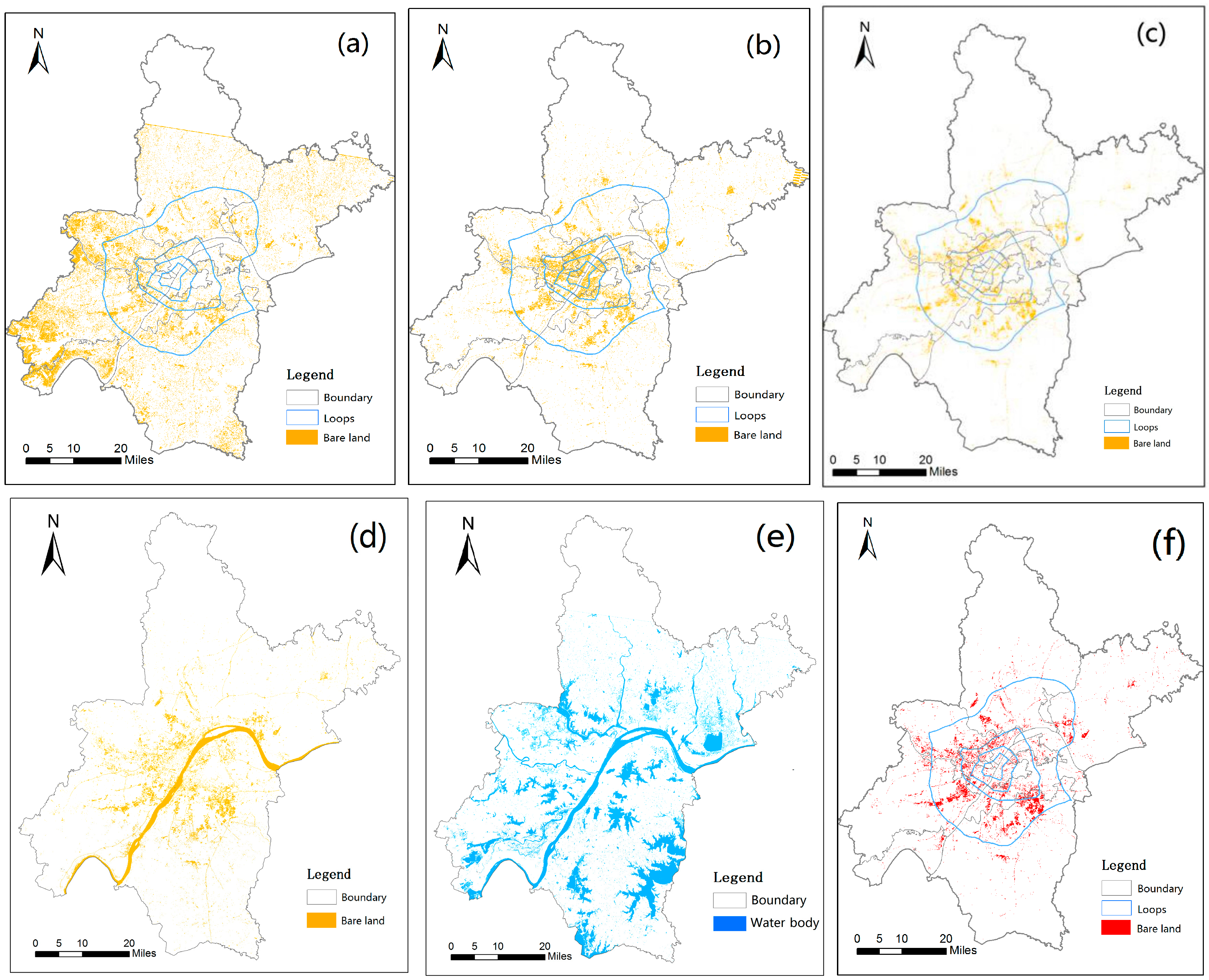
4.3. Mapping the Spatial-Temporal Change of the Bare Land

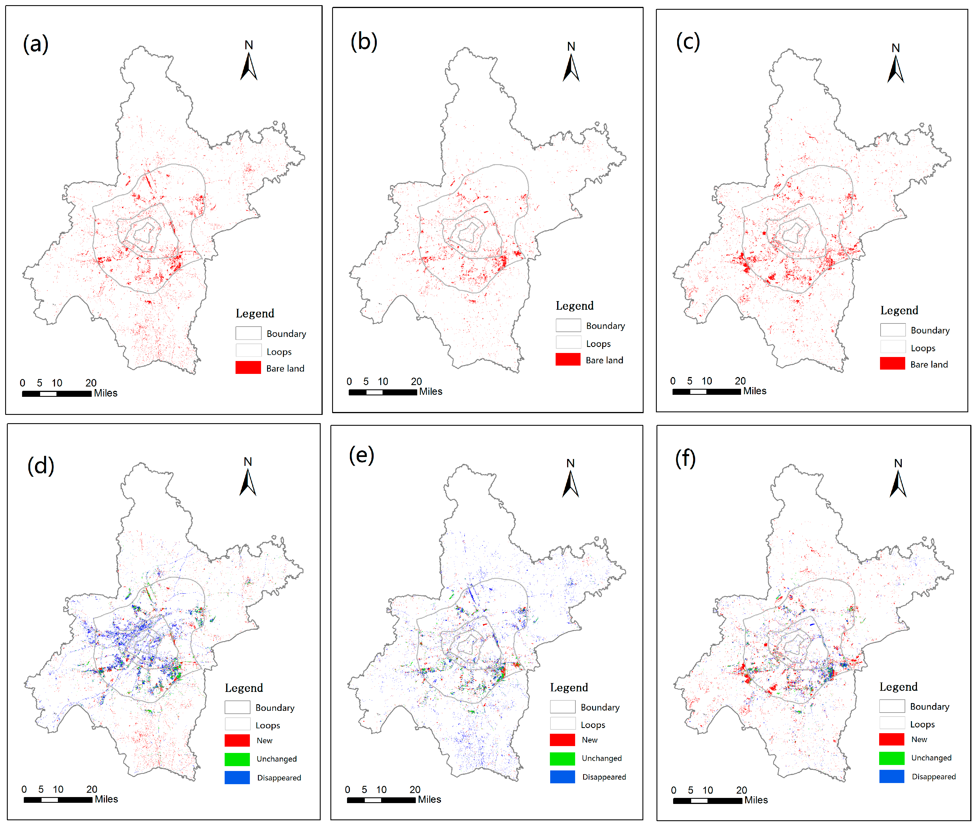
Since 2007, the Wuhan city has been under-going dramatic development and urban expansion. For analyzing the spatial-temporal change of the bare land, the maps of bare land in 2009, 2011, and 2013 were also produced with NBLI. Results are shown in Figure 8,

Table 3. The distribution of bare lands (km²).

	1st Loop *	2nd Loop	3rd Loop	Outer Loop	New *	All *
2007	5.603	22.419	53.136	147.861	——	311.613
2009	1.226	5.965	20.732	109.363	149.596	239.171
2011	0.978	4.729	15.722	86.235	90.161	153.910
2013	0.721	6.008	16.631	117.438	207.707	261.420

* 1st loop is the inner loop. In the table, the 2nd loop means the region between the 1st loop and the 2nd loop, and so on. The column “New” means bare lands appear in this year, and the column “All” includes the new and unchanged.

, and the related accuracy assessment is shown in

Table 4. Accuracy assessment for Wuhan and Shenzhen.

City	Year	Overall Acc. (%)	Kappa Coefficient	Prod. Acc. (%)		User Acc. (%)		Comparison with Reference
				Bare	Other	Bare	Other	Area Ratio	Match Rate (%)
Wuhan	2007	92.00	84.00	84.20	99.80	99.76	86.33	1.13	83.96
	2009	91.25	82.50	85.00	97.50	97.14	86.67	1.21	83.77
	2011	94.00	86.50	87.00	99.50	99.42	88.44	1.15	83.49
	2013	92.25	84.50	86.50	98.00	97.74	87.89	1.12	84.34
Shenzhen	2009	93.00	94.50	86.00	99.90	99.87	87.23	1.10	84.12

.

Figure 8 illustrates that more and more bare lands have appeared around the outer loop, while few bare lands has presented within the inner loops since 2007. From another point of view, most bare lands within inner loops have disappeared, while large bare lands around the outer loop have been booming. In the southwest, the main development is the national Wuhan Economic Development Zone dominated with vehicle production industry. In the east, the main development is the national East Lake High Tech Development Zone, known as the “China’s optic valley”. The two zones are engines to the city’s development.

It is noticed that many bare lands have lasted more than two years. Statistically, 123.0 km² bare lands have existed over two years, 41.6 km² over four years, and 14.7 km² over six years. Authorities should pay attention on how to promote the development of these lands, because the long existence of bare lands may lead to waste of land resource and serious environmental issues.

Table 3 shows that bare lands within the 3rd loop keep decreasing since 2007, implying that lands available for new development become less and less in this region. On the contrary, areas of bare lands around the outer loop have remained high in those years.

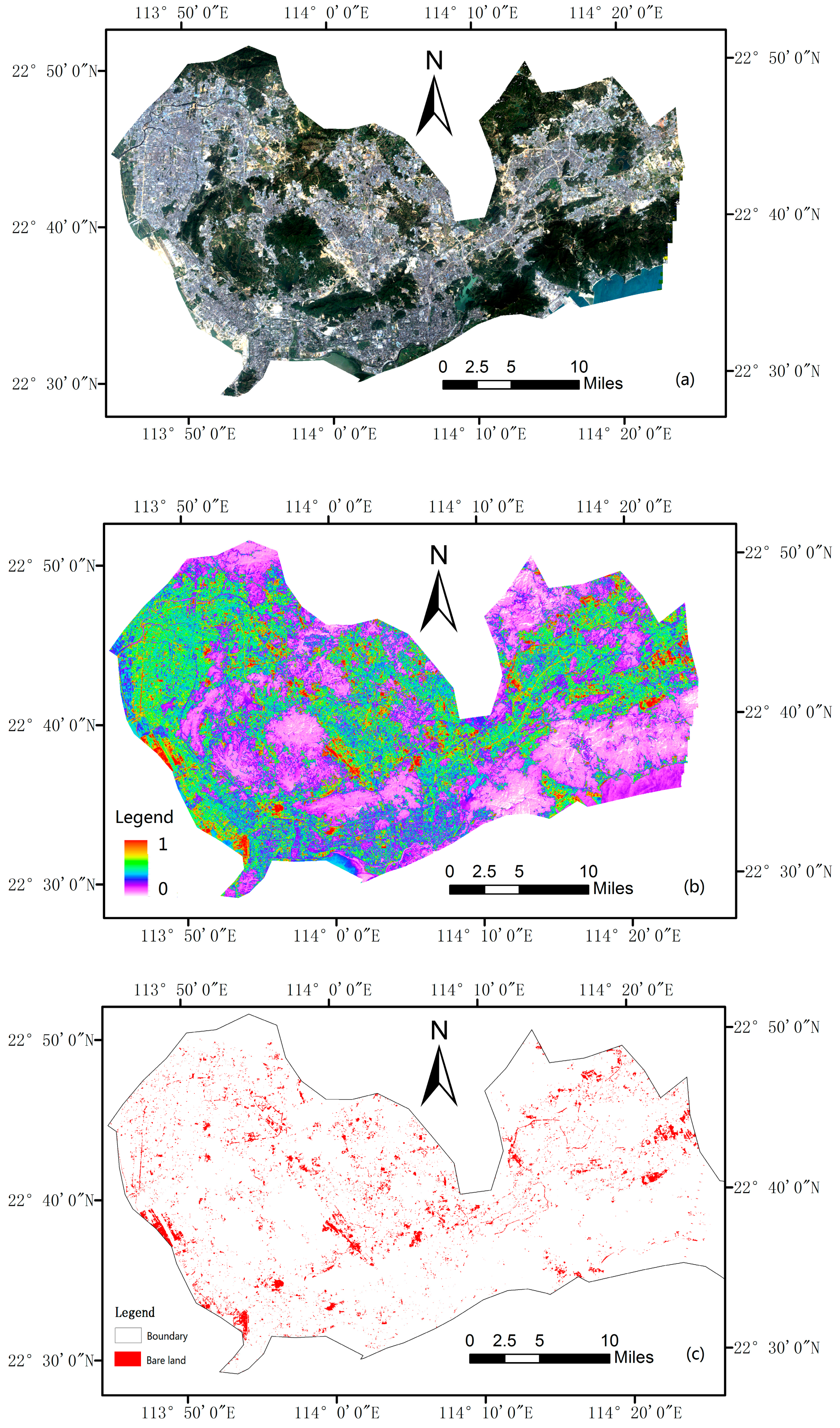
4.4. Another Example: The Shenzhen City

Shenzhen is a major financial center in southern China, located immediately north of Hong Kong. Shenzhen was promoted to a city in 1979 and then the China’s first Special Economic Zone (SEZ) in 1980. Since then, Shenzhen was one of the fastest-growing cities in the world. The city is home to the Shenzhen Stock Exchange, as well as the headquarters of numerous high-tech companies. Shenzhen ranks 19th in the 2016 edition of the Global Financial Centers Index published by the Z/Yen Group and Qatar Financial Centre Authority.

Shenzhen is located within the Pearl River Delta, having a warm, monsoon-influenced, humid subtropical climate. The main land covers in the city includes built up, forest, water and bare land. The proposed method is implemented with Landsat image on 22 November 2009. Results are shown in Figure 9 and Table 4.

Figure 9 shows the proposed method could be successfully implemented in a different region. As there is few agriculture lands and rivers in the city, the differences between the bare land, built up areas and forest are very clear in the index image. In the final result, it is found there is few great bare lands within the city. It illustrates the city is almost developed, although it is very young (since 1979). Oppositely, Wuhan is under great constructions, although its history is very long (since A.D. 233).

5. Discussion

5.1. Characteristics of the Proposed Method

This study proposed a strategy to map the bare land automatically from Landsat imagery with a simple index. First, a novel index NBLI was presented, which could enhance the difference between the bare land and other classes dramatically. Then, an unsupervised classifier was employed to extract the bare land from the NBLI image without training samples. Experiments showed satisfactory mapping results. The NBLI was found to be superior to other urban-related indices by greatly enlarging the difference between the bare land and other classes based on their unique spectral characteristics. This was the trigger to test if it was possible to assign the threshold automatically for bare land extraction. This study demonstrated that the proposed method could effectively produce accurate maps with automatic threshold section.

Several issues about NBLI should be addressed for further applications. First of all, NBLI is sensitive to clouds and aerosols, so atmospheric correction should be performed before calculating the index. Secondly, the quantitative relationship between NBLI and percentage of soil cover is not clear. Thirdly, the index is proven useful when dealing with Landsat images in this study. More tests on other image sources are needed. Last and most importantly, fallow croplands could also be detected as bare lands, as they have similar characteristics as bare land. Actually, it is very difficult to judge if a bare land is a fallow agriculture field or construction site. When focusing on urban bare lands, it is suggested to collect images in the grow seasons, and to analyze those locating within the metropolis circle of a city, where few fallow agricultural fields exist.

5.2. Potential Applications of the Proposed Method

This study points out a potential approach to mapping typical land covers automatically without training samples and self-assigned thresholds. It consists of two main steps: (1) finding an index which is able to highlight the specified land cover very well; and (2) determining the threshold to extract the class automatically. In this study, water bodies within the city have been extracted with the index MNDWI and the k-means classifier. Water removal from the index image significantly improves the accuracy of bare land mapping.

As shown in Figure 4, built-up indices (i.e., IBI, NDBI, and UI) are unable to discriminate the distribution of the built up versus bare land in a clear manner. However, they could highlight both from other lands very well, because the built-up and bare land show similar tendency from the band 4 (NIR) to band 5(SWIR1), which is distinctively different from all of the others. This study shows that the bare land can be extracted accurately with the proposed method. Therefore, the combined application of our NBLI approach and other built-up indices could effectively extract both bare land and urban built-upland, which would provide more accurate outputs in urban mapping.

The most promising application of the proposed strategy would be analyzing times-series satellite images. Mapping the spatial-temporal changes of urban LULC automatically could save considerable cost and time for processing large data sets. This provides great potential for future applications as more and more satellite observations have become available all over the globe.

6. Conclusions

For urban development in a city, the bare land should not be ignored or misclassified because its environmental impacts are often serious. Existing indices are not able to effectively distinguish the bare land from the built up, due to the high degree of land homogeneity and spectral similarity. In this paper, a novel method to map the bare land automatically with Landsat images was presented. A bare soil index NBLI was proposed to dramatically highlight the bare land. Then an unsupervised classifier was employed to extract it automatically. The result showed very good performance based on the overall accuracy, kappa coefficient, area ratio, and match rate. For bare land maps of the study site in multiple years, most bare lands within inner loops disappeared, while large bare lands around outer loops were booming in two main directions. Results illustrate that the proposed method is an accurate and reliable option to map the bare land automatically.

Furthermore, this study points out a promising approach to mapping typical urban LULC automatically with simple indices, which includes: (1) finding an index which is able to highlight the specified types; and (2) classifying the index image with an unsupervised classifier. More experiments and analysis will be implemented in the future to test its feasibility and adoptability in different environments.