A Soil Moisture Retrieval Method Based on Typical Polarization Decomposition Techniques for a Maize Field from Full-Polarization Radarsat-2 Data

Abstract

Soil moisture (SM) estimates are important to research, but are not accurately predictable in areas with tall vegetation. Full-polarization Radarsat-2 C-band data were used to retrieve SM contents using typical polarization decomposition (Freeman–Durden, Yamaguchi and VanZly) at different growth stages of maize. Applicability analyses were conducted, including proportion, regression and surface scattering model analyses. Furthermore, the Bragg, the extended Bragg scattering model (X-Bragg) and improved surface scattering models (ISSM) were used to retrieve SM content. The results indicated that the VanZly decomposition method was the best. The proportion of surface scattering in the proportion analysis was highest (>52%), followed by that in the Yamaguchi method (>41%). The R² (>0.6144) between surface scattering and SM was significantly higher (R² < 0.4484) between dihedral scattering and SM in the regression analysis. The ISSM was better at different maize growth stages than the Bragg and X-Bragg models with a higher R² (>0.6599) and lower absolute error (AE) (<5.82) and root mean square error (RMSE) (<3.73). The best algorithm was obtained at the sowing stage (R² = 0.8843, AE = 3.13, RMSE = 1.76). In addition, the X-Bragg model provided better approximation of actual surface scattering without the measured data (better algorithm: R² = 0.8314, AE = 4.39, RMSE = 2.81).

1. Introduction

Soil moisture (SM) has been one of the most important parameters in the fields of agriculture, the environment and hydrology over the last two decades [1]. In particular, surface SM has been estimated using a series of theoretical, empirical or semi-empirical models according to microwave remote sensing technology [2]. The characteristics of microwave remote sensing provide advantages to detect SM underlying vegetation, such as penetration, multi-polarization and all-time and all-weather observation capability [3,4].

However, most current SM retrieval models are only applicable to bare soil fields based on synthetic aperture radar (SAR) data, such as the integration equation model (IEM), improved IEM and the Oh, Shi, Chen and Dubois electromagnetic models [5,6,7]. In these models, the soil dielectric constant can be regarded as one of the variables. Then, the soil moisture content can be calculated by using Dobson, etc., soil dielectric constant models. Therefore, these electromagnetic models can also be applied to bare soil moisture retrieval models. However, these models are no longer reliable to retrieve SM in areas with vegetation [8]. It is difficult to obtain a signal from the ground using a radar satellite because of the blocking by the vegetation layer [9]. The radar signal not only contains soil information from the ground, but also vegetation information [10]. The most popular SM retrieval model for a field with vegetation is the water cloud model [2], as it only considers two main scattering mechanisms, namely volume scattering from the vegetation and ground scattering from the soil [11]. However, because this model neglects contributions by other scattering sources, it is only applicable to retrieve SM in low-vegetation areas [4].

The multi-polarization characteristics of SAR data must be fully considered to retrieve SM from a field with dense vegetation [12,13]. Polarization decomposition technology is a new method developed in the last two decades [14,15]. However, this technology is mainly used in qualitative research for remote sensing image classification [16], such as quantitative inversion of surface parameters [17,18,19]. The main idea of polarization decomposition technology for quantitative inversion is to divide the scattering matrix into different scattering contributions as the independent contributions are associated with known parameters according to different scattering mechanisms [1,20,21]. The polarization data are decomposed, so data about the influential factors are directly eliminated from the image data to make parameter retrieval possible [22]. Volume scattering data from vegetation are decomposed from ground scattering data to retrieve SM data [1]. Thus, a polarization decomposition method and a component model must be constructed to retrieve SM data from a field with dense vegetation [23].

Methods for polarization decomposition include Freeman–Durden, Yamaguchi, Zhang, An, VanZly, Arii and Wang [24,25]. Depending on the scattering mechanism, the models are grouped as two-component, three-component and four-component decomposition methods [26]. Among them, the most common decomposition method is the three-component method of Freeman–Durden [27]. This method assumes three typical scattering contributions, namely volume scattering from vegetation, surface scattering from the ground and dihedral scattering from the interaction between the ground and the vegetation [28]. The advantages of this method are its simplicity, ease of implementation and quantitative direct elimination of the vegetation effect to retrieve the SM data [29,30,31]. The typical four-component decomposition method is called the Yamaguchi method, which is introduced into the helix scattering component to reduce the proportion of the volume scattering component and increase the proportion of the surface and dihedral scattering components [30]. The VanZly method further corrects the Yamaguchi method, which further reduces volume scattering and increases surface scattering [32]. The maize effect on soil increases gradually as the maize grows [33]. Volume scattering decreases and surface scattering increases to the maximum [34]. In this study, the typical Freeman–Durden, Yamaguchi and VanZly methods were selected to decompose multi-polarization Radarsat-2 data using a covariance matrix.

The surface scattering and dihedral scattering components obtained are directly related to SM content. Dihedral scattering is generally simulated using a dihedral reflector [35]. The most common surface scattering models are the Bragg and X-Bragg models [15,36]. The Bragg model is a simple, small-disturbance model based on Bragg scattering [37]. However, it does not explain the reasons for the power of cross-polarization [37]. It is more suitable for relatively smooth surfaces and long wavebands [28]. The X-Bragg model is improved over the Bragg model on which it is based and solves the problem of the non-zero power of depolarization and cross-polarization [15,36]. However, these models are associated with difficulties in that they are rarely consistent with the actual situation [15]. In this study, the surface scattering model was improved based on data measured at different growth stages of maize and was compared to the Bragg and X-Bragg models.

2. Materials and Methods

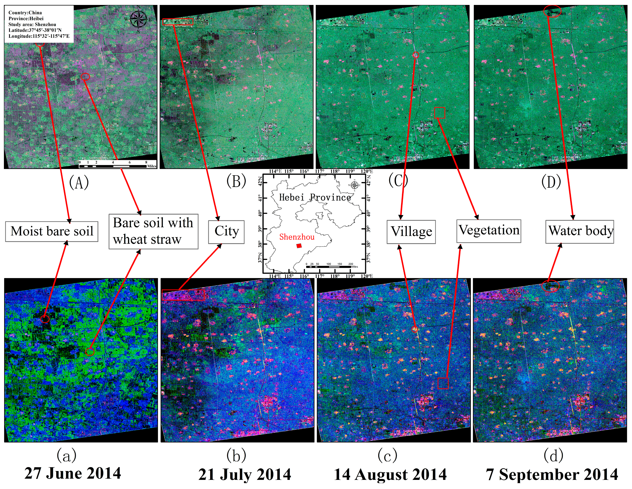
2.1. Study Area and Datasets

2.1.1. Study Area

The study area was located in Hengshui City, Hebei Province, northern China (38°3′00″N, 115°27′54″E) (Figure 1). Field experiments were carried out at a typical agricultural site in Shenzhou. The study area was characterized by homogeneous soil texture, flat terrain and a single crop [38]. Because of this homogeneity, the effects of other factors besides SM were reduced. The main crops in the study area are maize, peanut and cotton in summer [38]. The main soil type is loamy, including about 44.6% silt, 17.5% clay and 37.9% sand [38]. The climate is continental, characterized by high temperature and severe drought in summer. Thus, soil water content is very important for the growth of crops in summer.

The growing period for maize is June–September, and the effect of vegetation on the soil increases as the maize grows. The growing period for maize is divided into sowing, jointing, heading and flowering stages based on morphological and physiological characteristics. No vegetation is present on the land surface at the sowing stage. However, a large amount of wheat straw is left on the land, making the traditional bare SM retrieval models, such as the Oh, Shi and Dubois models, not applicable in this study area. The wheat straw disappears gradually until the jointing stage when the mean leaf area index (LAI) of the maize is about 1.5, the mean leaf age index is approximately 30% and mean plant height is approximately 50 cm. The mean LAI at the heading stage is about 3.0, the mean leaf age index approximately 70% and the mean plant height approximately 200 cm. At the flowering stage, the mean LAI is about 3.5, the mean leaf age index approximately 80% and the mean plant height approximately 250 cm [38].

2.1.2. Imagery and Processing

Radarsat-2 is a high-resolution radar satellite with C-band sensors that was launched by the Canadian Space Agency (Longueuil, QA, Canada) and MDA Corp. (Richmond, BC, Canada) in 2007 [1]. It has four kinds of products and polarization modes. In this study, four polarization single-look complex (SLC) products were selected to retrieve SM [33]. The SLC products retain the optimal resolution and the optimal phase and amplitude information of the SAR data [10]. Four 2014 summer Radarsat-2 scenes were acquired over the Shenzhou study area in the same quad-polarization beam mode (Q19) with 8-m resolution, incidence angles of 38.34–39.82° and an area of 25 × 25 km (

Table 1. RADARSAT-2 image information.

Date	Time UTM	Scene Centre (Lat/Long)	Beam Model	Groundcover Type Number	Dominant Objects
27 June 2014	10:17:30	37.9°N/115.6°E	Q19	6	Bare soil/grasses/orchard
21 July 2014	10:17:30	37.9°N/115.6°E	Q19	5	Bare soil/maize area/orchard
14 August 2014	10:17:30	37.9°N/115.6°E	Q19	4	Maize area/orchard
7 September 2014	10:17:30	37.9°N/115.6°E	Q19	4	Maize area/orchard

Note: the latitude (Lat); the longitude (Long).

) [9].

The Radarsat-2 data were preprocessed using ENVI5.1 and the NEXT ESA SAR Toolbox, including filtering, multi-looking, radiometric correction and geocoding [23]. Multi-looking and filtering were used to increase radiometric resolution and reduce noise. Then, radiometric correction and geocoding were achieved using the Radarsat-2 satellite orbit parameters [20]. Finally, the Radarsat-2 color composite images (RGB) were developed using ENVI5.1 (Figure 1). On the other hand, Radarsat-2 decompositions were calculated using POLSARPRO, ENVI5.1 and ARCGIS10.2. The SLC images were inputted into POLSARPRO software to obtain the images after decomposition. Refined Lee filtering was used to reduce speckle noise [39]. The Freeman–Durden, Yamaguchi and VanZly decomposition methods were carried out in POLSARPRO to obtain different scattering contribution products (dihedral, surface, vegetation volume) [40]. Then, these products were inputted into ENVI5.1 and ARCGIS to define georeferencing using the WGS-1984 projection.

The different colors in the RGB images represent different groundcover types. The imagery shows that the groundcover types are exhibited more clearly in Figure 1a–d than in Figure 1A–D. The image from 27 June 2014 (Figure 1(A,a)) exhibits most of the groundcover types, including moist bare soil, bare soil with wheat straw, the city, the village, the vegetation (grasses and orchards) and water. The bare land (including the moist bare soil and the bare soil area with wheat straw) was covered gradually as the maize grew. The images from 14 August 2014 and 7 September 2014 are similar and exhibit only four groundcover types.

2.1.3. Ground Data

Four field experiments were conducted on the Radarsat-2 satellite overpass dates to ensure the reliability of the ground data (

Table 2. The ground data.

Date	SN	SPN	SMC (g/cm3)	S (cm)	${\mathit{\epsilon }}_{\mathit{r}}$	${\mathit{\rho }}_{\mathbf{soil}}$ (g/cm3)	LAI	EWT (kg/m2)	H (m)	RD (cm)	RS (cm)
27 June 2014	23	64	5.62–48.1	0.4–3.4	2.3–0.1	1.578	0	0	0	0	0
12 July 2014	20	60	6.4–58.4	0.4–5.0	1.3–23.7	1.27	1.37	0.05–2.93	0.57	23.0	40.0
14 August 2014	20	60	9.1–40.9	0.2–3.0	3.7–25.0	1.33	2.89	0.48–5.13	2.19	22.7	41.5
7 September 2014	20	60	8.6–39.3	0.4–2.2	3.4–17.8	1.33	3.35	1.53–3.90	2.58	24.5	41.6

Note: the site number (SN); the sample point number (SPN); the SM volume content (SMC); the root mean square height (S); the soil dielectric constant (${\epsilon }_r$); the mean soil bulk density (${\rho }_{\mathrm{soil}}$); the mean LAI (LAI); the vegetation canopy water content (EWT); the mean maize height (H); the mean ridge distance (RD); the mean row spacing (RS).

). The field campaign measurements were conducted over the bare soil area and maize fields to obtain the soil parameters (moisture, roughness and dielectric constant) and maize parameters (LAI, canopy water content, height, ridge distance and row spacing). A total of 23 typical sample sites were selected in the study area according to the coverage of the Radarsat-2 data (Figure 2). Each sample point was measured three times to eliminate accidental error. Sixty-nine sample points were acquired to develop the SM retrieval algorithms and validate the accuracy of the algorithms. The mean value of three groups was used as the sample point value.

Owing to the weak penetration ability of the C-band, the radar signal only has strong sensitivity to surface SM. Therefore, soil samples were collected at a depth of 0–5 cm to measure SM content using a standard 200-cm cutting ring. The soil samples were sealed in an aluminum box, labeled with a tag and weighed with a balance in near-real time. These soil samples were brought back to the laboratory, dried in a 105 °C drying oven for 24 h and weighed. The soil volume moisture content of each sample was determined according to the weight difference. The dielectric constant of the soil sample was also measured three times using the E5071C Vector Network Analyzer (Keysight Technologies Inc., Santa Rosa, CA, USA) in the laboratory. The mean value was regarded as the point value for each soil sample.

The roughness parameters (root mean square height and correlation length) of the 69 sample points were measured using a needle plate containing 101 pins and a total length of 1 m. Surface roughness was estimated using the mean value of the two directions (east-west and south-north) in the typical position to sample the point at the center. The roughness pictures were corrected to obtain the actual height difference between probes. Then, the coordinates of the vector points for the 101 probes were extracted. The root mean square height and the correlation length were calculated. The roughness of each sample point was measured several times for higher accuracy.

A variety of maize parameters were measured at different growth stages. LAI was measured five times using the LAI-2200C plant canopy analyzer (LI-COR Biosciences, Lincoln, NE, USA). The mean LAI value was regarded as the point value for each soil sample. To determine water content in the maize canopy, fresh maize was collected from each sample plant, weighed and dried in a drying oven. This two-step process was carried out to constant weight, including the 105 °C, 40-min green-killing and the 85 °C, 48-h drying treatments. Furthermore, ridge distance, row spacing and maize height were measured five times with a steel ruler (Table 2).

2.2. Methods

2.2.1. Polarization Decomposition Technique

The scattering signal from vegetation is enhanced gradually as maize grows, leading to weak ground scattering information, which seriously affects the accuracy of SM retrieval. To eliminate this effect, a new method was explored to decompose different scattering contributions directly based on the polarization decomposition technique. The typical polarization decomposition technique is the three-component decomposition model, such as the Freeman–Durden model. The three models used in this study were the Freeman–Durden, Yamaguchi and VanZly models.

The first three-component decomposition method proposed by Freeman and Durden in 1998 decomposes the full-polarization SAR data. This method assumes that the coherency matrix is composed of three typical scattering mechanisms, including surface, volume and double-bounce scattering [28]. Based on the calculated scattering coherency matrix, the Bragg or X-Bragg surface scattering model, the dihedral scattering model and the random direction volume scattering model were applied to this method to separate the scattering information from the vegetation and the soil information from the ground [35].

The coherency matrix is obtained from the Bragg surface scattering model as:

$$\left[T\right]=P_S\left[T_S\right]+P_D\left[T_D\right]+P_V\left[T_V\right]$$

(1)

$$\left[T\right]=f_S\left[\begin{array}{ccc}1& {\beta }^{\ast }& 0\\ \beta & {\left|\beta \right|}^2& 0\\ 0& 0& 0\end{array}\right]+f_D\left[\begin{array}{ccc}{\left|\alpha \right|}^2& \alpha & 0\\ {\alpha }^{\ast }& 1& 0\\ 0& 0& 0\end{array}\right]+\frac{f_V}{4}\left[\begin{array}{ccc}2& 0& 0\\ 0& 1& 0\\ 0& 0& 1\end{array}\right]$$

(2)

$$P=P_S+P_V+P_D=f_S\left(1+{\left|\beta \right|}^2\right)+f_D\left(1+{\left|\alpha \right|}^2\right)+f_V$$

(3)

The coherency matrix is obtained from the X-Bragg surface scattering model as:

$$\left[T\right]=f_S\left[\begin{array}{ccc}1& {\beta }^{\ast }\sin c(2\delta )& 0\\ \beta \sin c(2\delta )& \frac{1}{2}\left|{\beta }^2\right|(1+\sin c(4\delta ))& 0\\ 0& 0& \frac{1}{2}\left|{\beta }^2\right|(1-\sin c(4\delta ))\end{array}\right]+f_D\left[\begin{array}{ccc}\left|{\alpha }^2\right|& \alpha & 0\\ {\alpha }^{\ast }& 1& 0\\ 0& 0& 0\end{array}\right]+f_V\left[\begin{array}{ccc}2& 0& 0\\ 0& 1& 0\\ 0& 0& 1\end{array}\right]$$

(4)

Here, [T] is the total coherency matrix; [T_S], [T_D] and [T_V] are the surface, dihedral and volume scattering component coherency matrix; f_S, f_D and f_V represent the surface, dihedral and volume components of the scattering amplitude, respectively; P, P_S, P_D and P_V represent the total, surface, dihedral and volume components of scattering power; $\beta$ and $\alpha$ represent the surface and dihedral scattering parameters; and $\delta$ represents depolarization.

The Bragg model is a special case of the X-Bragg model. When $\delta$ = 0, the X-Bragg model is the same as the Bragg model [15]. The Bragg model is suitable for relatively smooth surfaces and long wavebands that cannot explain the generation of cross-polarization power. In particular, Freeman et al. (2007) indicated that it is not suitable for bare soil [28]. The X-Bragg model was developed by Hajnsek et al. in 2000 to solve the problem of depolarization and avoid non-zero cross-polarization power [15,35,36]. Furthermore, Hajnsek et al. in 2009 reported that, when $\delta$ = π/6, surface scattering power from the X-Bragg model is maximum and most consistent with the actual ground.

The Yamaguchi method was proposed by Yamaguchi et al. in 2005 and includes four scattering components. The helical scattering component was introduced into polarization decomposition processing, which further increases surface scattering power. Therefore, the Yamaguchi method was an improvement on the Freeman–Durden model [30,31]. In 2005, Yamaguchi et al. thought p($\theta$) (p($\theta$) = sin$\theta$/2) could better reflect the characteristics of tree trunks’ and branches’ azimuthal distribution and was more suitable for the short wave band that was very sensitive to the leaves. Therefore, the Yamaguchi polarization decomposition method can be selected to analyze the maize fields in this study. Among them, the helical scattering model is defined as:

$$\left[T\right]=P_S\left[T_S\right]+P_D\left[T_D\right]+P_V\left[T_V\right]+P_H\left[T_{helix}\right]$$

(5)

$$\left[T_{helix}\right]=\{\begin{array}{c}\left[T_{left\_helix}\right]=\frac{1}{2}\left[\begin{array}{ccc}0& 0& 0\\ 0& 1& j\\ 0& -j& 1\end{array}\right],\mathrm{Im}\left(\left[T_{23}\right]\right)>0\\ \left[T_{right\_helix}\right]=\frac{1}{2}\left[\begin{array}{ccc}0& 0& 0\\ 0& 1& -j\\ 0& j& 1\end{array}\right],\mathrm{Im}\left(\left[T_{23}\right]\right)<0\end{array}$$

(6)

Here, [T_helix] is the helix scattering matrix; [T_{left_helix}] and [T_{right_helix}] are the left and right helix scattering models; Im () is the imaginary part of a complex number; and [T₂₃] is from the coherency matrix.

The existing decomposition methods include model fitting decomposition (MFD) and characteristic value non-negative decomposition (NNED). The Freeman–Durden and Yamaguchi methods are derived from the MFD, and the VanZly was derived from the NNED. In 2011, VanZly et al. indicated that the Freeman–Durden and Yamaguchi methods produce negative eigenvalues, indicating that the volume scattering power was overestimated. The VanZly method was used to subtract the volume scattering component from total scattering to reduce volume scattering power. The residual matrix was decomposed based on the Freeman–Durden method [32]. The residual matrix was:

$$\left[T_{remainder}\right]=\langle \left[T\right]\rangle -P_V\left[T_{Vol}\right]=P_S\left[T_S\right]+P_D\left[T_D\right]+P_X\left[T_X\right]$$

(7)

Here, P_X is the remaining component power and [T_X] is the remaining component in the scattering model and contains partial topography and roughness surface scattering effects.

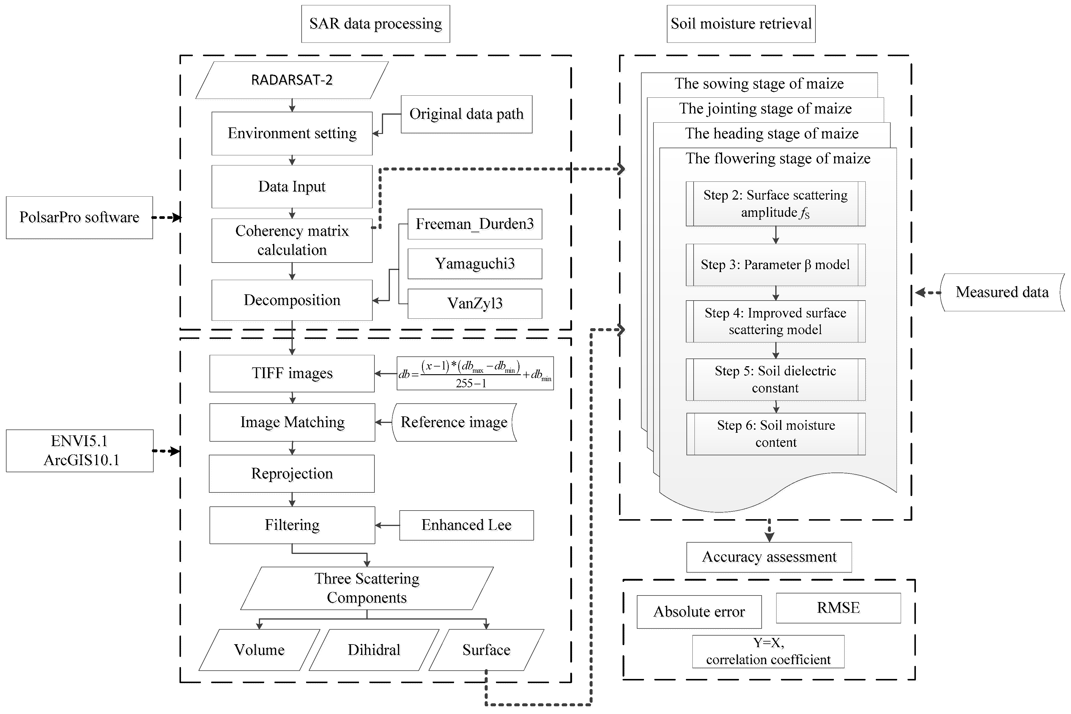
2.2.2. Soil Moisture Content Retrieval Models and Technical Process

The Freeman–Durden, Yamaguchi and VanZly methods are used to calculate surface, volume and double-bounce scattering. Because the surface scattering component is derived from the ground, it excludes the impact from vegetation. Therefore, the SM retrieval models built from the surface scattering component directly eliminate the effect of vegetation on SM. Theoretically, it improves the accuracy of SM retrieval in the vegetation coverage area [15].

In this paper, the typical Bragg and X-Bragg models were used to simulate surface scattering at low frequency [35]. Although the Bragg model is simple, it is only adaptable to a relatively smooth surface area (KS < 0.3). It does not reflect depolarization effects and has a certain gap with actual surface scattering. The X-Bragg model extends the scope of application (KS < 1.0). In this study, the study area is located in the agricultural area of the Northern China Plain. The terrain is simple and flat. The measured surface roughness S ranged from 0.2–5 cm, resulting in the observed roughness as 0.23 < KS < 5.7. When S = 5 cm, this situation is produced only in a few cases. The proportion of measured S ≤ 1 is higher than 80%. Therefore, the X-Bragg and Bragg model were selected and applied to retrieve soil moisture content at the C-band in this study area. However, both the Bragg and X-Bragg models are also not completely consistent with the actual surface scattering. Therefore, the surface scattering models (Bragg and X-Bragg) were improved with measured and theoretical simulation data to obtain more accurate ground scattering information.

P_S, P_D, P_V, $\beta$ and $\alpha$ form Equations (2) and (3). Among them, P_V = 4 × [T₃₃], and P_S, P_D, $\beta$ and $\alpha$ are four unknown parameters. It is assumed that surface scattering is the dominant form of ground scattering to solve $\beta$. In this case, the surface and dihedral scattering components are given by:

$$f_S\left[\begin{array}{ccc}1& {\beta }^{\ast }& 0\\ \beta & {\left|\beta \right|}^2& 0\\ 0& 0& 0\end{array}\right]+f_D\left[\begin{array}{ccc}0& 0& 0\\ 0& 1& 0\\ 0& 0& 0\end{array}\right]=\left[\begin{array}{ccc}S& C& 0\\ C^{\ast }& D& 0\\ 0& 0& 0\end{array}\right]=\left[\begin{array}{ccc}\left[T_{11}\right]-2\left[T_{33}\right]& \left[T_{12}\right]& 0\\ {\left[T_{12}\right]}^{\ast }& \left[T_{22}\right]-\left[T_{33}\right]& 0\\ 0& 0& 0\end{array}\right]$$

(8)

Therefore, surface scattering parameter $\beta$ and amplitude f_S are given by:

$$\beta =\frac{R_h-R_v}{R_h+R_v}, f_s=\frac{S+\raisebox{1ex}{${\left|C\right|}^2$}\!\left/ \!\raisebox{-1ex}{$S$}\right.}{1+{\left|\beta \right|}^2}$$

(9)

$$R_h=\frac{\cos \theta -\sqrt{{\epsilon }_S-{\sin }_{\theta }^2}}{\cos \theta +\sqrt{{\epsilon }_S-{\sin }_{\theta }^2}}, R_v=\frac{\left({\epsilon }_S-1\right)\left({\sin }_{\theta }^2-{\epsilon }_S\left(1+{\sin }_{\theta }^2\right)\right)}{{\left({\epsilon }_S\cos \theta +\sqrt{{\epsilon }_S-}{\sin }_{\theta }^2\right)}^2}$$

(10)

Here, S, C and D are parameters related to the coherency matrix; [T₁₂], [T₂₂] and [T₃₃] are from the coherency matrix; R_h and R_v are the horizontal and vertical Bragg scattering coefficients; ${\epsilon }_S$ is the soil dielectric constant; and $\theta$ is the incidence angle.

The soil dielectric constant was determined from the coherency matrix calculated from the multi-polarized SAR images in Equations (8)–(10). Then, SM content was determined using the dielectric constant model. The measured data (Table 2) were used to correct the Bragg and X-Bragg models and retrieve SM content with higher accuracy. The new models were built with more accuracy, simplification and practicability. The specific steps are as follows:

• Determine the surface scattering component and coherency matrix using POLSARPRO, ENVI5.1 and ARCGIS10.2 from the Radarsat-2 images.
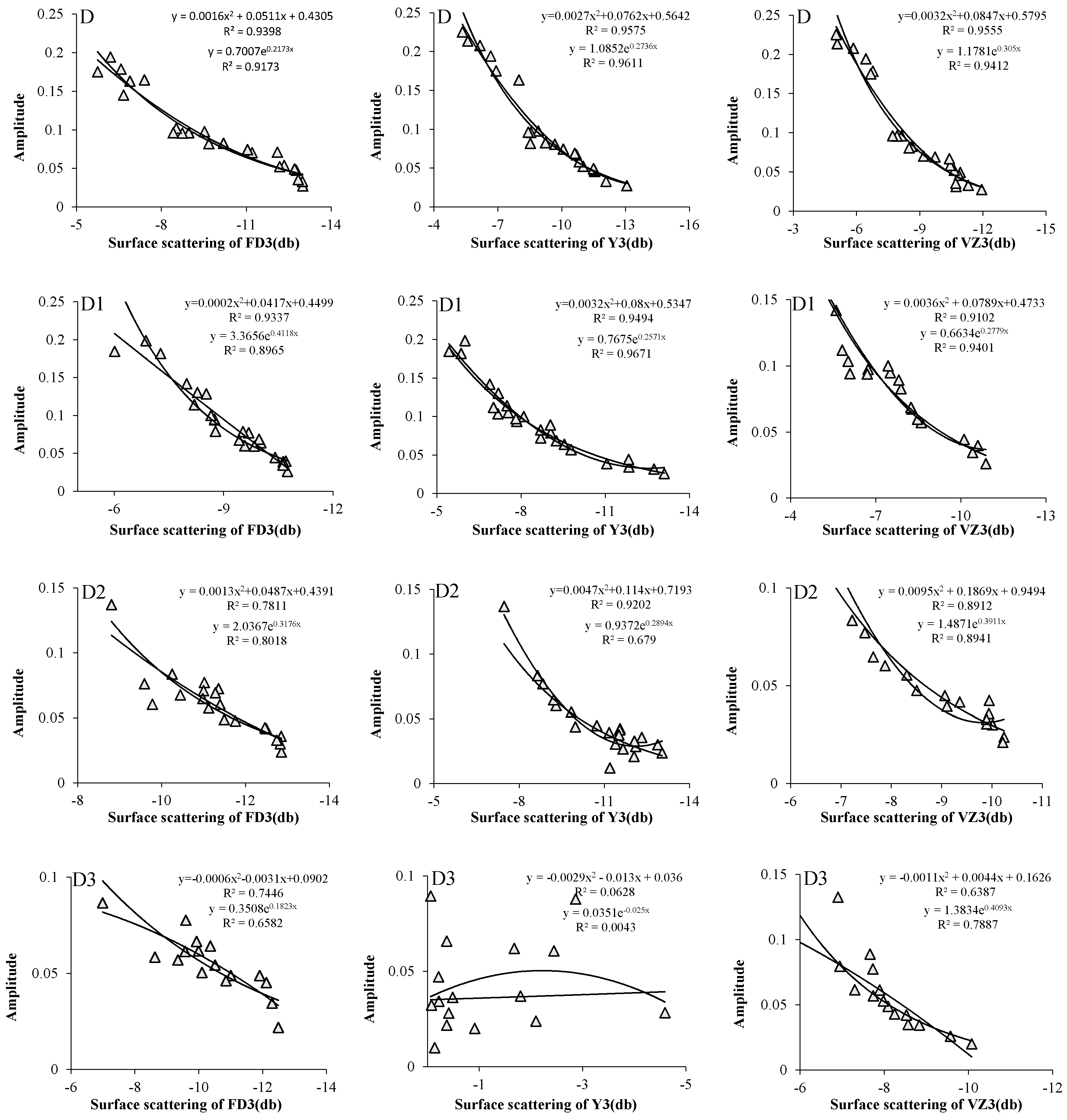
• Build the surface scattering amplitude f_S models from the surface scattering components taken from the different maize growth stages.
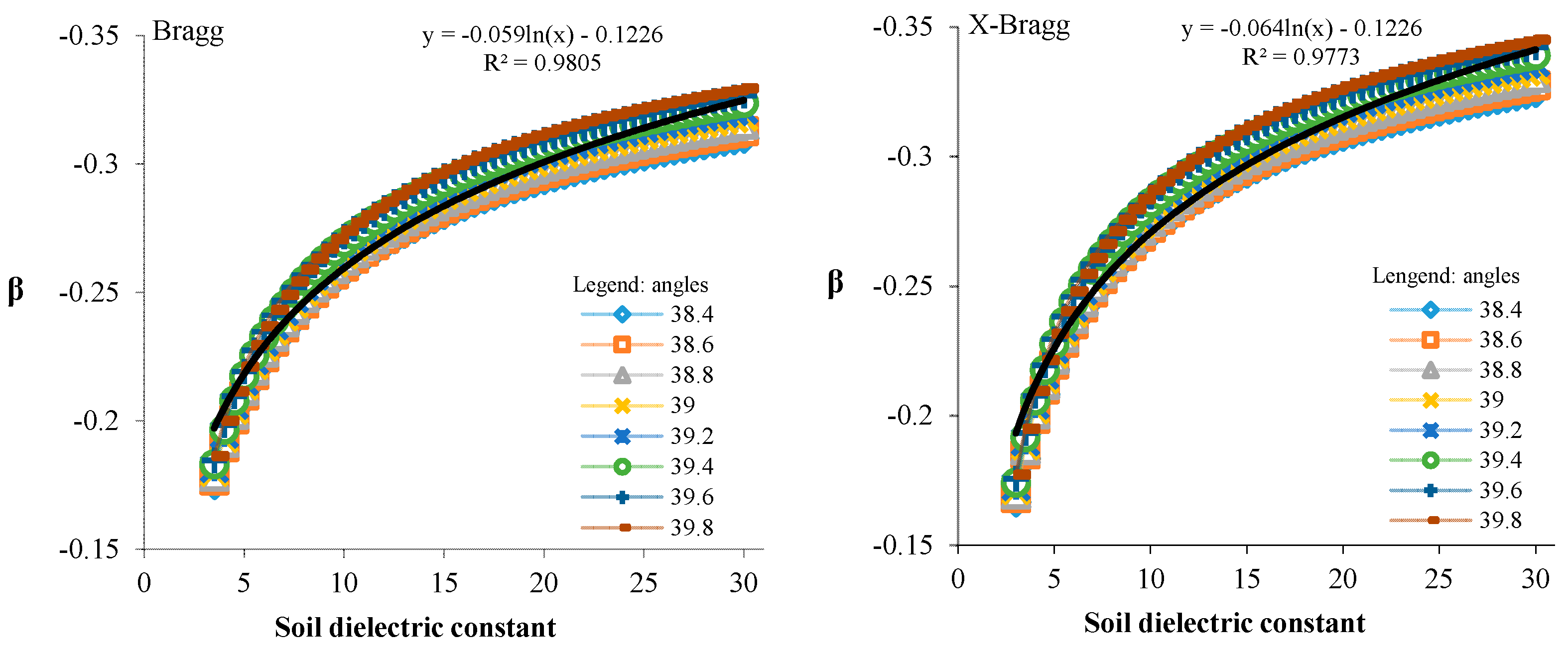
• Calculate the parameter $\beta$ from the f_S model using Equation (9).
• Build the $\beta$ retrieval models based on the measured data and improved Bragg and X-Bragg surface scattering models.
• Calculate the soil dielectric constant from the $\beta$ retrieval model.
• Calculate SM content from the soil dielectric constant model.

In this study, the full-polarization SAR data processing flow was developed to acquire the coherency matrix and the volume, dihedral and surface scattering components. Furthermore, the Bragg and X-Bragg surface scattering models were improved indirectly using the improved parameter $\beta$ models. Then, SM content was retrieved using the soil dielectric constant model. Finally, the levels of accuracy of the different SM retrieval models built based on the three typical polarization decomposition methods were compared and analyzed. The specific technical flow chart is shown in Figure 3.

3. Results

This section shows the results obtained from the analysis of the three typical polarization decomposition methods. To evaluate the limitations and advantages of different polarization decomposition methods, the proportion analysis of the three scattering components was carried out. Then, SM content retrieval regression models and improved surface scattering models were built based on surface and dihedral scattering components.

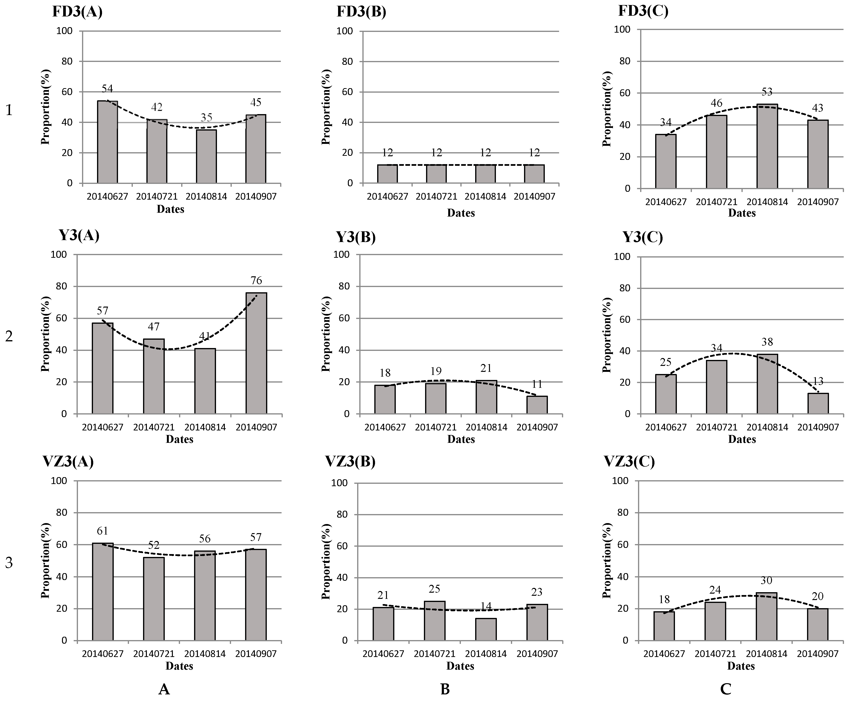
3.1. Proportion Analysis of the Three Scattering Components

The surface scattering component changed constantly as the maize grew. Hajnsek et al. (2009) reported that surface scattering decreases as maize grows. In contrast, volume scattering increases constantly [15]. In addition, there are differences in the scattering component decomposed by different polarization decomposition methods. In this study, it was assumed that surface scattering was the dominant form of ground scattering. Therefore, it was necessary to analyze the changes in the rules of the three scattering components as the maize grew.

In this study, the three scattering components were determined with POLSARPRO software. The proportions of the three scattering components were calculated at the different growth stages of maize (Figure 4).

The dihedral scattering proportion was the lowest (<25%) and had the smallest amplitude change of any maize growth stage (Figure 4(B1,B2,B3). In addition, the dihedral scattering proportion determined using the VanZly method was higher than that using the Yamaguchi or Freeman–Durden method, which were both >14%. The lowest proportion was 11% using the Yamaguchi method on 7 September 2014. The dihedral scattering proportion did not change as the maize grew (Figure 4(B1)). Therefore, the dihedral scattering component was not used to show the SM content. Although it contained some of the soil information, it was not suitable to build the SM retrieval model.

The surface scattering proportion decreased gradually initially and then increased as the maize grew (Figure 4(A1,A2,A3). The opposite was true for the volume scattering (Figure 4(C1,C2,C3). The effect of vegetation on SM is mainly theoretically derived from the vegetation canopy water content. Because the effect of maize on the soil increased gradually from the sowing to the flowering stage, the surface scattering proportion decreased. However, the surface scattering proportion increased suddenly on 7 September 2014, which resulted in a change inconsistent with the regular theoretical change. The reason for this may be that some maize leaves were dry at the flowering stage (Figure 2), which effectively reduces the ground vegetation. This further illustrates that vegetation has a significant impact on SM content. Therefore, the vegetation information must be separated from the radar signal to obtain soil information consistent with the actual ground situation. Surface scattering was the dominant form of ground scattering, and the proportion was >35% to a maximum of 76% (Figure 4(A1,A2,A3). The surface scattering proportion was the highest when using the VanZly method (mean, 56.5%), followed by the Yamaguchi method (mean, 55.25%). The mean proportion of surface scattering determined using the Freeman–Durden method was the lowest (mean, 44%). Thus, the VanZly method could increase the proportion of surface scattering more than the Freeman–Durden and Yamaguchi methods. Form Figure 4(C1,C2,C3), the volume scattering proportion was lower when using the VanZly method (mean, 23%), followed by the Yamaguchi method (mean, 27.5%) and Freeman–Durden method (mean, 44%). The results showed the VanZly method could increase the surface scattering proportion and reduce the volume scattering proportion compared t the Yamaguchi and Freeman–Durden methods.

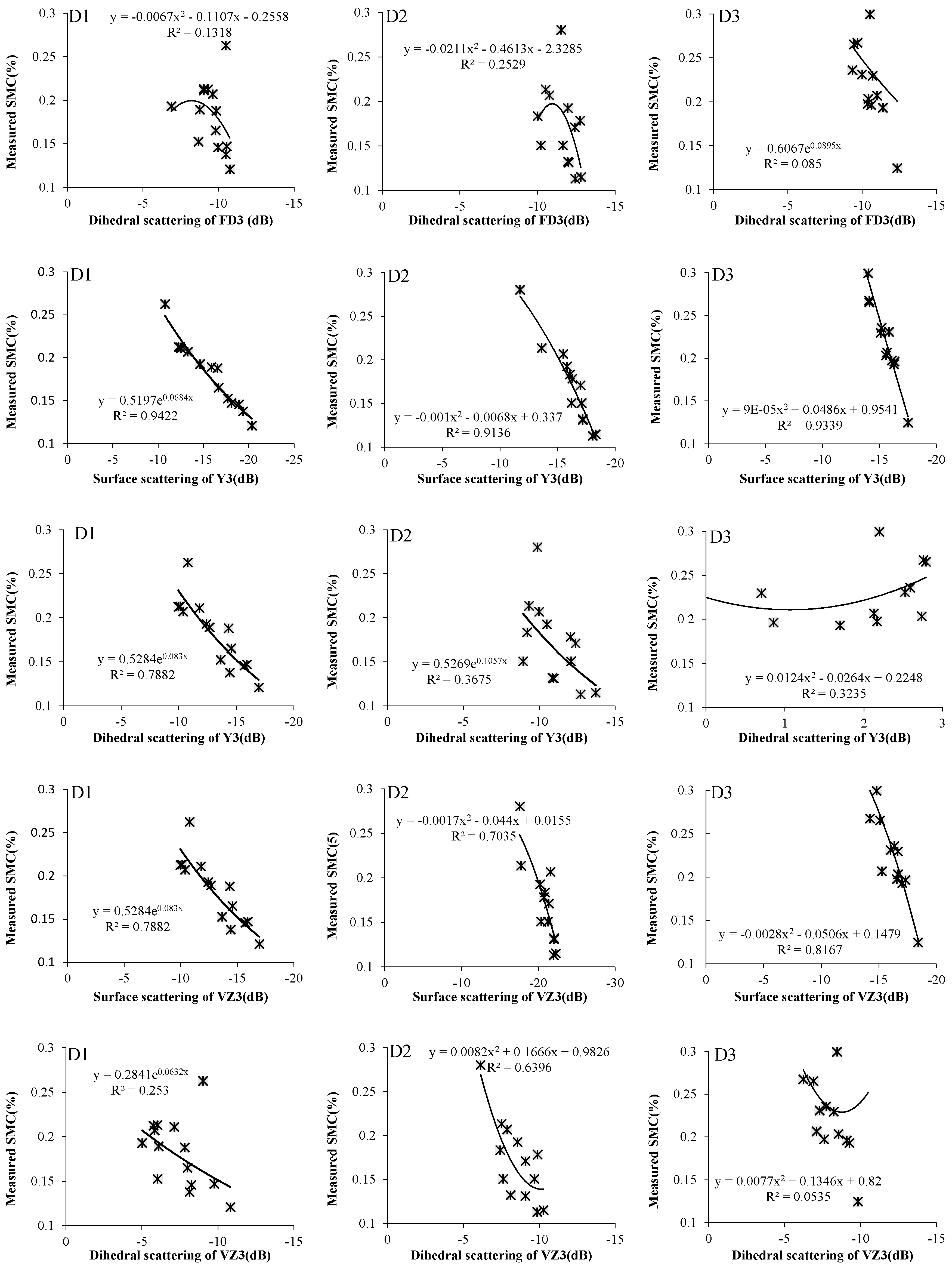
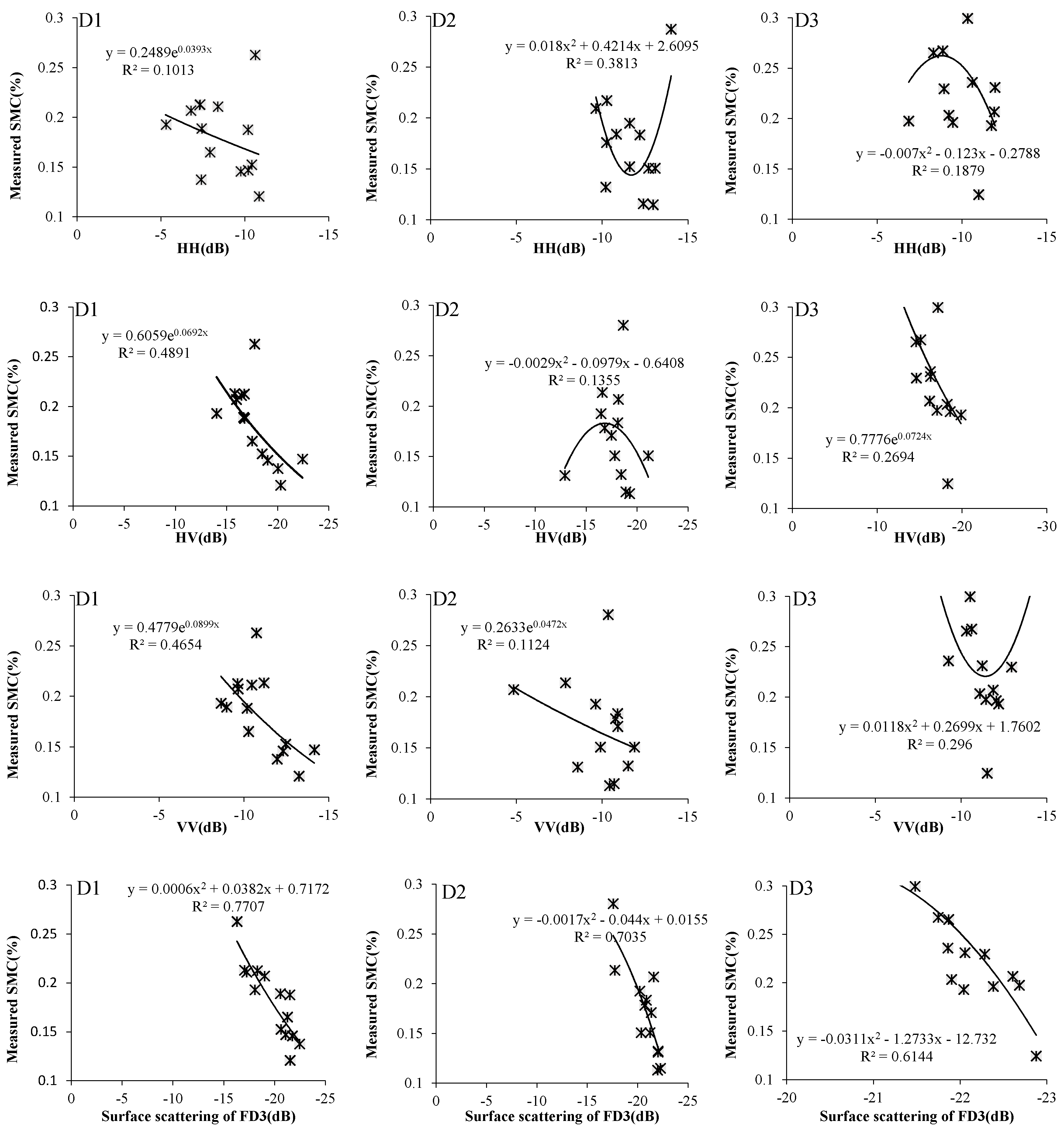
3.2. Regression Models

According to the proportion analyses of the three scattering components, the surface scattering component was the best to retrieve SM content. A regression analysis was performed at different maize growth stages to analyze the relationship between the surface scattering component and SM content (Figure 5). The Radarsat-2 polarization data (HH, HV and VV) and the scattering components (surface and dihedral) were tested to reveal whether they were correlated with SM volume content (SMC). In this study, the linear, polynomial and exponential regression models were selected to analyze the relationship between scattering components and soil moisture content. Finally, the regression models with the highest correlation coefficient were considered as the better regression models at different maize growth stages (Figure 5).

Overall, the correlation coefficient (R² < 0.4484) calculated between HH, HV, the VV Radarsat-2 data and the SMC was significantly lower than that calculated between the scattering components and the measured SMC (R²_max = 0.9384) (Figure 5). The scattering components were more highly correlated with SMC than the original HH, HV and VV data. In this study, it was assumed that when the correlation coefficient of two parameters was less than 0.5, they are just not relevant or their correlations were rather weak. Therefore, the original HH, HV and VV data can be ignored.

In addition, the correlation coefficients (R²_{min_FD3} = 0.6144, R²_{min_Y3} = 0.9136, R²_{min_Y3} = 0.7035) for the relationship between the surface scattering component and the dataset SMC were higher than those for the dihedral scattering component (R²_{max_FD3} = 0.2529, R²_{max_Y3} = 0.7644, R²_{max_Y3} = 0.6396). These results indicate that the surface scattering component is more highly correlated with SMC than the dihedral scattering component. At the same time, the maximum correlation coefficient (R² = 0.9384) was obtained from the Yamaguchi polarization decomposition method (Y3) surface scattering component at the maize jointing stage. The correlation coefficients from the Freeman–Durden polarization decomposition method (FD3) surface scattering component decreased gradually as the maize grew (R²_D1 = 0.7707, R²_D2 = 0.7035, R²_D3 = 0.6144). However, correlation coefficients from the Y3 and VanZly polarization decomposition (VZ3) surface scattering components did not change with growth of the maize (R²_{D1_Y3} = 0.9384, R²_{D2_Y3} = 0.9136, R²_{D3_Y3} = 0.9339, R²_{D1_VZ3} = 0.7644, R²_{D2_VZ3} = 0.7035, R²_{D3_VZ3} = 0.8167), suggesting that the FD3 surface scattering component is strongly affected by vegetation. This finding also shows that the Y3 and VZ3 polarization decomposition methods are better than the FD3. According to this analysis, the scattering components are the most useful to build the SMC retrieval model, particularly the surface scattering component. Second, the Y3 is the best polarization decomposition method for retrieving SMC, followed by VZ3.

3.3. Improved Surface Scattering Model

The regression analysis indicated that the surface scattering component was the most useful to build the SMC retrieval model. The traditional Bragg and X-Bragg surface scattering models were used to decompose the Radarsat-2 polarization data. However, these models are not completely consistent with actual surface scattering [39]. The measured data were used to improve the Bragg and X-Bragg models and obtain more realistic surface scattering. About 20 sample point data were used to establish the empirical relationships. The improved Bragg and X-Bragg models were applied to retrieve SMC. The specific steps are shown in Figure 3.

Different surface scattering models were used at different maize growth stages. The relationship between scattering amplitude and the surface scattering component was determined from the Radarsat-2 images using different polarization decomposition methods (Figure 6).

Surface scattering was strongly associated with amplitude (Figure 6). The correlation was highest on 27 June 2014 (R²_{max_FD3} = 0.9398, R²_{max_Y3} = 0.9611, R²_{max_VZ3} = 0.9555), but tended to decrease as the maize grew. This indirectly suggests that vegetation seriously affects surface scattering. Therefore, although polarization decomposition can theoretically be used to remove the effect of vegetation, it cannot completely eliminate this effect. Y3 was the best polarization decomposition method at the first maize growth stage, followed by FD3 and VZ3 (R²_{FD3_D} = 0.9398, R²_{Y3_D} = 0.9611, R²_{VZ3_D}=0.9555; R²_{FD3_D1} = 0.9337, R²_{Y3_D1} = 9671, R²_{VZ3_D1} = 0.9401; R²_{FD3_D2} = 0.8018, R²_{Y3_D2} = 9202, R²_{VZ3_D2} = 0.8941). However, no correlation was observed between Y3 surface scattering and amplitude at the fourth maize growth stage (R²_{FD3_D3} = 0.7446, R²_{Y3_D3} = 0.0628, R²_{VZ3_D3} = 0.7887). Therefore, Y3 was applicable to the first maize growth stage, and VZ3 was applicable to the fourth growth stage.

Scattering amplitude and $\beta$ parameters were introduced in this study to analyze the relationship between surface scattering and the soil dielectric constant. Scattering amplitude was calculated at different maize growth stages (Figure 6). Then, they were combined with Equation (9) to acquire parameter $\beta$. The soil dielectric constant was determined based on the improved Bragg and X-Bragg ($\delta$ = π/6) models (

Table 3. Surface scattering models at the four growth stages of maize.

Dates	Bragg	XBragg	I-Bragg	IX-Bragg	Improved SSM	N
27 June 2014	y = −0.059ln(x) − 0.1226	y = −0.064ln(x) − 0.1226	y = −0.059ln(Z) − 0.1226 $\mathrm{Z}=e^{\left(0.0474x^2-0.4104x+7.7921\right)}$	y = −0.064ln(Z) − 0.1226 $\mathrm{Z}=e^{\left(0.0437x^2-0.3783x+7.1833\right)}$	y = −0.0028x2 + 0.0242x − 0.5823	20
21 July 2014	y = −0.059ln(x) − 0.1226	y = −0.064ln(x) − 0.1226	y = −0.059ln(Z) − 0.1226 $\mathrm{Z}=e^{\left(0.0859x^2-0.4033x+5.415\right)}$	y = −0.064ln(Z) − 0.1226 $\mathrm{Z}=e^{\left(0.0792x^2-0.3718x+4.9897\right)}$	y = −0.0051x2 + 0.0238x − 0.4419	21
14 August 2014	y = −0.059ln(x) − 0.1226	y = −0.064ln(x) − 0.1226	y = −0.059ln(Z) − 0.1226 $\mathrm{Z}=e^{\left(0.124x^2-1.6442x+12.679\right)}$	y = −0.064ln(Z) − 0.1226 $\mathrm{Z}=e^{\left(0.1143x^2-1.5157x+11.688\right)}$	y = −0.0073x2 + 0.0970x − 0.8707	20
7 September 2014	y = −0.059ln(x) − 0.1226	y = −0.064ln(x) − 0.1226	y = −0.059ln(Z) − 0.1226 $\mathrm{Z}=e^{\left(0.349x^2-5.7503x+29.86\right)}$	y = −0.064ln(Z) − 0.1226 $\mathrm{Z}=e^{\left(0.3217x^2-5.3011x+27.527\right)}$	y = −0.0206x2 + 0.3393x − 1.8843	16

Note: the improved Bragg model (I-Bragg); the improved X-Bragg model (IX-Bragg); the surface scattering model (SSM); the soil dielectric constant parameter (x); the β parameter (y); the intermediate parameter (Z); the number of sample points (N).

). The Bragg and X-Bragg models are only related to the soil dielectric constant and the incidence angle parameters from Equations (10). According to the range of incidence angles on the Radarsat-2 image, the variation in the soil dielectric constant was analyzed with the $\beta$ parameter at the different incidence angles (Figure 7). The change in the soil constant was small at the different incidence angles (Figure 7). Therefore, the Bragg and X-Bragg models can be simplified to logarithmic models. These models well represent the variation in the soil dielectric constant with the $\beta$ parameter (R²_Bragg = 0.9805, R²_X-Bragg = 0.9773).

The Bragg and X-Bragg models were constant throughout the growth of the maize. The simplified Bragg and X-Bragg models were improved using the measured data to acquire more realistic surface scattering at the different growth stages. The improved Bragg (I-Bragg) agreed with the improved X-Bragg model (IX-Bragg) at the same growth stage; therefore, only the improved surface scattering model was determined for the different maize growth stages (Table 3).

3.4. Validation

To validate the applicability of the models (Table 3), each algorithm for the different growth stages was applied to the Radarsat-2 images to retrieve the soil dielectric constant. SM content was calculated using the Dobson soil dielectric constant model. About 15 sample point data were used for the validation in terms of soil moisture retrieval. This model expresses the correlation between the soil dielectric constant and SM content when the frequency is ≥4 GHz [18,41,42,43,44].

The absolute error (AE) and RMSE between the estimated and measured SM were used to assess the surface scattering models at each maize growth stage. The AE reflects the degree of deviation between the estimated and measured SM. The larger the AE, the lower the model precision. The RMSE reflects the overall accuracy of the whole sample and evaluates the advantages and disadvantages of the model as a whole. The accuracy assessment results for the different maize growth stages are shown in

Table 4. Accuracy assessment for all surface scattering models.

Models	AEmax	RMSE	R2	N
ISSM_D	3.13	1.76	0.8843	12
Bragg_D	8.61	3.78	0.4700	12
X-Bragg_D	5.38	2.88	0.6865	12
ISSM_D1	4.48	2.53	0.6874	17
Bragg_D1	5.91	3.16	0.6309	17
X-Bragg_D1	4.91	2.81	0.7288	17
ISSM_D2	3.82	2.28	0.8181	14
Bragg_D2	6.19	2.96	0.5945	14
X-Bragg_D2	5.98	2.82	0.8314	14
ISSM_D3	5.82	3.76	0.6599	17
Bragg_D3	6.82	3.49	0.8301	17
X-Bragg_D3	6.23	3.30	0.8098	17

Note: the maximum absolute error (AEmax); 27 June 2014 (D); 21 July 2014 (D1); 14 August 2014 (D2); 7 September 2014 (D3); the improved surface scattering model (ISSM); the number of sample point (N).

.

The ISSM was the best surface scattering model for the entire growth period. The RMSE was lower in the surface scattering model than in the Bragg and X-Bragg models (mean RMSE, 2.58, 3.42 and 2.95, respectively; Table 4). Thus, the ISSM had good applicability at all maize growth stages. In particular, the RMSE of the ISSM was at a minimum (1.76) on 27 June 2014, and the R² (0.8843) is highest. Surface scattering was not affected by vegetation at the sowing stage. The overall accuracy of the ISSM decreased during growth (RMSE_ISSM__D = 1.76, RMSE_ISSM__D1 = 2.53, RMSE_ISSM__D2 = 2.28, RMSE_ISSM__D3 = 3.76). The accuracy of the ISSM was lower than that for the Bragg and X-Bragg models on 7 September 2014, but the difference was very small. Therefore, the ISSM can also be used to retrieve SM during this period. The accuracy assessment results indicate that the polarization decomposition technique was applicable to reduce the effect of vegetation when retrieving SM content.

On the other hand, the X-Bragg model was clearly better in terms of AE, RMSE or R² at the different growth stages, compared with the conventional Bragg. The Bragg model is too simple, has only two parameters (incidence angle and soil dielectric constant) and is not suitable to retrieve SM in practical applications. In contrast, the X-Bragg model was more consistent with the actual ground. The calculated mean RMSE for the X-Bragg model was 2.95, which is similar to that for the ISSM. Therefore, the X-Bragg model approximated actual surface scattering without measured data.

4. Discussion

At present, polarization decomposition technology is usually used for remote sensing image classification. There are few research works on parameter quantitative retrieval by using polarization decomposition technology [34]. With the development of polarization decomposition technology, it is more and more widely used in parameter quantitative retrieval [1]. Although most research showed that it had a great potential to retrieve soil moisture [34], few research works had been carried out to systematically compare the difference between different polarization decomposition methods [7,39]. Only one was chosen to be used to analyze the relationship between the different scattering component and the volumetric soil moisture content in the study area [45]. In this study, three typical polarization decomposition methods (Freeman–Durden, Yamaguchi and VanZly) were selected to obtain the surface, dihedral and volume scattering components at different maize growth stages [46]. Secondly, proportion and regression analyses of the three scattering components obtained using three typical polarization decomposition techniques were carried out (Figure 4 and Figure 5). The results indicated that the VanZly method was better and could more availably reduce the volume scattering proportion than the Yamaguchi and Freeman–Durden methods (Figure 4). In regression analysis, many studies only emphasized one kind of crop growth stage and polarization decomposition method [47]. At different crop growth stages, there are significant differences in the scattering component decomposed by different polarization decomposition methods [46]. The surface, dihedral and volume scattering components obtained from the same Radarsat-2 data were also obviously different (Figure 4). In this study, the best regression models were built at different maize growth stages based on three polarization decomposition methods (Figure 5).

The conventional surface scattering Bragg and X-Bragg models were used in Freeman-Durden, Yamaguchi, VanZly decomposition, etc. [39,48]. However, because the Radarsat-2 C-band has a shorter wavelength, these models are not completely consistent with actual surface scattering [49]. In this study, according to the incidence angle range of Radarsat-2 data, the change in simulated soil moisture content from the Bragg and X-Bragg was small with incidence angle increasing (Figure 7). Therefore, the Bragg and X-Bragg models were simplified as a logarithmic function (Figure 7). Secondly, the measured soil dielectric constant data were used to improve the Bragg and X-Bragg models (ISSM) at different maize growth stages. The $\beta$ parameter was introduced in this study to analyze the relationship with the soil dielectric constant. Therefore, the ISSM were built at different maize growth stages (Table 3). The best improved surface scattering models were selected according to different maize growth stages (Table 3), which were applied to the inversion of soil moisture content.

The main contributions of this study are as follows: (1) a comparison of three typical polarization decomposition methods (Freeman–Durden, Yamaguchi and VanZly) was carried out by proportion analysis of the three scattering components; VanZly was the best model to availably reduce the volume scattering proportion; (2) the best volumetric soil moisture regression models were built from the surface scattering component at different maize growth stages; (3) according to the measured data, the conventional surface scattering Bragg and X-Bragg models were improved, and the best surface scattering model of different maize growth stages was selected, which basically solved the inconsistent problem with actual surface scattering. Through this study, the research provides new ideas and algorithms for soil moisture retrieval based on the polarization decomposition technique to provide theoretical and technical references.

5. Conclusions

In this study, proportion analyses of the three scattering components obtained using three typical polarization decomposition techniques were carried out to eliminate the effect of vegetation and select the best polarization decomposition method. Then, a regression analysis of the surface and dihedral scattering components was performed to clarify which had the greatest correlation with SM content. Finally, the ISSM was developed based on the Bragg and X-Bragg models at different maize growth stages.

In this study, three typical polarization decomposition methods were used to obtain the surface, dihedral and volume scattering components at different maize growth stages. The results showed that the VanZly method reduced the volume scattering proportion more than that by the Freeman–Durden or Yamaguchi method. Although the dihedral scattering component theoretically contains vegetation and soil information, it did not change during the growth of maize, and the proportion of the component was the smallest. Therefore, the dihedral contribution was inappropriate to retrieve SM as the maize grew. Surprisingly, the correlation between the surface scattering component and SM was significantly higher than that between the dihedral scattering component and SM. The best regression models were selected to retrieve SM using the surface contribution at different maize growth stages.

The use of the volume and dihedral models to build the soil water retrieval models was ruled out. Furthermore, the conventional Bragg and X-Bragg models were applied and improved for use during the entire maize growth cycle. A comparison of the Bragg and X-Bragg models with the ISSM indicated the applicability and advantages of the ISSM at different maize growth stages (RMSE_ISSM__D = 1.76, RMSE_ISSM__D1 = 2.53, RMSE_ISSM__D2 = 2.28, RMSE_ISSM__D3 = 3.76). It further demonstrated that the X-Bragg model had obvious advantages over the Bragg model during the entire maize growing period. However, the ISSM relies on a large number of measured data. When the recorded field SM data were difficult to collect, the X-Bragg model was considered an approximation of actual surface scattering that could be applied to retrieve SM in a maize field.

Although the SM retrieval research by using polarization decomposition techniques has potential to remove the effect of the vegetation, there are some difficulties to build a common model under different underlying surface conditions. At present, the Bayesian retrievals and machine learning algorithms are considered for retrieving SM with a wide range of surface conditions. Different SM retrieval methods have their own advantages and limitations. The next works will be focused on analyzing the adaptability of soil moisture retrieval models built by using different polarization decomposition methods in other study areas. In the future, research and comparison of the polarization decomposition techniques and Bayesian retrievals model, SM retrieval models, etc., will be implemented.

References

1. Bourgeau-Chavez, L.L.; Leblon, B.; Charbonneau, F.; Buckley, J.R. Evaluation of polarimetric Radarsat-2 SAR data for development of soil moisture retrieval algorithms over a chronosequence of black spruce boreal forests. Remote Sens. Environ. 2013, 132, 71–85. [Google Scholar] [CrossRef]
2. Prakash, R.; Singh, D.; Pathak, N.P. A Fusion approach to retrieve soil moisture with SAR and optical data. IEEE J. Sel. Top. Appl. Earth Obs. Remote Sens. 2012, 5, 196–206. [Google Scholar] [CrossRef]
3. Baghdadi, N.; Holah, N.; Zribi, M. Calibration of the integral equation model for SAR data in C-band and HH and VV polarizations. Int. J. Remote Sens. 2006, 27, 805–816. [Google Scholar] [CrossRef]
4. Joseph, A.T.; Van Der Velde, R.; O’Neill, P.E.; Lang, R.; Gish, T. Effects of corn on C- and L-band radar backscatter: A correction method for soil moisture retrieval. Remote Sens. Environ. 2010, 114, 2417–2430. [Google Scholar] [CrossRef]
5. Oh, Y.; Jung, S.G. Inversion algorithm for soil moisture retrieval from polarimetric ackscattering coefficients of vegetation canopies. In Proceedings of the IEEE International Geoscience and Remote Sensing Symposium, Boston, MA, USA, 7–11 July 2008; pp. II-402–II-405.
6. Park, S.; Kweon, S.K.; Oh, Y. Validity regions of soil moisture retrieval on the mboxLAIθ plane for agricultural fields at L-, C-, and X-bands. IEEE Geosci. Remote Sens. Lett. 2015, 12, 1–4. [Google Scholar]
7. Shi, J.; Lee, J.S.; Chen, K.; Sun, Q. Evaluate usage of decomposition technique in estimation of soil moisture with vegetated surface by multi-temporal measurements. In Proceedings of the IEEE International Geoscience and Remote Sensing Symposium, Honolulu, HI, USA, 24–28 July 2000; pp. 1098–1100.
8. Zribi, M.; Dechambre, M. A new empirical model to retrieve soil moisture and roughness from C-band radar data. Remote Sens. Environ. 2003, 84, 42–52. [Google Scholar] [CrossRef]
9. Lievens, H.; Verhoest, N.E.C. Spatial and temporal soil moisture estimation from Radarsat-2 imagery over Flevoland, The Netherlands. J. Hydrol. 2012, 456–457, 44–56. [Google Scholar] [CrossRef]
10. Gherboudj, I.; Magagi, R.; Berg, A.A.; Toth, B. Soil moisture retrieval over agricultural fields from multi-polarized and multi-angular RADARSAT-2 SAR data. Remote Sens. Environ. 2011, 115, 33–43. [Google Scholar] [CrossRef]
11. Attema, E.P.W.; Ulaby, F.T. Vegetation model as a water cloud. Radio Sci. 1978, 13, 357–364. [Google Scholar] [CrossRef]
12. Jun, J.; Yang, J. Multi-polarization reconstruction from compact polarimetry based on modified four-component scattering decomposition. J. Syst. Eng. Electr. 2014, 25, 399–410. [Google Scholar]
13. Kang, M.K.; Kim, K.E.; Lee, H.Y.; Cho, S.J.; Lee, J.H. Preliminary results of polarimetric characteristics for C-band quad-polarization GB-SAR images using H/A/polarimetric decomposition theorem. Korean J. Remote Sens. 2009, 25, 531–546. [Google Scholar]
14. Ghosh, N.; Wood, M.F.; Vitkin, I.A. Mueller matrix decomposition for extraction of individual polarization parameters from complex turbid media exhibiting multiple scattering, optical activity, and linear birefringence. J. Biomed. Opt. 2008, 13, 44036. [Google Scholar] [CrossRef] [PubMed]
15. Hajnsek, I.; Cloude, S.R.; Lee, J.S.; Pottier, E. Inversion of surface parameters from polarimetric SAR data. In Proceedings of the IEEE International Geoscience and Remote Sensing Symposium, Honolulu, HI, USA, 24–28 July 2000; pp. 1095–1097.
16. Liu, X.; Xiao, H.; Yue, C.; University, S.F. Research on ground objects types recognition method based on polarization target decomposition. For. Inventory Plan. 2015, 40, 1–4. [Google Scholar]
17. Dong, Y.; Forster, B.; Ticehurst, C. Polarimetric image classification using optimal decomposition of radar polarization signatures. In Proceedings of the International Geoscience and Remote Sensing Symposium, ‘Remote Sensing for a Sustainable Future’, Lincoln, NE, USA, 31 May 1996; pp. 1556–1558.
18. Dobson, M.C.; Ulaby, F.T.; Hallikainen, M.T.; El-Rayes, M.A. Microwave dielectric behavior of wet soil-Part II: Dielectric mixing models. IEEE Trans. Geosci. Remote Sens. 1985, 23, 35–46. [Google Scholar] [CrossRef]
19. Feng, X.; Wang, H.; Jin, Y.Q.; Liu, X.; Wang, R.; Deng, Y. Impact of cross-polarization isolation on polarimetric target decomposition and target detection. Radio Sci. 2015, 50, 327–338. [Google Scholar]
20. Touzi, R.; Deschamps, A.; Rother, G. Wetland characterization using polarimetric Radarsat-2 capability. Can. J. Remote Sens. 2007, 33, S56–S67. [Google Scholar] [CrossRef]
21. Wei, Z.; Jian, L.; Ling, C.; Yang, J.Z. Geological information extraction using polarimetric SAR based on polarization decomposition. Remote Sens. Inf. 2014, 29, 10–14. [Google Scholar]
22. Li, Y.; Zhao, K.; Zheng, X.; Ren, J.; Ding, Y.; Wu, L. Identification of saline-alkali soil based on target decomposition of full-polarization radar data. J. Appl. Remote Sens. 2014, 8, 1095–1096. [Google Scholar] [CrossRef]
23. Pasolli, L.; Notarnicola, C.; Bruzzone, L.; Bertoldi, G.; Chiesa, S.D.; Niedrist, G.; Tappeiner, U.; Zebisch, M. Polarimetric Radarsat-2 imagery for soil moisture retrieval in alpine areas. Can. J. Remote Sens. 2012, 37, 535–547. [Google Scholar] [CrossRef]
24. Wang, Y.; Ainsworth, T.L.; Lee, J.S. Assessment of system polarization quality for polarimetric SAR imagery and target decomposition. IEEE Trans. Geosci. Remote Sens. 2011, 49, 1755–1771. [Google Scholar] [CrossRef]
25. Wang, H.; Huang, Q.; Pi, Y. Polarization decomposition with S and T matrix of a PolSAR image. In Proceedings of the International Conference on IEEE Communications, Circuits and Systems, Milpitas, CA, USA, 23–25 July 2009.
26. Zhang, C.Z.; Zhang, J.; Liu, C.Y.; Li, L. Polarization decomposition algorithm for detection efficiency enhancement. Radioengineering 2013, 22, 1041–1047. [Google Scholar]
27. Deng, L.; Yan, Y. Improving the Yamaguchi4 decomposition method using selective polarization orientation compensation. Can. J. Remote Sens. 2016, 42, 125–135. [Google Scholar] [CrossRef]
28. Freeman, A. Fitting a two-component scattering model to polarimetric SAR data from forests. IEEE Trans. Geosci. Remote Sens. 2007, 45, 2583–2592. [Google Scholar] [CrossRef]
29. Wang, H.; Magagi, R.; Goita, K.; Jagdhuber, T. Evaluation of polarimetric decomposition for soil moisture retrieval over vegetated agricultural fields. In Proceedings of the IEEE International Geoscience and Remote Sensing Symposium, Milan, Italy, 26–31 July 2015; pp. 689–692.
30. Yamaguchi, Y.; Yajima, Y.; Yamada, H. A four-component decomposition of POLSAR images based on the coherency matrix. IEEE Geosci. Remote Sens. Lett. 2006, 3, 292–296. [Google Scholar] [CrossRef]
31. Yamaguchi, Y.; Moriyama, T.; Ishido, M.; Yamada, H. Four-component scattering model for polarimetric sar image decomposition. IEEE Trans. Geosci. Remote Sens. 2005, 43, 1699–1706. [Google Scholar] [CrossRef]
32. Zyl, J.J.V.; Arii, M.; Kim, Y. Model-based decomposition of polarimetric SAR covariance matrices constrained for nonnegative eigenvalues. IEEE Trans. Geosci. Remote Sens. 2011, 49, 3452–3459. [Google Scholar]
33. Charbonneau, F. Using RADARSAT-2 polarimetric and ENVISAT-ASAR dual-polarization data for estimating soil moisture over agricultural fields. Can. J. Remote Sens. 2012, 38, 514–527. [Google Scholar]
34. Jagdhuber, T.; Hajnsek, I.; Bronstert, A. Soil moisture estimation under low vegetation cover using a multi-angular polarimetric decomposition. IEEE Trans. Geosci. Remote Sens. 2013, 51, 2201–2215. [Google Scholar] [CrossRef]
35. Lee, J.S.; Ainsworth, T.L. The effect of orientation angle compensation on coherency matrix and polarimetric target decompositions. IEEE Trans. Geosci. Remote Sens. 2011, 49, 53–64. [Google Scholar] [CrossRef]
36. Hajnsek, I.; Jagdhuber, T.; Schon, H.; Papathanassiou, K.P. Potential of estimating soil moisture under vegetation cover by means of polsar. IEEE Trans. Geosci. Remote Sens. 2009, 47, 442–454. [Google Scholar] [CrossRef]
37. Ossikovski, R. Integral decomposition and polarization properties of depolarizing Mueller matrices. Opt. Lett. 2015, 40, 954–957. [Google Scholar] [CrossRef] [PubMed]
38. Meng, Q.Y.; Xie, Q.X.; Wang, C.M.; Ma, J.X.; Sun, Y.X.; Zhang, L.L. A fusion approach of the improved Dubois model and best canopy water retrieval models to retrieve soil moisture through all maize growth stages from Radarsat-2 and Landsat-8 data. Environ. Earth Sci. 2016, 75, 1377. [Google Scholar] [CrossRef]
39. Huang, X.; Wang, J.; Shang, J. An adaptive two-component model-based decomposition on soil moisture estimation for C-band Radarsat-2 imagery over wheat fields at early growing stages. IEEE Geosci. Remote Sens. Lett. 2016, 13, 414–418. [Google Scholar] [CrossRef]
40. Huang, X.; Wang, J.; Shang, J. An integrated surface parameter inversion scheme over agricultural fields at early growing stages by means of C-band polarimetric Radarsat-2 imagery. IEEE Trans. Geosci. Remote Sens. 2016, 54, 2510–2528. [Google Scholar] [CrossRef]
41. Gharechelou, S.; Tateishi, R.; Sumantyo, J.T.S. Interrelationship analysis of L-band backscattering intensity and soil dielectric constant for soil moisture retrieval using PALSAR data. Adv. Remote Sens. 2015, 4, 1–10. [Google Scholar] [CrossRef]
42. Hallikainen, M.T.; Ulaby, F.T.; Dobson, M.C.; Elrayes, M.A.; Wu, L. Microwave dielectric behavior of wet soil-part 1: Empirical models and experimental observations. IEEE Trans. Geosci. Remote Sens. 1985, 23, 25–34. [Google Scholar] [CrossRef]
43. Mialon, A.; Richaume, P.; Leroux, D.; Bircher, S.; Al Bitar, A.; Pellarin, T.; Wigneron, J.P.; Kerr, Y.H. Comparison of Dobson and Mironov dielectric models in the SMOS soil moisture retrieval algorithm. IEEE Trans. Geosci. Remote Sens. 2015, 53, 3084–3094. [Google Scholar] [CrossRef]
44. Topp, G.C.; Davis, J.L.; Annan, A.P. Electromagnetic determination of soil water content: Measurements in coaxial transmission lines. Water Resour. Res. 1980, 16, 574–582. [Google Scholar] [CrossRef]
45. Di Martino, G.; Iodice, A.; Natale, A.; Riccio, D. Polarimetric two-scale two-component model for the retrieval of soil moisture under moderate vegetation via L-band SAR data. IEEE Trans. Geosci. Remote Sens. 2016, 54, 2470–2491. [Google Scholar] [CrossRef]
46. He, L.; Panciera, R.; Tanase, M.A.; Walker, J.P.; Qin, Q. Soil moisture retrieval in agricultural fields using adaptive model-based polarimetric decomposition of SAR data. IEEE Trans. Geosci. Remote Sens. 2016, 54, 4445–4460. [Google Scholar] [CrossRef]
47. Wang, P.; Zhou, Z.; Liao, J. Study on soil moisture retrieval of tobacco field in karst plateau mountainous area based on freeman decomposition. Geogr. Geo-Inf. Sci. 2016, 32, 72–76. [Google Scholar]
48. Ponnurangam, G.G.; Jagdhuber, T.; Hajnsek, I.; Rao, Y.S. Soil moisture estimation using hybrid polarimetric SAR Data of RISAT-1. IEEE Trans. Geosci. Remote Sens. 2016, 54, 2033–2049. [Google Scholar] [CrossRef]
49. Wang, H.; Magagi, R.; Goita, K.; Jagdhuber, T.; Hajnsek, I. Evaluation of simplified polarimetric decomposition for soil moisture retrieval over vegetated agricultural fields. Remote Sens. 2016, 8, 142. [Google Scholar] [CrossRef]
Figure 1. Location of the study area and RGB images ((AD) R: HH polarization data; G: HV polarization data; B: VV polarization data) ((ad) R: dihedral scattering product; G: volume scattering product; B: surface scattering product).
Remotesensing 09 00168 g001
Figure 2. Experimental path, sampling strategy and representative field photos.
Remotesensing 09 00168 g002
Figure 3. Flow chart of the Radarsat-2 data processing and soil moisture (SM) retrieval.
Remotesensing 09 00168 g003
Figure 4. Proportion change distribution of the three scattering components with the growth of maize (FD3: the Freeman–Durden polarization decomposition method; Y3: the Yamaguchi polarization decomposition method; VZ3: the VanZly polarization decomposition; (A) the surface scattering component; (B) the dihedral scattering component; (C) the volume scattering component).
Remotesensing 09 00168 g004
Figure 5. Regression analysis between the HH, HV, VV RADARSAT-2 data, surface scattering component, dihedral scattering component and the measured SM content at the different growth stage of maize (FD3: the Freeman–Durden polarization decomposition method; Y3: the Yamaguchi polarization decomposition method; VZ3: the VanZly polarization decomposition; D1: 21 July 2014; D2: 14 August 2014; D3: 7 September 2014).
Remotesensing 09 00168 g005aRemotesensing 09 00168 g005b
Figure 6. Scattering amplitude models at the different growth stages of maize (FD3: the Freeman–Durden polarization decomposition method; Y3: the Yamaguchi polarization decomposition method; VZ3: the VanZly polarization decomposition; D: 27 June 2014; D1: 21 July 2014; D2: 14 August 2014; D3: 7 September 2014).
Remotesensing 09 00168 g006
Figure 7. The Bragg and X-Bragg models analysis at the different incidence angles from Radarsat-2.
Remotesensing 09 00168 g007