Salt Marsh Monitoring in Jamaica Bay, New York from 2003 to 2013: A Decade of Change from Restoration to Hurricane Sandy

Abstract

This study used Quickbird-2 and Worldview-2, high resolution satellite imagery, in a multi-temporal salt marsh mapping and change analysis of Jamaica Bay, New York. An object-based image analysis methodology was employed. The study seeks to understand both natural and anthropogenic changes caused by Hurricane Sandy and salt marsh restoration, respectively. The objectives of this study were to: (1) document salt marsh change in Jamaica Bay from 2003 to 2013; (2) determine the impact of Hurricane Sandy on salt marshes within Jamaica Bay; (3) evaluate this long term monitoring methodology; and (4) evaluate the use of multiple sensor derived classifications to conduct change analysis. The study determined changes from 2003 to 2008, 2008 to 2012 and 2012 to 2013 to better understand the impact of restoration and natural disturbances. The study found that 21 ha of salt marsh vegetation was lost from 2003 to 2013. From 2012 to 2013, restoration efforts resulted in an increase of 10.6 ha of salt marsh. Hurricane Sandy breached West Pond, a freshwater environment, causing 3.1 ha of freshwater wetland loss. The natural salt marsh showed a decreasing trend in loss. Larger salt marshes in 2012 tended to add vegetation in 2012–2013 (F₄,₆ = 13.93, p = 0.0357 and R² = 0.90). The study provides important information for the resource management of Jamaica Bay.

1. Introduction

Jamaica Bay, an estuary within the New York City (NYC) limits, is heavily influenced by urbanization. The salt marshes serve as an interface between the Bay and surrounding urban areas. Currently, over a dozen marsh islands span the Bay. Their landscapes are composed of mudflats, a variety of salt marsh plant species, sediment deposited to rebuild drowning salt marsh, transitional vegetation denoting the shift to upland, and human created upland areas. Salt marshes provide numerous ecological benefits such as high biodiversity, improved water quality, flood reduction, and carbon sequestration [1]. The wetland ecosystems of New York State, including salt marshes, were reduced by 60% from 1780 to 1980 [2]. Nationally, salt marshes have been under particular stress with increasing rates of loss from 2004 to 2009 caused in part by coastal storms [3]. In the past, these trends were exacerbated in the urban-impacted Jamaica Bay.

Jamaica Bay’s salt marsh loss is severe. Since 1951, approximately 60% of the Bay’s salt marsh has converted into mudflats due to a combination of factors including a reduction in sediment supply, changes in tidal regime, nutrient enrichment and increased hydrogen sulfide concentrations [4]. This estimate does not include areas of wetlands around the estuary lost to land filling and urbanization. From 1989 to 2003, Jamaica Bay’s salt marshes were in rapid decline losing 13.4 ha/year [5]. The nitrogen load of the Bay is one factor that may contribute to this high rate of loss [6].

Remote sensing is uniquely suited for monitoring coastal environments, due to the difficulty of in situ access and the high temporal resolution required to understand these dynamic landscapes [7]. Remote sensing monitoring of the salt marsh landscape can be used to determine vegetation trends for the entire bay and individual islands, facilitating an assessment of restoration impacts. Remote sensing is an important tool for furthering our understanding of how Jamaica Bay’s salt marshes are affected by anthropogenic and natural factors [8,9]. This study used imagery data spanning a decade and two high resolution sensor systems.

In October 2012, Hurricane Sandy impacted the coast of New York and surrounding states with high winds and storm surge. It was a 500-year storm surge event at the Manhattan Battery [10]. The boroughs of Brooklyn and Queens directly surrounding Jamaica Bay were inundated; the storm caused two million New Yorkers to lose power [11]. This study seeks to understand the impact of Hurricane Sandy on salt marsh vegetation within Jamaica Bay. The salt marsh vegetation types of interest are smooth cordgrass (S. alterniflora), high marsh (a mixture of Distichlis spicata, Spartina patens, and Juncus gerardii) and the common reed (Phragmites australis). Successful management of Jamaica Bay is contingent on continuing to further our understanding of the change experienced by the Bay’s salt marshes due to both natural disturbance and human impacts.

The objectives of this study were to: (1) document salt marsh changes that occurred in Jamaica Bay from 2003 to 2013; (2) determine the impact of Hurricane Sandy on salt marshes within Jamaica Bay; (3) evaluate this long-term monitoring methodology for the determination of change; and (4) evaluate the use of multiple sensor derived classifications to conduct change analysis. The combination of climate change, sea level rise and their impacts on natural disturbances are expected to have detrimental effects on coastal salt marshes [12]; thereby, enhancing the need for accurate remote sensing monitoring and assessment of coastal wetlands to inform decision-makers.

2. Materials and Methods

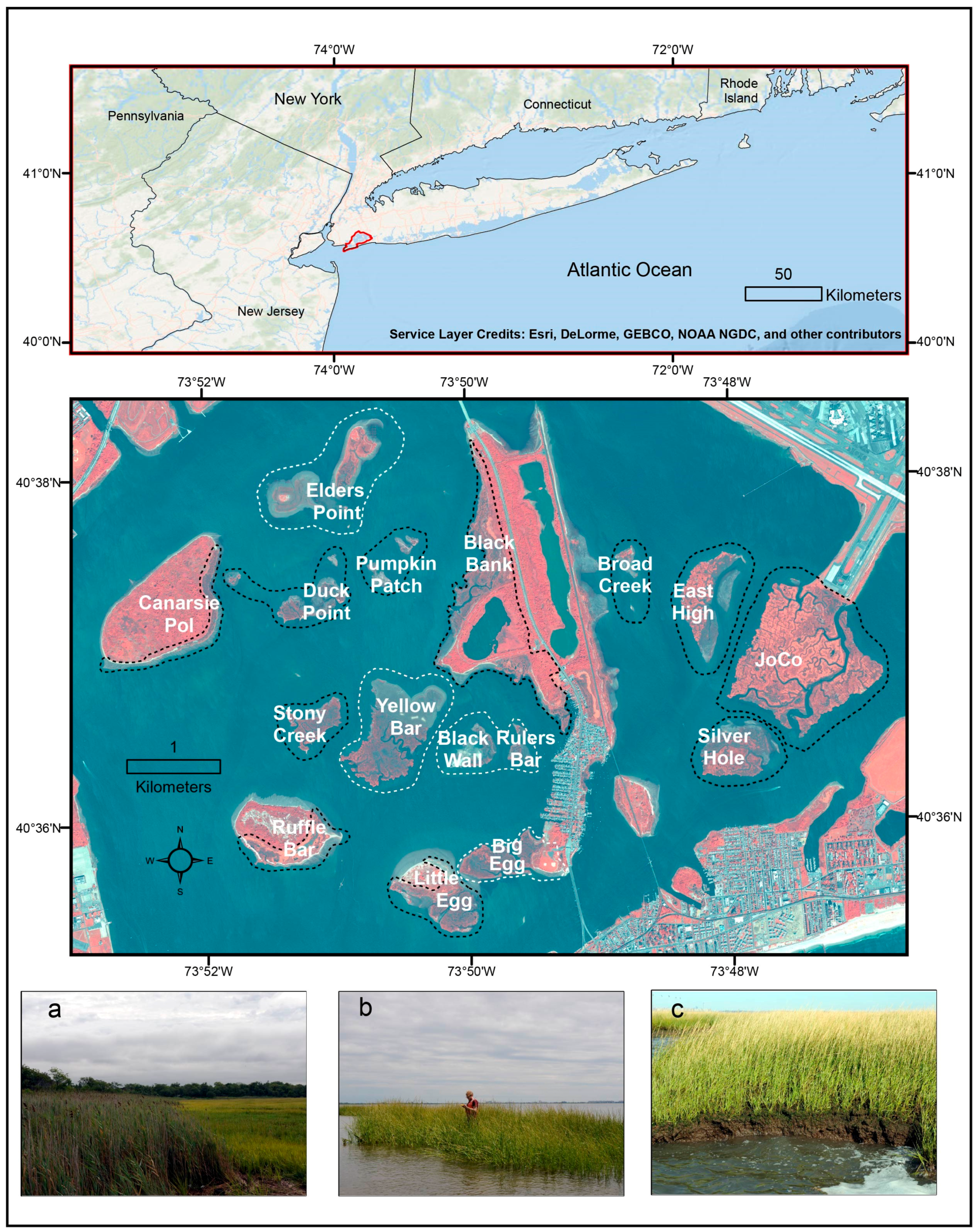
2.1. Study Area

Jamaica Bay is an urban estuary residing within the New York City boroughs of Brooklyn and Queens. Kings County, synonymous with Brooklyn, is the most populated county in New York State [13]. Approximately 3704 ha of the Bay are managed by the National Park Service as Jamaica Bay National Wildlife Refuge, a subunit of Gateway National Recreation Area (Figure 1). The region has a humid continental climate with a mean temperature of approximately 10 °C. Over the last 150 years, anthropogenic impacts to Jamaica Bay have been extensive. The Bay’s volume has increased 350% while surface area fell by approximately 4856 ha [14]. In 2005, Waste Water Treatment Plants serving 1,610,990 people discharged into Jamaica Bay [15]. Beginning in 2003, salt marsh islands including Big Egg, Yellow Bar, Rulers Bar, Black Bar, and Elders Point East and West (Figure 1) have undergone salt marsh restoration. After restoration, sites were monitored in situ for 5 years [4]. These marsh restoration projects involved the deposition of dredge sediment from channels in the Bay onto the marsh surface then the transplanting and seeding of salt marsh vegetation [16].

2.2. Remote Sensing Data

High spatial resolution Quickbird-2 and Worldview-2 data were employed for salt marsh mapping and change analysis. The spatial resolutions of Worldview-2’s multispectral and panchromatic sensors are 1.85 m and 0.42 m, respectively; Quickbird-2’s resolutions are 2.6 m and 0.62 m, respectively. The Worldview-2 sensor collects eight spectral bands including the Coastal Blue, Blue, Green, Yellow, Red, Red Edge, Near Infrared 1 (NIR1), and Near Infrared 2 (NIR2). The Coastal Blue, Yellow, Red Edge, and NIR2 spectral bands of Worldview-2 have been shown to increase the accuracy of wetland vegetation classification [17]. This study used Quickbird-2 imagery data acquired on 10 September 2003 and 9 September 2008, and Worldview-2 data acquired on 15 September 2012 and 19 September 2013. The imagery data were geo-rectified to the 2013 imagery. The data were also atmospherically corrected to top of atmosphere reflectance.

This study uses object-based image analysis (OBIA) which first divides an image into objects, using a segmentation algorithm, and then classifies those objects based on their spectral and spatial attributes [18]. Object-based change detection (OBCD) utilizes image objects to conduct a change analysis between multiple time periods. The change analysis can be conducted with object attributes, classified objects, multi-temporal image objects, or a hybrid of these techniques [19]. This study compared the classified 2003, 2008, 2012 and 2013 objects to understand restoration and Hurricane Sandy’s impact on wetlands within Jamaica Bay.

2.3. Segmentation

An important component of OBIA classifications is the determination of segmentation scale, which determines the size and similarity of resulting image objects, and parameterization, i.e., the inclusion of texture [20]. Texture is the use of a moving window to quantify measures that represent ideas such as coarseness and roughness [19]. This study arrived at an appropriate segmentation scale with the comparison of multiple segmentation scales for each time period to maximize intra-segment homogeneity and intersegment heterogeneity [21,22]. The parameterization of the resulting image objects included spectral values, texture, geospatial attributes, upland data, vegetation indices, and neighborhood and scene difference attributes (described in Section 2.4). Segmentation scale is the key to accurately mapping a landscape. Scale parameters can be arrived at through “trial-and-error”. However, this method risks determining an inappropriate segmentation scale. Over or under segmenting an image can result in lower classification accuracy [23]. In addition, segmentation scale can impact the land cover classes that can be accurately mapped [20]. This study used the mean shift clustering approach to determine segmentation. Mean shift is a non-parametric segmentation algorithm which groups pixels based on their spectral mean in a feature space. The algorithm has improved accuracy when compared to other clustering techniques [24,25]. Mean shift considers a spectral radius in the feature space as the scale parameter, which results in a hierarchical relationship between segmentation scales [26]. These factors make the algorithm suitable for multiscale segmentation.

There are different methods for assessing the quality of segmentation. This study assessed segmentation scales with an index of intra-segment homogeneity and intersegment heterogeneity [21]. Intersegment heterogeneity was assessed through computation of Global Moran’s I that were normalized and then combined with the intra-segment homogeneity, as determined by normalized area controlled variance, to create a single parameter measuring segmentation quality [22]. The mean shift segmentation parameters that were determined were minimum size and spectral radius. Minimum size refers to the fewest number of pixels that can compose a segment, and spectral radius is the distance in the feature which a pixel must be within to merge into the segment. Each image date was tested with the parameters from 5 to 50 spectral radii in increments of 1 and minimum size from 5 to 50 in increments of 5. Appropriate segmentation scale for the Worldview-2 2012 data was determined to be a spectral radius of 15 and a minimum size of 5. The 25% most over segmented objects were segmented again at a quantitatively determined appropriate scale of spectral radius 20 and minimum size 5. The same was done for 25% most under segmented objects, for which the appropriate scale was spectral radius 6 and minimum size 5. The appropriate scale for the Worldview-2 2013 data was determined to be spectral radius 22 and minimum size 20. The 25% most over segmented objects were segmented again at a quantitatively determined appropriate scale of spectral radius 27 and minimum size 5. The 25% most under segmented objects were re-segmented at a scale of spectral radius 7 and minimum size 5. The Quickbird-2 data were segmented at a spectral radius of 8 and a minimum size of 20 no additional levels of segmentation were done as this scale adequately captured the landscapes and spectral complexity of the Quickbird-2 data.

The classification was conducted with the Random Forest classifier. Random Forest is a non-parametric ensemble learning algorithm that has been demonstrated to achieve appropriate classification accuracy in a variety of landscapes [27,28,29]. The 9 classes used in this study included 6 from a previous study of the Bay [8]. These classes included water, mudflat, sand, high marsh, patchy S. alterniflora, and S. alterniflora (>50% vegetation cover). The two S. alterniflora classes were based on percent cover with patchy being between 10% and 49% vegetation cover and S. alterniflora (>50% vegetation cover) being above 50%. Salicornia species are present within the Bay as a small component of the salt marsh [30], and were not prevalent enough to classify on their own. Additional classes included in this study are wrack, upland vegetation, Phragmites, and shadow, however shadow was removed with a decision tree post-classification. The 2003 classification did not include wrack due to the limited separability of the class in those images. These additional classes were included to expand our understanding of the Bay and inform management decisions.

2.4. Object Attributes

Spectral attributes included the mean and standard deviation of all available spectral bands. The spatial variables computed were perimeter, area, and nodes. The panchromatic band was utilized to create Grey-Level Co-Occurrence Matrix (GLCM) textural measurements, including inverse difference moment, entropy, contrast, correlation, and uniformity. GLCM and other texture measures have been shown to improve classification accuracies in both Very High Resolution image classification [31] and object-based wetland classification [32]. Red Edge-based vegetation indices, have been shown to more accurately discern differences between high density vegetation species [33]. In this study, Worldview Vegetation Index (WVVI), Worldview Water Index (WVWI), Red Edge-based NDVI, NDVI, and Soil Adjusted Vegetation Index (SAVI) were calculated after pan-sharpening due to its benefits for detecting small vegetation patches (formulas in

Table 1. Vegetation Indices, including Worldview-2 Vegetation Index, Worldview-2 Water Index, Red Edge Vegetation Index, Normalized Difference Vegetation Index and Soil Adjusted Vegetation Index.

WVVI	WVWI	NDVI	Red Edge Vegetation Index	SAVI
$\frac{\left(NIR2-Red\right)}{\left(NIR2+Red\right)}$	$\frac{\left(CB-NIR2\right)}{\left(CB+NIR2\right)}$	$\frac{\left(NIR-Red\right)}{\left(NIR+Red\right)}$	$\frac{\left(NIR-RedEdge\right)}{\left(NIR+RedEdge\right)}$	$\frac{\left(NIR-RED\right)\times \left(1+L\right)}{\left(NIR+RED+L\right)}$

) [34]. Ancillary data included an upland GIS layer created from a geomorphological map of Jamaica Bay [35] and Digital Elevation Model (DEM) derived from 2014 Topo-bathymetric Light Detection and Ranging [36].

Object neighborhoods, those objects that share a border with an object, and weights were calculated to determine the neighborhood difference of the mean spectral, textural and vegetation index attributes giving additional spatial context to the data [37]. The final Worldview-2 image objects had 79 attributes including 3 spatial attributes, 18 texture attributes, 32 spectrally derived attributes, 7 elevation based, 18 vegetation index, and a binary upland variable (

Table A3. Object parameters used in OBIA for 2012 and 2013 Worldview-2 imagery classification.

Variable Type	Variable Name	Variable Importance
Elevation	DEM mean	47
Elevation	DEM Standard Deviation (SD)	4
Elevation	DEM min	4
Elevation	DEM max	57
Elevation	DEM range	3
Elevation	DEM sum	17
Geospatial	Node points	0
Geospatial	Perimeter	1
Geospatial	Area	1
Ancillary	Upland binary layer	36
Spectral	Coastal blue mean	24
Spectral	Coastal blue SD	2
Spectral	Blue mean	31
Spectral	Blue SD	1
Spectral	Green mean	28
Spectral	Green SD	0
Spectral	Yellow Mean	26
Spectral	Yellow SD	1
Spectral	Red mean	29
Spectral	Red SD	1
Spectral	Red edge mean	46
Spectral	Red Edge SD	3
Spectral	NIR1 mean	58
Spectral	NIR2 Mean	67
Spectral	Coastal blue mean neighborhood difference	0
Spectral	Blue mean neighborhood difference	0
Spectral	Green mean neighborhood difference	1
Spectral	Yellow mean neighborhood difference	1
Spectral	Red mean neighborhood difference	1
Spectral	Red edge mean neighborhood difference	0
Spectral	NIR1 mean neighborhood difference	0
Spectral	NIR2 mean neighborhood difference	0
Spectral	Coastal blue mean neighborhood difference	16
Spectral	Blue mean scene difference	20
Spectral	Green mean scene difference	30
Spectral	Yellow mean scene difference	25
Spectral	Red mean scene difference	33
Spectral	Red edge mean scene difference	54
Spectral	NIR1 mean scene difference	51
Spectral	NIR2 mean scene difference	73
Spectral	NIR1 SD	4
Spectral	NIR2 SD	1
Texture	Correlation mean	0
Texture	Entropy mean	0
Texture	Inverse Difference Moment(IDM) mean	0
Texture	Uniformity mean	0
Texture	Contrast mean	0
Texture	Correlation mean neighborhood difference	0
Texture	Entropy mean neighborhood difference	0
Texture	IDM mean neighborhood difference	0
Texture	Uniformity mean neighborhood difference	0
Texture	Contrast mean scene difference	0
Texture	Correlation mean scene difference	0
Texture	Entropy mean scene difference	0
Texture	IDM mean scene difference	0
Texture	Uniformity mean scene difference	0
Texture	Contrast SD	0
Texture	Entropy SD	0
Texture	IDM SD	0
Texture	Uniformity SD	0
Vegetation Index	REVI mean	26
Vegetation Index	WVVI mean	74
Vegetation Index	WVWI mean	93
Vegetation Index	REVI mean neighborhood difference	0.9
Vegetation Index	WVVI mean neighborhood difference	1
Vegetation Index	WVWI mean neighborhood difference	1
Vegetation Index	REVI mean scene difference	12
Vegetation Index	WVVI mean scene difference	66
Vegetation Index	WVWI mean scene difference	100
Vegetation Index	REVI SD	0
Vegetation Index	WVVI SD	0
Vegetation Index	WVWI SD	0
Vegetation Index	SAVI range	0
Vegetation Index	SAVI mean	39
Vegetation Index	SAVI SD	0
Vegetation Index	NDVI range	0
Vegetation Index	NDVI mean	50
Vegetation Index	NDVI SD	0

). The Quickbird-2 image objects had additional attributes including tasseled cap values but no Red Edge based NDVI.

2.5. Accuracy Assessment

The accuracy assessments were conducted for each classification by generating equalized random points. The number of points to generate was calculated with following equation [38].

$$N=\frac{B{{\displaystyle \prod }}_i(1-{{\displaystyle \prod }}_i)}{b_i^2}$$

where $B$ is the Chi-squared distribution with 1 degree of freedom for the target error divided by the number of classes, ${\displaystyle \prod }_i$ is the percent land cover of the most prevalent class and $b$ is the desired confidence interval of that class. The calculation required over 750 test points to fulfill the accuracy assessment. The final test dataset was composed of 765 test points. The objects were classified by the user based on Worldview-2, Quickbird-2, and Google Earth historic imagery from each time period. Overall accuracy, the Kappa statistic, producer’s accuracy, and user’s accuracy were calculated to analyze the confusion matrix results [39,40]. The study site was visited in 2014 and 2015 to verify the characteristics of the landscape and collect field reference data. The training samples and objects were extracted from Worldview-2 and Quickbird-2 imageries in combination with expert knowledge from the field visits. Land cover points were collected on each of the field visits. The point locations included areas in West Pond, Black Bank, Yellow Bar, JoCo, Elders Point, Canarsie Pol, and East High. The points were navigated to with a Trimble XH and the areas dominate vegetation community was verified.

2.6. Statistical Analysis

The finished classifications were utilized to determine change rates (ha/year) in the three time periods 2003–2008, 2008–2012 and 2012–2013. Jamaica Bay’s unique salt marsh structure of individual islands led to their use for statistical analysis. The paired Wilcoxon signed rank test was utilized to test the differences between wrack extent throughout the Bay in 2008, 2012 and 2013 (

Table A1. Land cover extent of salt marsh islands (ha).

Marsh	Year	Mudflat	Sand	S. alterniflora (50% > Vegetation Cover)	Patchy S. alterniflora	High Marsh	Water	Wrack	Upland Vegetation	Phragmites
Pumpkin Patch	2003	0.9	0.0	1.3	1.6	0.0	30.3	-	0.0	0.0
	2008	2.1	0.0	0.8	0.7	0.1	28.9	0.1	0.0	0.0
	2012	3.3	1.4	0.2	0.3	0.0	27.4	0.1	0.0	0.0
	2013	0.7	0.1	0.2	0.2	0.0	31.4	0.0	0.0	0.0
Canarsie Pol	2003	3.9	0.9	5.4	2.5	1.8	12.6	-	1.2	1.7
	2008	3.9	0.6	5.1	1.6	2.1	12.9	0.7	0.6	2.5
	2012	9.5	1.8	4.2	3.3	0.1	6.2	0.7	0.7	3.4
	2013	7.2	1.8	5.2	1.1	0.3	9.4	0.3	0.3	4.2
Stony Creek	2003	3.9	0.0	5.4	4.8	0.2	41.7	-	0.0	0.0
	2008	4.1	0.0	6.4	2.9	1.2	21.8	0.1	0.0	0.0
	2012	5.4	0.3	6.3	2.3	0.0	22.1	0.0	0.0	0.0
	2013	3.1	0.1	7.5	1.6	0.0	24.2	0.0	0.0	0.0
Little Egg	2003	7.7	0.7	7.1	6.1	0.8	22.6	-	0.0	1.6
	2008	8.2	1.7	9.5	4.0	3.3	18.7	1.8	0.0	0.5
	2012	10.8	4.4	10.3	4.5	0.3	13.8	1.1	0.0	0.2
	2013	6.7	4.8	13.4	2.2	0.6	16.8	0.1	0.0	0.7
Big Egg	2003	8.5	0.1	7.3	5.3	1.4	15.4	-	0.1	0.6
	2008	5.8	0.1	11.9	3.6	2.5	11.7	0.3	0.1	0.6
	2012	12.0	0.3	8.5	4.8	0.2	8.6	0.5	0.0	0.4
	2013	5.9	0.2	12.6	3.2	0.3	12.3	0.1	0.0	0.8
Black Wall + Rulers Bar	2003	2.9	0.0	1.5	2.6	0.0	47.4	-	0.0	0.0
	2008	5.1	0.0	2.1	2.3	1.0	43.9	0.0	0.0	0.0
	2012	8.3	2.9	1.2	1.5	0.0	40.4	0.0	0.0	0.0
	2013	17.1	1.1	0.9	0.3	0.0	34.9	0.0	0.0	0.0
Black Bank	2003	9.5	1.1	27.4	11.5	5.4	27.2	-	19.6	4.8
	2008	8.9	1.7	27.0	6.7	5.0	20.3	3.2	19.7	7.7
	2012	19.3	2.7	25.7	6.8	2.4	15.5	3.0	19.2	5.6
	2013	8.6	2.3	29.4	3.5	3.5	24.7	1.	18.8	8.4
Duck Point	2003	4.6	0.1	3.9	2.6	0.6	40.2	-	0.0	0.0
	2008	2.6	0.1	4.1	4.3	0.1	49.7	0.0	0.0	0.0
	2012	10.4	1.0	3.2	2.1	0.0	35.3	0.2	0.0	0.0
	2013	4.3	0.2	3.8	1.3	0.0	42.6	0.0	0.0	0.0
Broad Creek	2003	1.3	0.0	1.4	0.7	0.6	33.9	-	0.0	0.1
	2008	1.8	0.2	0.8	0.2	0.4	27.4	0.2	0.0	0.0
	2012	2.7	0.4	0.6	0.2	0.1	26.9	0.1	0.0	0.0
	2013	1.3	0.2	0.8	0.2	0.1	28.4	0.0	0.0	0.1
East High	2003	10.5	0.1	14.3	5.8	3.0	49.6	-	0.0	0.0
	2008	15.1	0.1	12.5	3.1	4.0	48.2	0.3	0.0	0.0
	2012	18.7	0.7	11.8	1.6	2.6	47.7	0.2	0.0	0.0
	2013	5.1	0.3	12.7	1.7	2.8	60.6	0.0	0.0	0.0
JoCo	2003	11.1	0.1	72.4	20.1	37.5	83.6	-	0.1	1.3
	2008	11.9	0.1	74.5	11.8	44.6	79.6	3.1	0.0	0.4
	2012	18.5	0.3	82.0	6.5	35.5	80.9	2.2	0.0	0.1
	2013	12.6	0.1	90.7	7.1	29.8	85.1	0.5	0.0	0.0
Elders Point West	2003	2.8	0.2	1.2	0.7	0.2	40.1	-		0.1
	2008	3.9	0.4	1.0	0.5	0.5	38.4	0.1	0.0	0.1
	2012	15.5	0.7	0.5	2.8	0.0	25.3	0.1	0.0	0.1
	2013	14.0	0.3	2.2	2.4	0.2	25.5	0.3	0.0	0.3
Yellow Bar	2003	18.2	0.0	12.9	12.6	0.8	67.9	-	0.0	0.0
	2008	23.1	0.0	17.5	9.0	1.8	56.4	0.1	0.0	0.0
	2012	43.0	0.7	12.5	5.6	0.1	46.0	0.1	0.0	0.0
	2013	33.7	0.1	18.7	7.5	0.1	48.0	0.0	0.0	0.0
Silverhole	2003	11.1	0.0	11.8	8.0	0.9	40.7	-	0.0	0.0
	2008	12.6	0.0	15.2	3.3	1.1	25.5	0.2	0.0	0.1
	2012	16.6	0.4	12.9	3.0	0.2	24.5	0.3	0.0	0.0
	2013	13.3	0.2	14.5	3.4	0.3	26.1	0.0	0.0	0.0
Ruffle Bar	2003	4.1	1.9	7.7	1.8	6.4	12.0	-	0.1	3.0
	2008	3.7	2.5	6.3	0.8	7.7	11.3	2.1	0.0	0.5
	2012	7.7	3.4	6.5	1.5	5.2	7.4	1.0	2.2	0.0
	2013	44.6	3.3	6.1	0.7	5.1	11.1	0.2	3.9	0.0
Elders Point East	2003	2.3	0.2	2.0	1.5	0.2	68.0	0.0	0.1	0.2
	2008	5.4	0.3	11.0	1.0	0.7	54.4	0.7	0.2	0.6
	2012	11.4	1.2	7.5	1.1	0.5	51.1	1.0	0.3	0.1
	2013	9.6	1.0	8.2	0.7	0.9	53.1	0.2	0.1	0.6

). These extents were for each island for each year. The difference between percent change (Δ%/year) of restored and natural salt marsh from 2012 to 2013 was tested with a student’s t-test. Comparing all natural salt marshes to those where restoration was completed by the data acquisition in 2012. Before utilizing the t-test, normality was tested with the Shapiro–Wilkes statistic, which indicated normality could not be rejected with p values = 0.37 and 0.80 for restoration and natural, respectively. The natural salt marsh islands for all time periods were used to compare change rates (ha/year) with paired t tests. The time periods were tested with Shapiro–Wilkes for normality finding p values of 0.54, 0.29, 0.43 and 0.19 for 2003–2008, 2008–2012, 2012–2013 and 2003–2012 respectively. Linear regressions were used to understand the impact of salt marsh extent, latitude, and longitude on combined high marsh and both classes of S. alterniflora change rates (ha/year). Latitude and longitude were determined from the center point of each salt marsh island.

3. Results

The landscape was mapped accurately throughout the classification results (accuracies of 85.63, 85.2, 90.46 and 92.55 for 2003, 2008, 2012 and 2013, respectively). The overall accuracies were further analyzed by producer’s accuracy and user’s accuracy (

Table 2. Accuracy assessment analysis (producer’s, user’s, and overall accuracy).

	Year	Mudflat	Sand	S. alterniflora (>50% Vegetation Cover)	Patchy S. alterniflora	High Marsh	Water	Wrack	Upland Vegetation	Phragmites	Overall Accuracy (%)
Producer’s Accuracy (%)	2003	90.12	98.70	70.73	71.43	82.93	97.50	-	92.68	81.01	85.63
	2008	89.53	83.16	76.84	80.23	85.54	96.59	77.46	91.86	85.33	85.23
	2012	89.53	90.70	95.06	88.37	98.77	98.84	80.43	91.46	82.35	90.46
	2013	92.31	92.77	92.05	98.75	91.86	100.0	89.41	94.05	82.35	92.55
User’s Accuracy (%)	2003	91.25	95.00	72.50	68.75	85.00	97.50	-	95.00	80.00	85.63
	2008	90.59	92.94	85.88	81.18	83.53	100.0	64.71	92.94	75.29	85.23
	2012	90.59	91.76	90.59	89.41	91.12	100.0	87.06	88.24	82.35	90.46
	2013	98.82	90.59	95.29	92.94	92.94	97.65	89.41	92.94	82.35	92.55

). The 2003 data had an adequate overall accuracy of 85.6%, with vegetation classes exhibiting the lowest accuracies (Table 2). This led to a focus on comparing vegetated salt marsh and non-vegetated areas as most of the error was between the multiple classes of salt marsh. The three classes of vegetated (S. alterniflora classes, high marsh, and Phragmites), non-vegetated (water, mudflat, sand, and wrack) and upland were used for comparisons between periods unless stated otherwise. These three classes had overall accuracies of 96.09, 93.46, 93.46 and 96.73 for 2003, 2008, 2012 and 2013, respectively.

3.1. Wetland Change

The 2003 and 2013 classifications were compared to determine change between all classes (

Table 3. Change between 2003 and 2013 (ha). Areas that had no change between the two dates are in grey.

		2013
	Class	Water	Mudflat	Sand	S. alterniflora (50% > Vegetation Cover)	Patchy S. alterniflora	Phragmites	High Marsh	Upland	Total 2003 Area (ha)
2003	Water	485.5	66.3	3.8	12.6	6.7	0.1	0.8	0.0	651.4
	Mudflat	19.4	43.3	3.5	22.4	11.1	0.3	0.7	0.0	102.2
	Sand	0.4	1.0	2.7	0.5	0.2	0.2	0.1	0.1	5.7
	S. alterniflora (50% > vegetation cover)	13.4	16.5	2.5	115.6	10.1	6.1	16.4	1.0	183.4
	Patchy S. alterniflora	11.2	19.3	0.8	46.4	8.9	0.4	2.3	0.1	89.9
	Phragmites	0.1	0.2	1.5	2.6	0.8	5.5	1.0	1.1	14.0
	High Marsh	2.3	1.4	0.8	26.6	1.3	3.0	22.8	0.5	59.2
	Upland	0.00	0.2	0.3	0.2	0.2	3.2	0.1	16.5	21.3
	Total 2013 Area (ha)	535.7	148.0	16.1	226.7	36.8	19.0	44.0	19.3

). From 2003 to 2013, 54.9 ha of sand, mudflat and water were converted into salt marsh. However, during that same period, 70.7 ha of high marsh and S. alterniflora were converted into sand, mudflat, or water. Salt marsh vegetation gains occurred in restoration sites, however, these were exceeded by losses in areas not subject to intervention (Figure 2). Elders Point East and West were restored during the study period, an example of restoration driven change in the Bay (Figure 3). West Pond was breached during Hurricane Sandy and areas of freshwater wetland and upland vegetation shifted to mudflat (Figure 4). From 2003 to 2013, 21 ha of salt marsh were lost, including both S. alterniflora classes, high marsh, and Phragmites. Smaller salt marshes such as Duck Point and Pumpkin Patch nearly disappeared (Figure 1 and Figure 2).

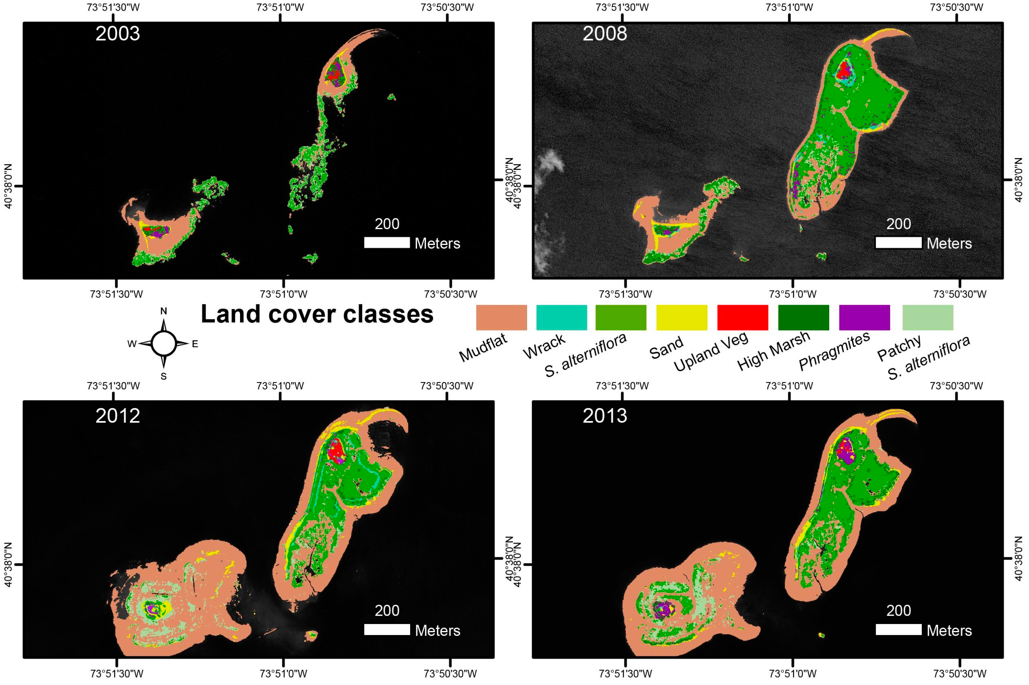
3.2. Restored Islands: 2003–2013

Elders Point East and West were restored in 2006 and 2010, respectively [4]. These islands were not being actively restored during the 2012–2013 period, however they did increase in salt marsh extent (Table A1). From 2012 to 2013, Yellow Bar, Rulers Bar, and Black Wall were the focus of significant restoration. In 2013, Yellow Bar added 8.0 ha of salt marsh vegetation, but had a negligible change in extent from 2003 to 2013. Yellow Bar’s restoration process also added approximately 15 ha of mudflat, however, this does not account for the 32.5 cm higher tide in 2003 as determined from the Sandy Hook tidal gauge [41]. From 2003 to 2008, restoration of Big Egg and Elders Point East were completed, resulting in increases in salt marsh extent of 4.0 and 9.5 ha, respectively. Big Egg subsequently lost 4.7 ha of salt marsh extent between 2008 and 2012.

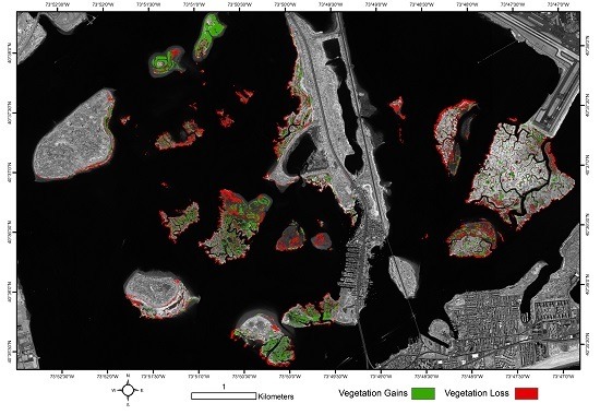
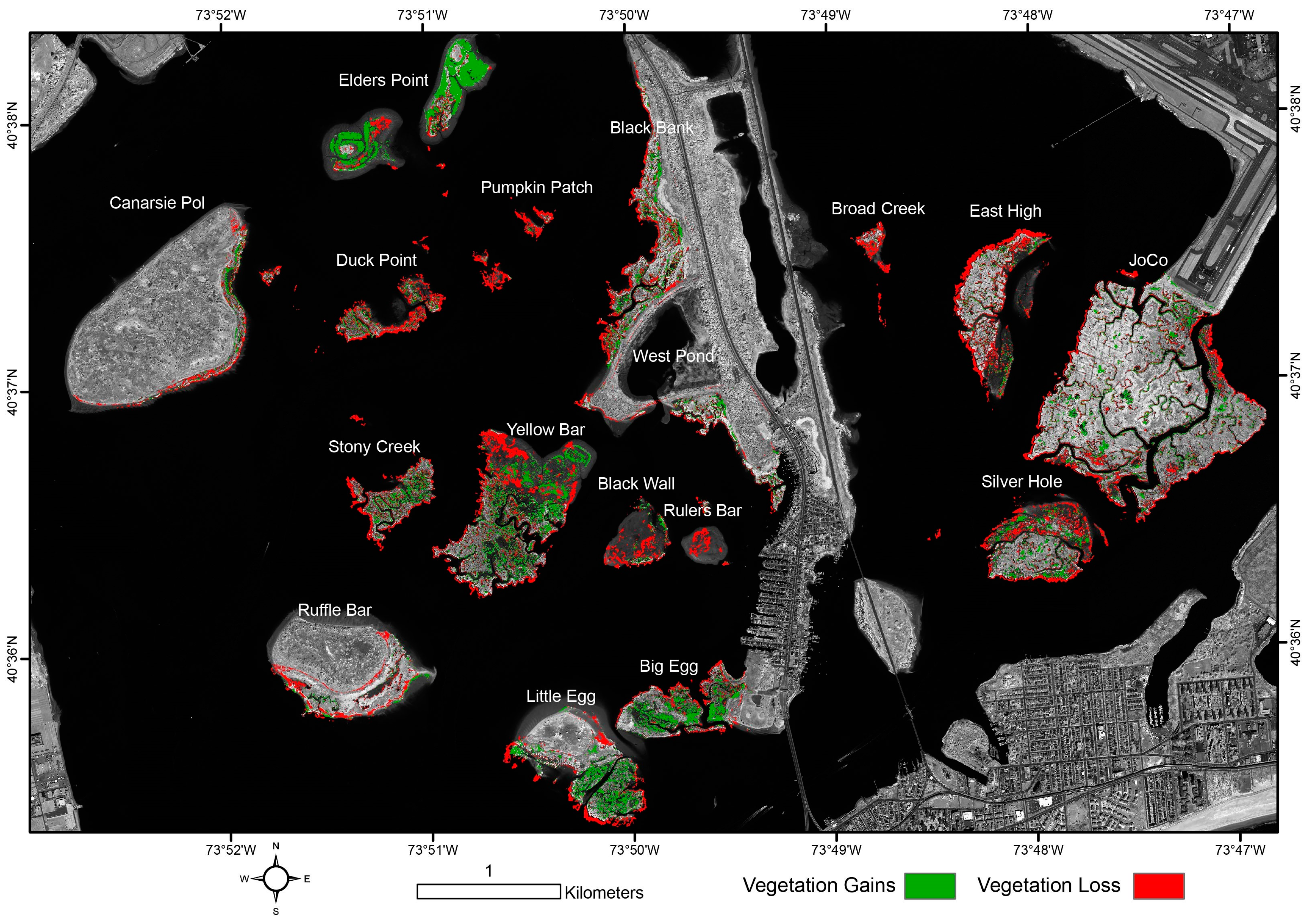
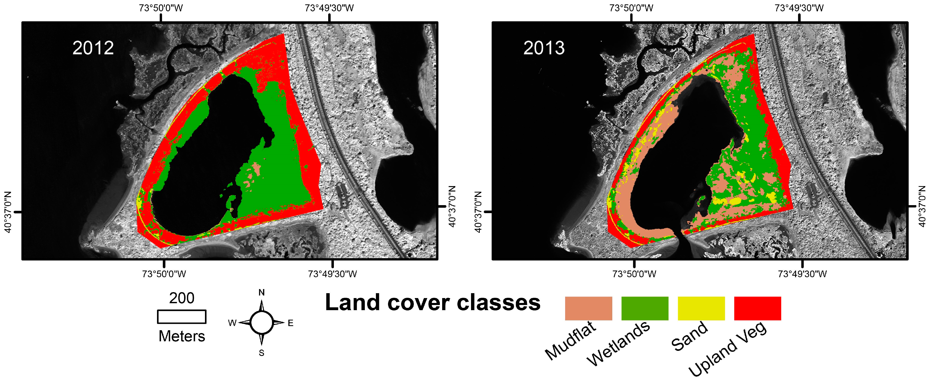
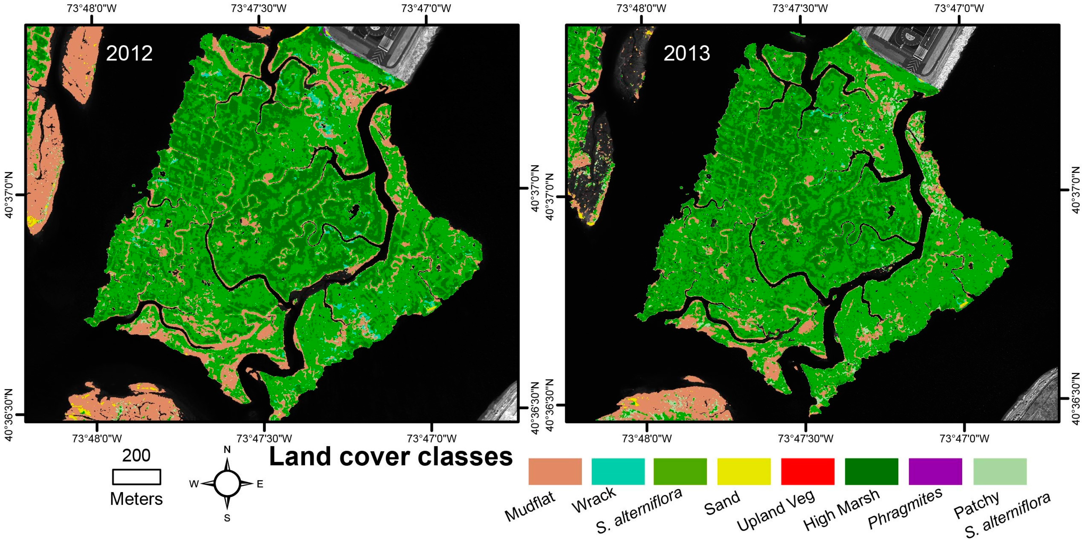
3.3. Impact of Hurricane Sandy

West Pond (Figure 2) is a retention pond created during the construction of the Cross Bay Boulevard and an important resource for migratory birds [42] (Figure 4). Hurricane Sandy breached West Pond, resulting in saltwater intrusion into the freshwater environment [43]. Prior to this breach, West Pond’s wetlands were dominated by Phragmites australis. The area represents the most drastic change from Hurricane Sandy; alterations to the upland and freshwater wetlands are evident (Figure 4 and

Table 4. Change of land cover classes between 2012 and 2013 for West Pond area.

		2012
	Change or No Change Areas (ha)	Mudflat	Sand	Wetland	Water	Upland Veg.	Post-Storm Total
2013	Mudflat	0.3	0.0	4.4	1.0	2.5	8.3
	Sand	0.0	0.4	0.9	0.0	0.4	1.7
	Wetland	0.0	0.0	7.4	0.0	2.8	10.2
	Water	0.1	0.0	0.4	16.9	0.1	17.5
	Upland Veg.	0.0	0.0	0.2	0.0	5.8	6.0
	Pre-storm Total	0.4	0.5	13.3	17.9	11.5

).

Between 2003 and 2013, the JoCo site lost salt marsh vegetation going from 131.2 ha to 127.6 ha. However, from 2012 to 2013 vegetation increased (Table A1). This increase in vegetation was accompanied by a reduction in wrack across the Bay compared to both 2008 (W₁₅ = 110, p < 0.003) and 2012 (W₁₅ = 113, p = 0.0011). The area of wrack was reduced after Hurricane Sandy going from 2.2 ha to 0.5 ha. This in part accounts for the 3.6 ha increase of salt marsh vegetation observed in JoCo. The 2008 and 2012 classifications of JoCo had only 0.2 ha of overlapping wrack.

JoCo salt marsh was the most stable during the time period analyzed (Table A1). The restoration salt marshes in 2012–2013 had a larger percentage increase of salt marsh vegetation than natural salt marshes (t₄, p = 0.041). The natural salt marshes in 2012–2013 demonstrated a larger positive change than 2003–2008 (t₁₀ = 2.366, p = 0.039), 2008–2012 (t₁₀ = 2.6893, p = 0.022) and 2003–2012 (t₁₀ = 2.5434, p < 0.03). The 2008–2012 and 2003–2008 change rates were also significantly different (t₁₀ = 2.8012, p < 0.02) (

Table A2. Salt marsh change rates for 2003–2008, 2008–2012 and 2012–2013 (ha/year).

Marsh	2003–2008	2008–2012	2012–2013
Pumpkin Patch	−0.3	−0.3	−0.1
Canarsie Pol	−0.01	−0.1	−0.2
Stony Creek	0.03	−0.5	0.5
Little Egg	0.3	−0.5	1.5
Big Egg	0.8	−1.2	2.9
Black wall + Rulers Bar	0.2	−0.7	−1.5
Black Bank	−0.5	−1.5	4.3
Duck Point	0.3	−0.8	−0.1
Broad Creek	−0.3	−0.1	0.2
East High	−0.7	−0.9	1.3
JoCo	0.0	−1.7	3.5
Elders Point West	−0.02	0.3	1.6
Elders Point East	1.9	−1.0	1.1
Yellow Bar	0.4	−2.5	8.0
Silverhole	−0.2	−0.9	2.2
Ruffle Bar	−0.7	−0.5	−1.4

). However, 2012–2013 was the only period when a mean increase in natural salt marsh vegetation was observed.

We analyzed the natural salt marshes yearly change rates (ha/year) by linear regression for each time period. The only time period where salt marshes towards the eastern side of the Bay tended to gain vegetation was 2012–2013 (F_1,9 = 22.21, p < 0.002 and R² = 0.7116). Larger salt marshes in 2012 tended to gain vegetation in 2012–2013 (F_4,6 = 13.93, p < 0.036 and R² = 0.9028). From 2008 to 2012, larger salt marshes in 2008 tended to lose more vegetation (F_4,6 = 6.83, p < 0.011 and R² = 0.8199). From 2003 to 2008, no relationship was found between salt marsh extent and change (F_4,6 = 0.75, p = 0.41 and R² = 0.33). The switch in the direction of this relationship demonstrates different processes dominating the Bay between 2008–2012 and 2012–2013.

3.4. Accuracy Assessment

Confusion matrices were utilized to determine the performance of each of the classifications. The 2012 and 2013 classifications performed well in all vegetation classes of most interest including S. alterniflora and high marsh (Table 2). The lowest performing class was Phragmites, which is a difficult to classify land cover with overlap between many of the other classes spectrally and spatially. The 2003 and 2008 classifications had low salt marsh vegetation accuracy due to confusion between the salt marsh vegetation types. The 2003 and 2008 error was mitigated by focusing our analysis on change in vegetation not changes in particular types of vegetation. Overall, the Worldview-2 data were better suited for the specificity of this classification.

4. Discussion

Since the 1950s, salt marsh vegetation in Jamaica Bay has been in rapid decline and, in the early 2000s, restoration was deemed necessary to maintain the salt marsh. This study and past estimates of salt marsh change were compared to better understand vegetation trends. From 1989 to 2003, there was an estimated 13.4 ha of yearly loss [5]. From 2003 to 2013, a yearly loss of 2.1 ha was observed. The long-term rate of salt marsh loss in the Bay slowed due in part to restoration, however, both tidal stage and nutrient inputs may have influenced this result.

The 2003 and 2013 data were collected at a tidal stage of −0.129 m and −0.454 m (North American Vertical Datum) [41]. Between 2003 and 2013, the larger salt marsh islands appeared to gain vegetation in the interior and lose salt marsh on the edges (Figure 2). However, the difference in tidal stage of the data could be responsible for some vegetation increases between the two dates. The tidal stage of the 2012 data was −0.577 NAVD [41]. The small tidal difference in 2012 and 2013 could result in less inundated vegetation in 2012. Tidal stage may have influenced the larger trends from 2003 to 2013, but was not a factor in the vegetation increase from 2012 to 2013. The impact of the tides on mapping salt marsh in Jamaica Bay should be further explored to account for this uncertainty.

Since the mid-2000s, the Bay has had a 30% reduction in nitrogen load [44]. Nutrient enrichment in salt marsh systems can lead to creek bank collapse and conversion to mudflat [6]. The Waste Water Treatment Plants in Jamaica Bay account for 89% of all nitrogen inputs into the Bay; due to the Bay’s currents, the highest nitrogen concentrations were in the south and eastern sides of JoCo [15]. The different responses of salt marshes in the Bay to nutrient enrichment was partly explained by lower elevation marshes having longer periods of inundation increasing decomposition and loss of organic matter [45]. The nitrogen load reduction coincided with the slowing of salt marsh loss, however, the impact is unknown and in situ analysis would be necessary to explore this possible connection.

4.1. Restoration

In 2003, the first salt marsh restoration in Jamaica Bay began at Big Egg. The project utilized dredge sediment to increase marsh elevation and then S. alterniflora plugs were planted 50 cm apart [17]. In 2006, Elders Point East’s elevation was increased with dredge sediment and then vegetated with both plugs and hummock relocation, the removal followed by placement of the entire salt marsh platform on areas of restored elevation [4]. The hummock relocation saves salt marsh that would be covered in dredge sediment, and provides vegetation to the restored area. In 2010, the elevation of Elders Point West was increased with dredge sediment and vegetated with a combination of hummock relocation, planting of high marsh species, seeding of S. alterniflora, and a test site with no planting [4]. In early 2012, Yellow Bar was restored with dredge material and vegetated with a mix of hummock relocation and salt marsh seeding [46]. In fall 2012, the elevation of Rulers Bar and Black Wall was increased with dredge sediment. In June 2013, a community effort added vegetation to these islands with plugs [46]. This decade of restoration coincided with our study, and resulted in the evaluation of this methodology for understanding restoration.

Black Wall and Rulers Bar were restored between 2012 and 2013. These marsh islands showed no evidence of revegetation at the time of the 2013 mapping. The salt marsh vegetation of Black Wall and Rulers Bar was reduced from 2.7 to 1.2 ha while sand and mudflat increased from 11.2 to 18.2 ha. The loss of vegetation appeared to be connected with sediment deposition from restoration and lack of hummock relocation. However, the storm event could have exacerbated the loss. Rulers Bar lost nearly all salt marsh vegetation from 2012 to 2013 (Table A1). In June 2013, Plugs had been planted on Black Wall and Rulers Bar. However, the vegetation was sparse and classified as mudflat.

While restored salt marsh corresponded with a visual change, it may not represent a recovery of all the ecosystem services. Differences between natural and restored salt marshes include lower soil organic matter, insufficient nitrogen availability, stunted plant growth and increased susceptibility to herbivory [47]. Field studies in Jamaica Bay have demonstrated some differences between restored and natural salt marshes, including a high percent of sand and less soil organic matter in the first 10 cm of soil [45]. These differences and the unknown longevity of restored marshes are the reasons long-term monitoring is necessary. Big Egg and Elders Point East both demonstrated losses post restoration from 2008 to 2012, with a loss of 1.1 ha and 1.0 ha per year, respectively. Post-restoration losses demonstrate the need for further understanding of the underlying processes causing salt marsh loss in Jamaica Bay. The expected lifetime of a restored marsh could be estimated and used to inform management decisions.

Restoration planting occurred on Yellow Bar between the 2012 and 2013 data collections (

Table 5. Salt marsh restoration site, year, and extent [16,46].

Year	Salt Marsh	Area (ha)
2003	Big Egg	1.0
2006–2007	Elders Point East	16.2
2010	Elders Point West	16.2
2012	Yellow Bar	18.2
2013	Black Wall	6.1
2013	Rulers Bar	4.0

). The restoration process added elevation and S. alterniflora to the northern area of the site. The restoration resulted in vegetation increasing from 18.2 to 26.3 ha. Elders Point’s restoration was already complete in 2012, however, the combined vegetated extent of Elders Point East and West went from 13.0 to 14.5 ha. Restoration sites added vegetation in the post-storm growing season. Restoration sites did not appear to be negatively impacted by Hurricane Sandy. However, post-storm the Yellow Bar restoration required extensive repairs and replanting [46]. The storm impacted Yellow Bar at an early stage of restoration, which led to a slowing of the process. However, considerable vegetation was gained in the post-storm growing season.

4.2. Hurricane Sandy

The response of salt marshes to storm events vary and include net elevation increases leading to vegetation growth [48] and accretion varying with distance to an inlet [49]. The natural and restoration salt marshes responded differently to Hurricane Sandy. The analysis of natural salt marsh separated the restoration and storm impacts. In 2012–2013, larger salt marshes and those further from Rockaway inlet tended to gain vegetation. This is in agreement with past hurricane impacts which had a wide variation in sediment deposition and salt marsh response including edge erosion [50]. The large salt marshes may have been less impacted by Hurricane Sandy, and captured more of the accompanying sediment pulse.

The response of vegetation in Jamaica Bay to Hurricane Sandy depended on the location and the ecosystem. Saltwater intrusion into freshwater ecosystems is a major source of storm event derived vegetation loss; evident in both coastal wetland environments [51] and forests [52]. The survival and recovery of freshwater wetland vegetation depends on the species [53] and replanting of coastal forests can be limited by the increased soil salinity and herbivory [54]. These long-term impacts emphasize the importance of monitoring the West Pond breach. Post-storm, both freshwater wetland and upland vegetation lost extent declining from 13.3 ha to 10.2 ha and 11.5 ha to 6.0 ha, respectively (Table 4). There were 2.9 ha of change from upland vegetation to freshwater wetland, which can be understood as a loss of vegetation biomass but not a complete loss of vegetation. Excluding those areas, 5.9 ha of freshwater wetland were lost. The majority of vegetation lost became mudflat. The loss of upland vegetation suggests the approximate extent of saltwater intrusion into the upland areas around West Pond. The environmental assessment of the site has resulted in the decision to close the breach and restore the freshwater wetland environment [55]. This approach will create early successional habitat. Continued monitoring of West Pond is necessary to understand both the recovery of the freshwater ecosystem and unforeseen impacts of the management decision.

4.3. Wrack

Wrack is an important component of Jamaica Bay’s landscape as persistent wrack deposits, for over four months of time, have a negative impact on the growth rate of all the principal marsh species [56]. Storm events including hurricanes are understood as one of the causes of wrack accumulation [50]. Mapping wrack accumulation pre- and post-storm enabled the evaluation of both the deposition and movement of wrack within Jamaica Bay. Post-storm there was less wrack on the salt marsh than in 2008 and 2012. When examining JoCo, it appears areas of wrack moved towards the center of the marsh island (Figure 5). If the same pattern occurred in islands with upland, wrack would have moved under the upland vegetation canopy. Throughout the Bay, most wrack became S. alterniflora, capturing the removal of wrack and regrowth of impacted salt marsh vegetation in the following growing season. These findings suggest recovery from wrack can be rapid, with storm events as a major driver in the deposition and distribution of the material throughout Jamaica Bay.

4.4. Long-Term Monitoring

The two most prevalent mapping protocols for wetland change analysis are the National Wetland Inventory (NWI) conducted by United States Fish and Wildlife Service (FWS) and Coastal Change Analysis Program (C-CAP) conducted by the National Oceanic and Atmospheric Administration (NOAA). These programs are each focused on mapping wetland change across the entire or the majority of the United States. The NWI is an estimate of the trends conducted by mapping a large number of randomly sampled plots which are interpreted based on aerial imagery [57]. The methodology leads to trends in states or regions, however, these conclusions are not necessarily representative of rapidly changing sites such as Jamaica Bay. Between 2004 and 2008, the NWI estimated salt marsh increased in the Atlantic by 133 hectares, a negligible percent increase [3]. Between 2003 and 2008, Jamaica Bay added 6.3 hectares of salt marsh vegetation, a 1.8% increase. The two estimates agree that an increase occurred, however, the NWI estimate lacks the precise location or magnitude of the restoration driven change.

The C-CAP utilizes Landsat, a 30 m spatial resolution sensor, to understand long-term change, however, accuracy reports showed confusion between water, consolidated shore, and emergent marsh [58]. From 2001 to 2010, C-CAP’s estuarine emergent wetland class maintained an extent of 674 ha in Jamaica Bay. During that time frame, Big Egg and Elders Point East were restored, which had no discernable change in the extent of estuarine emergent wetland class. Remote sensing with high resolution imagery has been successfully utilized for monitoring restoration [59]. The coarse spatial and temporal resolution of C-CAP makes understanding storm events or restoration in Jamaica Bay difficult. Localized solutions are necessary for capturing a restoration baseline and then mapping at an appropriate temporal resolution to understand shifts between vegetation communities and long-term restoration trajectories.

Salt marsh losses are increasingly driven by sea level rise and high water events causing migration of S. alterniflora into areas previously composed of high marsh [60]. In order to understand these shifts between vegetation communities, a specialized high resolution classification is necessary. When conducting analysis over large areas C-CAP and NWI programs are invaluable. However, a specialized protocol is preferable when presented with single study site and unique management issues.

The regular collection of satellite imagery is necessary for long-term monitoring. This can have a prohibitive cost, when using very high resolution satellite data. This study’s five-year data collection interval and additional data collected following the storm event was adequate for understanding both the decadal trends and Hurricane Sandy’s impact. Jamaica Bay is representative of the future for increasingly populated coastal communities worldwide, necessitating continued remote sensing monitoring of the impact of urbanization on the Bay’s salt marsh. Long-term monitoring requires additional exploration of the impact that multiple sensors have on change analyses. The switch from Quickbird-2 to Worldview-2 could be partly responsible for the change seen from 2008 to 2012. Quantifying this impact is a necessary step as we proceed into the third decade of commercially available very high resolution satellite imagery.

5. Conclusions

This study reiterates the importance of continuing salt marsh monitoring with high spatial resolution satellite data within Jamaica Bay. This long history of monitoring allows an understanding of salt marsh change, restoration, and natural disturbance. Despite 10 years of restoration, salt marshes in Jamaica Bay continue to decline, though the yearly rate of loss slowed from 13.4 ha during from 1989 to2003 to 2.1 ha during 2003–2013 [5]. While Quickbird-2 data resulted in an adequate classification, a single scene of Worldview-2 was better suited to discern between salt marsh vegetation classes. The analysis of individual marsh islands elucidates the varied responses over the last 10 years such as the stabilization of JoCo and the near complete loss of Pumpkin Patch.

Hurricane Sandy influenced both the salt marsh and freshwater wetlands of Jamaica Bay. The 2013 growing season in the Bay appeared to be impacted by the hurricane. The greatest change in Jamaica Bay attributed to Hurricane Sandy was the breach of West Pond, which caused a die-off of both upland and freshwater wetland vegetation within this important bird habitat. In total 8.6 ha of vegetation was lost around West Pond. Continued monitoring of the site is necessary to understand the long-term recovery of this area. While outside of our study’s target salt marsh protocol, the classification and change analysis was robust enough to interpret this landscape’s change.

The vegetation loss in Jamaica Bay slowed over the study period. The salt marsh extent increased from 2012 to 2013, which can partly be accounted for by the restoration of Yellow Bar, movement of wrack off the salt marsh, and differences in phenology between the two dates. Significant vegetation loss occurred in smaller salt marsh islands and the West Pond area.

The dynamic nature and complexity of coastal wetlands makes monitoring with high temporal resolution important and necessary to understand change. This study demonstrates the feasibility of object-based classification and change detection using Worldview-2 data for mapping, monitoring and understanding salt marsh change in Jamaica Bay. The approach could be expanded to other coastal systems, with a focus on areas of restoration or periods of change. The decline of the salt marsh habitats in the Jamaica Bay is of concern from an ecological stand point and for the important role that coastal wetlands have in mitigating storm surge [61]. Future research should explore the impact of tidal stage on vegetation extent within the salt marsh environments of Jamaica Bay.

References

1. Zedler, J.B.; Kercher, S. Wetland Resources: Status, Trends, Ecosystem Services, and Restorability. Annu. Rev. Environ. Resour. 2005, 30, 39–74. [Google Scholar] [CrossRef]
2. Dahl, T.E. Wetlands Losses in the United States, 1780’s to 1980’s; Report to the Congress; U.S. Department of the Interior, Fish and Wildlife Service: Washington, DC, USA, 1990.
3. Dahl, T.E.; Stedman, S. Status and Trends of Wetlands in the Conterminous United States 2004 to 2009; U.S. Department of the Interior, U.S. Fish and Wildlife Service, Fisheries and Habitat Conservation: Washington, DC, USA, 2011.
4. Rafferty, P.; Castagna, J.; Adamo, D. Building Partnerships to Restore an Urban Marsh Ecosystem at Gateway National Recreation Area; PAGES: Integrating Reseearch and Resource Management in the National Parks; National Park Service: Washington, DC, USA, 2010.
5. National Park Service. An Update on the Disappearing Salt Marshes of Jamaica Bay, New York; Prepared by Gateway National Recreation Area; National Park Service: Washington, DC, USA, 2007.
6. Deegan, L.A.; Johnson, D.S.; Warren, R.S.; Peterson, B.J.; Fleeger, J.W.; Fagherazzi, S.; Wollheim, W.M. Coastal Eutrophication as a Driver of Salt Marsh Loss. Nature 2012, 490, 388–392. [Google Scholar] [CrossRef] [PubMed]
7. Wang, Y.; Tobey, J.; Bonynge, G.; Nugranad, J.; Makota, V.; Ngusaru, A.; Traber, M. Involving Geospatial Information in the Analysis of Land-Cover Change along the Tanzania Coast. Coast. Manag. 2005, 33, 87–99. [Google Scholar] [CrossRef]
8. Wang, Y.; Christiano, M.; Traber, M.; Wang, J. Mapping salt marshes in Jamaica Bay and terrestrial vegetation in Fire Island National seashore using QuickBird satellite data. In Remote Sensing of Coastal Environments; CRC Press: Boca Raton, FL, USA, 2010; pp. 191–208. [Google Scholar]
9. Wang, Y.; Traber, M.; Milstead, B.; Stevens, S. Terrestrial and Submerged Aquatic Vegetation Mapping in Fire Island National Seashore using High Spatial Resolution Remote Sensing Data. Mar. Geod. 2007, 30, 77–95. [Google Scholar] [CrossRef]
10. Aerts, J.C.; Lin, N.; Botzen, W.; Emanuel, K.; de Moel, H. Low-Probability Flood Risk Modeling for New York City. Risk Anal. 2013, 33, 772–788. [Google Scholar] [CrossRef] [PubMed]
11. Rosenzweig, C.; Solecki, W. Hurricane Sandy and Adaptation Pathways in New York: Lessons from a First-Responder City. Glob. Environ. Chang. 2014, 28, 395–408. [Google Scholar] [CrossRef]
12. Michener, W.K.; Blood, E.R.; Bildstein, K.L.; Brinson, M.M.; Gardner, L.R. Climate Change, Hurricanes and Tropical Storms, and Rising Sea Level in Coastal Wetlands. Ecol. Appl. 1997, 7, 770–801. [Google Scholar] [CrossRef]
13. United States Census Bureau—American FactFinder. DP02: Selected Social Characteristics in the United States. American Community Survey 2014. Available online: https://factfinder.census.gov/faces/tableservices/jsf/pages/productview.xhtml?pid=ACS_15_5YR_S0101&prodType=table (accessed on 30 October 2016).
14. New York City Department of Environmental Protection. Jamaica Bay Watershed Protection Plan. In Planning for Jamaica Bay’s Future: Final Recommendations on the Jamaica Bay Watershed Protection; Jamiaca Bay Watershed Protection Plan Advisory Committee: New York, NY, USA, 2007; pp. 1–75. [Google Scholar]
15. Benotti, M.J.; Abbene, M.; Terracciano, S.A. Nitrogen Loading in Jamaica Bay, Long Island, New York: Predevelopment to 2005; U.S. Geological Survey Scientific Investigations Report 2007-5051; U.S. Geological Survey, New York Water Science Center: Troy, NY, USA, 2007; pp. 1–17.
16. Frame, G.W.; Mellander, K.M.; Adamo, D.A. Big egg marsh experimental restoration in Jamaica Bay, New York. In People, Places, and Parks: Proceedings of the 2005 George Wright Society Conference on Parks, Protected Areas, and Cultural Sites; Harmon, D., Ed.; The George Wright Society: Hancock, MI, USA, 2006; pp. 2–9. [Google Scholar]
17. Lane, C.R.; Liu, H.; Autrey, B.C.; Anenkhonov, O.A.; Chepinoga, V.V.; Wu, Q. Improved Wetland Classification using Eight-Band High Resolution Satellite Imagery and a Hybrid Approach. Remote Sens. 2014, 6, 12187–12216. [Google Scholar] [CrossRef]
18. Hay, G.J.; Castilla, G. Geographic Object-Based Image Analysis (GEOBIA): A new name for a new discipline. In Object-Based Image Analysis; Springer: Berlin/Heidelberg, Germany, 2008; pp. 75–89. [Google Scholar]
19. Chen, G.; Hay, G.J.; Carvalho, L.M.; Wulder, M.A. Object-Based Change Detection. Int. J. Remote Sens. 2012, 33, 4434–4457. [Google Scholar] [CrossRef]
20. Powers, R.P.; Hay, G.J.; Chen, G. How Wetland Type and Area Differ through Scale: A GEOBIA Case Study in Alberta’s Boreal Plains. Remote Sens. Environ. 2012, 117, 135–145. [Google Scholar] [CrossRef]
21. Espindola, G.; Câmara, G.; Reis, I.; Bins, L.; Monteiro, A. Parameter Selection for region-growing Image Segmentation Algorithms using Spatial Autocorrelation. Int. J. Remote Sens. 2006, 27, 3035–3040. [Google Scholar] [CrossRef]
22. Johnson, B.; Xie, Z. Unsupervised Image Segmentation Evaluation and Refinement using a Multi-Scale Approach. ISPRS J. Photogramm. Remote Sens. 2011, 66, 473–483. [Google Scholar] [CrossRef]
23. Liu, D.; Xia, F. Assessing Object-Based Classification: Advantages and Limitations. Remote Sens. Lett. 2010, 1, 187–194. [Google Scholar] [CrossRef]
24. Bo, S.; Ding, L.; Li, H.; Di, F.; Zhu, C. Mean shift-based Clustering Analysis of Multispectral Remote Sensing Imagery. Int. J. Remote Sens. 2009, 30, 817–827. [Google Scholar] [CrossRef]
25. Yang, G.; Pu, R.; Zhang, J.; Zhao, C.; Feng, H.; Wang, J. Remote Sensing of Seasonal Variability of Fractional Vegetation Cover and Its Object-Based Spatial Pattern Analysis Over Mountain Areas. ISPRS J. Photogramm. Remote Sens. 2013, 77, 79–93. [Google Scholar] [CrossRef]
26. Ming, D.; Li, J.; Wang, J.; Zhang, M. Scale Parameter Selection by Spatial Statistics for GeOBIA: Using Mean-Shift Based Multi-Scale Segmentation as an Example. ISPRS J. Photogramm. Remote Sens. 2015, 106, 28–41. [Google Scholar] [CrossRef]
27. Rodriguez-Galiano, V.F.; Ghimire, B.; Rogan, J.; Chica-Olmo, M.; Rigol-Sanchez, J.P. An Assessment of the Effectiveness of a Random Forest Classifier for Land-Cover Classification. ISPRS J. Photogramm. Remote Sens. 2012, 67, 93–104. [Google Scholar] [CrossRef]
28. Corcoran, J.M.; Knight, J.F.; Gallant, A.L. Influence of Multi-Source and Multi-Temporal Remotely Sensed and Ancillary Data on the Accuracy of Random Forest Classification of Wetlands in Northern Minnesota. Remote Sens. 2013, 5, 3212–3238. [Google Scholar] [CrossRef]
29. Van Beijma, S.; Comber, A.; Lamb, A. Random Forest Classification of Salt Marsh Vegetation Habitats using Quad-Polarimetric Airborne SAR, Elevation and Optical RS Data. Remote Sens. Environ. 2014, 149, 118–129. [Google Scholar] [CrossRef]
30. Hartig, E.K.; Kolker, A.; Gornitz, V. Investigations into recent salt marsh losses in Jamaica Bay, New York. In Integrated Reconnaissance of the Physical and Biogeochemical Characteristics of Jamaica Bay: Initial Activity Phase; Gateway National Recreation Area and the Columbia Earth Institute: New York, NY, USA, 2002; pp. 21–40. [Google Scholar]
31. Akar, Ö.; Güngör, O. Integrating Multiple Texture Methods and NDVI to the Random Forest Classification Algorithm to Detect Tea and Hazelnut Plantation Areas in Northeast Turkey. Int. J. Remote Sens. 2015, 36, 442–464. [Google Scholar] [CrossRef]
32. Kim, M.; Warner, T.A.; Madden, M.; Atkinson, D.S. Multi-Scale GEOBIA with very High Spatial Resolution Digital Aerial Imagery: Scale, Texture and Image Objects. Int. J. Remote Sens. 2011, 32, 2825–2850. [Google Scholar] [CrossRef]
33. Mutanga, O.; Adam, E.; Cho, M.A. High Density Biomass Estimation for Wetland Vegetation using WorldView-2 Imagery and Random Forest Regression Algorithm. Int. J. Appl. Earth Obs. Geoinf. 2012, 18, 399–406. [Google Scholar] [CrossRef]
34. Johnson, B. Effects of Pansharpening on Vegetation Indices. ISPRS Int. J. Geo-Inf. 2014, 3, 507–522. [Google Scholar] [CrossRef]
35. Psuty, N.; McLoughlin, S.; Schmelz, W.; Spahn, A. Unpublished Digital Geomorphological-GIS Map of the Jamaica Bay Unit, Gateway National Recreation Area. IRMA 2014. Available online: https://irma.nps.gov/DataStore/Reference/Profile/2233887 (accessed on 30 October 2016).
36. National Oceanic and Atmospheric Administration. NOAA Post Hurricane Sandy Topobathymetric LiDAR Mapping for Shoreline Mapping. 2014. Available online: https://data.noaa.gov/dataset/2014-noaa-post-hurricane-sandy-topobathymetric-lidar-mapping-for-shoreline-mapping (accessed on 30 October 2016). [Google Scholar]
37. Duro, D.C.; Franklin, S.E.; Dubé, M.G. A Comparison of Pixel-Based and Object-Based Image Analysis with Selected Machine Learning Algorithms for the Classification of Agricultural Landscapes using SPOT-5 HRG Imagery. Remote Sens. Environ. 2012, 118, 259–272. [Google Scholar] [CrossRef]
38. Lantz, N.J.; Wang, J. Object-Based Classification of Worldview-2 Imagery for Mapping Invasive Common Reed, Phragmites Australis. Can. J. Remote Sens. 2013, 39, 328–340. [Google Scholar] [CrossRef]
39. Congalton, R.G. A Review of Assessing the Accuracy of Classifications of Remotely Sensed Data. Remote Sens. Environ. 1991, 37, 35–46. [Google Scholar] [CrossRef]
40. Congalton, R.G.; Green, K. Assessing the Accuracy of Remotely Sensed Data: Principles and Practices; CRC Press: Boca Raton, FL, USA, 2008. [Google Scholar]
41. Center for Operational Oceanographic Products and Services (CO-OPS). Sandy Hook Tidal Station. 2015. Available online: https://tidesandcurrents.noaa.gov/waterlevels.html?id=8531680 (accessed on 30 October 2016). [Google Scholar]
42. Brand, C.J.; Windingstad, R.M.; Siegfried, L.M.; Duncan, R.M.; Cook, R.M. Avian Morbidity and Mortality from Botulism, Aspergillosis, and Salmonellosis at Jamaica Bay Wildlife Refuge, New York, USA. Colonial Waterbirds 1988, 11, 284–292. [Google Scholar] [CrossRef]
43. National Park Service. Jamaica Bay Wildlife Refuge West Pond Trail Breach Repair Environmental Assessment; National Park Service: Washington, DC, USA, 2015; Volume 1, pp. 1–304.
44. New York City Department of Environmental Protection. Jamaica Bay Watershed Protection Plan 2014 Update; New York City Department of Environmental Protection: New York, NY, USA, 2014; pp. 1–57.
45. Wigand, C.; Roman, C.T.; Davey, E.; Stolt, M.; Johnson, R.; Hanson, A.; Watson, E.B.; Moran, S.B.; Cahoon, D.R.; Lynch, J.C. Below the Disappearing Marshes of an Urban Estuary: Historic Nitrogen Trends and Soil Structure. Ecol. Appl. 2014, 24, 633–649. [Google Scholar] [CrossRef] [PubMed]
46. U.S. Army Corps of Engineers New York District. Vision of a World Class Harbor Estuary; Harbor Inspection: Huntington, NY, USA, 2015; pp. 1–70.
47. Zedler, J.B.; Callaway, J.C. Tracking Wetland Restoration: Do Mitigation Sites Follow Desired Trajectories? Restor. Ecol. 1999, 7, 69–73. [Google Scholar] [CrossRef]
48. McKee, K.L.; Cherry, J.A. Hurricane Katrina Sediment Slowed Elevation Loss in Subsiding Brackish Marshes of the Mississippi River Delta. Wetlands 2009, 29, 2–15. [Google Scholar] [CrossRef]
49. Roman, C.T.; Peck, J.A.; Allen, J.; King, J.W.; Appleby, P.G. Accretion of a New England (USA) Salt Marsh in Response to Inlet Migration, Storms, and Sea-Level Rise. Estuar. Coast. Shelf Sci. 1997, 45, 717–727. [Google Scholar] [CrossRef]
50. Guntenspergen, G.R.; Cahoon, D.R.; Grace, J.; Steyer, G.D.; Fournet, S.; Townson, M.A.; Foote, A.L. Disturbance and Recovery of the Louisiana Coastal Marsh Landscape from the Impacts of Hurricane Andrew. J. Coast. Res. 1995, 21, 324–339. [Google Scholar]
51. Day, J.W.; Britsch, L.D.; Hawes, S.R.; Shaffer, G.; Reed, D.J.; Cahoon, D. Pattern and Process of Land Loss in the Mississippi Delta: A Spatial and Temporal Analysis of Wetland Habitat Change. Estuaries 2000, 23, 425–438. [Google Scholar] [CrossRef]
52. Hook, D.D.; Buford, M.A.; Williams, T.M. Impact of Hurricane Hugo on the South Carolina Coastal Plain Forest. J. Coast. Res. 1991, 291–300. [Google Scholar]
53. Flynn, K.; McKee, K.; Mendelssohn, I. Recovery of Freshwater Marsh Vegetation after a Saltwater Intrusion Event. Oecologia 1995, 103, 63–72. [Google Scholar] [CrossRef]
54. Stanturf, J.A.; Goodrick, S.L.; Outcalt, K.W. Disturbance and Coastal Forests: A Strategic Approach to Forest Management in Hurricane Impact Zones. For. Ecol. Manag. 2007, 250, 119–135. [Google Scholar] [CrossRef]
55. National Park Service. Finding of No Significant Impact Jamaica Bay Wildlife Refuge West Pond Trail Breach Repair; National Park Service: Washington, DC, USA, 2016; pp. 1–56.
56. Byer, M.; Frame, G.; Panagakos, W.; Waaijer, M.; Aranbayev, Z.; Michaels, Y.; Stalter, R.; Schreibman, M. Effects of Wrack Accumulation on Spartina Alterniflora, Jamaica Bay Wildlife Refuge, New York City. WIT Trans. Ecol. Environ. 2004, 68, 1–8. [Google Scholar]
57. Stedman, S.; Dahl, T.E. Status and Trends of Wetlands in the Coastal Watersheds of the Eastern United States 1998 to 2004; United States Fish and Wildlife Service: Washington, DC, USA, 2008; pp. 1–32.
58. National Oceanic and Atmosphere Administration. Northeast 2010 Coastal Change Analysis Program Accuracy Assessment; National Oceanic and Atmosphere Administration: Silver Spring, MD, USA, 2014; pp. 1–11.
59. Shuman, C.S.; Ambrose, R.F. A Comparison of Remote Sensing and Ground-Based Methods for Monitoring Wetland Restoration Success. Restor. Ecol. 2003, 11, 325–333. [Google Scholar] [CrossRef]
60. Raposa, K.B.; Weber, R.L.; Ekberg, M.C.; Ferguson, W. Vegetation Dynamics in Rhode Island Salt Marshes during a Period of Accelerating Sea Level Rise and Extreme Sea Level Events. Estuar. Coasts 2016, 1–11. [Google Scholar] [CrossRef]
61. Costanza, R.; Perez-Maqueo, O.; Martinez, M.; Sutton, P.; Anderson, S.J.; Mulder, K. The Value of Coastal Wetlands for Hurricane Protection. Ambio 2008, 37, 241–248. [Google Scholar] [CrossRef]
Figure 1. The study area of Jamaica Bay, NYC, includes salt marsh islands as labeled on top of the pseudo color display of 2012 Worldview-2 imagery (NIR-1, G, B in RGB). Field photos illustrate: (a) the transition from Phragmites australis to salt marsh; (b) Isolated S. alterniflora patch; and (c) S. alterniflora 50%–100% cover. Salt marshes that have been restored at some point are indicated by a white border.
Remotesensing 09 00131 g001
Figure 2. Salt marsh change from 2003 to 2013 displayed on a panchromatic 2013 Worldview-2 imagery.
Remotesensing 09 00131 g002
Figure 3. Salt marsh of Elders Point East and West for 2003, 2008, 2012 and 2013.
Remotesensing 09 00131 g003
Figure 4. Vegetation change from 2012 to 2013 of the West Pond area.
Remotesensing 09 00131 g004
Figure 5. The JoCo salt marsh for 2012 and 2013.
Remotesensing 09 00131 g005