
Soybean Disease Monitoring with Leaf Reflectance

1
Department of Agricultural & Biosystems Engineering, North Dakota State University, Fargo, ND 58108, USA
2
Department of Plant Pathology, University of Arkansas, Fayetteville, AR 72701, USA
3
Mason Surveying & Consulting, Fayetteville, AR 72701, USA
*
Author to whom correspondence should be addressed.
Remote Sens. 2017, 9(2), 127; https://doi.org/10.3390/rs9020127
Submission received: 5 December 2016
/
Revised: 19 January 2017
/
Accepted: 26 January 2017
/
Published: 4 February 2017
Abstract
:Crop disease detection with remote sensing is a challenging area that can have significant economic and environmental impact on crop disease management. Spectroscopic remote sensing in the visible and near-infrared (NIR) region has the potential to detect crop changes due to diseases. Soybean cyst nematode (SCN) and sudden death syndrome (SDS) are two common soybean diseases that are extremely difficult to detect in the early stages under mild to moderate infestation levels. The objective of this research study was to relate leaf reflectance to disease conditions and to identify wavebands that best discriminated these crop diseases. A microplot experiment was conducted. Data collected included 800 leaf spectra, corresponding leaf chlorophyll content and disease rating of four soybean cultivars grown under different disease conditions. Disease conditions were created by introducing four disease treatments of control (no disease), SCN, SDS, and SCN+SDS. Crop data were collected on a weekly basis over a 10-week period, starting from 71 days after planting (DAP). The correlation between disease rating and selected vegetation indices (VI) were evaluated. Wavebands with the most disease discrimination capability were identified with stepwise linear discriminant analysis (LDA), logistic discriminant analysis (LgDA) and linear correlation analysis of pooled data. The identified band combinations were used to develop a classification function to identify plant disease condition. The best correlation (>0.8) between disease rating and VI occurred during 112 DAP. Both LDA and LgDA identified several bands in the NIR, red, green and blue regions as critical for disease discrimination. The discriminant models were able to detect over 80% of the healthy plants accurately under cross-validation but showed poor accuracy in discriminating individual diseases. A two-class discriminant model was able to identify 97% of the healthy plants and 58% of the infested plants as having some disease from the plant spectra.
1. Introduction
Plants react to biotic and abiotic stresses through biophysical and biochemical changes such as reduced biomass and chlorosis, which can be easily detected through remote sensing in the visible-NIR (VNIR) region [1,2,3]. In precision agriculture, early diagnosis of crop diseases and their spatial pattern of occurrences can be very crucial for environmentally and economically effective disease management. Hyperspectral remote sensing can detect subtle changes in biophysical and biochemical characteristics of plant canopies caused by various stresses [4,5,6,7,8]. In spite of the advances in hyperspectral remote sensing to detect plant attributes such as biomass, color, water content and fluorescence, the challenge remains to identify the delimiting input or plant growth factors [9], which are critical for stress discrimination. Hyperspectral remote sensing could be a valuable tool for early detection of plant diseases and potentially for disease discrimination because of how canopy spectra can capture unique biochemical or metabolic changes in the plants that may not be visible to the human eye [7,8].
The two crop diseases, the sudden death syndrome (SDS) and soybean cyst nematode (SCN) in soybeans (Glycine max) are addressed in this study. The SDS and SCN are two common diseases in soybeans that have shown some interaction. Both of these diseases are caused by soil borne pathogens. These diseases are difficult to detect at the onset or under mild to moderate infestation levels, although they cause significant yield loss. The SDS disease of soybean is caused by a soil borne fungal pathogen called Fusarium solani f. sp. glycines (F. virguliforme or FV). The symptoms start with spot yellowing and drying in lower leaves, and eventually spread to the top leaves resulting in total wilting of all the leaves while the shoots are still green [10,11]. Without intensive crop scouting, SDS is difficult to detect in the early stages of infection because the disease starts from the lower leaves. SDS may be easier to detect through remote sensing towards the end of a crop season because of the green appearance of the plants (due to the green shoots) in the infected areas, while the rest of the field is senesced. Both SDS and SCN have some favorable interactions, with SCN providing a better environment for SDS to develop and proliferate [12].
The SCN is caused by a soil borne pathogen called Heterodera glycines (HG), which can survive in the soil for many years, even in the absence of a host. The SCN forms cysts in soybean roots and obstructs the transport of water and nutrients from the roots to the leaves, and carbohydrates from the leaves to the roots. The symptoms of SCN are very similar to that of water and nutrient stresses [13], and, therefore, difficult to separate from water stress. Plants exhibit stunted growth, and may wilt or die under severe infection. Early stages of infection and relatively mild to moderate infection are difficult to detect as it produces no visible symptoms, although crop yield will be significantly reduced. Even if SCN is present in a soil, it may not infest the plant. The availability of a favorable host and favorable environmental conditions are necessary for SCN to become active and damaging to the plant.
Accurate detection and mapping of these diseases in a field will enable better crop management practices such as site-specific fungicide treatment in the same season or future seasons, cultivation of resistant cultivars in infested areas in the future, and crop rotation in fields that are heavily infested with these diseases. Remote sensing provides the ability for relatively rapid and early detection of the spatial distribution of a disease using methods based on thermography, chlorophyll fluorescence and canopy reflectance [14,15,16,17,18,19,20,21,22,23]. High resolution spectroscopic sensing has the ability to identify subtle changes in crop biophysical conditions that are unique to a specific disease or stressor. In an attempt to improve accuracy of such applications and to reduce data redundancy in hyperspectral or spectroscopic data, many scientists have identified specific narrow wavebands and waveband combinations that are most responsive to specific vegetation characteristics [6,7,14,21,22,23,24].
There are very few published studies exploring the detection of SCN and/or SDS with remote sensing. Nutter Jr. et al. [25] explored aerial remote sensing to detect SCN population density in soybean fields and found that 60% of variability in an initial SCN population could be explained by canopy reflectance. The broad goal of this study was to understand how two common diseases, namely, SCN and SDS affect soybean canopy reflectance, and to explore the potential of using spectroscopic sensing as a tool to monitor and map these two diseases in soybeans. The specific objectives of this study were to (1) identify vegetative indices and narrow waveband reflectance that are most responsive to discriminating the infested soybean plants from healthy plants; and (2) develop a spectroscopic model for discriminating the soybean plants infested with SCN and SDS from healthy plants.
2. Materials and Methods
2.1. Design of Experiment
Experiments were conducted at an Arkansas Agricultural Experiment Station field at Fayetteville in Arkansas to grow soybean plants under different disease conditions. The experiment was conducted on soybean plants in field microplots. With a microplot experiment, the soil variability present in a field experiment can be minimized, providing better control over the experiment. In addition, the SCN is not usually introduced to a new field due to its long-term survival and resulting ecosystem impacts. The experiment was implemented in a randomized complete block design consisting of 4 soybean cultivars, 4 disease treatments and 5 replications (Table 1) to understand the impact of these diseases and their interaction on the leaf reflectance of selected soybean cultivars. The four cultivars used in the study were selected based on their unique resistance response to the pathogens FV and HG. The cultivar Pioneer 9594 is resistant to SDS and susceptible to SCN. Cultivar Asgrow 5603 is resistant to SCN but susceptible to SDS. Cultivar Hartwig is resistant to both pathogens whereas cultivar Essex was susceptible to both SDS and SCN. Disease treatment on these cultivars included control which were un-inoculated or healthy, FV inoculated (SDS), HG inoculated (SCN), and both FV and HG inoculated (SS) simultaneously. There were a total of 80 experimental units or microplots.
The FV fungus was grown in a sand-cornmeal mixture for 21 days at 22 °C. Then, 32 g of this inoculum was mechanically mixed with the top 15 cm layer of soil in the FV microplots. For SCN treatment, the SCN plots were inoculated with a race 3 population of SCN at a rate of 10,000 to 12,000 eggs per plot (10 eggs per cc of soil). The SCN eggs were mixed to the top 7 cm layer of soil in the microplot. After inoculation, each plot was planted with 6 seeds of the assigned cultivar. Two weeks after planting, the plots were thinned to 3 plants per plot. The crop was planted on 1 May and harvested on 15 October at 167 days after planting (DAP). The microplots were drip irrigated, and managed according to the standard Arkansas guidelines for growing soybeans.
2.2. Disease Assessment
The SDS disease severity was visually assessed on a weekly basis, starting at 91 DAP when the disease symptoms first appeared until 133 DAP. The disease ratings were made by an experienced pathologist in a 0 (no disease) to 100 (100% of leaf area infected) scale [14]. Visual rating is a standard procedure in plant pathology to assess disease infection when there are no other quantitative methods. The disease assessment was made on 80 plots for 7 weeks resulting in 560 observations. Although soil samples were collected for counting SCN population density, we were not able to use the samples for SCN counting because of sample mishandling.
Exploratory analysis of disease rating showed that it was not normally distributed. Therefore, the disease rating data were transformed using a logarithmic transformation of log (x + 1), where x is the visual rating of the disease by an expert.
2.3. Leaf Data Collection
Leaf reflectance data were collected on a weekly basis with a hand held ASD FieldSpec dual spectro-radiometer (Analytical Spectral Devices, Boulder, CO, USA) with a spectral range of 350 to 1070 nm and a spectral interval of 1.5 nm. Since the band width measured as the Full Width Half Maximum (FWHM) was 3 nm, the data obtained at 1.5 nm interval were aggregated to 3 nm spectral resolution. The two sensors of the dual sensor spectro-radiometer measured the reflected radiance off the leaf and a calibration (spectralon) panel simultaneously. The data collection was limited between 11 a.m. and 2 p.m. Upwelling radiance from the center of the third or fourth leaf (fully matured) from the apex of the plant was measured. The spectro-radiometer was set up to integrate 25 scans and 10 dark current reading for each data point. Three such measurements were made on each plot from different leaves. The target sensor had a 8° field of view. During data collection, the target sensor was held approximately 5 cm above the target leaf at 45° from nadir for measuring the radiance. This angle was selected with a south aspect to avoid shadowing in the field of view. The reference sensors had a 25° field of view. It was fixed at approximately 2.5 cm above the reference panel at 45° angle from the nadir. The reference panel was maintained in a horizontal position during data collection. Plant leaves were held horizontal over a dark plate while collecting the data.
The measured uncalibrated digital number (DN) were radiometrically calibrated using the calibration files provided by the manufacturer. The apparent reflectance of the leaf was calculated as the ratio of the target spectra to the reference spectra. Three reflectance spectra from each microplot were averaged to obtain the representative reflectance.
In addition to leaf reflectance, SPADmeter data were also collected from the leaf with a chlorophyll meter, which gives an indirect measure of chlorophyll content of the leaves. SPADmeter data were collected from 3 spots on the leaf and averaged to get a representative value. Leaf reflectance and SPADmeter data were collected from all of the 80 microplots for 10 consecutive weeks starting at 71 DAP, continuing until 133 DAP, resulting in 800 leaf spectra.
2.4. Correlation Analysis
Leaf reflectance data include hundreds of wavelengths that carry differing degrees of redundancy. In order to develop a statistically sound prediction model with leaf reflectance as input, a large number of observations would be required if we include a large number of wavelengths as model inputs. Therefore, a first step in model development is to identify a few wavelengths or vegetation indices (VI) that are the most influenced by the disease. An analysis was performed to identify wavebands that are most responsive to plant disease rating. Three different methods were employed to identify the most responsive bands. These methods include stepwise discriminant analysis, logistic discriminant analysis, and simple linear correlation. The stepwise discriminant analysis and linear correlation analysis assume that the data are normally distributed. Preliminary analysis of data showed that the disease rating data were not normally distributed and had a large number of healthy plants with zero disease rating. Since logistic discriminant analysis does not assume normal distribution, this procedure was also included. All three analyses were performed with SAS software (SAS Institute, Cary, NC, USA).
Since VI are known to be good indicators of plant stress, several of the VI (Table 2) were computed from the leaf reflectance data. The fourteen VI listed in Table 2 were selected after a preliminary analysis with a large number of VI. Only the VIs that exhibited relatively high correlation with disease conditions on one of the days of data collection was included in this paper.
2.5. Disease Discrimination with Discriminant Analysis
Models for disease discrimination were developed using both Linear Discriminant Analysis and Logistic Discriminant Analysis. Two sets of models were initially developed, one set based on leaf reflectance on narrow wavebands, and another based on VI. The top 10 best wavebands were selected from the 221 bands based on a stepwise selection method. The conditions for entering a variable into the model or keeping a variable in the model were a Wald chi-square significance level of 0.2 and 0.3, respectively. The linear discriminant analysis developed a classification model using a non-parametric method called k-means clustering. This was assessed as the best option as the data were not normally distributed and there were 4 clear classes. The data were also analyzed with the logistic discriminant analysis method as it assumes no data distribution. Both linear and logistic discriminant methods were used to classify plants into four disease categories of healthy, SDS, SCN and SS using the leaf spectra or vegetation indices.
The linear discriminant analysis algorithm was modified to classify the plants also into two different categories of healthy or infested based on leaf reflectance in the VNIR range of 400 to 1070 nm. If the disease rating of a specific plant was greater than or equal to 10, then that plant was categorized into the infested class. The DISCRIM procedure in SAS was used to perform the non-parametric discriminant analysis, and the LOGISTIC procedure was used to perform the logistic discriminant analysis.
3. Results
3.1. Plant Diseases Rating
Narrow band reflectance of soybean leaves with disease showed increased reflectance in the visible region and reduced reflectance in the near-infrared region compared to the leaves from healthy plants. Disease rating by visual observation indicated that most plants expressed some disease like symptoms by 126 days after planting (DAP) (Table 3). Disease rating was done primarily to quantify SDS. All the control and SCN plots under Hartwig cultivar, which is resistant to both SDS and SCN, showed no disease symptoms. The Pioneer 9594 and Essex cultivars under the combined exposure to SDS and SCN showed disease symptoms from 91 DAP, proving the earlier assertions that SCN and SDS interact making the plant more vulnerable to both diseases.
3.2. Crop Leaf Reflectance
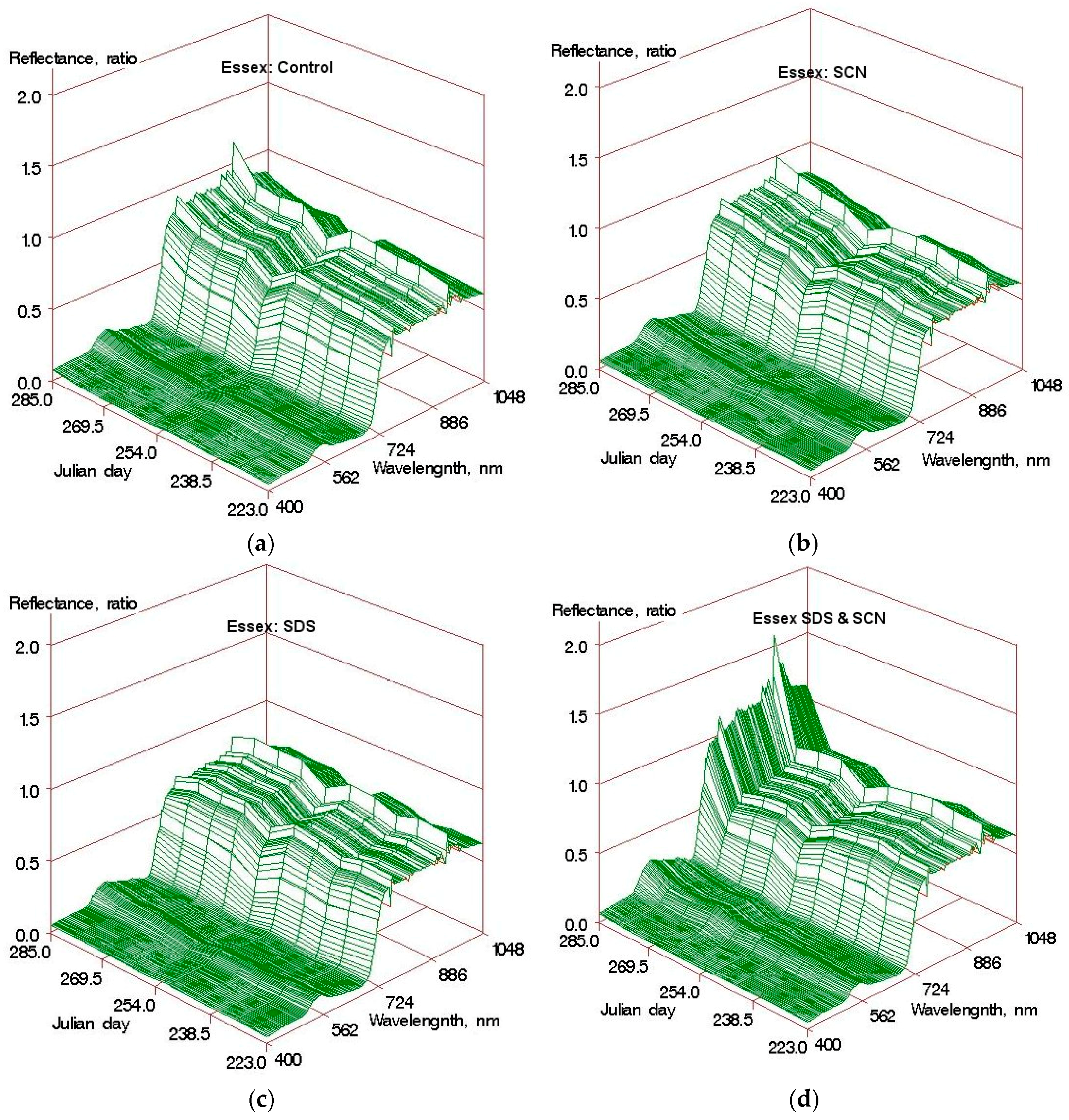
Figure 1 shows an example set of reflectance spectra illustrating how leaf reflectance of a soybean cultivar susceptible to both FV and SCN changed with plant growth under different disease treatments. The trend for healthy plants (Figure 1a) is very similar to that reported for the corn canopy by Hatfield [9], with growing green peaks from Julian day 223 to 285. As expected, SCN tended to decrease the biomass, which was indicated by a relatively slow increase or stagnation of NIR reflectance with Julian day, a measure of time, in SCN inoculated plants than in healthy plants (Figure 1). The symptoms of SCN are very similar to that of water stress since the cysts developing in the vascular tissues obstruct transport of water and nutrients. All the microplots were irrigated, providing ample water supply. Therefore, water stress-like symptoms of SCN were not visible. This is also confirmed by the reflectance spectra, which did not indicate any significant difference in the water absorption bands (950–960 nm) between SCN infected and healthy plants.
In comparison to SCN, the FV inoculated plots of Essex, the susceptible cultivar, showed drastically low NIR and high red reflectance, indicating a decrease in leaf biomass and pigment content towards the end of the data collection period. Similarly, the plants that were inoculated with both FV and SCN showed the highest reflectance in visible region, particularly in the red bands, indicating a drastic decrease in the chlorophyll content. Although the leaves used to measure the reflectance were from the top of the leaf (third or fourth from apex) and they did not show visible spotting at the early stages of FV, the difference in chlorophyll content was evident from the reflectance curves. The drastic increase in the NIR reflectance of the plants under SS treatment towards the last two dates were an artifact of data collection. Some of the plants under that treatment died completely by those dates, and, therefore, data were collected from the remaining plants in the plots that were not as severely affected, which may have caused such a trend.
3.3. Leaf Chlorophyll Content
Chlorophyll meter reading with the SPAD meter provides a measure of chlorophyll concentration in the leaf. The SPAD meter reading was used to understand how the chlorophyll concentration in leaves of plants under different disease conditions has changed. For each of the cultivars, the changes in chlorophyll index with days after planting (DAP) for the four disease treatments were compared (Figure 2). The healthy leaves of all varieties showed a nearly linear or slightly parabolic trend in chlorophyll concentration with plant growth. Chlorophyll concentration increased during the active vegetative growth, and mostly peaked out or stabilized during the reproductive stages corresponding to the latter days of data collection.
Plants infected with both FV and SCN had the most dramatic impact on chlorophyll content even when the cultivar was resistant to SDS. For example, the cultivar Pioneer showed significantly lower chlorophyll concentration in plants under SS (SDS + SCN) treatment, although it was resistant to SDS. Similarly, the cultivar Essex, which is susceptible to both diseases, showed the lowest chlorophyll concentration under SS treatment. This indicated that the presence of SDS tended to aggravate the damage caused by SCN even if the plant is resistant to SDS. Similar observations were made by many scientists on the interaction between SCN and SDS [11]. Another important observation is that the chlorophyll deterioration started earlier in SDS infected plants than SCN infected plants. For example, the chlorophyll concentration peaked out at 85 DAP in susceptible plants under SS treatment compared to 100 DAP under SDS alone, and 105 DAP under SCN alone in Essex, a cultivar susceptible to both SDS and SS. Our results agree with similar observations made by Rupe et al. [10].
3.4. Disease Correlation with Spectral Bands and Vegetation Index
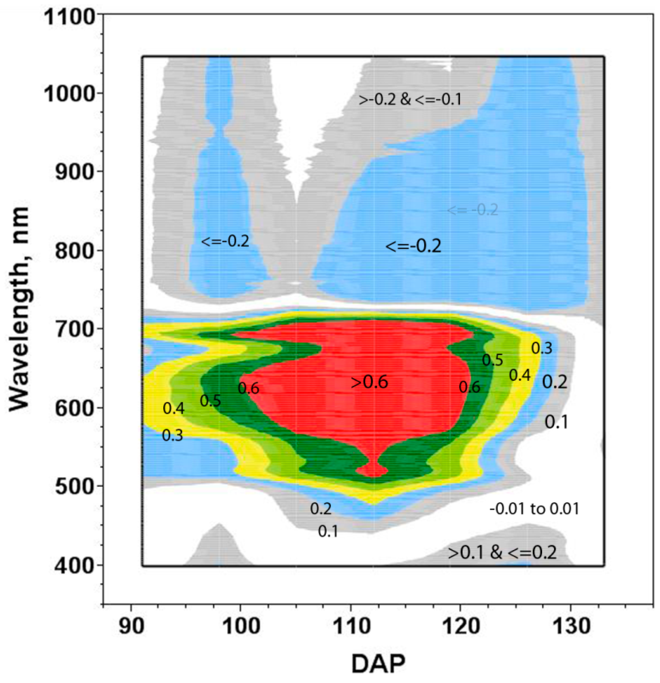
A simple correlation analysis between reflectance at individual wavebands and disease rating at different days of data collection showed that the wavelengths from 500 nm to 700 nm were more correlated to soybean disease than the NIR and blue wavebands (Figure 3). In addition, the highest correlation between disease rating and leaf reflectance occurred between 105 and 120 DAP. Before and after this window, the correlation decreased gradually. No visible disease symptoms were present until 91 DAP, and disease infestation was relatively mild until 105 DAP.
The best bands for disease discrimination identified varied with the method used. The top ten wavebands selected by the three methods (linear discriminant analysis, logistic discriminant analysis and simple correlation) included green to red edge bands in linear DA, blue, red and red edge of logistic DA and blue to red bands for simple correlation (Table 4).
The correlation between VI and disease rating varied with DAP (Table 5). The VI that showed the highest correlation to disease rating included Modified Soil Adjusted Vegetation Index-2 (MSAVI2), Normalized Difference Vegetation Index (NDVI), Photochemical Reflectance Index (PRI), Structure Independent Pigment Index (SIPI), and C420. The highest correlation with VI was observed during the three dates of 105, 112 and 119 DAP. In general, the best correlation was observed at 112 DAP except in the case of SIPI. If early detection of disease is of interest, SIPI would potentially be a good index to use. The two best VI for early detection of the disease is perhaps PRI and SIPI since they showed the highest correlation at 98 and 105 DAP. A correlation coefficient of 0.83 between SIPI and disease rating indicates that SIPI was able to explain 69% of variability in disease rating. The highest correlation coefficient obtained was −0.88 between MSAVI2 and disease rating at 112 DAP. The negative correlation indicates that the MSAVI2 decreases as disease rating increases, and MSAVI2 was able to explain 77% of variability in disease rating on that particular day. Although the disease correlation is high on individual dates, the pooled data from all dates showed poor correlation between VI and disease.
3.5. Disease Discrimination Models
If a plant showed any disease symptoms, and sustained it at some level in the following weeks, it was treated as an infested plant. Many disease ratings of 5% were not sustained during the following weeks. Therefore, a disease rating of 5% that was not sustained in the following weeks was counted as an uncertain rating, and the plants were categorized as healthy plants. A plant is also considered healthy if it did not develop any symptoms, irrespective of the disease treatment applied to the plant. The initial models for disease discrimination included the four disease levels of healthy, SCN, SDS and SS.
The linear discriminant model using the entire reflectance data showed very similar high accuracies of over 90% for identifying healthy plants under calibration data and cross-validation (Table 6). However, the accuracy for identifying various disease conditions was poor, varying from 11.5% to 18.9%. Limiting the number of inputs to 10 reflectance bands in the LDA model reduced the accuracy of identifying the healthy plants by approximately 10%, but doubled the accuracy of identifying disease conditions under cross-validation. Still, the accuracy of disease detection varied from 18% to 44.6% for the three disease conditions.
The LDA models on VI showed similar to slightly better accuracies for disease detection as the LDA model on 10 reflectance bands (Table 6). The classification accuracy for SS was slightly over 50%, considerably higher for the LDA model on 10 VIs than the reflectance based model. This is an indication that some of the VIs in the model are able to capture information relevant to the disease condition of the plant better than the raw reflectance data.
The logistic discriminant models developed using the stepwise selection procedure was able to classify 91.2% of the healthy plants when leaf reflectance was used as input, and 94% of healthy plants when VI was used as the input (Table 7). This was very similar to the performance of the linear discriminant model. The logistic discriminant models were not able to identify any of the plants with SCN while the linear discriminant model identified a few, 6.4% under calibration and 5.7% under validation. Only 24.1% of SDS plants and 17.9% of SS plants were correctly classified with logistic discriminant models on leaf reflectance, while 22.7% of SDS and 30.2% SS plants were correctly identified with the logistic discriminant model on VI. A large proportion of the infested plants were classified as healthy.
The logistic discriminant model selected a slightly different group of wavebands and VI as inputs, compared to the linear discriminant model. For example, the logistic discriminant model chose the ten best wavebands listed in Table 4 as inputs in the model based on leaf reflectance, and GRVI, C420, TVI, SIPI, MCARI, NDVI, WDRVI, RVI, NDRE and mSR as inputs in the model based on VI. The VI SIPI and mSR were inputs in the logistic discriminant model, not in the linear discriminant model.
Because of the slightly better performance of the linear discriminant model over the logistic discriminant model, the linear discriminant method was chosen for developing the modified model for classifying plants to healthy or infested. This modified model was able to classify the plants into a healthy category with 97% of accuracy under both calibration and validation, and infested plants with 68% accuracy under calibration, and 58% accuracy under validation (Table 8).
4. Discussion
Overall, the wavebands and vegetation indices that were most influential in determining disease conditions generated in this experiment varied depending on the method used to identify them. There was no consistency even in the best wavebands or the region where the bands were identified from except that all methods identified bands from the visible region. The top band identified for disease discrimination by the discriminant methods was from the red edge region (694 and 688 nm, respectively), while the correlation method identified 560 nm as the top band. Several of the top bands identified in this study or bands close to them were also identified (example, 570 nm, 700 vs. 701 nm, 690 vs. 694 nm, 730 vs. 733 nm, etc.) as critical bands by Mehlein [6] for disease identification. This study also indicated that different bands identified different diseases, as also demonstrated by Sankaran et al. [14]. Many of the VI identified in this study were also employed by other scientists for disease identification, particularly NDVI, GNDVI and MCARI [14]. Prior to 98 DAP, the correlation of disease rating with VI and leaf reflectance were very low (Figure 3 and Table 5), indicating that early detection of disease before disease symptoms are visible may be difficult. It is notable that SIPI showed the highest early correlation with disease on 98 DAP, followed by MSAVI2 and PRI (Table 5), indicating that these VIs have the best potential for detection of these diseases when symptoms are mild to moderate.
Similarly, the discriminant models were not able to identify individual diseases (SDS vs. SCN vs. SS) with high accuracy although healthy plants were identified with very high accuracy. The plants with more severe symptoms were classified more accurately while most of the error in classification occurred in plants with mild symptoms. The difficulty with disease discrimination is the lack of visible symptoms early in the season and connecting the factors causing the biophysical/chemical changes in the plants [9]. Sanakran et al. [14] indicated that the higher the visible symptoms, the better the accuracy of disease detection. Although SCN was introduced to all plants assigned for SCN treatment in this study, the water sufficient conditions (due to a wet season and irrigation) in which the plants grew minimized the stress symptoms the plant exhibited. Johnson [26] indicated that adequate soil moisture conditions maintained through irrigation caused the SCN to establish more on the root cortex instead the vascular tissues. This has limited the impact of SCN on the movement of water and nutrients through the plants, and drought-like symptoms. The natural processes are extremely complex and are influenced by a multitude of factors that may have similar impact on a plant. In addition, mild symptoms of plant diseases were difficult to identify due to the natural variability existing in the system. Mehlein [6] pointed out that the classification error reached up to 52% at low disease severity conditions.
The fact that some of the plants that were inoculated with a pathogen did not develop the disease also complicated the results. For example, there were some SDS and SCN plants that did not develop any disease for the entire season. This type of situation is typically observed in the field as well. The presence of a pathogen in the soil does not guarantee infestation or economic yield loss. A variety of factors that are related to soil, weather and plant conditions have to work together to create a favorable situation for the pathogen to succeed in infesting the plant to cause significant damage. In addition, the field data for disease was visual rating by an expert. There is inherent subjectivity and difficulty of human eyes to discriminate subtle changes repeatedly and accurately. This subjectivity may have also affected the correlation (Figure 3) and the accuracy of the discriminant models (Table 6).
Cultivar differences in canopy color, plant morphology, soil background and the diurnal variability in Sun’s position and backscattering can significantly influence the leaf and canopy reflectance spectra by introducing variability that is not related to plant health. Two vegetative indices, PRI and NDVI showed promise as potential indicators of the disease at a specific time. Since pooled data from different dates were used for model development, cultivar differences and plant biophysical changes with time had a significant effect on narrow band leaf reflectance. This may also have contributed to the modest performance of the models in identifying plants under disease conditions.
5. Conclusions
Wavebands in the green and red regions of the light spectrum showed the best correlation with disease rating as they represent pigment absorption regions, and SDS is characterized by chlorosis. The best time for disease detection seemed to be from 105 to 120 days after planting, although disease can be detected as early as 98 DAP from leaf reflectance or VI. Linear discriminant models on spectral reflectance data and VI were able to classify healthy plants with a very high accuracy of 81%–93% under cross validation, but had only modest success in identifying plants with SCN, SDS and SS. The logistic discriminant model behaved similarly, indicating that none of these discriminant models had the ability to discriminate between the three disease conditions. However, a linear discriminant model to classify between healthy and infested plants was good ability to identify the healthy plants, and modest success (58%–68% accuracy) in correctly classifying the infested plants. Disease discrimination in crop plants continues to be a challenge. Future research is required to add additional information on soil and weather to help with disease discrimination.
Acknowledgments
The authors acknowledge field support from Silvina L. Giammaria for disease assessment and rating, and the Graduate Student Research Grant from the NASA Stennis Space Center that supported Johnny Mason’s time.
Author Contributions
Sreekala Bajwa and John Rupe together planned and designed the research study. John Rupe conducted the field experiment, managed the plants throughout the season, and supervised his student in rating the plant disease. Johnny Mason, under Sreekala Bajwa’s supervision, collected the reflectance data and preprocessed the data and exported it into a spreadsheet file. Sreekala Bajwa analyzed the data and wrote this manuscript. The research was conducted at the University of Arkansas.
Conflicts of Interest
The authors declare no conflict of interest.
References
- Mahajan, G.R.; Sahoo, R.N.; Pandey, R.N.; Gupta, V.K.; Kumar, D. Using hyperspectral remote sensing techniques to monitor nitrogen, phosphorus, sulfur and potassium in wheat (Triticum aestivum L.). Precis. Agric. 2014, 15, 499–522. [Google Scholar] [CrossRef]
- Zhao, K.; Valle, D.; Popescu, S.; Zhang, X.; Mallick, B. Hyperspectral remote sensing of plant biochemistry using Bayesian model averaging with variable and band selection. Remote Sens. Environ. 2013, 132, 102–119. [Google Scholar] [CrossRef]
- Barton, C.V. Advances in remote sensing of plant stress. Plant Soil 2012, 354, 41–44. [Google Scholar] [CrossRef]
- Gebbers, R.; Adamchuk, V.I. Precision agriculture and food security. Science 2010, 327, 828–831. [Google Scholar] [CrossRef] [PubMed]
- Mulla, D.J. Twenty five years of remote sensing in precision agriculture: Key advances and remaining knowledge gaps. Biosyst. Eng. 2013, 114, 358–371. [Google Scholar] [CrossRef]
- Mahlein, A.K.; Rumpf, T.; Welke, P.; Dehne, H.W.; Plümer, L.; Steiner, U.; Oerke, E.C. Development of spectral indices for detecting and identifying plant diseases. Remote Sens. Environ. 2013, 128, 21–30. [Google Scholar] [CrossRef]
- Martinelli, F.; Scalenghe, R.; Davino, S.; Panno, S.; Scuderi, G.; Ruisi, P.; Villa, P.; Stroppiana, D.; Boschetti, M.; Goulart, L.R.; et al. Advanced methods of plant disease detection. A review. Agron. Sustain. Dev. 2015, 35, 1–25. [Google Scholar] [CrossRef]
- Mahlein, A.K.; Oerke, E.C.; Steiner, U.; Dehne, H.W. Recent advances in sensing plant diseases for precision crop protection. Eur. J. Plant Pathol. 2012, 133, 197–209. [Google Scholar] [CrossRef]
- Hatfield, J.L.; Gitelson, A.A.; Schepers, J.S.; Walthall, C.L. Application of spectral remote sensing to agronomic decisions. Agron. J. 2008, 100, S-117. [Google Scholar] [CrossRef]
- Rupe, J.; Sabbe, W.E.; Robbins, R.T.; Gbur, E.E., Jr. Soil and plant factors associated with sudden death syndrome of soybean. J. Prod. Agric. 1993, 6, 218–221. [Google Scholar] [CrossRef]
- Rupe, J.C.; Gbur, E.E., Jr. Effect of plant age, maturity group and the environment on disease progress of sudden death syndrome of soybean. Plant Dis. 1995, 79, 139–143. [Google Scholar] [CrossRef]
- Gao, X.; Jackson, T.A.; Hartman, G.L.; Niblack, T.L. Interactions between the Soybean Cyst Nematode and Fusarium solani f. sp. Glycines based on greenhouse factorial experiments. Phytopathology 2006, 96, 1409–1415. [Google Scholar] [PubMed]
- Blevins, D.G.; Dropkin, V.H.; Luedders, V.D. Macronutrient uptake, translocation, and tissue concentration of soybeans infested with the soybean cyst nematode and elemental composition of cysts isolated from roots. J. Plant Nutr. 1995, 18, 579–591. [Google Scholar] [CrossRef]
- Sankaran, S.; Mishra, A.; Ehsani, R.; Davis, C. A review of advanced techniques for detecting plant diseases. Comput. Electron. Agric. 2010. [Google Scholar] [CrossRef]
- West, J.S.; Bravo, C.; Oberti, R.; Lemaire, D.; Moshou, D.; McCartney, H.A. The potential of optical canopy measurement for targeted control of field crop diseases. Annu. Rev. Phytopathol. 2003, 41, 593–614. [Google Scholar] [CrossRef] [PubMed]
- Oerke, E.-C.; Fröhling, P.; Steiner, U. Thermographic assessment of scab disease on apple leaves. Precis. Agric. 2011, 12, 699–715. [Google Scholar] [CrossRef]
- Bock, C.H.; Poole, G.H.; Parker, P.E.; Gottwald, T.R. Plant disease severity estimated visually, by digital photography and image analysis, and by hyperspectral imaging. Crit. Rev. Plant Sci. 2010, 29, 59–107. [Google Scholar] [CrossRef]
- Bürling, K.; Hunsche, M.; Noga, G. Use of blue-green and chlorophyll fluorescence measurements for differentiation between nitrogen deficiency and pathogen infection in wheat. J. Plant Physiol. 2011, 168, 1641–1648. [Google Scholar] [CrossRef] [PubMed]
- Stoll, M.; Schultz, H.R.; Baecker, G.; Berkelmann-Loehnertz, B. Early pathogen detection under different water status and the assessment of spray application in vineyards through the use of thermal imagery. Precis. Agric. 2008, 9, 407–417. [Google Scholar] [CrossRef]
- Oerke, E.-C.; Steiner, U.; Dehne, H.-W.; Lindenthal, M. Thermal imaging of cucumber leaves affected by downy mildew and environmental conditions. J. Exp. Bot. 2006, 57, 2121–2132. [Google Scholar] [CrossRef] [PubMed]
- Calderón, R.; Navas-Cortés, J.A.; Lucena, C.; Zarco-Tejada, P.J. High-resolution airborne hyperspectral and thermal imagery for early detection of Verticillium wilt of olive using fluorescence, temperature and narrow-band spectral indices. Remote Sens. Environ. 2013, 139, 231–245. [Google Scholar] [CrossRef]
- Hillnhütter, C.; Mahlein, A.-K.; Sikora, R. A.; Oerke, E.-C. Remote sensing to detect plant stress induced by Heterodera schachtii and Rhizoctonia solani in sugar beet fields. Field Crop. Res. 2011, 122, 70–77. [Google Scholar] [CrossRef]
- Mahlein, A.-K.; Steiner, U.; Dehne, H.-W.; Oerke, E.-C. Spectral signatures of sugar beet leaves for the detection and differentiation of diseases. Precis. Agric. 2010, 11, 413–431. [Google Scholar] [CrossRef]
- Bajwa, S.G.; Bajcsy, P.; Groves, P.; Tian, L.F. Hyperspectral image data mining for band selection in agricultural applications. Trans. ASAE 2004, 47, 895–907. [Google Scholar] [CrossRef]
- Nutter, F.W., Jr.; Tylka, G.L.; Guan, J.; Moreira, A.J.D.; Marett, C.C.; Rosburg, T.R.; Basart, J.P.; Chong, C.S. Use of remote sensing to detect soybean cyst nematode-induced plant stress. J. Nematol. 2002, 34, 222–231. [Google Scholar] [PubMed]
- Johnson, A.B.; Kim, K.S.; Riggs, R.D.; Scott, H.D. Location of Heterodera glycines-induced syncytia in soybean as affected by soil water regimes. J. Nematol. 1993, 25, 422–426. [Google Scholar] [PubMed]
Figure 1.
Temporal variation in the visible-near-infrared (VNIR) reflectance of a soybean leaf for cultivar Essex under four disease treatments (a) through (d). Essex is susceptible to both soybean cyst nematode (SCN) and sudden death syndrome (SDS). (a) Un-inoculated (UN) or control; (b) Soybean inoculated with SCN; (c) Soybean inoculated with SDS; (d) Soybean inoculated with SCN and SDS (SS).

Figure 2.
Change in chlorophyll content, measured with a chlorophyll meter, plotted against time in four soybean cultivars under four disease treatments, namely, Control (UN), soybean cyst nematode (SCN), sudden death syndrome (SDS), and SCN + SDS (SS). The four cultivars were Asgrow 5603 (A-SDS susceptible), Essex (E-SDS & SCN susceptible), Hartwig (H-SDS & SCN resistant) and Pioneer (P-SCN susceptible).
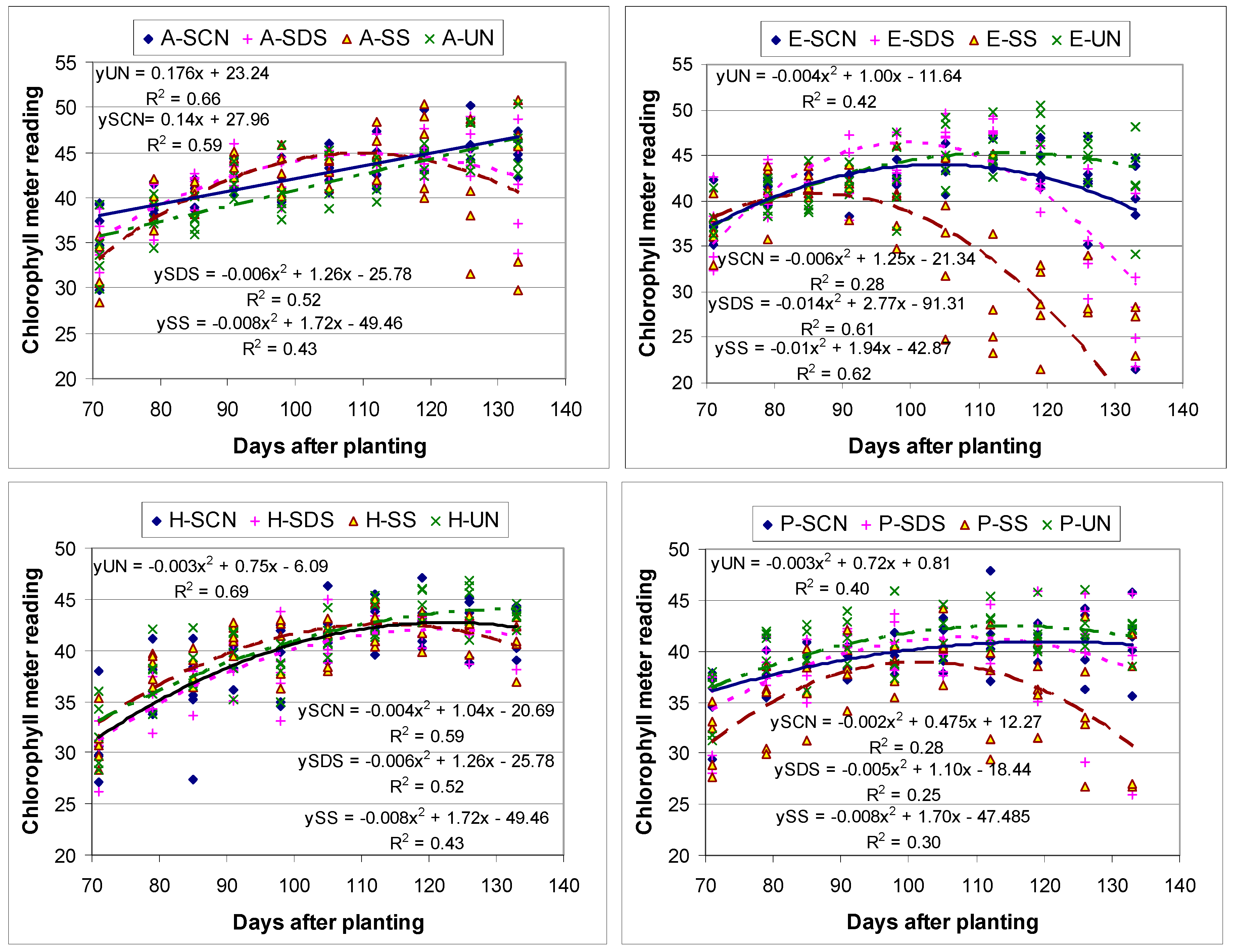
Figure 3.
A contour plot of linear correlation between leaf reflectance at different wavelengths and disease rating as a function of days after planting (DAP).
Figure 3.
A contour plot of linear correlation between leaf reflectance at different wavelengths and disease rating as a function of days after planting (DAP).


Table 1.
Details of experimental design used in the field study with four cultivars and four disease treatments. The four disease treatment included combinations of two pathogens, sudden death syndrome (SDS) caused by F. virguliforme (FV) and soybean cyst nematode (SCN) caused by H. glycines (HG), both (SS), or neither (Control or healthy). All treatment combinations were replicated five times.
| Experiment Variable | Treatment Levels | Treatment Traits |
|---|---|---|
| Cultivar | Pioneer 9594 | SDS resistant, SCN susceptible |
| Asgrow 5603 | SDS susceptible, SCN resistant | |
| Hartwig | SDS resistant, SCN resistant | |
| Essex | SDS susceptible, SCN susceptible | |
| Disease | Control | No disease (healthy) |
| FV inoculated | Sudden death syndrome (SDS) | |
| HG inoculated | Soybean Cyst Nematode (SCN) | |
| FV and HG co-inoculated | SDS and SCN (SS) |
| VI | Description | Formulation |
|---|---|---|
| C420 | C420 | |
| NDVI | Normalized Difference Vegetation Index | |
| GNDVI or GRVI | Green Normalized Difference Vegetation Index | |
| MSAVI2 | Modified SAVI-2 | |
| PRI | Photochemical Reflectance Index | |
| mSR | Modified Spectral Ratio | |
| REIP | Red Edge Inflection Point | |
| WDRVI | Wide Dynamic Range Vegetation Index | |
| SIPI | Structure Independent Pigment Index | |
| TVI | Triangular Vegetation Index | |
| NDRE | Normalized Difference Red Edge Index | |
| RVI | Ratio Vegetation Index | |
| MCARI | Modified Chlorophyll Absorption in Reflectance Index |
Table 3.
Disease infestation statistics for different cultivars under the 4 disease treatments of control (no disease), sudden death syndrome (SDS), soybean cyst nematode (SCN), and SCN + SDS (SS). Each cultivar × disease combination had 5 observations. Values in parentheses indicate percentage of infested plots in the specific category.
| Cultivar | Disease | Average Disease Rating and (% Frequency) at Different Days after Planting (DAP) | ||||||
|---|---|---|---|---|---|---|---|---|
| 91DAP | 98DAP | 105DAP | 112DAP | 119DAP | 126DAP | 133DAP | ||
| Pioneer 9594 | control | 0 | 0 | 0 | 0 | 0 | 7 (40) | 26 (60) |
| SCN | 0 | 0 | 0 | 0 | 1 (40) | 3 (20) | 20 (20) | |
| SDS | 0 | 0 | 0 | 1 | 5 (60) | 46 (80) | 40 (40) | |
| SS | 2 (40) | 2 (40) | 11 (80) | 16 (80) | 28 (100) | 50 (80) | 9 (20) | |
| Asgrow 5603 | control | 0 | 0 | 0 | 0 | 0 | 34 (100) | 55 (80) |
| SCN | 0 | 0 | 0 | 0 | 6.2 (20) | 30 (60) | ||
| SDS | 0 | 0 | 0 | 0 | 0 | 21 (40) | 24 (60) | |
| SS | 0 | 0 | 0 | 0 | 2 (100) | 4 (60) | 4 (60) | |
| Hartwig | control | 0 | 0 | 0 | 0 | 0 | 0 | 0 |
| SCN | 0 | 0 | 0 | 0 | 0 | 0 | 0 | |
| SDS | 0 | 0 | 0 | 0 | 0 | 2 (40) | 6 (80) | |
| SS | 0 | 0 | 0 | 0 | 0 | 4 (40) | 17 (20) | |
| Essex | control | 0 | 0 | 0 | 0 | 0 | 14 (40) | 18 (20) |
| SCN | 0 | 0 | 0 | 0 | 1 (60) | 12 (80) | 16 (60) | |
| SDS | 0 | 0 | 1 | 1 (40) | 7 (100) | 6 (40) | 13 (60) | |
| SS | 30 (100) | 30 (100) | 34 (100) | 51 (100) | 73 (100) | 61 (100) | 63 (100) | |
Table 4.
The ten best wavebands for disease discrimination, selected through three different methods namely linear discriminant analysis (DA), logistic discriminant analysis, and linear correlation analysis on the pooled data.
| Band Rank | Linear DA | Logistic DA | Correlation |
|---|---|---|---|
| 1 | 694 | 688 | 560 |
| 2 | 535 | 703 | 461 |
| 3 | 766 | 421 | 458 |
| 4 | 733 | 400 | 494 |
| 5 | 658 | 427 | 485 |
| 6 | 523 | 682 | 479 |
| 7 | 1015 | 571 | 632 |
| 8 | 700 | 679 | 686 |
| 9 | 931 | 559 | 626 |
| 10 | 592 | 589 | 476 |
Table 5.
Correlation between disease rating and vegetation indices, starting at Julian day 243, which is also 91 days after planting (DAP). Prior to this date, no disease symptoms were observed on plants. The highest five significant correlations are highlighted with bold and italics.
| VI | 91 DAP | 98 DAP | 105 DAP | 112 DAP | 119 DAP | 126 DAP | 133 DAP |
|---|---|---|---|---|---|---|---|
| C420 | −0.30 | −0.68 | −0.75 | −0.86 | −0.77 | −0.35 | 0.14 |
| NDVI | −0.40 | −0.71 | −0.78 | −0.87 | −0.77 | −0.40 | −0.16 |
| GNDVI | −0.29 | −0.50 | −0.63 | −0.77 | −0.63 | −0.27 | −0.19 |
| GRVI | 0.12 | 0.42 | 0.42 | 0.67 | 0.49 | 0.41 | 0.11 |
| MSAVI2 | −0.36 | −0.74 | −0.72 | −0.88 | −0.78 | −0.42 | −0.13 |
| PRI | 0.33 | 0.74 | 0.80 | 0.81 | 0.77 | 0.36 | −0.11 |
| mSR | −0.30 | −0.47 | −0.63 | −0.74 | −0.66 | −0.31 | −0.14 |
| REIP | −0.33 | −0.61 | −0.53 | −0.79 | −0.67 | −0.32 | −0.16 |
| WDRVI | −0.33 | −0.69 | −0.75 | −0.85 | −0.73 | −0.39 | −0.17 |
| SIPI | 0.25 | 0.83 | 0.83 | 0.80 | 0.69 | 0.42 | 0.21 |
| TVI | −0.37 | −0.63 | −0.60 | −0.78 | −0.67 | −0.13 | 0.07 |
| NDRE | −0.31 | −0.47 | −0.56 | −0.73 | −0.66 | −0.28 | −0.07 |
| RVI | −0.29 | −0.60 | −0.67 | −0.77 | −0.68 | −0.33 | −0.15 |
| MCARI | 0.29 | 0.41 | 0.64 | 0.57 | 0.60 | 0.02 | −0.09 |
Table 6.
Classification accuracy with Linear Discriminant Analysis (LDS) performed on reflectance data with all bands and 10 best bands identified in Table 4 as well as all vegetation indices (VI) and the 10 best VI.
| Class | % Accuracy under Calibration | % Accuracy under Cross-Validation | ||||||
|---|---|---|---|---|---|---|---|---|
| Healthy | SCN | SDS | SS | Healthy | SCN | SDS | SS | |
| LDA Model with all Spectral Bands | ||||||||
| Healthy | 95.6 | 0.5 | 1.1 | 0.5 | 93.3 | 1.4 | 4.4 | 0.5 |
| SCN | 52.5 | 18.9 | 5.7 | 0.8 | 77.9 | 11.5 | 2.4 | 2.5 |
| SDS | 41.7 | 2.3 | 25.7 | 4.0 | 70.9 | 1.7 | 18.9 | 4.0 |
| SS | 53.0 | 0.0 | 4.6 | 24.4 | 69.7 | 1.5 | 9.1 | 12.1 |
| LDA Model with all 10 selected bands | ||||||||
| Healthy | 85.5 | 1.1 | 3.5 | 0.5 | 82.7 | 3.7 | 11.1 | 2.1 |
| SCN | 44.3 | 22.1 | 8.2 | 3.3 | 63.1 | 18.0 | 10.6 | 2.5 |
| SDS | 26.3 | 5.7 | 46.6 | 0.6 | 44.5 | 5.7 | 44.6 | 2.3 |
| SS | 27.3 | 6.1 | 10.6 | 37.9 | 34.9 | 7.6 | 15.1 | 30.3 |
| LDA Model on all VIs | ||||||||
| Healthy | 89.0 | 2.6 | 3.1 | 0.7 | 84.5 | 7.2 | 6.6 | 1.3 |
| SCN | 39.0 | 32.6 | 2.8 | 2.8 | 55.3 | 32.6 | 4.3 | 4.3 |
| SDS | 32.2 | 4.7 | 32.9 | 1.3 | 53.0 | 5.4 | 32.2 | 3.4 |
| SS | 20.8 | 6.2 | 10.4 | 43.8 | 37.5 | 8.3 | 14.6 | 33.3 |
| LDA Model on top VIs (GRVI, RVI, MCARI, NDRE, RVI, C420, NDVI, GNVDI, WDRVI) | ||||||||
| Healthy | 87.7 | 2.1 | 4.8 | 0.9 | 81.6 | 6.7 | 9.4 | 1.1 |
| SCN | 27.8 | 28.6 | 8.7 | 4.0 | 53.1 | 26.2 | 11.9 | 3.2 |
| SDS | 23.8 | 4.6 | 46.5 | 2.9 | 44.2 | 5.8 | 42.4 | 3.5 |
| SS | 20.6 | 1.6 | 11.1 | 57.1 | 27.0 | 1.6 | 17.5 | 52.4 |
Table 7.
Classification accuracy with Logistic Discriminant Model (n = 799) developed on leaf reflectance data as well as vegetation index data using the ten best input variables. The model on VI chose GRVI, C420, TVI, SIPI, MCARI, NDVI, WDRVI, RVI, NDRE and mSR as the best input variables.
| Class | % Accuracy for Reflectance Model | % Accuracy for VI Model | ||||||
|---|---|---|---|---|---|---|---|---|
| Healthy | SCN | SDS | SS | Healthy | SCN | SDS | SS | |
| Healthy | 91.2 | 0.0 | 8.1 | 0.5 | 94.0 | 0.0 | 6.0 | 0.0 |
| SCN | 82.8 | 0.0 | 15.6 | 1.6 | 89.7 | 0.0 | 7.9 | 2.4 |
| SDS | 72.4 | 0.0 | 24.1 | 2.9 | 72.7 | 0.0 | 22.7 | 4.7 |
| SS | 47.8 | 0.0 | 32.8 | 17.9 | 44.4 | 0.0 | 25.4 | 30.2 |
Table 8.
Result of plant classification using the linear and logistic discriminant analysis for n = 799.
| Classification Category | Linear Discriminant Analysis | Validation | ||
|---|---|---|---|---|
| Healthy (%) | Infested (%) | Healthy (%) | Infested (%) | |
| Healthy | 97 | 3 | 97 | 3 |
| Infested | 32 | 68 | 42 | 58 |
© 2017 by the authors. Licensee MDPI, Basel, Switzerland. This article is an open access article distributed under the terms and conditions of the Creative Commons Attribution (CC BY) license ( http://creativecommons.org/licenses/by/4.0/).
Share and Cite
MDPI and ACS Style
Bajwa, S.G.; Rupe, J.C.; Mason, J. Soybean Disease Monitoring with Leaf Reflectance. Remote Sens. 2017, 9, 127. https://doi.org/10.3390/rs9020127
AMA Style
Bajwa SG, Rupe JC, Mason J. Soybean Disease Monitoring with Leaf Reflectance. Remote Sensing. 2017; 9(2):127. https://doi.org/10.3390/rs9020127
Chicago/Turabian StyleBajwa, Sreekala G., John C. Rupe, and Johnny Mason. 2017. "Soybean Disease Monitoring with Leaf Reflectance" Remote Sensing 9, no. 2: 127. https://doi.org/10.3390/rs9020127
Note that from the first issue of 2016, this journal uses article numbers instead of page numbers. See further details here.