Combining Partial Least Squares and the Gradient-Boosting Method for Soil Property Retrieval Using Visible Near-Infrared Shortwave Infrared Spectra

Abstract

Soil spectroscopy has experienced a tremendous increase in soil property characterisation, and can be used not only in the laboratory but also from the space (imaging spectroscopy). Partial least squares (PLS) regression is one of the most common approaches for the calibration of soil properties using soil spectra. Besides functioning as a calibration method, PLS can also be used as a dimension reduction tool, which has scarcely been studied in soil spectroscopy. PLS components retained from high-dimensional spectral data can further be explored with the gradient-boosted decision tree (GBDT) method. Three soil sample categories were extracted from the Land Use/Land Cover Area Frame Survey (LUCAS) soil library according to the type of land cover (woodland, grassland, and cropland). First, PLS regression and GBDT were separately applied to build the spectroscopic models for soil organic carbon (OC), total nitrogen content (N), and clay for each soil category. Then, PLS-derived components were used as input variables for the GBDT model. The results demonstrate that the combined PLS-GBDT approach has better performance than PLS or GBDT alone. The relative important variables for soil property estimation revealed by the proposed method demonstrated that the PLS method is a useful dimension reduction tool for soil spectra to retain target-related information.

1. Introduction

Monitoring the status of soil is very important for tackling many challenges including food security, climate change, land degradation, and biodiversity [1]. Traditional laboratory technologies to analyse soil are often time consuming and expensive, and these soil analyses are usually limited to a few samples and lack information on the spatial variability of soil [2]. Soil spectroscopy, as a fast, cost-effective, and environmental-friendly analytical technique, has successfully been utilised to retrieve soil properties and has experienced a tremendous increase in the past years. It has been shown that soil spectra across the Visible Near-Infrared Shortwave Infrared (VIS–NIR–SWIR; 400–2500 nm) spectral region are characterised by significant spectral signals [3,4,5,6], which makes it possible for quantitative analysis of soil properties. Furthermore, the wide spread use of visible and infrared spectroscopy can resolve the trade-off between the growing need of large scale soil information and its high cost [7]. Using spectral measurements and corresponding soil properties measured by soil analyses, soil spectroscopy can be adopted to quantitatively estimate many soil properties, such as organic matter, heavy metals, clay content, exchangeable potassium, and electrical conductivity [8,9,10].

The multivariate analysis technique is vital for quantitative analysis of soils. Partial least squares (PLS) regression is frequently used for spectroscopic data and demonstrates good capability for the estimation of soil properties. The PLS regression method can relate the response variable with relevant information from the spectra while keeping fewer PLS components or factors. It has been successfully demonstrated that the use of soil spectroscopy and PLS regression can quantify soil properties, and an automatic modelling engine PARACUDA^®, including PLS, was developed to predict various soil properties using reflectance data [11,12]. PARACUDA^® is proposed based on the all-possibilities-approach (APA) concept and uses a covariate optimisation routine to select the best pre-processing steps (1st and 2nd derivatives, continuum removal (CR), standard normal variate (SNV), etc.) [13]. Besides PARACUDA^®, various calibration methods were also developed based on PLS. The autoPLSR method was proposed to save the need for manual fine-tuning and provides a non-expert, automatic, feature, and latent variable selection, and it was successfully applied for soil clay and iron quantitative mapping using airborne hyperspectral data [14]. The focus of PLS regression is to find the relevant linear subspace of the latent variables, and it has not implemented of variable selection, which could be done based on the selectivity ratio or variable importance for the projection (VIP) before developing PLS models [15,16,17]. Another option is to use interval PLS (iPLS), which selects only the important variable intervals for PLS regression [18]. Besides, a genetic algorithm was combined with PLS regression (GA-PLSR) to select the most informative spectral variables and thus to improve the prediction accuracies compared with support vector machine regression (SVMR) [9,19]. A memory-based learning (MBL) method called locally weighted partial least squares regression (LWR) was also developed and compared with multiple linear regression (MLR), multiple regression after principal components compression (MLRPC), and PLS. The highest prediction accuracies for most of the soil attributes evaluated were produced by LWR [20]. PLS regression often has performs better on a local scale. Therefore, several different local PLS modelling approaches were proposed and evaluated for predicting soil attributes using a large soil spectral library across the French territory [21]. MBL is a data-driven approach. It is very flexible and can be easily combined with other approaches. MBL describes the target function as a collection of less complex local stable approximations [22,23]. However, it is pointed out that memory-based methods have drawbacks such as high computational costs, and the similarity measure used for recovering samples from the nearest neighbours fails to fit a global function. A spectrum-based learner (SBL) was proposed based on MBL, which can be described as a local linear Gaussian processing modelling approach combining local distance matrices and spectral features as a source of input variables. SBL is able to produce reliable models using regional and global soil spectral libraries [22].

PLS can also be utilised as a dimension reduction (DR) tool [24,25,26,27], which has scarcely been explored in soil spectroscopy. The underlying assumption of PLS is that the observed data is generated by a process that is driven by a small number of latent (not directly observed or measured) variables [28]. The reason why PLS regression can perform better than other well-known regression techniques, such as multiple linear regression and ridge regression, is the stability of components derived from the PLS method [29]. The new components can be viewed as retained variables and act as inputs for many other regression approaches. Gradient-boosted decision trees (GBDT), also known as gradient-boosting machine (GBM) or multiple additive regression trees (MART), are one of the most widely used machine learning algorithms and can be viewed as a gradient-boosting algorithm using the decision tree as the weak learner [30,31]. The GBDT method is an additive classification or regression model consisting of an ensemble of trees. It is highly adaptable and many different loss functions can be used during boosting. However, building an accurate GBDT model is time-consuming and often requires extensive parameter tuning. Hence, A GPU-based approach was proposed to accelerate the speed [32].

The relationship between soil properties and soil spectra is very complicated and has an inherently non-linear nature. The objective of the study is to explore the potential of PLS as a dimension reduction tool for soil spectra and the performance of GBDT on the estimation of soil properties. A European-scale soil spectral library has been developed in the framework of Land Use/Land Cover Area Frame Survey (LUCAS) and contains ~20,000 geo-referenced top-soil samples, which is an ideal dataset to evaluate the performance of the proposed PLS-GBDT method. Three categories of soil samples were extracted from the LUCAS soil spectral library according to the type of land cover (woodland, cropland, and grassland). For each category, organic carbon (OC), clay, and total nitrogen content (N) were modelled with the proposed method. The evaluation of variable importance was performed and compared with results obtained from PLS and GBDT models.

2. Materials and Methods

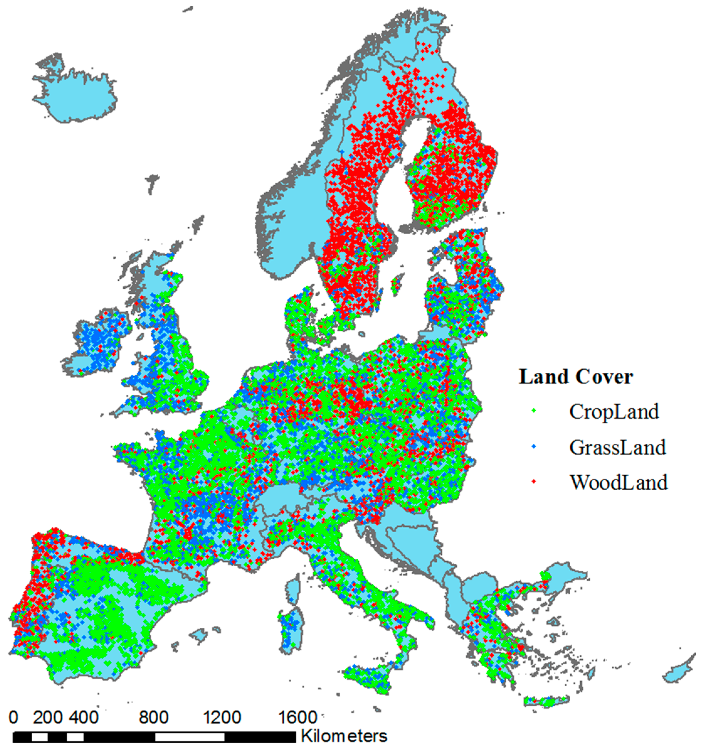
2.1. The LUCAS Soil Spectral Library

As part of the LUCAS project, approximately 20,000 geo-referenced topsoil samples were collected and analysed in the 25 European Union Member States [33,34]. This is the first attempt to build a consistent soil database, which provides an excellent basis to assess topsoil characteristics across the European Union. A standardised sampling procedure was used to collect around 0.5 kg of topsoil (0–20 cm). The collected soils were sampled from different land covers and can be classified as mineral and organic soils. In this paper, the proposed method was applied to mineral soil samples from woodland, cropland, and grassland, the distribution of which can be seen in Figure 1.

The Vis-NIR soil spectra were measured using a FOSS XDS Rapid Content Analyser (FOSS NIRSystems Inc., Hilleroed, Denmark), operating in the 400–2500 nm wavelength range, with 0.5 nm spectral resolution. Pre-processing included removal of the data at wavelengths of 400–500 nm that showed instrumental artefacts, transformation of absorbance (A) spectra into reflectance (1/10^A) spectra, continuum removal, Savitzky-Golay Filter with a window size of 51 and 2nd order polynomial, and resampling to contain 200 bands. 13 soil properties were analysed in a central laboratory. Three key soil properties, soil organic carbon (OC), total nitrogen content (N), and clay, were selected as our studied properties. A brief statistical summary of soil properties is listed in

Table 1. Summary statistics of soil properties (organic carbon (OC), total nitrogen content (N), and clay) for the three soil categories.

Category	Property	N	Mean	SD	Min	Q25	Q50	Q75	Max
Woodland	OC (g/kg)	4182	37.3	24.1	0.0	18.8	31.4	50.8	125.8
	N (g/kg)	4182	2.0	1.3	0.0	1.0	1.7	2.6	9.1
	Clay (%)	4182	11.3	10.4	0.0	4.0	7.0	16.0	65.0
Cropland	OC (g/kg)	8341	17.1	10.9	0.0	10.4	14.4	20.5	160.3
	N (g/kg)	8341	1.6	0.79	0.0	1.1	1.5	1.9	9.5
	Clay (%)	8341	22.1	12.7	1.0	13.0	21.0	30.0	79.0
Grassland	OC (g/kg)	3957	30.2	19.0	0.0	15.7	25.9	39.2	165.7
	N (g/kg)	3957	2.7	1.5	0.0	1.5	2.3	3.4	13.6
	Clay (%)	3957	19.9	12.4	0.0	11.0	18.0	27.0	79.0

SD: Standard Deviation; Q25: lower quartile; Q50: median; Q75: upper quartile.

.

2.2. Partial Least Squares Algorithm

PLS regression has proven to be a very successful method for multivariate data analysis. It is a standard tool in chemometrics and has received a great amount of attention in the field of soil spectroscopy. It is similar to principal component regression (PCR), as both can overcome the problems of high dimensionality and multicollinearity. In its classical form, the PLS method is based on the nonlinear iterative partial least squares (NIPALS) algorithm. To calibrate a PLS regression model for each soil property, the optimal number of latent variables was identified by performing a 10-fold cross validation, and the root-mean-square error (RMSE) in the cross-validation was used as decision criterion. Besides directly applying PLS regression to soil spectra, the transformed PLS components were also used as inputs for the following gradient-boosting model.

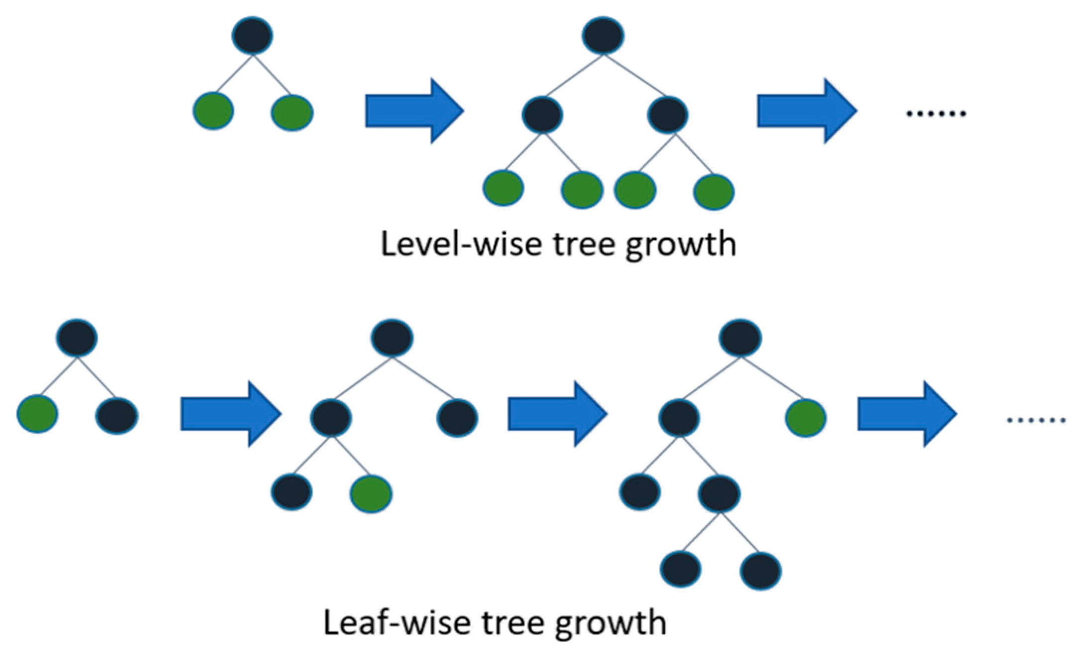
2.3. Gradient-Boosted Decision Trees (GBDT)

Gradient-boosting is a machine learning technique for regression and classification problems, which was developed by Jerome Friedman [35,36]. One of the widely used gradient-boosting methods is GBDT, which is highly adaptable and able to model feature interactions and inherently perform feature selection [37]. These features have made GBDT one of the most widely used machine learning algorithms. Gradient-boosting develops an ensemble of tree-based models by training each of the trees in a sequential manner. Each iteration fits a decision to the residuals left by the previous one and then prediction is accomplished by combining the trees. It can produce robust and interpretable procedures for both regression and classification. Mathematically, the model can be viewed as:

$${\widehat{y}}_i={\displaystyle \sum }_{k=1}^K{f}_k\left(x_i\right),f_k\in F$$

(1)

where $k$ is the number of trees, $f$ is a function in the functional space $F$, and $F$ is the set of all possible regression trees.

There are several open-source projects that have implemented GBDT, like scikit-learn, XGBoost, and LightGBM [30,38,39]. LightGBM [40] is used in this study, and it is developed by Microsoft. It takes advantage of histogram-based algorithms to accelerate training process and reduce memory consumption by aggregating continuous features into discrete bins [41]. Most decision tree learning algorithms grow trees by level-wise or depth-wise approach, as shown in Figure 2; LightGBM grows trees by leaf-wise or best-first approach. It will choose the leaf with max delta loss to grow. When growing the same number of leafs, leaf-wise algorithm can reduce more loss than level-wise algorithm. LightGBM also supports parallel and GPU learning, and it is capable of handling large-scale data.

Soil spectra quantitatively correlates with soil properties. By fitting a regression model, it is supposed to achieve a good predictive accuracy for the estimation of soil property. There are many parameters that need to be tuned in GBDT, like learning rate or shrinkage, max depth, number of trees, etc. Reducing the learning rate parameter helps prevent overfitting and has a smoothing effect but increases the learning time [31]. The learning rate was set to 0.05. Parameters of max depth and number of trees can also determine whether the model is over fitted or not, and these two parameters were explored using a grid search strategy.

2.4. Calculation of Relative Variable Importance

PLS regression and the gradient-boosting method both can estimate relative contribution of each input variable or feature. The resultant variable importance measure is useful for understanding the relevance of contributing wavelengths. Ranking based on relative contribution values can help to identify the reflectance bands that are most important for developing soil spectroscopic models. In general, the top few bands contribute most for the model development. For PLS algorithm, the calculation of important input variables are based on weighted sums of the absolute PLS-regression coefficients. A large loading also indicates the importance of a variable. Here, we use the VIP score derived from coefficients to assess the importance of input variables. It calculates the contribution of independent variables to the contribution of the dependent variable. For the gradient-boosting method, the importance of input variable can be calculated based on metric of “split” or “gain”. “Split” is the number of times a variable is used in a model and “gain” is the total gain of splits that use the variable. We use split as the descriptor of relative variable importance in this study. The more a variable is used to make key decisions with decision trees, the higher its relative importance.

2.5. Assessment

For each soil property, the soil spectral quantitative model was developed on a random sample of two-thirds of the selected soil samples using PLS regression or the gradient-boosting regression method. The calibrations were tested by predicting the soil properties on validation dataset composed of the remaining one-third samples for each soil category. The model accuracies were evaluated on estimated and measured soil OC, N, and clay values using coefficient of determination (R²), RMSE, and the ratio of performance to deviation (RPD) [42].

$$R^2=\frac{{{\displaystyle \sum }}_{i=1}^n{\left({\widehat{y}}_i-\overline{y}\right)}^2}{{{\displaystyle \sum }}_{i=1}^n{\left(y_i-\overline{y}\right)}^2}$$

(2)

$$RMSE=\sqrt{\frac{1}{n}{{\displaystyle \sum }}_{i=1}^n{\left({\widehat{y}}_i-y_i\right)}^2}$$

(3)

$$RPD=\frac{SD}{RMSE}$$

(4)

where n is the number of validation samples, $y$ is the measured value, $\overline{y}$ is the mean of the measured value, and $\widehat{y}$ is the estimated value.

3. Results

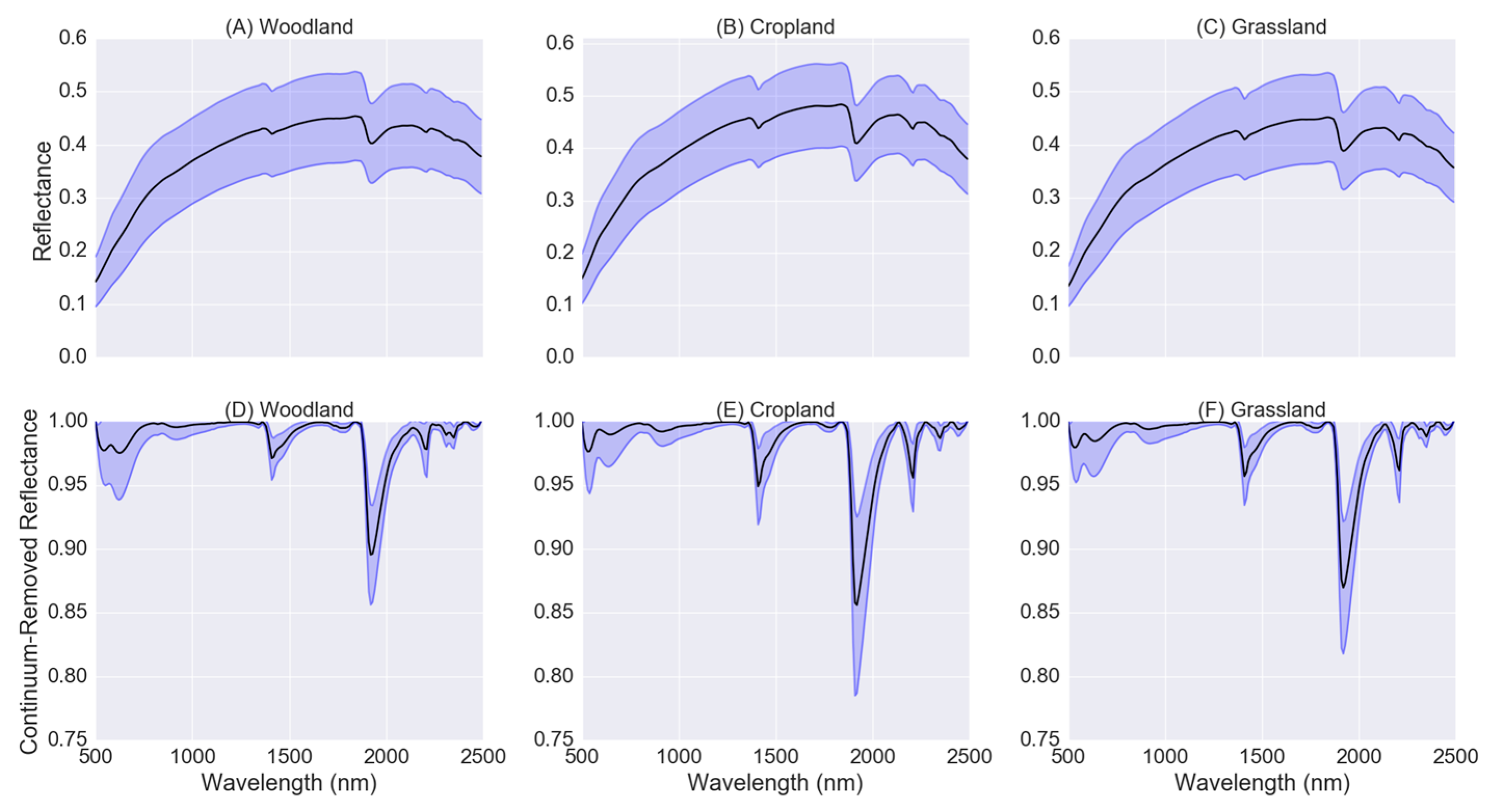
3.1. Overview of the Spectral Measurement of Soil Samples

The mean soil reflectance spectra and standard deviations for soil samples from woodland, cropland, and grassland were plotted in Figure 3. The mean spectra of three soil categories have a similar curve shape whose reflectance values increase with increasing wavelength in the range of 500–1300 nm. Absorption features can be identified near 1400 and 1900 nm, which are assigned to soil hygroscopic water in clay minerals [43]. The mean soil CR spectra and standard deviations for samples from woodland, cropland, and grassland are also shown. CR spectra can be used to isolate and identify characteristic absorptions of minerals, organic compounds, and water in soils [3]. The main spectral difference is that the mean reflectance spectrum for cropland soils demonstrates a higher albedo than spectra for woodland and cropland soils, as cropland soils have a lower mean value of OC content (17.1 g/kg) than woodland soils (37.3 g/kg) and grassland soils (30.2 g/kg). From the CR spectra, it can be seen that the absorption features are stronger for cropland soils than the other two soil categories, and woodland soils have the weakest absorption features, which can also be explained by the variation of OC contents. Soil samples with high organic matter content tend to show weak absorption features [22]. Besides, cropland soils have the highest mean value of clay content.

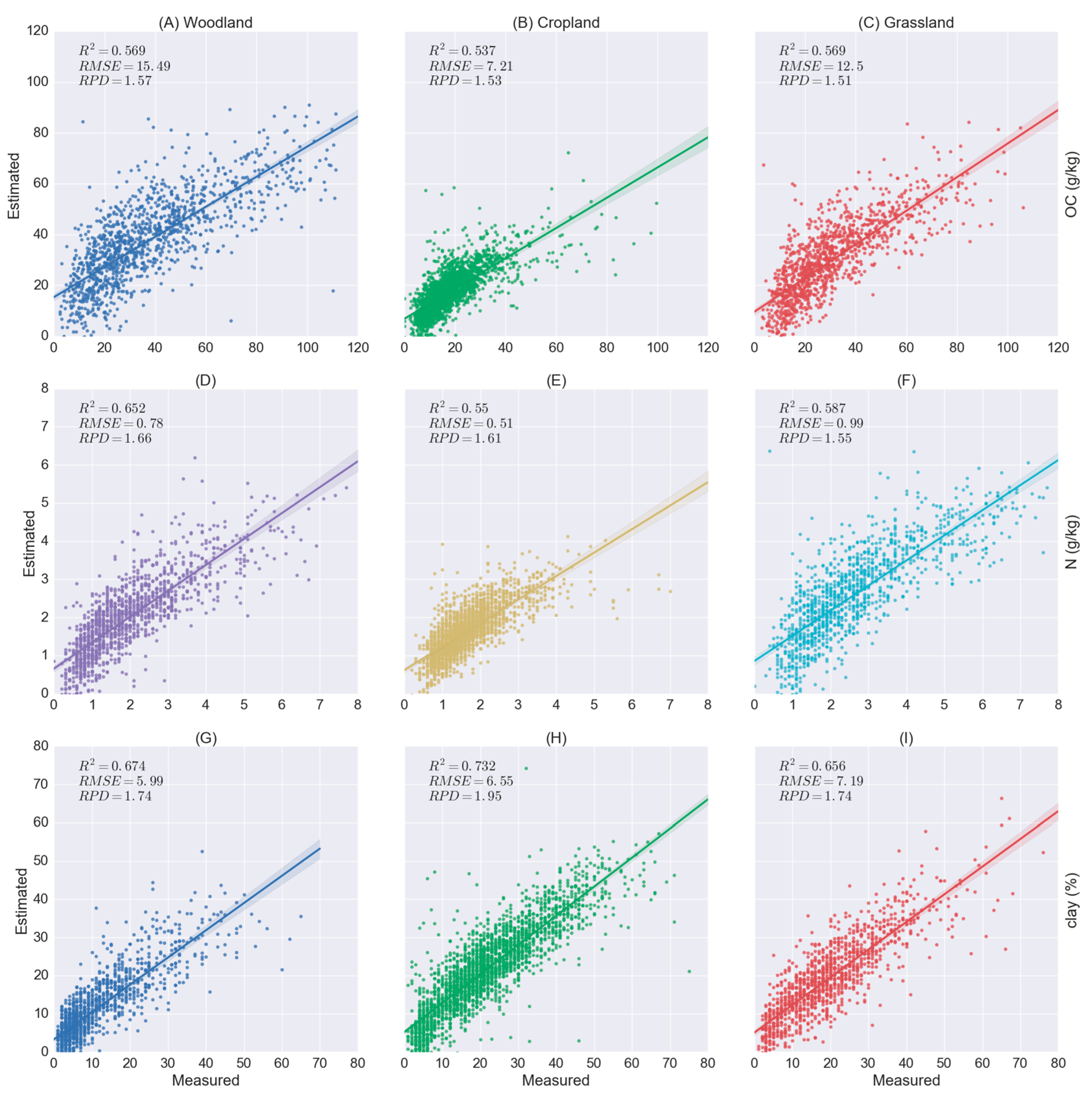
3.2. Results of PLS Regression for the Estimation of Soil Properties

To make a comparison with the following results obtained from PLS-GBDT, soil spectroscopic models for OC, N, and clay were developed using PLS regression with the same dataset (Figure 4). For each model, the PLS component number was optimised and kept the same as retained by PLS-GBDT (

Table 2. Optimised parameters for the spectroscopic model using the PLS-gradient-booted decision tree (GBDT) method.

Category	Property	PLS Components	Number of Trees	Maximum Depth
Woodland	OC (g/kg)	42	300	3
	N (g/kg)	78	1100	4
	Clay (%)	50	500	4
Cropland	OC (g/kg)	64	1950	4
	N (g/kg)	86	2000	4
	Clay (%)	82	2000	3
Grassland	OC (g/kg)	60	700	3
	N (g/kg)	72	900	3
	Clay (%)	60	1450	3

). The accuracies were assessed by R², RMSE, and RPD. Spectroscopic models developed for OC estimation achieved R² values ranging from 0.537 to 0.569 and RPD values from 1.51 to 1.57. For N, the highest accuracy (R² = 0.652, RMSE = 0.78 g/kg, RPD = 1.66) was obtained from woodland soils. Models developed for clay estimation achieved comparable good results, and R² values vary from 0.656 to 0.732. From RPD values, it can be seen that PLS regression can develop fair models for soil spectroscopic analysis that may be used for assessment and correlation.

Variable selection can be done with PLS. We use VIP scores to rank the relative variable importance. The top 60% variables were kept and further modelled with PLS regression. The results for all three soil categories were shown in Figure 5. After variable selection, the accuracy for clay estimation from woodland soils improved with retained variables (R² = 0.715, RMSE = 5.6 g/kg, RPD = 1.86) compared with using full spectrum (R² = 0.674, RMSE = 5.99 g/kg, RPD = 1.74). Variable selection can also increase the OC estimation accuracy for woodland soils. However, the estimation accuracies for clay from cropland soils and N from woodland soils decreased after variable selection. The R² values declined from 0.732 to 0.714 for clay (cropland soils) and 0.652 to 0.636 for N (woodland soils). Soil spectra is complex, especially for large-scale soil spectral data. Soil properties associated with spectrally active constituents cannot be expected to be globally stable [22]. Thus, directly dropping some bands via variable selection may result in a loss of information that is important for some soil samples.

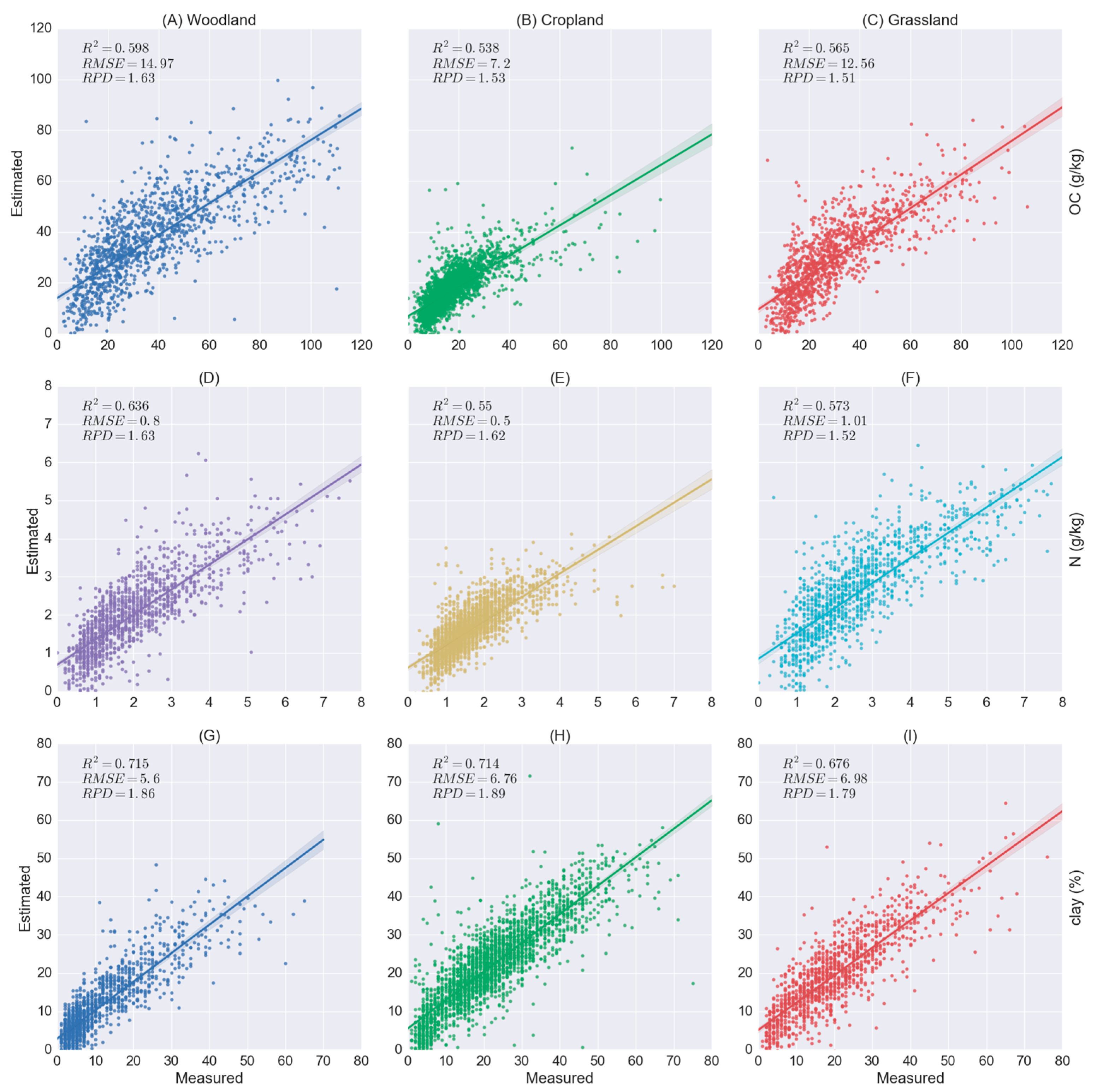
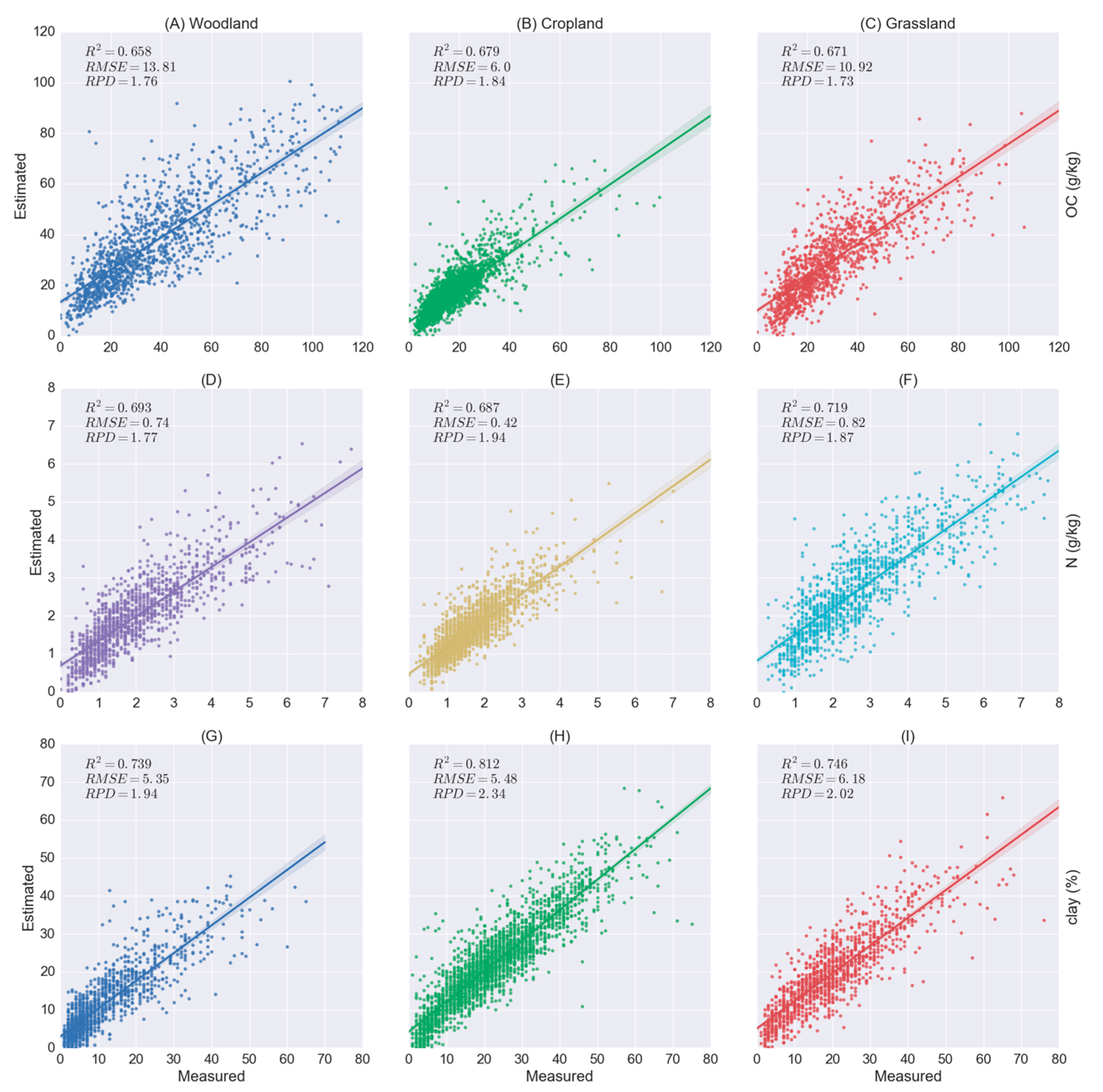
3.3. Results of PLS-GBDT for the Estimation of Soil Properties

In this study, we propose to transfer soil reflectance spectra data into PLS components so as to reduce the dimensionality and also decrease the computational complexity. Then, for each category (woodland, cropland, and grassland), soil properties of OC, N, and clay were modelled using the GBDT method while the input variables were PLS components instead of reflectance spectra. A grid search method was adopted to tune the optimised PLS components for the first step and also the number of boosted trees and the maximum tree depth for GBDT (Table 2).

For OC, the model built using cropland soil samples achieved the best result (R² = 0.679, RMSE = 6.0 g/kg, RPD = 1.84) compared with soil samples from woodland (R² = 0.658, RMSE = 13.81 g/kg, RPD = 1.76) and grassland (R² = 0.671, RMSE = 10.92 g/kg, RPD = 1.76), which is the same case for the other two soil properties. The spectroscopic model developed from cropland soils has a RPD value of 1.94 for N and 2.34 for clay, and both are higher than models developed for woodland soils and grassland soils. This might be due to the complexity of the soil sampling matrix and soil sampling density. From Figure 1, it can be seen that cropland soils have the largest proportion of samples because of their ease of access and thus distribute more homogenously compared with woodland soils and grassland soils. The accuracy of clay obtained from the developed PLS-GBDT model has the highest value compared with the other two properties, R² values ranging from 0.736 to 0.812 and RPD from 1.94 to 2.34.

Compared with Figure 4 and Figure 6, it can be clearly seen that the results achieved by PLS regression with or without variable selection are worse than by PLS-GBDT. For woodland soils, the R² value for OC reduced from 0.679 to 0.537 and the RPD value from 1.84 to 1.53, the R² value for N dropped from 0.687 to 0.55, the RPD value from 1.94 to 1.61, and the estimation of clay also has the same trend. Therefore, the model developed by non-linear regression method such as PLS-GBDT is suitable for quantitative retrieval of soil properties as reported by [3,44].

To further evaluate the performance of PLS-GBDT method, we also directly applied GBDT to soil reflectance spectra. We take samples from woodland soils as an example, and use the mean square error (MSE) as the evaluation metric. From Figure 7, it can be seen that GBDT model did not perform well, and it is not easy for it to be convergent with the increase of epochs in the training step, as the model tends to be complex when the data dimensionality is too high. PLS-GBDT models achieved much lower MSE values compared with GBDT models, both in the training and validation steps.

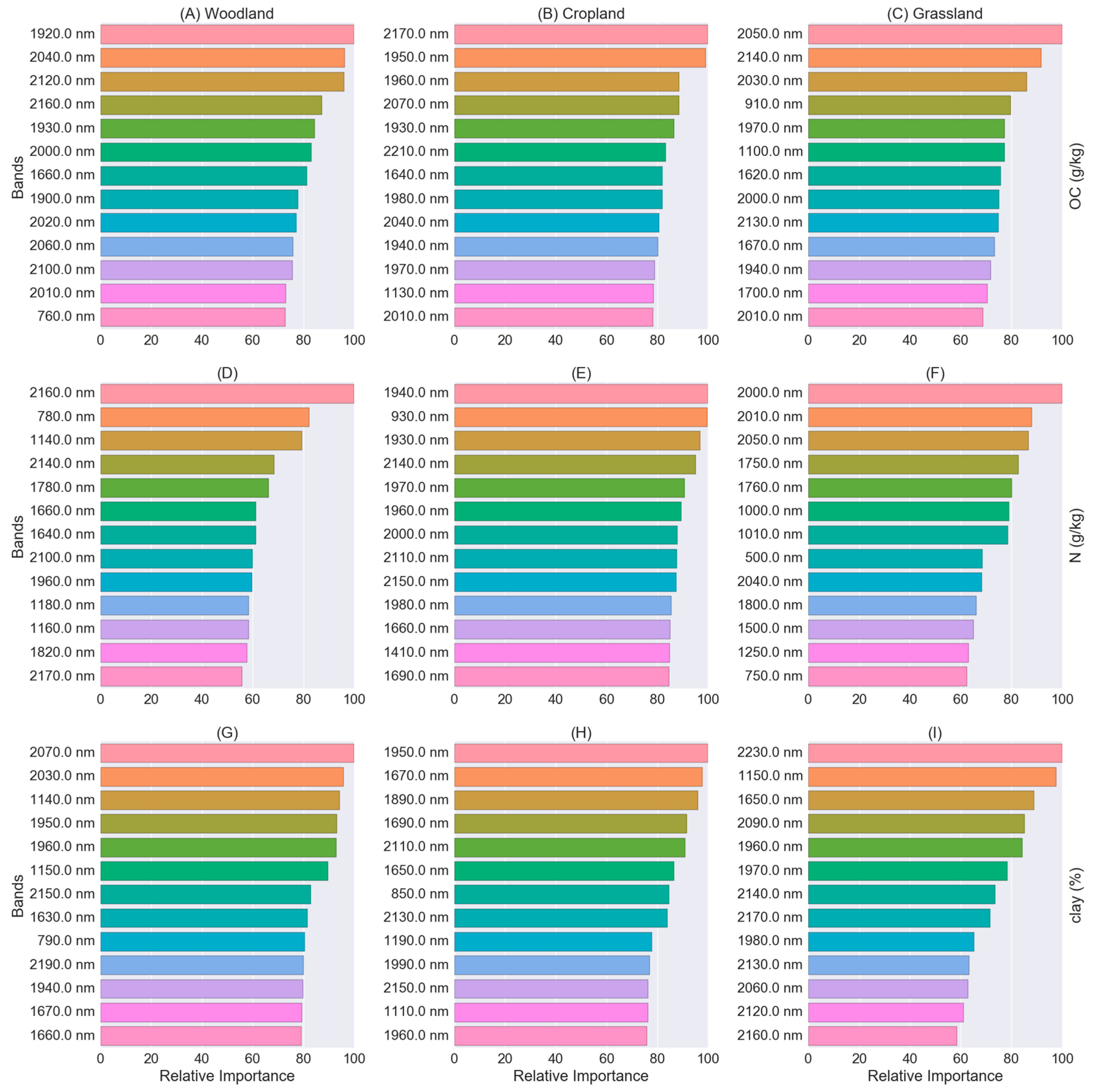
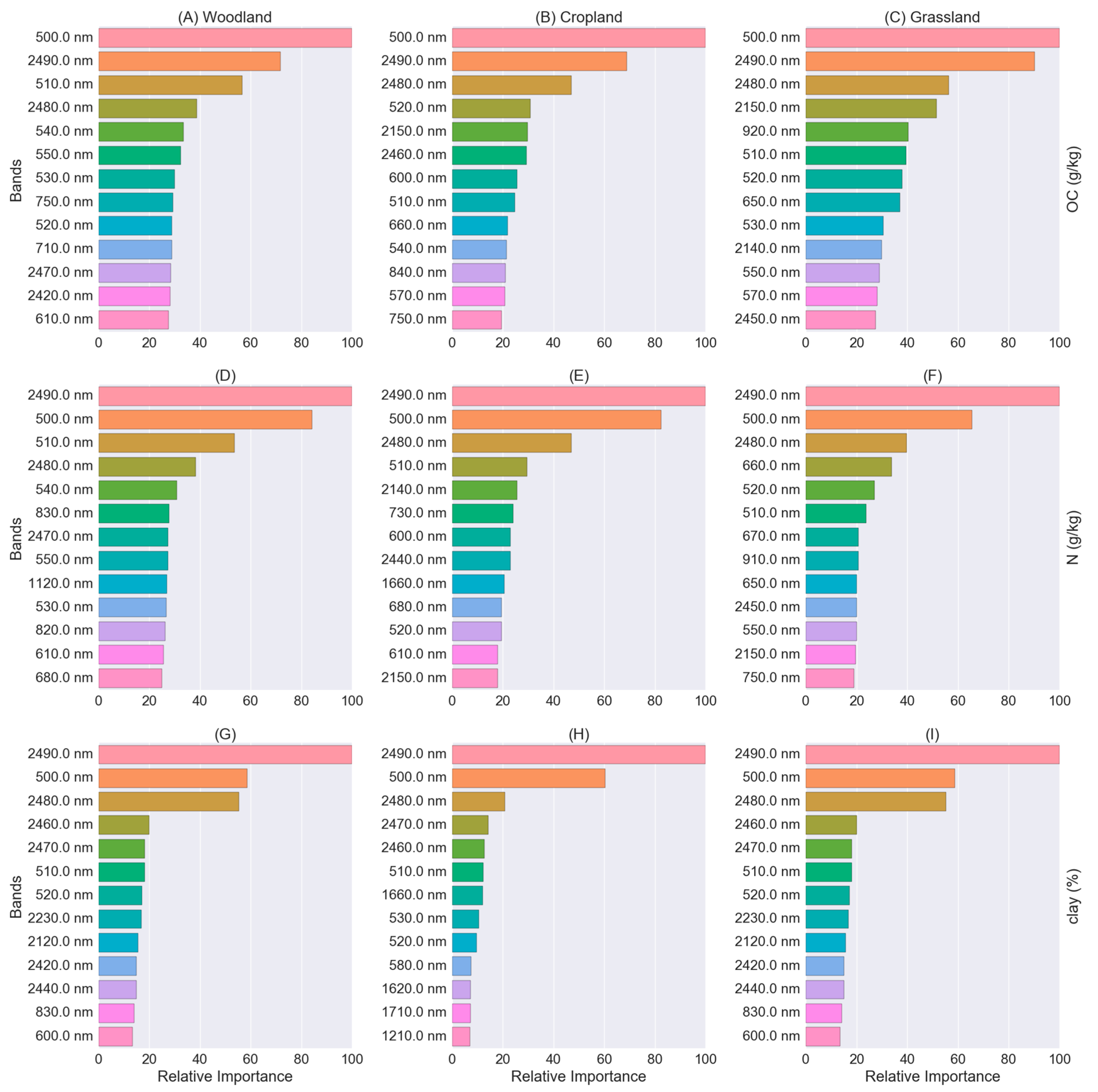
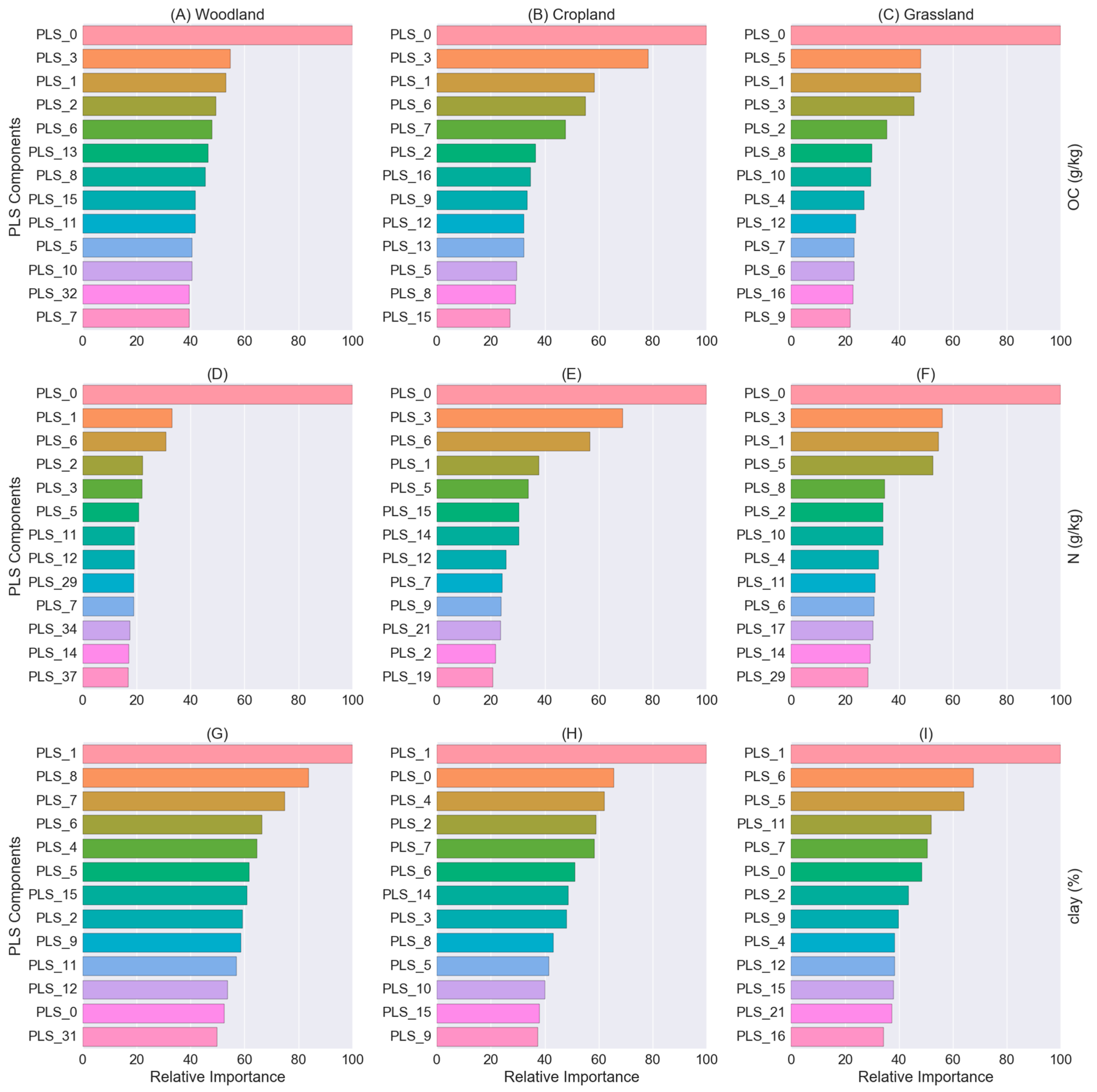
3.4. Relative Important Variables Derived from PLS Regression and the Gradient-Boosting Method

A benefit of PLS regression and GBDT is that they can provide the estimation of variable importance from the trained calibration model. As it is time consuming to tune hyperparameters for GBDT models with very high dimensional data, soil spectra were resampled to 200 bands. The top 13 relative important variables derived from PLS regression models can be seen from Figure 8. For OC, the most important bands for these three soil categories are at 1920, 2170, and 2050 nm. The top ranked bands for N are similar to OC (2160, 1940, and 2000 nm). For clay, the derived important variables are at 2070, 1950, and 2230 nm. In previous study [45], the bands near 800, 1000, 1400, and 1900–2450 nm were confirmed to be important for OC estimation, and the bands around 1100, 1600, 1700 to 1800, 2000, and 2200 to 2400 nm were also identified as key bands for OC and N estimation [46]. The results are basically in agreement with previous research.

For all of these three soil properties, the top ranked variables derived from GBDT model were basically at the beginning and the end of the spectrum (Figure 9). It can be seen that the GBDT method failed to select meaningful bands for quantitative estimation of OC, N, and clay when directly using the full spectrum as an input variable, which also explained why the accuracy of the GBDT model is worse than the results obtained from PLS and PLS-GBDT models. Conversely, relative important variables derived from PLS regression are more reasonable.

Although the GBDT method failed to derive the relative important variables when using full spectrum, it does not mean that this method is not suitable for soil spectroscopic analysis. The obtained relative important variables were demonstrated (Figure 10) when the model was combined with retained PLS components. For PLS-GBDT, the first PLS component is supposed to be the most important variable for the estimation of corresponding soil properties, as PLS retains target-related information. The results demonstrate that the most important variables are the first PLS component for OC and N, while the second PLS component is ranked first for clay. In general, the top-ranked PLS components are also important to the gradient-boosting model, as revealed by Figure 10. This also means that PLS performs well on the extraction of target-related information.

4. Discussion

4.1. Dimension Reduction for High-Dimensional Soil Spectra

High-dimensional data like soil spectra often contain redundant information and will increase computation complexity, which is known as the curse of dimensionality or Hughes phenomenon [47,48,49]. Variable selection can reduce the complexity and improve the robustness of the model. By selecting the most informative spectral bands instead of using the full spectrum, the calibration model is supposed to be more accurate [50]. Variable selection can be based on physical background by identifying key wavelengths for the target property. It is also possible to evaluate it using the statistics of the resulting calibration model, like the VIP score derived from the PLS regression model in this study.

High-dimensional spectral data can be projected to a lower dimensional space without actually losing significant information using methods like principal component analysis (PCA). PCA reduces the dimensionality of the data to fewer components that describe a large proportion of the variance. The first principal component accounts for the largest variance, while subsequent components account for decreasingly smaller proportions [51]. Local linear embedding (LLE) is a nonlinear dimensionality reduction method, and it can identify the underlying structure of a manifold [52]. PCA and LLE have been exploited in a comparative way for soil spectral distance and similarity in projected space [53]. Autoencoder (AE) is an unsupervised learning algorithm and its performance on reducing the dimensionality of soil spectra has not been well studied. Several approaches were developed based on it, such as stacked autoencoder and sparse autoencoder [54,55]. AE trains a neural network by constraining the output values to be equal to the input values. The reconstruction error between the input and the output is used to adjust the weights of each layer. Ideally, features learned by AE can well represent the input data [56]. The difference between PLS and the above mentioned DR methods is that PLS is able to retain target-related information and can be viewed as a supervised DR method. It has the potential to explore the intrinsic structure of spectra, and it not only reduces data redundancy, it also improves estimation accuracy. Besides, it is worth making a comparison between PLS and other mentioned DR methods (PCA, LLE, AE, etc.) for soil spectral analysis in the following studies.

4.2. GBDT for Quantitative Soil Spectroscopic Modelling

Modelling soil properties using large and diverse soil spectral libraries is still a challenging task. PLS regression, as a common approach in soil spectroscopy, has limitations in handling large-scale soil spectral data. With variable selection using VIP scores, the performance with regard to improving the estimation accuracies is still not satisfying in this study. GBDT has been used to win machine learning competitions on Kaggle and has gained a lot of attention. In this study, we proposed to take advantage of GBDT for the estimation of soil properties by using PLS components as the input variables instead of raw reflectance spectra. The result demonstrated that the combined PLS-GBDT approach performs better than PLS or GBDT alone. It also confirmed the experiments in [57], in which the boosted decision trees method performed exceptionally well when dimensionality was low. The model is prone to being complex when the dimension is too high, and it tends to need more trees and a high degree of tree depth, which could be a serious problem in high dimensions [58]. Therefore, it is suggested to reduce the number of input features via dimension reduction or feature selection when facing high-dimensional data. There are several studies related to soil spectroscopic modelling using large-scale soil spectral libraries. Local or MBL approaches are reputed to have better performance on large-scale soil data. PLS, SVM, LWR, and SBL were comparatively studied on a regional soil spectral library in Brazil and a global soil spectral library [22]. SBL algorithm achieved the best performance for OC estimation in the regional (R² = 0.59) and the global data (R² = 0.68). MBL approaches are very flexible and can be easily integrated with PLS-GBDT. Besides, additional soil information like texture (sand, clay, and silt) can contribute to soil spectroscopic model. By only using spectral bands as the input variables in [59], SVM obtained a similar result for OC estimation of cropland soils as achieved by PLS-GBDT. However, the R² value improved from 0.67 to 0.71 with variable selection and clay content as auxiliary variable. A higher accuracy of the OC estimation model was also obtained by [60] when considering sand content. Therefore, additional soil information is very important to calibration models for large-scale soil spectral data.

5. Conclusions

Soil spectra measured in the laboratory typical have several hundred or even thousand bands, which would be a problem for the gradient-boosting model when directly using such high-dimensional data as inputs. This study presents a PLS-GBDT method to retrieve soil properties from reflectance spectra. The LUCAS soil spectral library was used to evaluate its performance. For three soil categories (woodland, grassland, and cropland), R² achieved values of 0.658–0.679 for OC, 0.687–0.719 for N, and 0.739–0.812 for clay. Both PLS and GBDT can estimate the relative contributions of input variables. However, GBDT failed in this task when directly using high-dimensional soil spectra as input data. The GBDT method is a well-known machine learning algorithm that uses the decision tree as the weak learner, and it has successfully been applied in numerous areas. By using PLS components as input variables, which are retained with target variable-related information, GBDT is able to perform well on soil quantitative analysis. Although the PLS-GBDT method is directly used to develop a global model to fit the whole soil spectral library in this study, it is possible to combine it with MBL if it functions as a basic or local model.

References

1. Nocita, M.; Stevens, A.; van Wesemael, B.; Aitkenhead, M.; Bachmann, M.; Barthès, B.; Ben-Dor, E.; Brown, D.J.; Clairotte, M.; Csorba, A.; et al. Soil spectroscopy: An alternative to wet chemistry for soil monitoring. Adv. Agron. 2015, 132, 139–159. [Google Scholar]
2. Soriano-Disla, J.M.; Janik, L.J.; Viscarra Rossel, R.A.; MacDonald, L.M.; McLaughlin, M.J. The performance of visible, near-, and mid-infrared reflectance spectroscopy for prediction of soil physical, chemical, and biological properties. Appl. Spectrosc. Rev. 2014, 49, 139–186. [Google Scholar] [CrossRef]
3. Viscarra Rossel, R.A.; Behrens, T.; Ben-Dor, E.; Brown, D.J.; Demattê, J.A.M.; Shepherd, K.D.; Shi, Z.; Stenberg, B.; Stevens, A.; Adamchuk, V.; et al. A global spectral library to characterize the world’s soil. Earth-Sci. Rev. 2016, 155, 198–230. [Google Scholar] [CrossRef] [Green Version]
4. Wang, Y.; Huang, T.; Liu, J.; Lin, Z.; Li, S.; Wang, R.; Ge, Y. Soil pH value, organic matter and macronutrients contents prediction using optical diffuse reflectance spectroscopy. Comput. Electron. Agric. 2015, 111, 69–77. [Google Scholar] [CrossRef]
5. Shi, Z.; Wang, Q.L.; Peng, J.; Ji, W.; Liu, H.J.; Li, X.; Viscarra Rossel, R.A. Development of a national VNIR soil-spectral library for soil classification and prediction of organic matter concentrations. Sci. China Earth Sci. 2014, 57, 1671–1680. [Google Scholar] [CrossRef]
6. Ben-Dor, E.; Chabrillat, S.; Demattê, J.A.M.; Taylor, G.R.; Hill, J.; Whiting, M.L.; Sommer, S. Using imaging spectroscopy to study soil properties. Remote Sens. Environ. 2009, 113, S38–S55. [Google Scholar] [CrossRef]
7. Nocita, M.; Stevens, A.; van Wesemael, B.; Brown, D.J.; Shepherd, K.D.; Towett, E.; Vargas, R.; Montanarella, L. Soil spectroscopy: An opportunity to be seized. Glob. Chang. Biol. 2015, 21, 10–11. [Google Scholar] [CrossRef] [PubMed]
8. Ben-Dor, E.; Banin, A. Near-Infrared analysis as a rapid method to simultaneously evaluate several Soil properties. Soil Sci. Soc. Am. J. 1995, 59, 364–372. [Google Scholar] [CrossRef]
9. Wang, J.; Cui, L.; Gao, W.; Shi, T.; Chen, Y.; Gao, Y. Prediction of low heavy metal concentrations in agricultural soils using visible and near-infrared reflectance spectroscopy. Geoderma 2014, 216, 1–9. [Google Scholar] [CrossRef]
10. Ben-Dor, E.; Patkin, K.; Richter, R.; Mueller, A.; Kaufmann, H. Mapping of several soil properties using DAIS-7915. In A Decade of Trans-European Remote Sensing Cooperation; Buchroithner, M., Ed.; CRC Press: Dresden, Germany, 2001; pp. 385–390. [Google Scholar]
11. Kopačková, V.; Ben-Dor, E.; Carmon, N.; Notesco, G. Modelling diverse soil attributes with visible to longwave infrared spectroscopy using PLSR employed by an automatic modelling engine. Remote Sens. 2017, 9, 134. [Google Scholar] [CrossRef]
12. Leone, A.; Viscarra-Rossel, R.A.; Amenta, P.; Buondonno, A. Prediction of soil properties with PLSR and vis-NIR spectroscopy: Application to mediterranean soils from Southern Italy. Curr. Anal. Chem. 2012, 8, 283–299. [Google Scholar] [CrossRef]
13. Gholizadeh, A.; Carmon, N.; Klement, A.; Ben-Dor, E.; Borůvka, L. Agricultural Soil Spectral Response and Properties Assessment: Effects of Measurement Protocol and Data Mining Technique. Remote Sens. 2017, 9, 1078. [Google Scholar] [CrossRef]
14. Steinberg, A.; Chabrillat, S.; Stevens, A.; Segl, K.; Foerster, S. Prediction of common surface soil properties based on Vis-NIR airborne and simulated EnMAP imaging spectroscopy data: Prediction accuracy and influence of spatial resolution. Remote Sens. 2016, 8, 613. [Google Scholar] [CrossRef]
15. Tran, T.N.; Afanador, N.L.; Buydens, L.M.C.; Blanchet, L. Interpretation of variable importance in partial least squares with significance multivariate correlation (sMC). Chemom. Intell. Lab. Syst. 2014, 138, 153–160. [Google Scholar] [CrossRef]
16. Li, X.; Zhang, Y.; Bao, Y.; Luo, J.; Jin, X.; Xu, X.; Song, X.; Yang, G. Exploring the best hyperspectral features for LAI estimation using partial least squares regression. Remote Sens. 2014, 6, 6221–6241. [Google Scholar] [CrossRef]
17. Mehmood, T.; Liland, K.H.; Snipen, L.; Sæbø, S. A review of variable selection methods in partial least squares regression. Chemom. Intell. Lab. Syst. 2012, 118, 62–69. [Google Scholar] [CrossRef]
18. Norgaard, L.; Wagner, J.; Nielsen, J.P.; Munc, L.; Engelsen, S.B. Interval partial least-squares regression (iPLS): A comparative chemometric study with an example from near-infrared spectroscopy. Appl. Spectrosc. 2000, 54, 413–419. [Google Scholar] [CrossRef]
19. Vohland, M.; Besold, J.; Hill, J.; Fründ, H.-C. Comparing different multivariate calibration methods for the determination of soil organic carbon pools with visible to near infrared spectroscopy. Geoderma 2011, 166, 198–205. [Google Scholar] [CrossRef]
20. Christy, C.D.; Dyer, S.A. Estimation of soil properties using a combination of spectral and scalar sensor data. In 2006 IEEE Instrumentation and Measurement Technology Conference Proceedings; IEEE: New York, NY, USA, 2006; pp. 729–734. [Google Scholar]
21. Gogé, F.; Joffre, R.; Jolivet, C.; Ross, I.; Ranjard, L. Optimization criteria in sample selection step of local regression for quantitative analysis of large soil NIRS database. Chemom. Intell. Lab. Syst. 2012, 110, 168–176. [Google Scholar] [CrossRef]
22. Ramirez-Lopez, L.; Behrens, T.; Schmidt, K.; Stevens, A.; Demattê, J.A.M.; Scholten, T. The spectrum-based learner: A new local approach for modeling soil vis-NIR spectra of complex datasets. Geoderma 2013, 195, 268–279. [Google Scholar] [CrossRef]
23. Gholizadeh, A.; Borůvka, L.; Saberioon, M.; Vašát, R. A memory-based learning approach as compared to other data mining algorithms for the prediction of soil texture using diffuse reflectance spectra. Remote Sens. 2016, 8, 341. [Google Scholar] [CrossRef]
24. Bu, H.L.; Li, G.Z.; Zeng, X.Q.; Yang, J.Y.; Yang, M.Q. Feature selection and partial least squares based dimension reduction for tumor classification. In Proceedings of the 7th IEEE International Conference on Bioinformatics and Bioengineering, Boston, MA, USA, 14–17 October 2007; pp. 967–973. [Google Scholar]
25. Boulesteix, A.-L. PLS dimension reduction for classification with microarray data. Stat. Appl. Genet. Mol. Biol. 2004, 3, 1–30. [Google Scholar] [CrossRef] [PubMed] [Green Version]
26. Liu, Y.; Rayens, W. PLS and dimension reduction for classification. Comput. Stat. 2007, 22, 189–208. [Google Scholar] [CrossRef]
27. Tang, L.; Peng, S.; Bi, Y.; Shan, P.; Hu, X. A new method combining LDA and PLS for dimension reduction. PLoS ONE 2014, 9, e96944. [Google Scholar] [CrossRef] [PubMed]
28. Rosipal, R.; Krämer, N. Overview and recent advances in partial least squares. In Subspace, Latent Structure and Feature Selection; Springer: Berlin/Heidelberg, Germany, 2006; pp. 34–51. [Google Scholar]
29. Höskuldsson, A. PLS regression methods. J. Chemom. 1988, 2, 211–228. [Google Scholar] [CrossRef]
30. Chen, T.; Guestrin, C. XGBoost: Reliable large-scale tree boosting system. In Proceedings of the 22nd SIGKDD Conference on Knowledge Discovery and Data Mining, San Francisco, CA, USA, 13–17 August 2016. [Google Scholar]
31. Agrawal, R.J.; Shanahan, J.G. Location disambiguation in local searches using gradient boosted decision trees. In Proceedings of the 18th SIGSPATIAL International Conference on Advances in Geographic Information Systems, San Jose, CA, USA, 3–5 November 2010; pp. 129–136. [Google Scholar]
32. Mitchell, R.; Frank, E. Accelerating the XGBoost algorithm using GPU computing. PeerJ Prepr. 2017, 5, e2911v1. [Google Scholar] [CrossRef]
33. Tóth, G.; Jones, A.; Montanarella, L. LUCAS Topsoil Survey: Methodology, Data, and Results; Publications Office: Luxembourg, 2013. [Google Scholar]
34. Tóth, G.; Jones, A.; Montanarella, L. The LUCAS topsoil database and derived information on the regional variability of cropland topsoil properties in the European Union. Environ. Monit. Assess. 2013, 185, 7409–7425. [Google Scholar] [CrossRef] [PubMed]
35. Friedman, J.H. Greedy function approximation: A gradient boosting machine. Ann. Stat. 2001, 29, 1189–1232. [Google Scholar] [CrossRef]
36. Friedman, J.H. Stochastic Gradient Boosting. Comput. Stat. Data Anal. 2002, 38, 367–378. [Google Scholar] [CrossRef]
37. Chopra, T.; Vajpai, J. Fault diagnosis in benchmark process control system using stochastic gradient boosted decision trees. Int. J. Soft Comput. Eng. 2011, 1, 98–101. [Google Scholar]
38. Ke, G.; Meng, Q.; Finley, T.; Wang, T.; Chen, W.; Ma, W.; Ye, Q.; Liu, T. LightGBM: A highly efficient gradient boosting decision tree. In Advances in Neural Information Processing Systems; Morgan Kaufmann Publishers: San Mateo, CA, USA, 2017; pp. 3148–3156. [Google Scholar]
39. Pedregosa, F.; Weiss, R.; Brucher, M. Scikit-learn: Machine learning in Python. J. Mach. Learn. Res. 2011, 12, 2825–2830. [Google Scholar]
40. LightGBM. Available online: https://github.com/Microsoft/LightGBM/ (accessed on 10 December 2017).
41. Zhu, J.; Shan, Y.; Mao, J.; Yu, D.; Rahmanian, H.; Zhang, Y. Deep embedding forest: Forest-based serving with deep embedding features. In Proceedings of the ACM SIGKDD International Conference on Knowledge Discovery and Data Mining, Halifax, NS, USA, 13–17 August 2017. [Google Scholar]
42. Viscarra Rossel, R.A.; McGlynn, R.N.; McBratney, A.B. Determining the composition of mineral-organic mixes using UV-vis-NIR diffuse reflectance spectroscopy. Geoderma 2006, 137, 70–82. [Google Scholar] [CrossRef]
43. Ben-Dor, E.; Taylor, R.G.; Hill, J.; Demattê, J.A.M.; Whiting, M.L.; Chabrillat, S.; Sommer, S. Imaging spectrometry for soil applications. Adv. Agron. 2008, 97, 321–392. [Google Scholar]
44. Viscarra Rossel, R.A.; Walvoort, D.J.J.; McBratney, A.B.; Janik, L.J.; Skjemstad, J.O. Visible, near infrared, mid infrared or combined diffuse reflectance spectroscopy for simultaneous assessment of various soil properties. Geoderma 2006, 131, 59–75. [Google Scholar] [CrossRef]
45. Peng, X.; Shi, T.; Song, A.; Chen, Y.; Gao, W. Estimating soil organic carbon using VIS/NIR spectroscopy with SVMR and SPA methods. Remote Sens. 2014, 6, 2699–2717. [Google Scholar] [CrossRef]
46. Stenberg, B.; Viscarra Rossel, R.A.; Mouazen, A.M.; Wetterlind, J. Visible and near infrared spectroscopy in soil science. Adv. Agron. 2010, 107, 163–215. [Google Scholar]
47. Mukherjee, K.; Ghosh, J.K.; Mittal, R.C. Dimensionality reduction of hyperspectral data using spectral fractal feature. Geocarto Int. 2012, 27, 515–531. [Google Scholar] [CrossRef]
48. Huang, H.; Luo, F.; Liu, J.; Yang, Y. Dimensionality reduction of hyperspectral images based on sparse discriminant manifold embedding. ISPRS J. Photogramm. Remote Sens. 2015, 106, 42–54. [Google Scholar] [CrossRef]
49. Liu, L.; Ji, M.; Dong, Y.; Zhang, R.; Buchroithner, M. Quantitative retrieval of organic soil properties from visible near-infrared Shortwave infrared (Vis-NIR-SWIR) spectroscopy feature extraction. Remote Sens. 2016, 8, 1035. [Google Scholar] [CrossRef]
50. Vohland, M.; Ludwig, M.; Thiele-bruhn, S.; Ludwig, B. Determination of soil properties with visible to near- and mid-infrared spectroscopy: Effects of spectral variable selection. Geoderma 2014, 223–225, 88–96. [Google Scholar] [CrossRef]
51. Viscarra Rossel, R.A.; Chappell, A.; De Caritat, P.; Mckenzie, N.J. On the soil information content of visible-near infrared reflectance spectra. Eur. J. Soil Sci. 2011, 62, 442–453. [Google Scholar] [CrossRef]
52. Roweis, S. Nonlinear dimensionality reduction by locally linear embedding. Science 2000, 290, 2323–2326. [Google Scholar] [CrossRef] [PubMed]
53. Ramirez-lopez, L.; Behrens, T.; Schmidt, K.; Viscarra Rossel, R.A.; Demattê, J.A.M.; Scholten, T. Distance and similarity-search metrics for use with soil vis-NIR spectra. Geoderma 2013, 199, 43–53. [Google Scholar] [CrossRef]
54. Zhang, L.; Zhang, L.; Kumar, V. Deep learning for Remote Sensing Data:A technical tutorial on the state of the art. IEEE Geosci. Remote Sens. Mag. 2016, 18, 22–40. [Google Scholar] [CrossRef]
55. Vincent, P.; Larochelle, H.; Lajoie, I.; Bengio, Y. Pierre-AntoineManzagol Stacked denoising autoencoders: Learning useful representations in a deep network with a local denoising criterion. J. Mach. Learn. Res. 2010, 11, 3371–3408. [Google Scholar]
56. Xing, C.; Ma, L.; Yang, X. Stacked denoise autoencoder based feature extraction and classification for hyperspectral images. J. Sens. 2015, 2016, 3632943. [Google Scholar] [CrossRef]
57. Caruana, R.; Niculescu-Mizil, A. An empirical comparison of supervised learning algorithms. In Proceedings of the 23rd International Conference on Machine Learning, Pittsburgh, PA, USA, 25–29 June 2006; pp. 161–168. [Google Scholar]
58. Caruana, R.; Karampatziakis, N.; Yessenalina, A. An empirical evaluation of supervised learning in high dimensions. In Proceedings of the 25th International Conference on Machine Learning, Helsinki, Finland, 5–9 July 2008; pp. 96–103. [Google Scholar]
59. Stevens, A.; Nocita, M.; Tóth, G.; Montanarella, L.; van Wesemael, B. Prediction of soil organic carbon at the European scale by visible and near infraRed reflectance spectroscopy. PLoS ONE 2013, 8, e66409. [Google Scholar] [CrossRef] [PubMed]
60. Nocita, M.; Stevens, A.; Toth, G.; Panagos, P.; van Wesemael, B.; Montanarella, L. Prediction of soil organic carbon content by diffuse reflectance spectroscopy using a local partial least square regression approach. Soil Biol. Biochem. 2014, 68, 337–347. [Google Scholar] [CrossRef]
Figure 1. Location of selected soil samples from the Land Use/Land Cover Area Frame Survey (LUCAS) soil spectral library. The colour indicates the corresponding land cover type.
Remotesensing 09 01299 g001
Figure 2. Illustration of level-wise and leaf-wise tree growth approaches for gradient-boosted decision trees.
Remotesensing 09 01299 g002
Figure 3. (AC) are mean soil reflectance spectra (black lines) and standard deviations (blue lines, lower and upper boundaries) for soil samples from woodland, cropland, and grassland; (DF) are mean soil continuum-removal spectra (black lines) and standard deviations (blue lines, lower and upper boundaries) for soil samples from woodland, cropland, and grassland. Values are given in reflectance (AC) and normalized continuum-removal values (DF).
Remotesensing 09 01299 g003
Figure 4. Results of soil property estimation accuracies using the partial least squares (PLS) regression method. (AC) are organic carbon accuracies for samples from woodland, cropland, and grassland soils, and (DF) are N accuracies, and (GI) are clay accuracies.
Remotesensing 09 01299 g004
Figure 5. Results of soil property estimation accuracies using PLS regression with variable selection using VIP scores. (AC) are organic carbon accuracies for samples from woodland, cropland, and grassland soils, and (DF) are N accuracies, and (GI) are clay accuracies.
Remotesensing 09 01299 g005
Figure 6. Results of soil property estimation accuracies using the PLS gradient-boosting regression method. (AC) are organic carbon accuracies for samples from woodland, cropland, and grassland soils, and (DF) are N accuracies, and (GI) are clay accuracies.
Remotesensing 09 01299 g006
Figure 7. Training and validation curves of soil spectroscopic models developed by PLS-GDBT (AC) and GBDT (DF) in 500 epochs for woodland soil samples.
Remotesensing 09 01299 g007
Figure 8. The top 13 relative important variables derived from PLS regression models. (AC) are relative important variables derived from OC models for woodland, cropland, and grassland soils, and (DF) are relative important variables derived from N models, and (GI) are relative important variables derived from clay models.
Remotesensing 09 01299 g008
Figure 9. The top 13 relative important variables derived from GBDT models. (AC) are relative important variables derived from OC models for woodland, cropland, and grassland soils, and (DF) are relative important variables derived from N models, and (GI) are relative important variables derived from clay models.
Remotesensing 09 01299 g009
Figure 10. The top 13 relative important variables (PLS components) derived from PLS-GBDT. (AC) are relative important variables derived from OC models for woodland, cropland, and grassland soils, and (DF) are relative important variables derived from N models, and (GI) are relative important variables derived from clay models.
Remotesensing 09 01299 g010