Using Worldview Satellite Imagery to Map Yield in Avocado (Persea americana): A Case Study in Bundaberg, Australia


Agricultural Remote Sensing Team, Precision Agriculture Research Group, University of New England, Armidale, NSW 2350, Australia
*
Author to whom correspondence should be addressed.
Remote Sens. 2017, 9(12), 1223; https://doi.org/10.3390/rs9121223
Submission received: 6 October 2017
/
Revised: 21 November 2017
/
Accepted: 21 November 2017
/
Published: 27 November 2017
(This article belongs to the Section Remote Sensing in Agriculture and Vegetation)
Abstract
:Accurate pre-harvest estimation of avocado (Persea americana cv. Haas) yield offers a range of benefits to industry and growers. Currently there is no commercial yield monitor available for avocado tree crops and the manual count method used for yield forecasting can be highly inaccurate. Remote sensing using satellite imagery offers a potential means to achieve accurate pre-harvest yield forecasting. This study evaluated the accuracies of high resolution WorldView (WV) 2 and 3 satellite imagery and targeted field sampling for the pre-harvest prediction of total fruit weight (kg·tree−1) and average fruit size (g) and for mapping the spatial distribution of these yield parameters across the orchard block. WV 2 satellite imagery was acquired over two avocado orchards during 2014, and WV3 imagery was acquired in 2016 and 2017 over these same two orchards plus an additional three orchards. Sample trees representing high, medium and low vigour zones were selected from normalised difference vegetation index (NDVI) derived from the WV images and sampled for total fruit weight (kg·tree−1) and average fruit size (g) per tree. For each sample tree, spectral reflectance data was extracted from the eight band multispectral WV imagery and 18 vegetation indices (VIs) derived. Principal component analysis (PCA) and non-linear regression analysis was applied to each of the derived VIs to determine the index with the strongest relationship to the measured total fruit weight and average fruit size. For all trees measured over the three year period (2014, 2016, and 2017) a consistent positive relationship was identified between the VI using near infrared band one and the red edge band (RENDVI1) to both total fruit weight (kg·tree−1) (R2 = 0.45, 0.28, and 0.29 respectively) and average fruit size (g) (R2 = 0.56, 0.37, and 0.29 respectively) across all orchard blocks. Separate analysis of each orchard block produced higher R2 values as well as identifying different optimal VIs for each orchard block and year. This suggests orchard location and growing season are influencing the relationship of spectral reflectance to total fruit weight and average fruit size. Classified maps of avocado yield (kg·tree−1) and average fruit size per tree (g) were produced using the relationships developed for each orchard block. Using the relationships derived between the measured yield parameters and the optimal VIs, total fruit yield (kg) was calculated for each of the five sampled blocks for the 2016 and 2017 seasons and compared to actual yield at time of harvest and pre-season grower estimates. Prediction accuracies achieved for each block far exceeded those provided by the grower estimates.

1. Introduction
Accurate pre-harvest yield parameter estimation in high value fruit tree crops, such as avocado (Persea americana cv. Haas), offers improved decision making from the grower to the industry level. For individual orchards, a strong understanding of yield variability allows growers to form improved decisions regarding the variable rate application of inputs (water, fertilizer, pesticides) and the logistical planning of field operations (e.g., harvest scheduling, number of pickers and bins required, etc.) [1,2,3]. At the start of the picking season when the price of high quality fruit is at its premium, an understanding of fruit size distribution across an orchard prior to harvest can greatly reduce labour and fuel costs through selective harvesting [4]. Additionally, accurate yield estimation during a growing season supports post-harvest decisions such as the storage, handling, packing, and forward selling of produce [4,5].
Currently, yield estimation in avocado orchards is undertaken by the visual counting of fruit growing on a small number of selected trees [4]. However, this method possesses several disadvantages: (1) poor accuracy as the avocado fruit is often occluded by leaves that are the same colour and shape; (2) time consuming and labour intensive, with many man hours required to undertake the counts on selected trees; (3) limited sample size, with the trees selected not accurately representing the high spatial and temporal variability of an entire orchard block.
Crop simulation models have been developed for a number of tree crops to estimate fruit number based on (i) yield capacity, (ii) average fruit set density, and (iii) average weight of the fruit at harvest. The ‘Bavendorf Crop Estimation Model’ initially developed by Winter [6] for apple and pear orchards was later evaluated for avocado by Köhne [3]. However, these methods are only conducted on a limited number of sample trees and therefore suffer the same inaccuracies as those identified by the visual count technique. Aggelopoulou et al. [7] and Alburquerque et al. [8] identified empirical relationships between fruit yield to number of new leaves and to number of flower buds after thinning in the spring. However, highly erroneous results occurred when the thinning process was not completed by spring. Whiley et al. [9] developed a ‘pheno-physiological model’ for ‘cv. Haas’ avocado grown in south-eastern Queensland Australia to establish a stronger understanding between physiological status of the tree in terms of its vegetative (roots and shoots) and reproductive (flowers and fruit) components to growth parameters including fruit set, fruit retention and yield. A relationship between the level of starch concentration in the tissues of the tree trunks immediately prior to flowering and subsequent fruit yield was identified. However, the occurrence of additional biotic or abiotic conditions between final crop set and harvest largely influenced the prediction accuracy.
Digital imaging or machine-vision techniques using stereo and colour photographs have also been investigated for yield estimation and/or real-time yield mapping of a number of horticultural crops including wild blueberries [10] and ‘Gala’ apple [11]. However, occlusion of fruit by branches and leaves, variations in illumination conditions, and thresholding errors were identified to be sources of error [12,13,14,15]. For avocado, fruit occlusion is likely to cause similar issues due to the leaves being the same shape and colour as the fruit, the fruit themselves growing inside the canopy, and the size of trees.
Satellite and aerial remote sensing platforms present as an accurate and time efficient alternative to the manual fruit count method [4] and for the non- invasive measure of avocado yield. Whilst these technologies have been found to be highly effective for measuring yield in row crops [16,17,18,19,20], generally attributed to harvest index (HI) (i.e., fraction of biomass allocated to yield components divided by the total above ground biomass) [21,22,23], similar studies in perennial fruit tree crops, such as citrus [24,25], apple [7,26], pear [27], peach [28], olives [28], mango [29], and grapevines [30,31] have produced varying levels of success. For avocado, there has only been limited remote sensing research investigating fruit size and yield mapping as well as tree number auditing [4]. It is hypothesised that remote sensing may provide an accurate measure of avocado yield via the relationship between tree canopy size/health measured after final fruit set.
The recent advent of very high resolution (VHR) satellites, such as WorldView-2 (WV2) (1.85 m multispectral resolution), WorldView-3 (WV3) (1.2 m multispectral resolution) and GeoEYE-1 (1.84 m resolution), allows the spectral reflectance characteristics of individual tree canopies to be measured. Additionally, the increased spectral resolution of these sensors i.e., up to 16 spectral wavebands for WV3, and the high temporal resolution support an increased capacity to measure variations in tree crop health. Vegetation indices (VIs) derived from multispectral imagery have been used effectively to predict yield in many cropping systems. These VIs are dimensionless, radiometric measures usually formed from combinations of two wavebands in visible and NIR spectrum that function as indicators of relative abundance and activity of green vegetation [32]. Two of the earliest and most commonly used VIs are the normalized difference vegetation index (NDVI) [33] and simple ratio (SR = NIR/Red) [34]. However, with the advancement of multispectral and hyperspectral imagery, there is greater capacity to calculate a large number of structural and pigment based VIs that better correlate to crop attributes and yield parameters [35].
If a large number of potential predictors are available for model development, variable selection and dimension reduction is an important first step. Principal component analysis (PCA) and Partial least squares (PLS) are two popular methodologies when some of the predictive variables might be correlated [36], such as the VIs used in this study. When the key area of application is to reduce the number of variables while maximizing the separation of classes, such as in a yield forecasting scenario, PLS is a better approach [37] as it accounts for both the explanatory and predicted variable as part of the process. In contrast, the use of PCA combined with biplots allows selection of a subset of those VIs with the strongest correlation with yield and least correlation with the other VIs. Once identified, regression models can be fit to mathematically relate the selected VIs to yield. This feature selection approach facilities greater understanding of VI importance whilst also reducing the data sampling requirements of the model.
This paper investigates the accuracies of the high spatial resolution WV imagery for measuring the spatial and temporal variability of avocado yield and fruit size on the individual tree and orchard level. More specifically, the objectives are (i) to determine if the yield parameters of avocado (average fruit size (g) per tree and total fruit weight (kg·tree−1)) are correlated to the canopy reflectance characteristics extracted from high resolution satellite imagery, (ii) to identify optimal VIs and specific algorithms that strongly correlate to measured yield parameters, and (iii) to extrapolate those algorithms to estimate total yield as a validation of the model and to derive yield maps at the orchard block level.
2. Materials and Methods
2.1. Study Site and Crop Status
For the 2014 harvest season, two commercial avocado blocks (cv. Haas) (Blocks 1 and 2) located near the township of Childers, Queensland, Australia (Figure 1), were selected. For the 2016 and 2017 harvest season, three additional orchard blocks (cv. Haas) near Childers (Blocks 3, 4 and 5) were selected (Figure 1). The study area is located between longitudes 152.12°E and 152.38°E and latitudes 25.11°S and 25.23°S. The region experiences a subtropical climate with long hot summers and mild winters. The mean annual rainfall between January and December is 1026.4 mm (1942–2016), the mean maximum temperature is 26.7 °C, reaching a peak in January (30.2 °C), and the mean minimum temperature is 16.4°C, with a low occurring in July (10.2 °C) (1959–2016) [38].
The trees in Block 1 were planted in 2006, Block 2 in 2005, Block 3 and 4 in 1998, and Block 5 in 2007. All orchards are commercially owned and managed. Each block receives post-harvest pruning in late winter or early spring where major limbs are removed to maintain orchard access between rows and enhance light interception. Flowering occurs between early September to mid-October, followed by two fruit drop events usually between late October to January [39]. Harvesting of avocado fruits normally occurs over a split harvest where the larger fruits are removed first, allowing more time for the smaller fruit to grow [40]. In Childers, harvest commences in April depending on fruit maturity, which is determined by ripening and dry matter testing, and continues until late July. Avocado fruit yields are extremely variable across farms and regions depending on variety, season and level of management as well as from biannual bearing that can occur at varying degrees. The average yield across Childers region is over 10 tonnes per hectare.
2.2. Satellite Imagery and Pre-Processing
For this study, imagery acquired by the WV2 and WV3 satellites was selected due its high spatial, spectral, temporal, and radiometric resolutions. WV2, launched by DigitalGlobe on 8 October, 2009, provides a spatial resolution of 1.84 m in the multispectral bands and 0.46 m in panchromatic band; Whilst WV3, launched on 13 August, 2014, provides a spatial resolution of 1.2 m in the multispectral bands and 0.3 m in panchromatic band. Both WV2 and WV3 have one panchromatic band (450–800 nm) and eight multispectral bands: coastal blue (407–448 nm), blue (455–509 nm), green (516–578 nm), yellow (585–623 nm), red (631–689 nm), red edge (703–742 nm), near infra-red 1 (NIR1) (774–874 nm), and near infra-red 2 (NIR2) (869–958 nm). Further details about the WV2 and WV3 sensor can be found on the website (https://www.digitalglobe.com/about/our-constellation) and in Kuester [41].
For the 2014 harvest season a WV2 image was acquired on 29th of May 2014, whilst additional WV3 images were acquired on 7 April 2016 and 16 May 2017 to correspond with the 2016 and 2017 harvest seasons (Processing Level: Ortho Ready Standard Level 2A, Scan Direction: reverse). All images were acquired under cloud-free conditions with the ‘at-sensor’ pixel digital numbers converted to ‘Top of Atmosphere’ (TOA) reflectance following the equation given in Kuester [41] and projected to WGS-84 UTM Zone 56S. The timing of image acquisition coincided with the ‘fruit filling’ growth period between final fruit set in late January and pre-harvesting in May.
2.3. Sampling Trees
For each selected orchard block, a Normalised Difference Vegetation Index (NDVI = (NIR1 − Red)/(NIR1 + Red)) was derived, followed by an unsupervised classification of the IsoData (eight classes) (Figure 2). This process was applied to differentiate the variation in tree vigour (health and size) and as such guide where on-ground sampling should be conducted to quantify the variability in terms of the measured yield parameters [4]. Nine trees per orchard (three replicate trees from high, medium, and low NDVI regions) were selected in 2014, and 18 trees per orchard (six replicate trees from high, medium and low NDVI zones) in 2016 and 2017. In order to locate the selected tree within the orchard, the block, row, and tree number were manually counted from each respective pan-sharpened image. Once located in the orchard, the exact position of each tree centre was recorded using a hand-held Trimble DGPS (Trimble, Sunnyvale, CA, USA).
The manual harvesting of the selected trees occurred during the first week of May 2014, the last week of May 2016, and first week of June 2017 to coincide with commercial harvesting. All harvested fruit was counted and weighed providing a total number of fruit per tree, total yield per tree (kg·tree−1), and average fruit size (g) per tree. Following commercially adopted practice, ‘eye ball’ (i.e., visual assessment) estimates of average orchard yield for each of sampled blocks (T·ha−1) were sourced from the growers during 2016 and 2017 growing seasons.
2.4. Extraction of Spectral Data
Initially, the differential GPS locations of each sampled tree were overlayed onto the WV2 and WV3 images (panchromatic band) using ArcGIS 10.2 (Environmental Systems Research Institute. Redlands, CA, USA). A 2 m radius buffer area was applied around each point (12.6 m2 area) as the canopy radius of each sampled trees was greater than 2 m. This ensured that the extracted pixel values were specific to the selected tree canopies only and did not include any pixels influenced by shade or specific to inter rows. Using the open source software Starspan GUI [42] each area of interest (AOI) was used to subset the 8 band spectral information for each tree canopy from the non-pansharpened imagery. From the extracted data, 18 structural and pigment based VIs specific to crop biomass and yield parameters [35] were derived (Table 1) and regressed against total fruit weight (kg·tree−1) and average fruit size (g·tree−1). This was undertaken for all combined individual tree data collected over the three year study as well as for each block separately.
2.5. Selection of VIs and Data Analysis
A number of statistical methods were employed to determine the VI most strongly related to the measured yield parameters average fruit size (g) per tree and total fruit weight (kg·tree−1). These included a principal component analysis (PCA) and a non-linear regression, both undertaken using the statistical software R [54]. Although PCA is quite commonly adopted to remove the redundancy in a large number of variables, in this study, we applied it as a variable reduction procedure to select the two optimal VIs out of the 18 most related to avocado yield parameters. The VI that produced the highest coefficient of determination (R2) and the lowest root mean square error (RMSE) (Equation 1) was selected as optimal.
An additional stepwise regression and Analysis of covariance (ANCOVA) was performed to determine if the linear relationships between the optimal VI and the measured yield parameter for each of the season differed significantly.
2.6. Derivation of Block Level Yield Maps and Predictions of Average Block Yield
In order to extrapolate the linear relationships identified between the selected 18 trees and the optimal VI for each block to all trees growing within the respective blocks, all non-canopy related pixel information (i.e., inter-row vegetation, soil, shading etc.) were removed. This was achieved by identifying only those pixels specific to the individual tree canopies from a 2D scatter plot (Red versus NIR1) and creating a ‘mask’ to sub-set the imagery. The linear algorithm developed between the optimal VI and yield parameter for each respective block was then applied to the sub-setted pixels, converting them from reflectance to the units of the respective yield parameter. Corresponding with the development of the classified yield maps, the average yield of each block was also calculated by substituting the average pixel reflectance value for each block into the corresponding block yield algorithm. Using this process (Figure 3), the average and total yield for each of the five blocks was calculated for the 2016 and 2017 growing seasons and compared to the actual harvested yield and the prediction made by the growers ‘eye ball’ estimate
3. Results
3.1. VIs for Estimatin of Yield Parameters
PCA was used to determine the two VIs most related to total fruit weight (kg·tree−1) and average fruit size (g). Non-linear regression was applied using the selected top two VIs to total fruit weight and average fruit size to determine the VI with the highest R-squared value for each block across all years and for all blocks in all years. The results from this analysis are presented in Table 2.
RENDVI1 was identified as the VI with the highest R-squared for all blocks using all years of data, with an R-squared value of 0.29 for both total fruit yield (kg·tree−1) and average fruit size (g) per tree. In general, higher coefficients of determination were produced when each block was analysed separately using the VI identified with non-linear regression, except for Block 2 total fruit weight with RENDVI2 (R2 = 0.25) and Block 4 average fruit size with Yellow SAVI (R2 = 0.19).
3.2. Models for Relationship between Yield Parameters and VIs
The scatter plots of the optimal VI for each of the measured yield parameters derived from the 18 trees sampled in 2014, 90 trees sampled in 2016 and 90 trees sampled in 2017 are shown in Figure 4. For both total fruit weight (kg·tree−1) and average fruit size (g) per tree, RENDVI1 produced the highest coefficient of determination across all three years when fitted with an exponential curve (R2 = 0.45, 0.28, and 0.29 with RMSE = 29.78, 54.23, and 44.04 kg·tree−1 for 2014, 2016, and 2017, respectively) and linear trend line (R2 = 0.56, 0.37, and 0.29 with RMSE = 13.9, 13.92, and 14.17 fruit size (g) per tree for 2014, 2016, and 2017, respectively) (Figure 4). Although the coefficients of determination were low, a consistent positive relationship between VIs and the measured yield parameter was observed over the three year study. Additionally, a stepwise regression and ANCOVA applied to the three years of data identified no significant difference between the slopes of average fruit size (g) per tree versus RENDVI1 (F-value = 0.24 and p = 0.78), but a significant difference in the intercepts (F-value = 5.03 and p = 0.0074).
To address the influence of location, scatter plots of the optimal VI versus total fruit weight (kg·tree−1) were derived for each block, for three years of data collection (Block 1 and 2) and two years (Blocks 3, 4, and 5) (Figure 5). In 2014, 2016, and 2017 the coefficients of determination for total fruit weight (kg·tree−1) using NIR1GNDVI were for Block 1 (R2 = 0.78, 0.89, and 0.46 with RMSE = 13.67, 25.46, and 28.7 kg·tree−1 respectively) and RENDVI2 for block 2 (R2 = 0.60, 0.61, and 0.26 with RMSE = 31.15, 40.81, and 40.35 kg·tree−1 respectively). In 2016, Block 1 produced the highest coefficient of determination (NIR1GNDVI, R2 = 0.89 with RMSE = 25.46 kg·tree−1), followed by Block 5 (RENDVI1, R2 = 0.72 with RMSE = 21.22 kg·tree−1); Block 3 (CBSIPI, R2 = 0.68 with RMSE = 48.31 kg·tree−1); block 2 (RENDVI2, R2 = 0.61 with RMSE = 40.81 kg·tree−1); and Block 4 (SIPI, R2 = 0.43 with RMSE = 39.72 kg·tree−1). As well as the varying VIs, the models that produced the best fit also varied between exponential and quadratic.
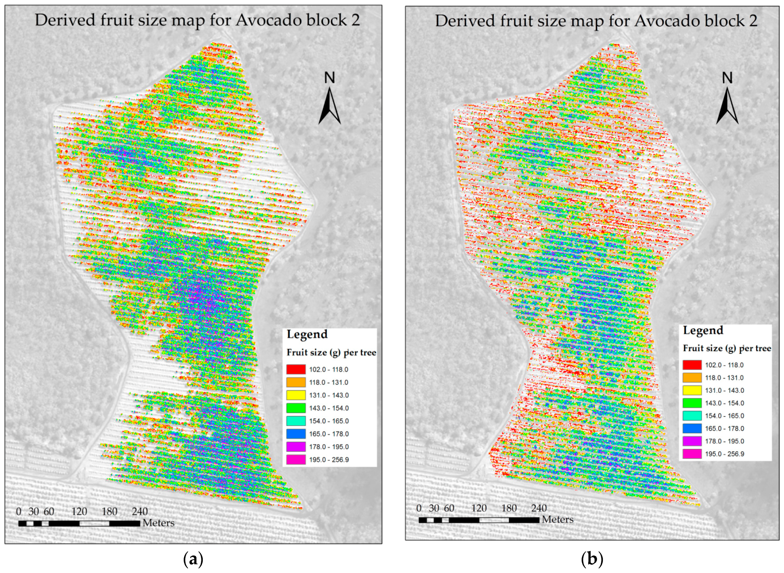
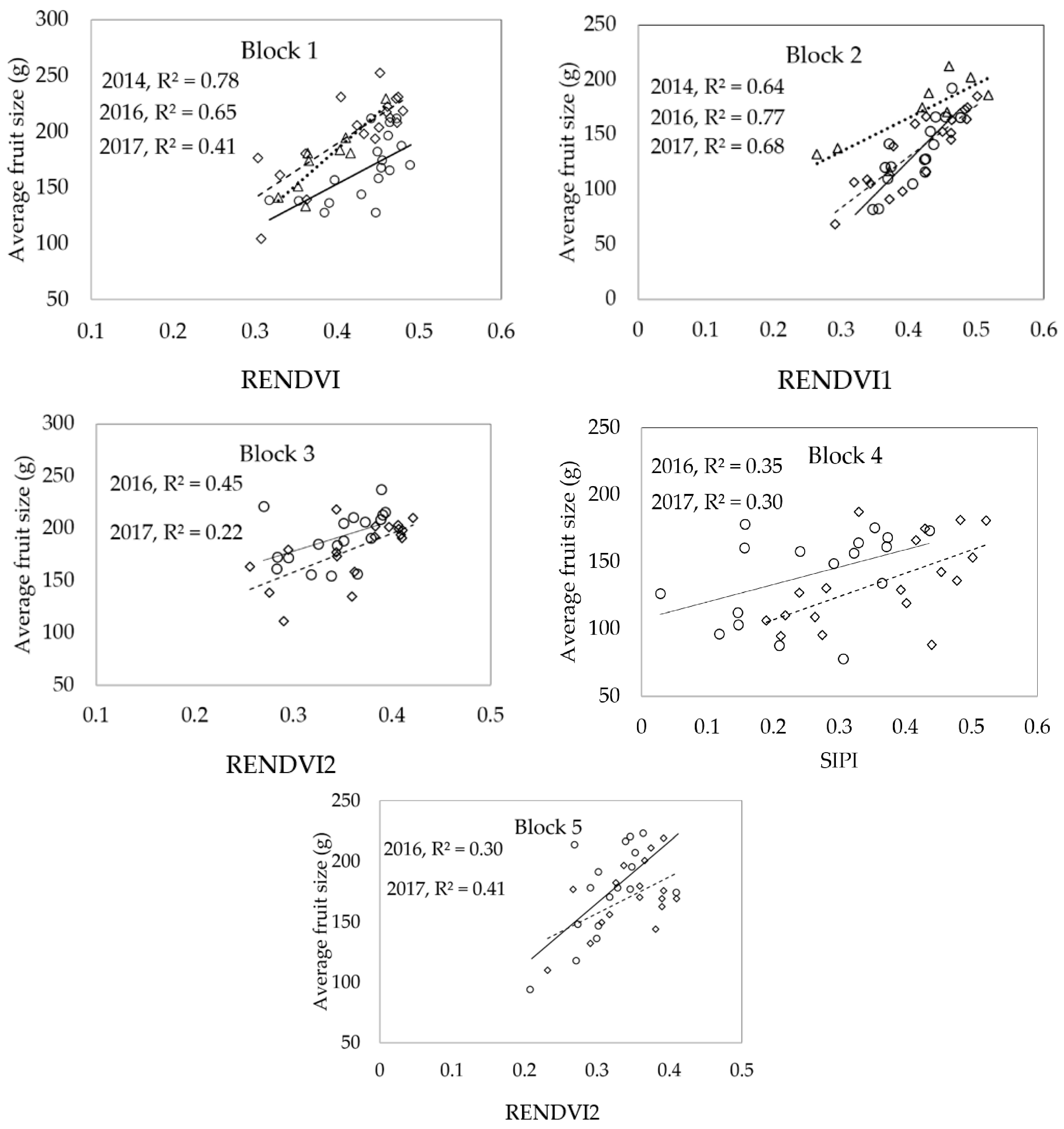
For average fruit size (g), scatter plots of the optimal VIs were again derived for each separate block (Figure 6). Unlike total fruit weight (kg·tree−1), strong coefficients of determination were achieved across all three seasons for Block 1 (RENDVI1: R2 = 0.78 with RMSE = 13 g (2014), R2 = 0.65 with RMSE = 24.8 g (2016) and R2 = 0.41 with RMSE = 43.7 g (2017)) and Block 2 (RENDVI1: R2 = 0.64 with RMSE = 18.78 g (2014), R2 = 0.77 with RMSE = 15.83 g (2016) and R2 = 0.68 with RMSE = 33.5 g (2017)). For the remaining blocks sampled during the 2016 and 2017 growing season, a respectable coefficient of determination were also identified: Block 3 (RENDVI2, R2 = 0.45 with RMSE = 20.96 g); Block 5 (RENDVI2, R2 = 0.41 with RMSE = 43.32 g) and Block 4 (SIPI, R2 = 0.35 with RMSE 88.98 g).
The results of stepwise regression and ANCOVA for average fruit size (g) per tree in all five blocks are shown in Table 3. No significant differences were observed in slopes for any of the three years data for all five blocks, with the lowest p-value = 0.07 for Block 2. However, the intercepts again differed for all blocks except block 5 (F-value = 0.67 and p-value = 0.42). This results show the consistency of correlation between average fruit size (g) per tree data against optimal VI in different years.
3.3. Accuracy of Block Level Yield Maps
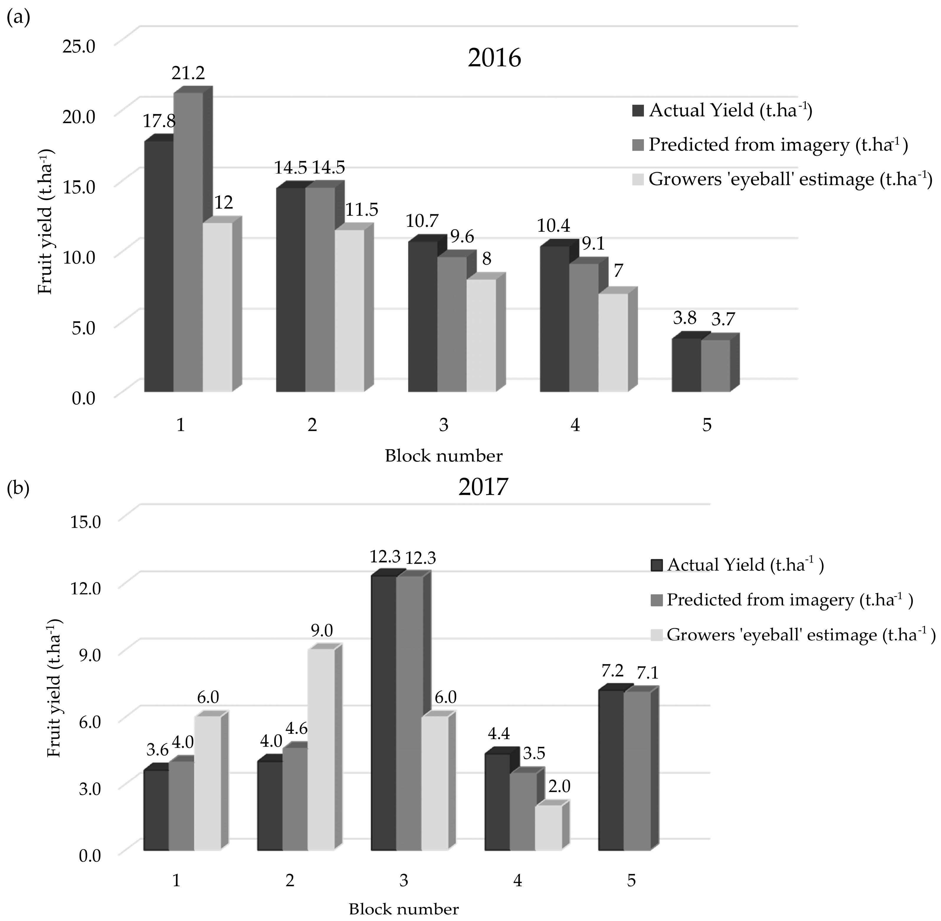
In order to extrapolate the measured yield of the selected trees to the entire orchard block, the process described in Figure 3 was employed for the 2016 and 2017 harvest seasons. Estimations of total fruit weight (t·ha−1) per block were compared against actual commercially harvested yield as well as to grower ‘eye ball’ estimates (Figure 7). The results demonstrate that for all blocks the predicted yield derived from the remotely sensed imagery calibrated with the sampling of strategically located trees, was much closer to actual yield than that provided by the growers ‘eye ball’ estimate. Note, the growers estimated result for Block 5 was not undertaken. The estimation accuracies ranged from an under estimation of 20% (Block 4, 2017) to an over estimation of 19% (Block 1, 2016). The average estimation accuracy for all five blocks was 98.2% in 2016 and 99.5% in 2017.
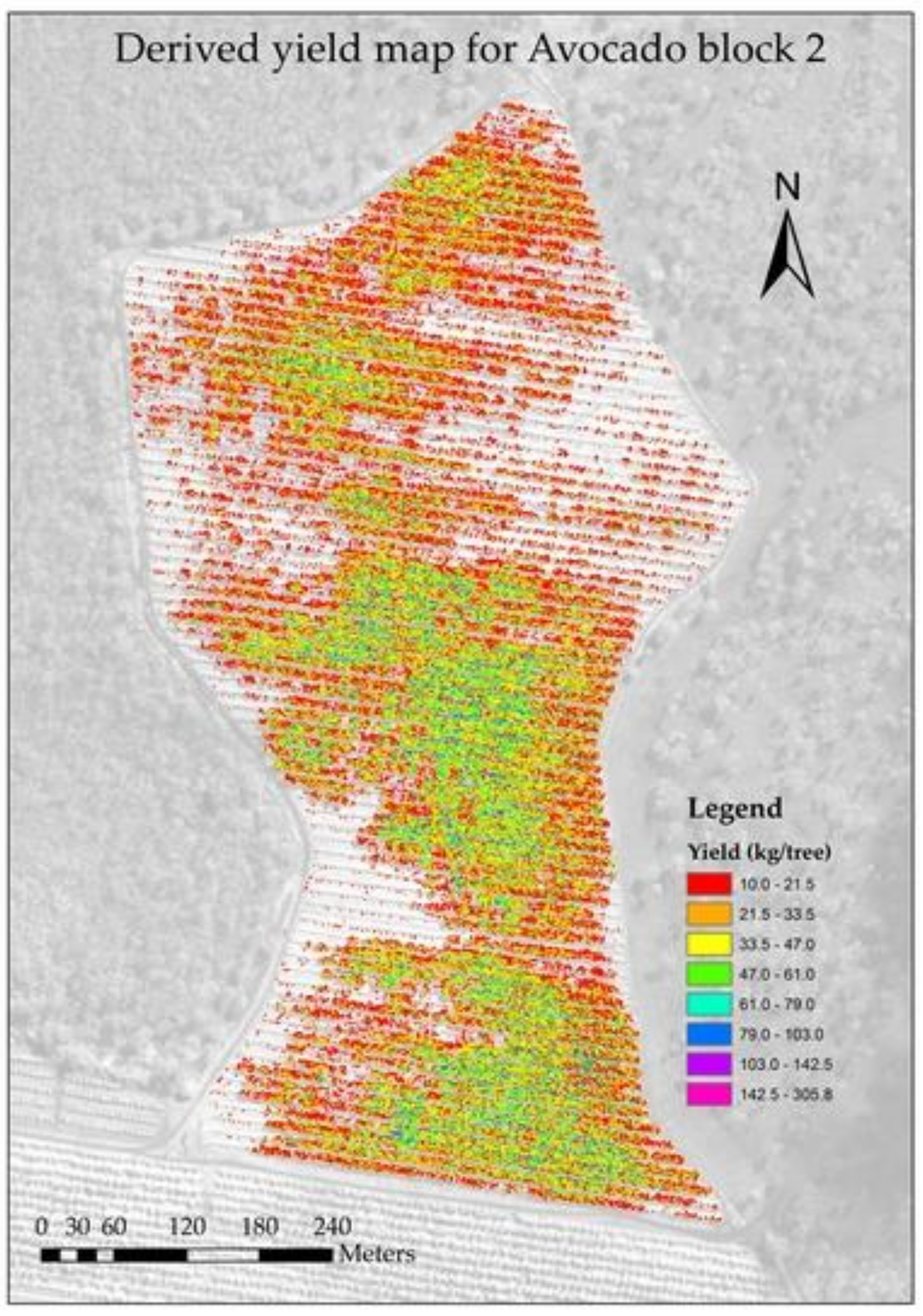
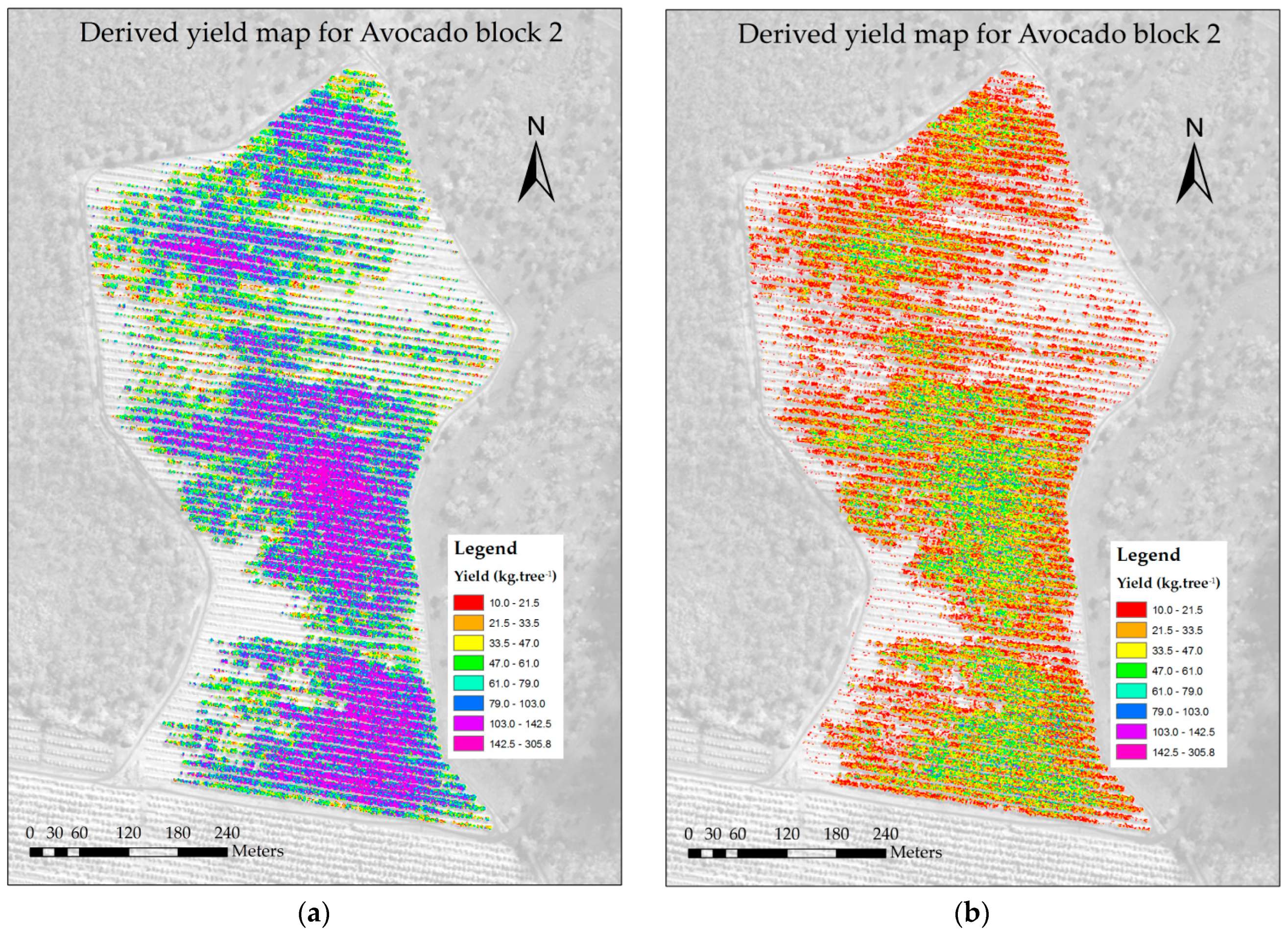
Using the relationship developed with the VIs, yield maps (kg·tree−1) were derived for each block using the process presented in Figure 3. The yield maps of Block 2 in 2016 and 2017 are shown as an example in Figure 8. Maps of average fruit size (g) per tree were also derived for each block, with the maps of Block 2 for the 2016 and 2017 harvest season presented in Figure 9.
4. Discussion
The results from this study indicate the potential of high resolution WV imagery for accurately mapping fruit yield (kg·tree−1) and average fruit size (g) across multiple avocado orchards and seasons in the Bundaberg region of Queensland, Australia. The low R-squared values achieved using the data for all blocks and all years for both yield parameters, and the subsequent increase in R-squared values when the data for each block was analysed separately, suggests that there is not a consistent relationship across all blocks between yield and canopy reflectance as measured by the selected VI. The results suggest that a single ‘generic’ algorithm is not suitable, and that a site specific algorithm (i.e., for each block) is needed to estimate the yield parameters at the individual block level, a result that is consistent with those presented for apple and pear crops [55]. It is likely that climatic factors based on location as well as other factors such as tree age, orchard management (pruning, irrigation and fertiliser or mulch use), soil type, and pollinators are influencing the yield achieved for each block as well as the relationship between canopy reflectance and yield. Furthermore, the relationships between yield and VIs are different for each growing season for each block. This shows the importance of using targeted field sampling during each growing season to calibrate the relationship between yield and the VIs derived from the satellite imagery.
The vegetation indices RENDVI1 and RENDVI2 consistently produced the strongest relationship to the measured yield parameters. This result indicates that variations in the avocado canopy that are sensitive to fruit filling and holding capacity are measurable with the NIR1, NIR2, and Red-edge spectral bands. The Red-edge spectral band has been identified to be highly sensitive to the foliar nitrogen concentration, a plant constituent that is essential for yield development in avocado [56]. Similarly canopy reflectance measures in the NIR1 and NIR2 spectral bands have been related to variations in canopy structure, density and turgidity [4,17]. Therefore, it follows that an avocado canopy that produces lower reflectance in the NIR bands is likely to have lower biomass and potentially lower turgidity, both symptoms of an unhealthy plant. Research has shown that stressed avocado trees are more susceptible to yield decline or smaller fruit than a healthy tree. As an example, trees suffering from constraints such as water stress or Phytophthora (Phytophthora cinnamomi) root rot will produce smaller fruit than a healthy tree [57,58].
The results from the ANCOVA analysis show the consistency of correlation between average fruit size and the optimal VI across different years. While there was no significant difference in p-values for the model slopes (so the relationship remained constant), the significant differences in p-values (p < 0.05) for the model intercepts show that between years the average fruit size achievable differed i.e., in some years average fruit size achievable was higher, possibly due to abiotic or biotic factors such as climate or management.
Prediction of average orchard yield derived from this method, was found to be consistently more accurate than the ‘eyeball’ forecasting method currently adopted by the avocado industry. This has important implications as having accurate pre-harvest yield estimates is important for planning and forward selling. It suggests that the use of the method presented in this study would provide growers with more accurate yield forecasts than the method currently used across the avocado industry.
The block level yield maps of total fruit weight and average fruit size offer significant benefit to growers for harvest segregation at the start of the season when prices for large fruit is optimal. Growers can use this information to better target orchard zones with larger fruit thus saving on labour costs and time currently used for the selective harvesting of every tree. Moreover, the classified maps of total yield (kg·ha−1) and the average fruit size (g) per tree, generated in this study allow growers to visually assess the spatial variation of yield across their blocks, thus enabling them to identify low performing regions. By employing targeted inspections, soil and leaf tissue testing etc., growers can identify the causal constraint and therefore investigate methods of remediation to maximise productivity. In addition, the maps can be used to detect change in fruit yield between years. For example, Figure 9 shows a clearly visible decline in overall yield in 2017, compared to 2016, potentially due to the biennial bearing pattern of avocados.
In this study, a correlation between spectral reflectance derived VIs from WV satellite imagery and both total fruit weight and average fruit size per tree was observed. This result has also been reported in previous studies [4]. Worldview satellite imagery offers high spatial resolution, and individual avocado tree canopies are able to be observed at tree maturity. However, it is also costly to purchase, and a minimum area of 100 m2 is required to be ordered for tasking to occur. Freely available alternatives are Landsat and Sentinel 2 (25 m and 10–20 m pixel resolution respectively). However, the coarser resolution of these satellite images mean that multiple tree canopies determine the spectral reflectance of each pixel. In addition, the red-edge band in WV imagery was shown in this study to be an important predictor of yield and this band is not available from Landsat, and only available at 20 m resolution from Sentinel 2. Other alternatives for imagery capture are unmanned aerial vehicles (UAVs) or manned aircraft. These alternatives are generally more expensive on a cost to area ratio, unless the vehicle and image processing is completed by the orchard grower themselves (something that is beyond the scope of many growers).
For this reason, the purchase of high-resolution satellite imagery such as Worldview is a viable cost-effective solution for orchard variability mapping and yield prediction, particularly if costs are shared between adjacent orchards. It is also possible that new additions such as Planet’s Dove satellites, which offer almost daily temporal coverage, will offer a viable cost-affordable option in terms of spatial resolution (3 m pixels). However, these sensors do not currently provide a re-edge sensor. Further research would need to be completed to determine if the increased temporal frequency offered by the Dove satellite constellation is able to be used for accurate avocado yield prediction.
This study only explored the relationship between yield and satellite imagery in the Bundaberg region of Queenlsand, Australia. It is likely that different relationships will occur in other regions and different VIs to those identified here may be the best predictors of yield. Further research will investigate how VIs relate to avocado yield in other growing regions of Australia.
5. Conclusions
The results from this three-year study indicate that high-resolution multispectral satellite imagery (WV2 and WV3) coupled with targeted field sampling can be used to accurately determine the spatial variability of yield (kg·tree−1) and average fruit size (g) per tree across an avocado orchard. Although, the relationship between canopy reflectance properties (VIs) with total fruit yield (kg·tree−1) was largely variable, the positive relationship to fruit size (g) per tree remained consistent. This result, offers great benefit to avocado growers as the largest fruit can be better located and then selectively harvested at the start of the season when prices are high. This offers efficiencies in time, fuel costs and labour. In terms of yield, the estimation accuracies achieved from satellite imagery for all five blocks in 2016 and 2017 far exceeded those derived from the ‘eyeball’ method of yield estimation. Although RENDVI1 was identified as the best algorithm for yield estimation across all blocks, the relatively low coefficient of determination indicated growing location and season were influencing the relationship. To further assess the robustness of this methodology, additional growing locations and growing years with different varieties are warranted.
Acknowledgments
The authors of this paper would like to acknowledge the Federal Government–funded Rural Research and Development for Profit Scheme and Horticulture Innovation Australia Ltd. for funding this research, as well as Avocado Australia Ltd. for their support. Also, Chad Simpson (Simpson Farms), David Depaoli (Auschilli), and Tom Redfern for their collaboration with this research. Derek Schneider, Lucinda Frizell, Ashley Saint, and Bryony Wilcox (University of New England) and Jonathon Smith (Department of Agriculture and Fisheries Queensland) for assistance with in-field sampling.
Author Contributions
Andrew Robson conceived and designed the experiments; Andrew Robson, Muhammad Moshiur Rahman, and Jasmine Muir analysed the data and wrote the paper.
Conflicts of Interest
The authors declare no conflict of interest.
References
- Papageorgiou, E.I.; Aggelopoulou, K.D.; Gemtos, T.A.; Nanos, G.D. Yield prediction in apples using Fuzzy Cognitive Map learning approach. Comput. Electron. Agric. 2013, 91, 19–29. [Google Scholar] [CrossRef]
- Wang, Q.; Nuske, S.; Bergerman, M.; Singh, S. Automated Crop Yield Estimation for Apple Orchards. In Experimental Robotics: The 13th International Symposium on Experimental Robotics; Desai, P.J., Dudek, G., Khatib, O., Kumar, V., Eds.; Springer International Publishing: Heidelberg, Germany, 2013; pp. 745–758. [Google Scholar]
- Köhne, S. Yield estimation based on measureable parameters. S. Afr. Avocado Grow. Assoc. Yearb. 1985, 8, 103:1–103:3. [Google Scholar]
- Robson, A.J.; Petty, J.; Joyce, D.C.; Marques, J.R.; Hofman, P.J. High resolution remote sensing, GIS and Google Earth for avocado fruit quality mapping and tree number auditing. In Proceedings of the 29th International Horticultural Congress, Brisbane Convention and Exhibition Centre, Brisbane, Australia, 17–22 August 2014; pp. 589–595. [Google Scholar]
- Zamora, F.A.; Téllez, C.P.; Wulfsohn, D.; Zamora, I.; García-Fiñana, M. Performance of a procedure for fruit yield estimation. In Proceedings of the American Society of Agricultural and Biological Engineers Annual International Meeting, Pittsburgh, PA, USA, 20–23 June 2010; pp. 5275–5290. [Google Scholar]
- Winter, F. A Simulation Model for Studying the Efficiency of Apple and Pear Orchards/Ein Simulationsmodell zur Untersuchung der Wirtschaftlichkeit von Apfel-und Birnenanlagen. Gartenbauwissenschaft 1976, 14, 26–34. [Google Scholar]
- Aggelopoulou, K.D.; Wulfsohn, D.; Fountas, S.; Gemtos, T.A.; Nanos, G.D.; Blackmore, S. Spatial variation in yield and quality in a small apple orchard. Precis. Agric. 2010, 11, 538–556. [Google Scholar] [CrossRef]
- Alburquerque, N.; Burgos, L.; Egea, J. Influence of flower bud density, flower bud drop and fruit set on apricot productivity. Sci. Hortic. 2004, 102, 397–406. [Google Scholar] [CrossRef]
- Whiley, A.W.; Saranah, J.B.; Rasmussen, T.S. The Relationship between Carbohydrate Levels and Productivity in the Avocado and Impact on Management Practices, Particularly Time of Harvest; Horticultural Research and Development Corporation: Gordon, Australia, 1996.
- Zaman, Q.; Schumann, A.; Percival, D.; Gordon, R. Estimation of wild blueberry fruit yield using digital color photography. Trans. ASABE 2008, 51, 1539–1544. [Google Scholar] [CrossRef]
- Zhou, R.; Damerow, L.; Sun, Y.; Blanke, M.M. Using colour features of cv. ‘Gala’ apple fruits in an orchard in image processing to predict yield. Precis. Agric. 2012, 13, 568–580. [Google Scholar] [CrossRef]
- Annamalai, P.; Lee, W.S.; Burks, T. Color Vision Systems for Estimating Citrus Yield in Real-Time; ASAE Paper No. 040354; ASAE: St. Joseph, MI, USA, 2004. [Google Scholar]
- Bulanon, D.M.; Kataoka, T.; Ota, Y.; Hiroma, T. AE—Automation and Emerging Technologies. Biosyst. Eng. 2002, 83, 405–412. [Google Scholar] [CrossRef]
- Lee, W.S. Citrus Yield Mapping System in Natural Outdoor Scenes using the Watershed Transform. In Proceedings of the 2006 ASABE Annual International Meeting Sponsored, ASABE Oregon Convention Center, Portland, OR, USA, 9–12 July 2006. [Google Scholar]
- Stajnko, D.; Lakota, M.; Hočevar, M. Estimation of number and diameter of apple fruits in an orchard during the growing season by thermal imaging. Comput. Electron. Agric. 2004, 42, 31–42. [Google Scholar] [CrossRef]
- Doraiswamy, P.C.; Moulin, S.; Cook, P.W.; Stern, A. Crop yield assessment from remote sensing. Photogramm. Eng. Remote Sens. 2003, 69, 665–674. [Google Scholar] [CrossRef]
- Prasad, A.K.; Chai, L.; Singh, R.P.; Kafatos, M. Crop yield estimation model for Iowa using remote sensing and surface parameters. Int. J. Appl. Earth Obs. Geoinf. 2006, 8, 26–33. [Google Scholar] [CrossRef]
- Shanahan, J.F.; Schepers, J.S.; Francis, D.D.; Varvel, G.E.; Wilhelm, W.W.; Tringe, J.M.; Schlemmer, M.R.; Major, D.J. Use of Remote-Sensing Imagery to Estimate Corn Grain Yield. Agron. J. 2001, 93, 583–589. [Google Scholar] [CrossRef]
- Rahman, M.M.; Robson, A.J. A Novel Approach for Sugarcane Yield Prediction Using Landsat Time Series Imagery: A Case Study on Bundaberg Region. Adv. Remote Sens. 2016, 5, 93–102. [Google Scholar] [CrossRef]
- Robson, A.J. Remote Sensing Applications for the Determination of Yield, Maturity and Aflatoxin Contamination in Peanut. Ph.D. Thesis, University of Queensland, St. Lucia, Australia, 2007. [Google Scholar]
- Rembold, F.; Atzberger, C.; Savin, I.; Rojas, O. Using Low Resolution Satellite Imagery for Yield Prediction and Yield Anomaly Detection. Remote Sens. 2013, 5, 1704–1733. [Google Scholar] [CrossRef] [Green Version]
- Zhang, X.; Chen, S.; Sun, H.; Pei, D.; Wang, Y. Dry matter, harvest index, grain yield and water use efficiency as affected by water supply in winter wheat. Irrig. Sci. 2008, 27, 1–10. [Google Scholar] [CrossRef]
- Cannell, M.G.R. Dry matter partitioning in tree crops. In Attributes of Trees as Crop Plants; Cannell, M.G.R., Jackson, J.E., Eds.; Institute of Terrestrial Ecology: Abbotts Ripton, UK, 1985; pp. 160–193. [Google Scholar]
- Somers, B.; Delalieux, S.; Verstraeten, W.; Vanden Eynde, A.; Barry, G.; Coppin, P. The contribution of the fruit component to the hyperspectral citrus canopy signal. Photogramm. Eng. Remote Sens. 2010, 76, 37–47. [Google Scholar] [CrossRef]
- Ye, X.; Sakai, K.; Manago, M.; Asada, S.-I.; Sasao, A. Prediction of citrus yield from airborne hyperspectral imagery. Precis. Agric. 2007, 8, 111–125. [Google Scholar] [CrossRef]
- Best, S.; Salazar, F.; Bastias, R.; Leon, L. Crop-load estimation model to optimize yield-Quality ratio in apple orchards, Malus Domestic Borkh, var. Royal Gala. J. Inf. Technol. Agric. 2008, 3, 11–18. [Google Scholar]
- Van Beek, J.; Tits, L.; Somers, B.; Deckers, T.; Verjans, W.; Bylemans, D.; Janssens, P.; Coppin, P. Temporal Dependency of Yield and Quality Estimation through Spectral Vegetation Indices in Pear Orchards. Remote Sens. 2015, 7, 9886–9903. [Google Scholar] [CrossRef]
- Sepulcre-Cantó, G.; Zarco-Tejada, P.J.; Jiménez-Muñoz, J.C.; Sobrino, J.A.; Soriano, M.A.; Fereres, E.; Vega, V.; Pastor, M. Monitoring yield and fruit quality parameters in open-canopy tree crops under water stress. Implications for ASTER. Remote Sens. Environ. 2007, 107, 455–470. [Google Scholar] [CrossRef]
- Payne, A.B.; Walsh, K.B.; Subedi, P.P.; Jarvis, D. Estimation of mango crop yield using image analysis—Segmentation method. Comput. Electron. Agric. 2013, 91, 57–64. [Google Scholar] [CrossRef]
- Serrano, L.; González-Flor, C.; Gorchs, G. Assessment of grape yield and composition using the reflectance based Water Index in Mediterranean rainfed vineyards. Remote Sens. Environ. 2012, 118, 249–258. [Google Scholar] [CrossRef] [Green Version]
- Hall, A.; Lamb, D.W.; Holzapfel, B.; Louis, J. Optical remote sensing applications in viticulture—A review. Aust. J. Grape Wine Res. 2002, 8, 36–47. [Google Scholar] [CrossRef]
- Jensen, J.R. Remote Sensing of the Environment: An Earth Resources Perspective; Prentice-Hall: Upper Saddle River, NJ, USA, 2000. [Google Scholar]
- Rouse, J.W.; Haas, R.H.; Schell, J.A.; Deering, D.W. Monitoring vegetation systems in the Great Plains with ERTS. In Proceedings of the Third Earth Resources Technology Satellite-1 Symposium—Volume I: Technical Presentations; NASA SP-351; NASA: Washington, DC, USA, 1974; pp. 309–317. [Google Scholar]
- Jordan, C.F. Derivation of Leaf-Area Index from Quality of Light on the Forest Floor. Ecology 1969, 50, 663–666. [Google Scholar] [CrossRef]
- Apan, A.; Held, A.; Phinn, S.; Markley, J. Formulation and assessment of narrow-band vegetation indices from EO-1 Hyperion imagery for discriminating sugarcane disease. In Proceedings of the Spatial Sciences Institute Biennial Conference (SSC 2003): Spatial Knowledge Without Boundaries, Canberra, Australia, 22–26 September 2003. [Google Scholar]
- Maitra, S.; Yan, J. Principle component analysis and partial least squares: Two dimension reduction techniques for regression. Appl. Multivar. Stat. Models 2008, 79, 79–90. [Google Scholar]
- Tobias, R.D. An introduction to partial least squares regression. In Proceedings of the Twentieth Annual SAS Users Group International Conference; SAS: Cary, NC, USA, 1995; pp. 1250–1257. [Google Scholar]
- BOM. Bureau of Meteorology. Available online: http://www.bom.gov.au (accessed on 7 July 2017).
- Newett, S.; Whiley, A.; Dirou, J.; Hofman, P.; Ireland, G.; Kernot, L.; Ledger, S.; McCarthy, A.; Miller, J.; Pinese, B.; et al. Avocado Information Kit; Agrilink Series QAL9906; Department of Primary Industries: Taabinga, Australia, 2001.
- Whiley, A.; Hargreaves, P.; Pegg, K.; Doogan, V.; Ruddle, L.; Saranah, J.; Langdon, P. Changing sink strengths influence translocation of phosphonate in avocado (Persea americana Mill.) trees. Aust. J. Agric. Res. 1995, 46, 1079–1090. [Google Scholar] [CrossRef]
- Kuester, M. Radiometric Use of WorldView-3 Imagery; DigitalGlobe: Longmont, CO, USA, 2016. [Google Scholar]
- Rueda, C.A.; Greenberg, J.A.; Ustin, S.L. StarSpan: A Tool for Fast Selective Pixel Extraction from Remotely Sensed Data; Center for Spatial Technologies and Remote Sensing (CSTARS), University of California at Davis: Davis, CA, USA, 2005. [Google Scholar]
- Gobron, N.; Pinty, B.; Verstraete, M.M.; Widlowski, J.-L. Advanced vegetation indices optimized for up-coming sensors: Design, performance, and applications. IEEE Trans. Geosci. Remote Sens. 2000, 38, 2489–2505. [Google Scholar]
- Haboudane, D.; Miller, J.R.; Tremblay, N.; Zarco-Tejada, P.J.; Dextraze, L. Integrated narrow-band vegetation indices for prediction of crop chlorophyll content for application to precision agriculture. Remote Sens. Environ. 2002, 81, 416–426. [Google Scholar] [CrossRef]
- Penuelas, J.; Baret, F.; Filella, I. Semi-empirical indices to assess carotenoids/chlorophyll a ratio from leaf spectral reflectance. Photosynthetica 1995, 31, 221–230. [Google Scholar]
- Gitelson, A.A.; Merzlyak, M.N.; Lichtenthaler, H.K. Detection of Red Edge Position and Chlorophyll Content by Reflectance Measurements Near 700 nm. J. Plant Physiol. 1996, 148, 501–508. [Google Scholar] [CrossRef]
- Gitelson, A.A.; Kaufman, Y.J.; Merzlyak, M.N. Use of a green channel in remote sensing of global vegetation from EOS-MODIS. Remote Sens. Environ. 1996, 58, 289–298. [Google Scholar] [CrossRef]
- Chen, J.M. Evaluation of vegetation indices and a modified simple ratio for boreal applications. Can. J. Remote Sens. 1996, 22, 229–242. [Google Scholar] [CrossRef]
- Fitzgerald, G.; Rodriguez, D.; O’Leary, G. Measuring and predicting canopy nitrogen nutrition in wheat using a spectral index—The canopy chlorophyll content index (CCCI). Field Crop. Res. 2010, 116, 318–324. [Google Scholar] [CrossRef]
- Pu, R.; Landry, S. A comparative analysis of high spatial resolution IKONOS and WorldView-2 imagery for mapping urban tree species. Remote Sens. Environ. 2012, 124, 516–533. [Google Scholar] [CrossRef]
- Roujean, J.-L.; Breon, F.-M. Estimating PAR absorbed by vegetation from bidirectional reflectance measurements. Remote Sens. Environ. 1995, 51, 375–384. [Google Scholar] [CrossRef]
- Bannari, A.; Asalhi, H.; Teillet, P.M. Transformed difference vegetation index (TDVI) for vegetation cover mapping. In Proceedings of the 2002 IEEE International Conference on Geoscience and Remote Sensing Symposium, Toronto, ON, Canada, 24–28 June 2002; Volume 3055, pp. 3053–3055. [Google Scholar]
- Goel, N.S.; Qin, W. Influences of canopy architecture on relationships between various vegetation indices and LAI and FPAR: A computer simulation. Remote Sens. Rev. 1994, 10, 309–347. [Google Scholar] [CrossRef]
- R Development Core Team. R: A Language and Environment for Statistical Computing (Version 3.3.3); R Foundation for Statistical Computing: Vienna, Austria, 2017. [Google Scholar]
- Lötze, E.; Bergh, O. Early prediction of harvest fruit size distribution of an apple and pear cultivar. Sci. Hortic. 2004, 101, 281–290. [Google Scholar] [CrossRef]
- Whiley, A.W.; Saranah, J.B.; Wolstenholme, B.N. Pheno-physiological modelling in avocado—An aid in research planning. In Proceedings of the World Avocado Congress III, Tel Aviv, Israel, 22–27 October 1995; pp. 71–75. [Google Scholar]
- Curran, P.J.; Windham, W.R.; Gholz, H.L. Exploring the relationship between reflectance red edge and chlorophyll concentration in slash pine leaves. Tree Physiol. 1995, 15, 203–206. [Google Scholar] [CrossRef] [PubMed]
- Schaffer, B.A.; Wolstenholme, B.N.; Whiley, A.W. The Avocado: Botany, Production and Uses; CABI: Wallingford, UK, 2013. [Google Scholar]
Figure 1.
Location of the five avocado orchards in Bundaberg, Queensland, Australia (green polygons).
Figure 1.
Location of the five avocado orchards in Bundaberg, Queensland, Australia (green polygons).
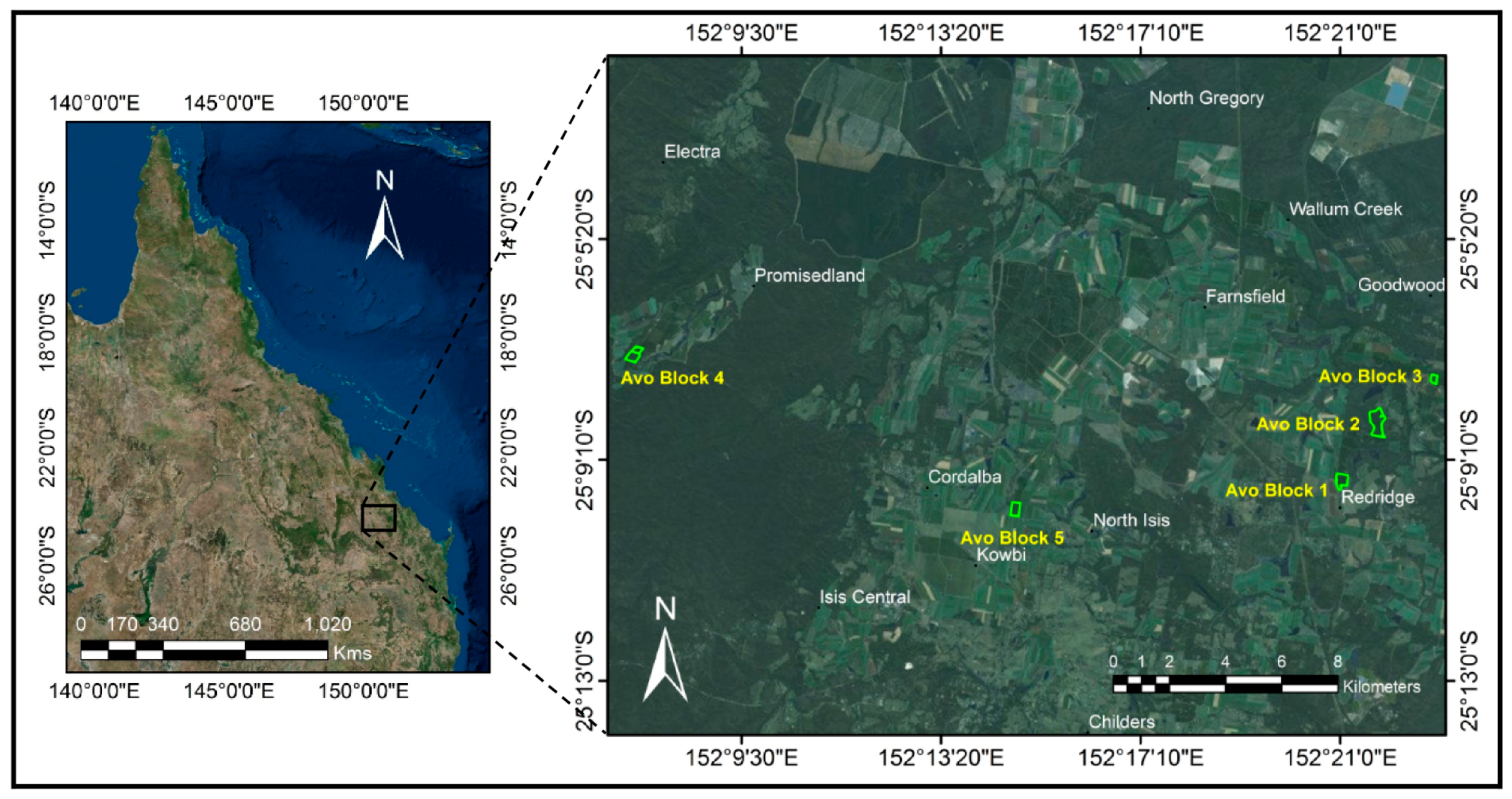
Figure 2.
Classified Normalised Difference Vegetation Index (NDVI) images of the five avocado blocks with sampling locations for the 2016 and 2017 season presented as black circles. In Block 1 and 2, the individual tree sampling locations for 2014 are indicated as white circles. (Note some sample locations overlap between years.) Block 1: 14.4 ha, Block 2: 28.2 ha, Block 3: 6.8 ha, Block 4: 14.7 ha, Block 5: 12.7 ha and Block 6: 11.3 ha.

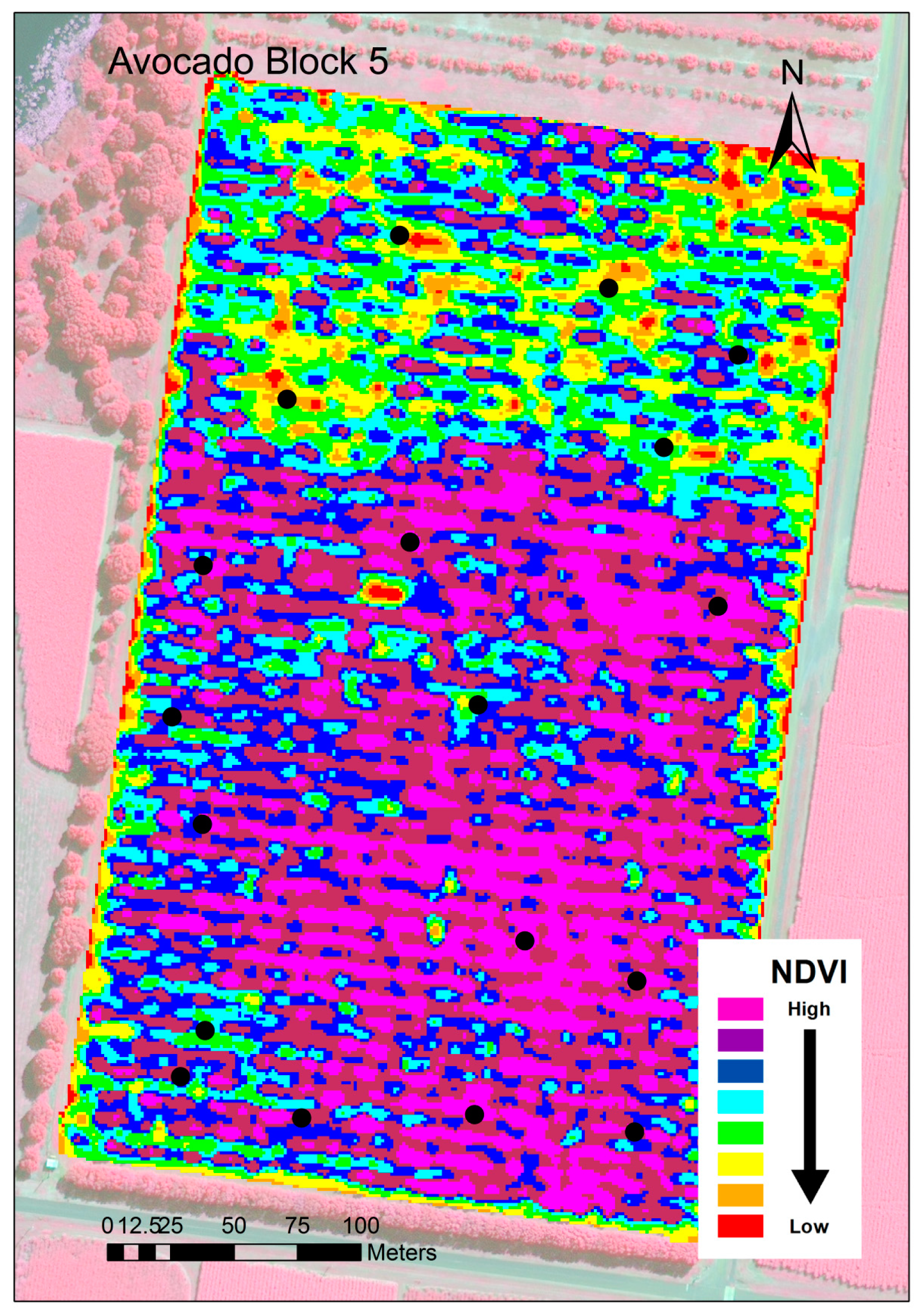
Figure 3.
Process of deriving parameter specific map from WorldView-3 (WV3) imagery using the algorithm developed from the 18 sampled trees per block.
Figure 3.
Process of deriving parameter specific map from WorldView-3 (WV3) imagery using the algorithm developed from the 18 sampled trees per block.

Figure 4.
Scatter plot between the red edge band (RENDVI1) VI identified to have the highest coefficient of determination across all blocks for (a) total fruit weight (kg·tree−1) and (b) average fruit size (g) per tree. The 2014 sample points are presented as a triangle (∆) (n = 18) with dotted best fit line, the 2016 as a diamond (◊) (n = 18) with dashed best fit line, and the 2017 as a circle (o) (n = 108) with solid best fit line.

Figure 5.
Scatter plot between those VIs identified to have the highest coefficient of determination to total fruit weight (kg·tree−1) for each sampled block derived from WorldView-2 (WV2) and WV3 imagery. The 2014 sample points are presented as a triangle (∆) (n = 9 per block) in blocks 1 and 2, with 2016 as a diamond (◊) (n = 18 per block) and 2017 as circle (o) (n = 18 per block).

Figure 6.
Scatter plot between those VIs identified to have the highest coefficient of determination to average fruit weight per tree (g) for each sampled block derived from WV2 and WV3 imagery. The 2014 sample points are presented as a triangle (∆) (n = 9 per block) in blocks 1 and 2, with 2016 as a diamond (◊) (n = 18 per block) and 2017 as circle (o) (n = 18 per block).

Figure 7.
Comparison between the actual yield (t·ha−1) to that predicted from satellite imagery and that made by visual assessment from growers in (a) 2016 and (b) 2017. Note that no growers estimate was supplied for Block 5.
Figure 7.
Comparison between the actual yield (t·ha−1) to that predicted from satellite imagery and that made by visual assessment from growers in (a) 2016 and (b) 2017. Note that no growers estimate was supplied for Block 5.

Figure 8.
Classified yield maps derived from the best fit model of the relationship between VIs and total fruit weight (kg·tree−1) for Block 2 in (a) 2016 and (b) 2017.
Figure 8.
Classified yield maps derived from the best fit model of the relationship between VIs and total fruit weight (kg·tree−1) for Block 2 in (a) 2016 and (b) 2017.

Figure 9.
Classified fruit size (g) per tree maps derived from the best fit model of the relationship between VIs and average fruit size (g) per tree for Block 2 in (a) 2016 and (b) 2017.
Figure 9.
Classified fruit size (g) per tree maps derived from the best fit model of the relationship between VIs and average fruit size (g) per tree for Block 2 in (a) 2016 and (b) 2017.

Table 1.
Vegetation indices used in this study.
| NAME | FORMULA | REFERENCES | |
|---|---|---|---|
| 1 | Normalized Difference Rededge/Red (NDVI rededge) | (RE − R)/(RE + R) | [43] |
| 2 | Transformed Chlorophyll Absorption in Reflectance Index (TCARI) | 3 × ((RE − R) − 0.2 × (RE − G) × (RE/R)) | [44] |
| 3 | Structure Insensitive Pigment Index (SIPI) | (NIR1 − B)/(NIR1 + R) | [45] |
| 4 | Coastal Blue Structure Insensitive Pigment Index (CB SIPI) | (NIR1 − CB)/(NIR1 + CB) | [45] |
| 5 | Normalized difference Red/Red-edge index (R/RENDVI) | (NIR1 − R)/(NIR1 + RE) | [46] |
| 6 | Normalized difference Red/NIR2 index (R/N2NDVI) | (NIR1 − R)/(NIR1 + NIR2) | [4] |
| 7 | Green normalized difference vegetation index (GNDVI) | (NIR1 − G)/(NIR1 + G) | [47] |
| 8 | Modified Simple Ratio (MSR) | (NIR1/R − 1)/(SQRT((NIR1/R) + 1)) | [48] |
| 9 | Ratio Vegetation Index (RVI) | NIR1/R | [34] |
| 10 | Normalized Difference Vegetation Index (N1NDVI) | (NIR1 − R)/(NIR1 + R) | [33] |
| 11 | Normalized Difference Vegetation Index (N2NDVI) | (NIR2 − R)/(NIR2 + R) | [33] |
| 12 | Normalized difference red edge index 1 (RENDVI1) | (NIR1 − RE)/(NIR1 + RE) | [49] |
| 13 | Normalized difference red edge index 2 (RENDVI2) | (NIR2 − RE)/(NIR2 + RE) | [50] |
| 14 | RDVI1 | (NIR1 − R)/(SQRT (NIR1 + R)) | [51] |
| 15 | RDVI2 | (NIR2 − R)/(SQRT (NIR2 + R)) | [51] |
| 16 | Transformed difference vegetation index (TDVI) | 1.5 × ((NIR1 − R)/(SQRT(NIR12 + R + 0.5)) | [52] |
| 17 | Transformed difference vegetation index 2 (TDVI2) | 1.5 × ((NIR2 − R)/(SQRT(NIR22 + R + 0.5)) | [52] |
| 18 | Non Linear Index (NLI) | (NIR2 − R)/(NIR2 + R) | [53] |
Table 2.
Best vegetation indices (VIs) for all blocks and for each block for average fruit size (g) per tree and total fruit weight (kg·tree−1) using principal component analysis (PCA) and non-linear regression.
Table 2.
Best vegetation indices (VIs) for all blocks and for each block for average fruit size (g) per tree and total fruit weight (kg·tree−1) using principal component analysis (PCA) and non-linear regression.
| Blocks | Total Fruit Weight (kg·tree−1) | Average Fruit Size (g) Per Tree | ||||
|---|---|---|---|---|---|---|
| PCA | Non-Linear Regression | R2 | PCA | Non-Linear Regression | R2 | |
| All blocks for 3 years | RENDVI1, RENDVI2 | RENDVI1 | 0.29 | RENDVI1, RENDVI2 | RENDVI1 | 0.29 |
| block 1 (3 years) | RENDVI1, N1GNDVI | N1GNDVI | 0.48 | RENDVI1, N1/RENDVI | RENDVI1 | 0.39 |
| Block 2 (3 years) | RENDVI1, RENDVI2 | RENDVI2 | 0.25 | RENDVI1, RENDVI2 | RENDVI1 | 0.43 |
| Block 3 (2 years) | CB SIPI, Yellow SAVI | CB SIPI | 0.40 | RENDVI2, CB SIPI | RENDVI2 | 0.28 |
| Block 4 (2 years) | SIPI, Yellow SAVI | SIPI | 0.43 | Yellow SAVI, RDVI | Yellow SAVI | 0.19 |
| Block 5 (2 years) | RENDVI2, RENDVI1 | RENDVI2 | 0.49 | RENDVI2, RENDVI1 | RENDVI2 | 0.40 |
Table 3.
The stepwise regression and Analysis of covariance (ANCOVA) results for average fruit size (g) per tree for Block 1 and 2 in three years period and Block 3, 4, and 5 in two years period.
Table 3.
The stepwise regression and Analysis of covariance (ANCOVA) results for average fruit size (g) per tree for Block 1 and 2 in three years period and Block 3, 4, and 5 in two years period.
| Blocks | Slopes | Intercepts | ||
|---|---|---|---|---|
| F-Value | p-Value | F-Value | p-Value | |
| Block 1 | 0.72 | 0.49 | 16 | 0 |
| Block 2 | 2.85 | 0.07 | 11.6 | 0.0001 |
| Block 3 | 0.23 | 0.63 | 4.72 | 0.04 |
| Block 4 | 0.23 | 0.63 | 3.98 | 0.05 |
| Block 5 | 2.87 | 0.10 | 0.67 | 0.42 |
© 2017 by the authors. Licensee MDPI, Basel, Switzerland. This article is an open access article distributed under the terms and conditions of the Creative Commons Attribution (CC BY) license (http://creativecommons.org/licenses/by/4.0/).
Share and Cite
MDPI and ACS Style
Robson, A.; Rahman, M.M.; Muir, J. Using Worldview Satellite Imagery to Map Yield in Avocado (Persea americana): A Case Study in Bundaberg, Australia. Remote Sens. 2017, 9, 1223. https://doi.org/10.3390/rs9121223
AMA Style
Robson A, Rahman MM, Muir J. Using Worldview Satellite Imagery to Map Yield in Avocado (Persea americana): A Case Study in Bundaberg, Australia. Remote Sensing. 2017; 9(12):1223. https://doi.org/10.3390/rs9121223
Chicago/Turabian StyleRobson, Andrew, Muhammad Moshiur Rahman, and Jasmine Muir. 2017. "Using Worldview Satellite Imagery to Map Yield in Avocado (Persea americana): A Case Study in Bundaberg, Australia" Remote Sensing 9, no. 12: 1223. https://doi.org/10.3390/rs9121223
Note that from the first issue of 2016, this journal uses article numbers instead of page numbers. See further details here.