Ionosphere Model for European Region Based on Multi-GNSS Data and TPS Interpolation


1
Institute of Geodesy, University of Warmia and Mazury in Olsztyn, 19-719 Olsztyn, Poland
2
Institute of Geodesy and Geoinformatics, Wroclaw University of Environmental and Life Sciences, 50-357 Wroclaw, Poland
*
Author to whom correspondence should be addressed.
Remote Sens. 2017, 9(12), 1221; https://doi.org/10.3390/rs9121221
Submission received: 23 October 2017
/
Revised: 22 November 2017
/
Accepted: 23 November 2017
/
Published: 27 November 2017
(This article belongs to the Special Issue Multi-Constellation Global Navigation Satellite Systems: Methods and Applications)
Abstract
:The ionosphere is still considered one of the most significant error sources in precise Global Navigation Satellite Systems (GNSS) positioning. On the other hand, new satellite signals and data processing methods allow for a continuous increase in the accuracy of the available ionosphere models derived from GNSS observables. Therefore, many research groups around the world are conducting research on the development of precise ionosphere products. This is also reflected in the establishment of several ionosphere-related working groups by the International Association of Geodesy. Whilst a number of available global ionosphere maps exist today, dense regional GNSS networks often offer the possibility of higher accuracy regional solutions. In this contribution, we propose an approach for regional ionosphere modelling based on un-differenced multi-GNSS carrier phase data for total electron content (TEC) estimation, and thin plate splines for TEC interpolation. In addition, we propose a methodology for ionospheric products self-consistency analysis based on calibrated slant TEC. The results of the presented approach are compared to well-established global ionosphere maps during varied ionospheric conditions. The initial results show that the accuracy of our regional ionospheric vertical TEC maps is well below 1 TEC unit, and that it is at least a factor of 2 better than the global products.
1. Introduction
In the last decades, Global Navigation Satellite Systems (GNSS) have been rapidly evolving and have found a large number of applications in a broad range of commercial and scientific fields. Along with the increase in using space geodetic techniques, the need for more accurate and reliable results is growing still. For this purpose, technical improvements minimizing the effects of the error sources are necessary [1]. At the same time, one of the most significant error sources in precise GNSS positioning is still ionospheric delay of the satellite signals [2]. The ionosphere is a layer of the atmosphere ranging from about 50 to 1000 km consisting mostly of ionized particles that cause satellite signals to be delayed or advanced. The magnitude of the ionospheric effects is determined by the amount of ionospheric total electron content (TEC) and the frequency of electromagnetic waves, and varies from 1 m to more than 100 m. This is due to the fact that the ionosphere changes dynamically under the influence of the highly variable sun.
Reliable modeling of the propagation errors in the ionosphere is essential to support carrier phase ambiguity resolution in precise GNSS positioning. This is especially important in the network RTK (real time kinematic) positioning technique, and also static positioning over longer baselines. As has been shown, the ionospheric delay is characterized by spatial correlation decreasing with the increasing distance of a baseline. Therefore, it is difficult to remove the ionospheric effects through data double-differencing (DD) [3,4,5]. Note that static positioning based on longer observing sessions may utilize ionosphere-free (L3) linear combination of L1 and L2 signals. However, L3 carrier phase ambiguities lose their integer nature and cannot be fixed to integers [2].
The precise GNSS positioning requires very accurate ionospheric corrections to support carrier phase ambiguity resolution [6]. This is particularly true for single-frequency solutions. For this purpose, the parameters of the ionosphere, such as TEC, must be modeled. Due to complexity and diversity of ionospheric processes, there are different approaches to ionosphere modelling. The data assimilation models, e.g., the Global Assimilative Ionospheric Model [7], are based on physical properties of the ionosphere. Other empirical models such as the International Reference Ionosphere (IRI) [8] or NeQuick2 [9], are based on statistical analysis of the results of measurements. There are also models that use purely mathematical approaches to estimate the corresponding model parameters, allowing them to be calculated based on data from space geodetic techniques [1]. According to Alizadeh et al. [1], for TEC parameterization in their global and regional solutions, appropriate base functions, such as spherical harmonics (SH) or 2-D B-splines, should be chosen. Several authors have proven that the use of other functions, e.g., kriging or least squares collocation (LSQ) methods, are also possible [10,11,12,13,14]. The LSQ method seems particularly suitable, however for operational use it requires high computing power as it requires computation of the empirical covariance function [14].
The majority of various global, regional and local ionosphere models currently available are characterized by low temporal and spatial resolutions. Most of them are based on carrier phase-smoothed pseudorange data, which presents low accuracy and requires strong smoothing filters. As a result, the obtained ionospheric delay represents relatively low accuracy of several TEC units (1 Total Electron Content Unit = 1 TECU = 1016 el/m2, and it is equivalent to 0.162 m of L1 signal delay). This is one of the reasons why spherical harmonics expansion (SHE) is used for the global and regional TEC parameterization [15,16,17]. The smoothing effect of SHE undoubtedly results in the low accuracy of the ionospheric models. Also, the ionosphere models often use GPS-only data. Another important aspect is using a single layer model (SLM) ionosphere approximation and its associated relatively simple mapping function [18,19]. This results in rather low relative accuracy of publically available models that amounts to 20–30%, as was shown in Hernández-Pajares et al. [20]. In the aforementioned study, the authors compared several existing and publically available ionosphere models to satellite altimeter data, and the results showed that the accuracy of absolute vertical TEC (vTEC) was on the level of 4–5 TECU (15–25% relative).
In this contribution we selected five popular ionosphere models as background reference models for comparisons with our solution: the International GNSS Service (IGS), Center for Orbit determination in Europe (CODE), European Space Agency (ESA), Jet Propulsion Laboratory (JPL) and Technical University of Catalonia (UPC). According to Hernández-Pajares et al. [20,21], broadly used Global Ionosphere Maps (GIMs) provided by the IGS are characterized by estimated accuracy ranging from a few TECU to approximately 10 TECU in vTEC. This IGS product offers 2.5 by 5.0 degrees spatial resolution, and temporal resolution of 2 h. IGS GIMs are developed as an official product of the IGS Ionosphere Working Group by performing a weighted mean of the various Analysis Centers (AC) vTEC maps: CODE, ESA, JPL, UPC, and NRCan [6,22]. CODE GIM (CODG) comes from processing double-differenced carrier phase data and TEC parametrization using SHE functions and Bernese software, and offers 2.5 by 5.0 degrees spatial resolution, and temporal resolution of 1 h [15]. ESA GIM is based on processing carrier phase-smoothed pseudoranges and TEC parametrization using SHE functions. It is characterized by 2.5 by 5.0 degrees spatial resolution, and temporal resolution of 2 h [23]. JPL GIM is derived from a three-shell model that is based on spline functions. It also offers 2.5 by 5.0 degrees spatial resolution, and temporal resolution of 2 h [24]. According to Hernández-Pajares et al. [17], the highest accuracy is offered by the UQRG model that is provided by UPC, and is produced by combining a tomographic modelling of the ionosphere with kriging interpolation using the TOMION software developed at UPC. UQRG offers 2.5 by 5.0 degrees spatial resolution, and high temporal resolution of 15 min [13,25]. It should also be noted that vertical TEC values estimated by using smoothed pseudoranges have lower accuracy than what is offered by methods based on the precise carrier phase observations [26].
Therefore, in this paper, regional ionosphere modeling based on multi-GNSS carrier phase data and thin plate splines (TPS) interpolation is presented. Contrary to most of the existing solutions, our approach exclusively utilizes precise, un-differenced carrier phase observables for TEC estimation, instead of carrier phase-smoothed pseudoranges. Therefore, this approach required the development of a special methodology for the estimation of carrier phase bias that was present in the carrier phase data.
The manuscript is organized into four sections: (1) Introduction presenting the background and rationale for the research. (2) Methodology, where we describe (a) our new method for the carrier phase bias estimation, (b) slant and vertical TEC calculation procedure, (c) our implementation of TPS for TEC interpolation. (3) Numerical Results and Discussion where we define our test dataset, reference ionosphere models, approach to slant TEC (sTEC) self-consistency analysis, test results and their discussion. (4) Conclusions outlining new findings resulting from this research.
2. Methodology
A new regional ionosphere model (UMM-rt1) developed at the University of Warmia and Mazury in Olsztyn (UWM) is based exclusively on precise un-differenced dual-frequency GPS+GLONASS carrier phase data. For TEC calculation, we use data from over 200 European stations of ground GNSS networks: EUREF Permanent network (EPN) and European Position Determination System (EUPOS) [27]. Our approach for providing regional maps (grids) with vertical TEC consists of a three-step procedure described below.
2.1. Carrier Phase Bias Estimation
In the first step (1), we use geometry-free linear combination (L4) of dual-frequency carrier-phase observations and estimate their carrier phase biases ( for all continuous satellite arcs [2]
where is geometry-free linear combination in units of length [m], is a factor that converts the slant ionospheric delay () at signal to L1 delay, are L1 and L2 signal frequencies. The estimated parameter is constant in time and consists of carrier phase ambiguities and hardware delays:
where b represents hardware delays (satellite and receiver), N represents carrier phase ambiguities, and λ represents signal wavelength. In our data processing, the ionosphere can be parametrized every 10–20 min using a broad selection of different ionosphere parametrizing functions such as spherical harmonics expansion (SHE), B-splines, general 2D polynomials, local 2D polynomials, etc. [28].
The unknown model parameters are epoch-dependent parameters (coefficients) of the selected ionospheric function and time-constant carrier phase bias parameters for each continuous data arc. The parameters are estimated in a common Least Square Estimation (LSE) adjustment of the data from all available stations and 24-h dataset [29]. It should be noted that the accurate carrier phase bias is the prerequisite for the resulting accurate vTEC maps.
2.2. TEC Calculation Procedure
In the second step (2) of the data processing, the estimated carrier phase biases are used to calculate precise slant ionospheric delays () by using L4 observations and substituting previously estimated (Equation (3)) [11]. The slant delays are then converted into slant TEC and subsequently mapped to vertical TEC at the ionospheric pierce point (IPP) locations. For slant to vertical mapping, a SLM mapping function is used [15,30,31].
2.3. TEC Modelling by TPS
In the last step (3), thin plate splines’ (TPS) approximation is applied for accurate ionospheric TEC modelling and to provide vertical TEC maps (grids), as described in the section below [32]. The thin plate spline is a closed solution to the variational problem that aims at minimizing the bending energy of an elastic membrane. Provided that the vTEC data from step (2) are given in planarly scattered points (i.e., IPPs), , TPS can be written in the form [33,34]:
where is the planar distance, and are the spline parameters. These parameters can be determined from the equation
where:
and . is the identity matrix and is the smoothing parameter. For , Equation (4) represents the interpolation spline, otherwise for we receive approximation TPS with smoothing properties controlled by .
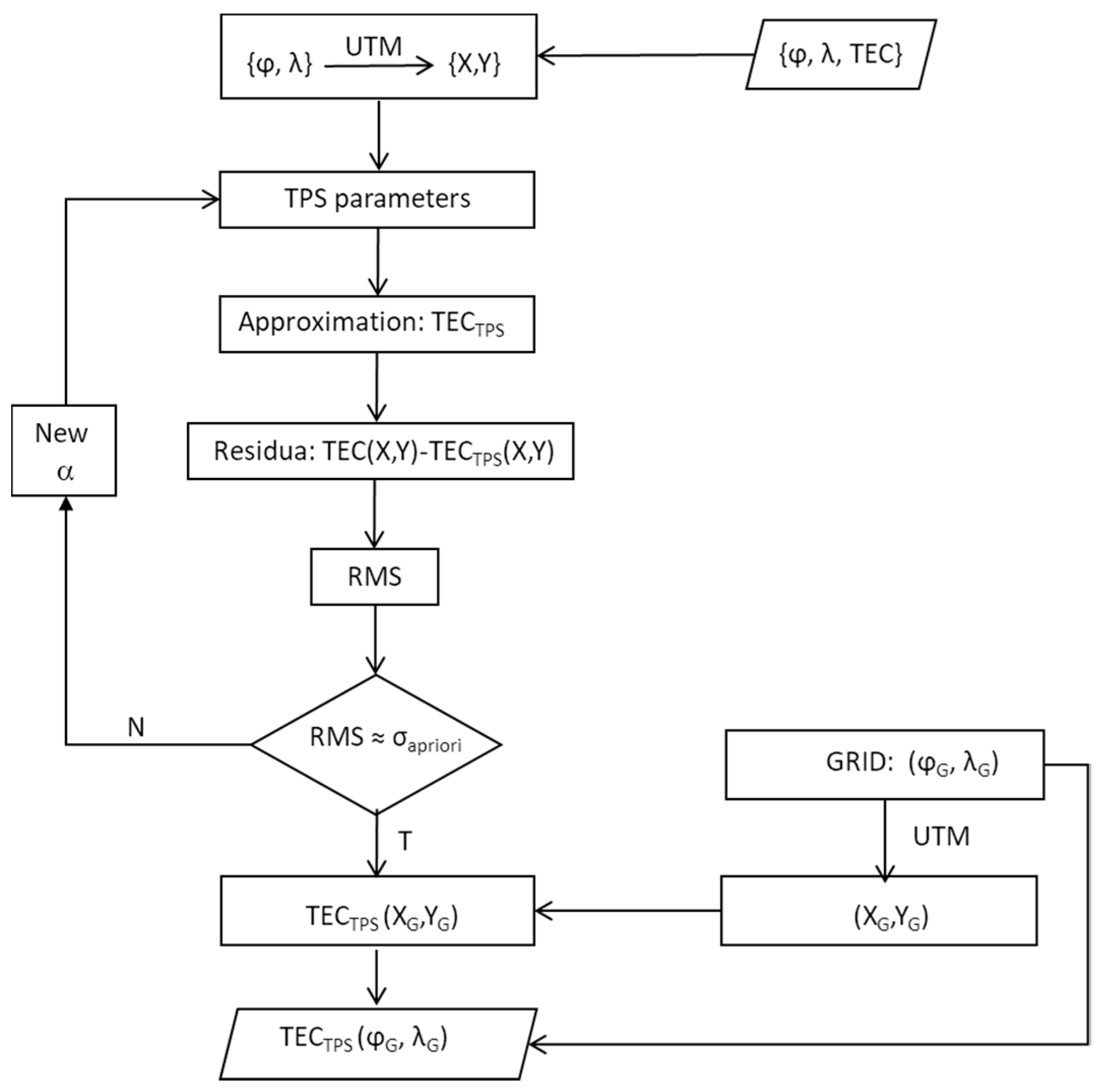
Figure 1 shows a schematic diagram of TPS implementation for the TEC modelling. Since the initial scattered vertical TEC data are given on ellipsoid , they have to be mapped onto the plane. We use the Universal Transverse Mercator (UTM) projection for this purpose. After the TPS parameter estimation according to Equation (6) with an initial value of , the smoothed TECTPS values are determined for the data points . Deviations of these TPS-modelled values from the given TEC data allow for root mean error (RMS) calculation. The received value is compared with an a priori accuracy () of TEC data. If these values are significantly different from each other, the parameter is modified and a new TPS function is determined. In another case, the ellipsoidal grid is mapped onto the plane by means of UTM projection and TECTPS values () are calculated. Finally, TECTPS values are merged with the ellipsoidal grid. The approximation parameter depends strongly on the data to be modelled. We use values of the order of 10−10 for TEC data smoothing and interpolation.
3. Numerical Results and Discussion
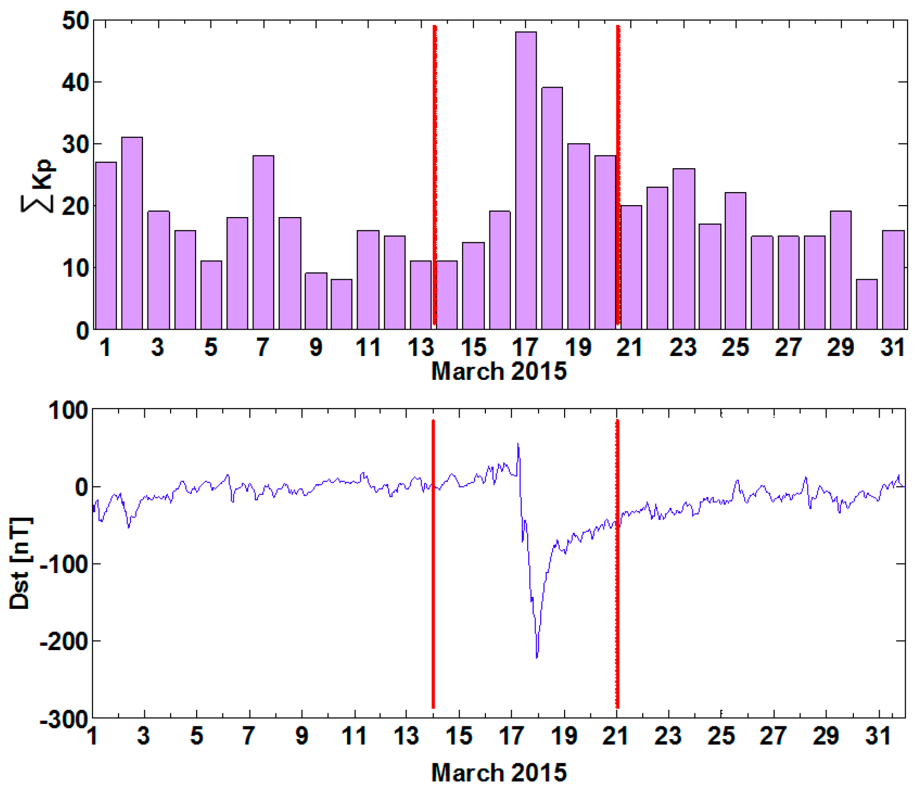
The quality of the presented ionosphere model (UWM-rt1) was tested by a comparison to the five available ionosphere products: IGS, UQRG, JPL, CODG and ESA GIMs. In addition, the reference sTEC variability was compared during the selected 7 days (14–20 March 2015) characterized by varied ionosphere conditions. Figure 2 depicts the disturbance storm time index (Dst) and the variation of daily ΣKp index. As one can see in the figure, the test period includes the ionospheric storm that took place on 17 March 2015 (DoY 76/2015). This is the so-called St. Patrick storm—the strongest disturbance in the ionosphere in 2015. The test period also includes three quiet days before the storm 14–16 March (DoY 73–75/2015), representing the regular state of the ionosphere, and three days after the main phase of the storm, 18–20 March (DoY 77–79/2015), representing the recovery phase. The quiet days were characterized by max ΣKp = 19, while during stormy days ΣKp reached 48 and Dst dropped down to −225 nT. In the recovery phase of the storm, maximum daily ΣKp amounted to 39.
UWM-rt1 is based solely on precise un-differenced dual-frequency carrier phase data from over 200 stations of ground GNSS (GPS + GLONASS) networks. For the data preprocessing, the 30-s sampling interval is used (data cleaning, cycle slip detection, etc.). In order to reduce errors associated with the SLM mapping function, the elevation cut-off angle for GNSS observations was set to 30 degrees. Decreasing the cut-off angle would increase the number of available observations, but low elevation data may introduce errors due to the inaccuracy of the SLM. The final TEC maps are provided with 1 min intervals.
3.1. Self-Consistency Analysis
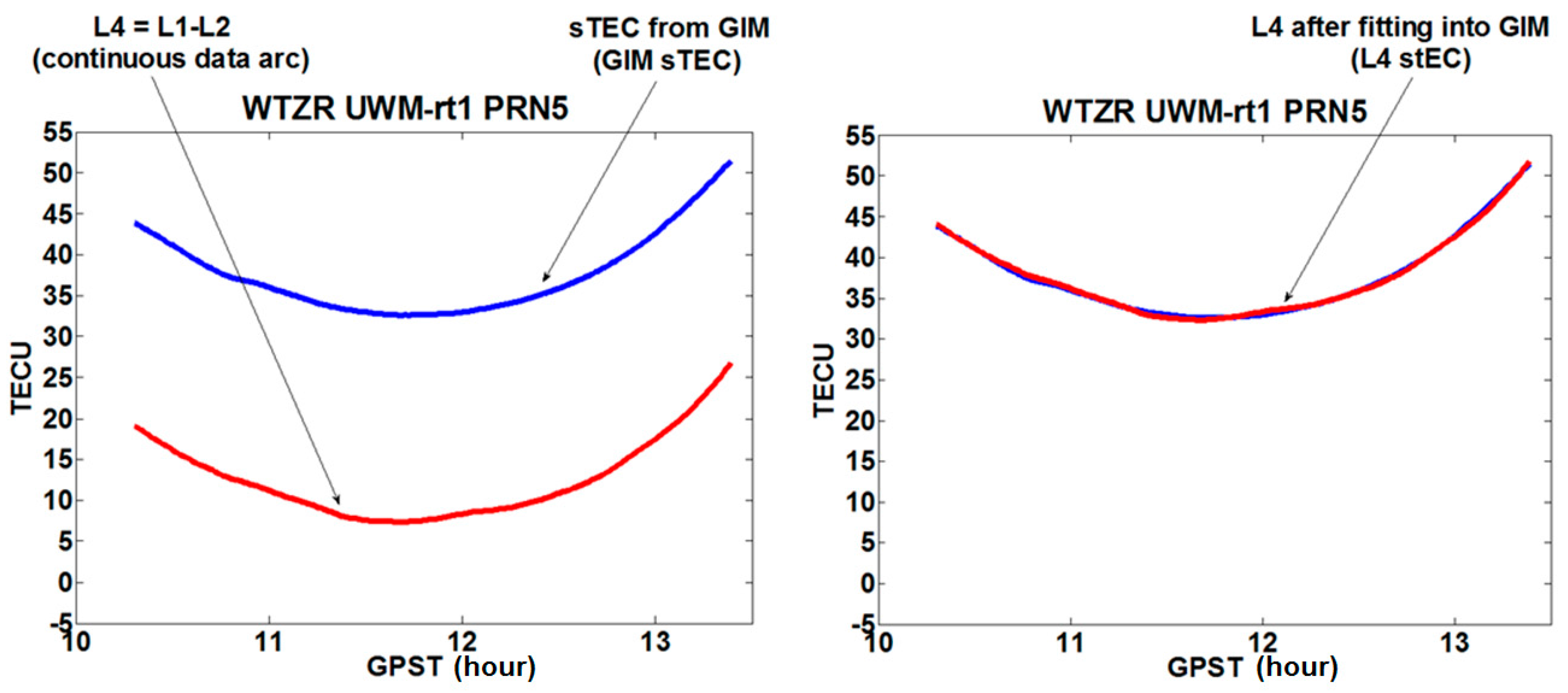
In the presented approach, UWM-rt1 and other tested ionospheric maps were used independently to calibrate sTEC for each continuous carrier phase observational arc. Note that L4 observable data precisely represents changes in the ionospheric delay, and therefore in sTEC. However, this data is biased by the carrier phase bias () that has to be removed by the sTEC calibration procedure. The calibration procedure is as follows:
- Firstly, a geometry-free linear combination (L4) of carrier phase observations is formed for each continuous data arc (red line, Figure 3 left panel);
- next, sTEC for the same satellite arc extracted from a tested model (GIM_sTEC) is calculated (blue line, Figure 3 left panel);
- then, carrier phase bias is estimated by fitting carrier phase data (L4) into GIM_sTEC, resulting in calibrated sTEC (L4_sTEC) (red line, Figure 3 right panel).
In our approach to the self-consistency analysis, post-fit residuals between L4_sTEC and GIM_sTEC were evaluated. Since L4_sTEC is based on real GNSS observations, it precisely reflects actual ionospheric TEC variations and, therefore, may serve as a reference for GIM_sTEC. However, one has to note that the absolute level of L4_sTEC is driven by the TEC level from a particular GIM used for calibration. For statistical analysis of the validated maps, 12 reference stations from EPN networks located in Central and Western Europe were selected (Figure 4). Note that these stations were excluded from UWM-rt1 model calculation.
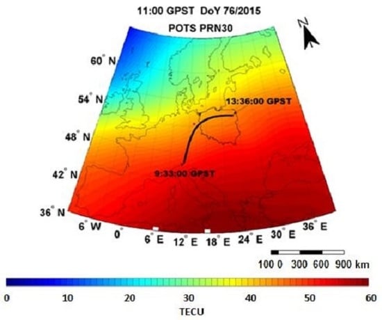
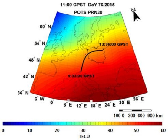
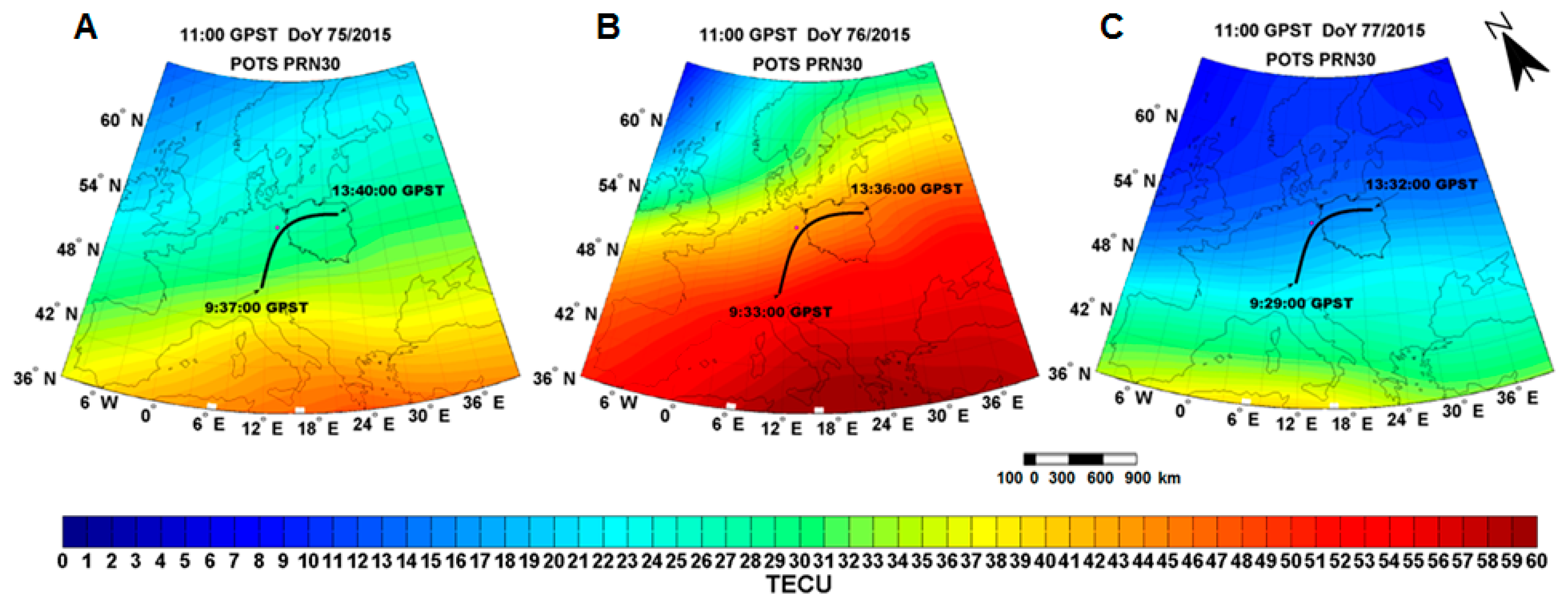
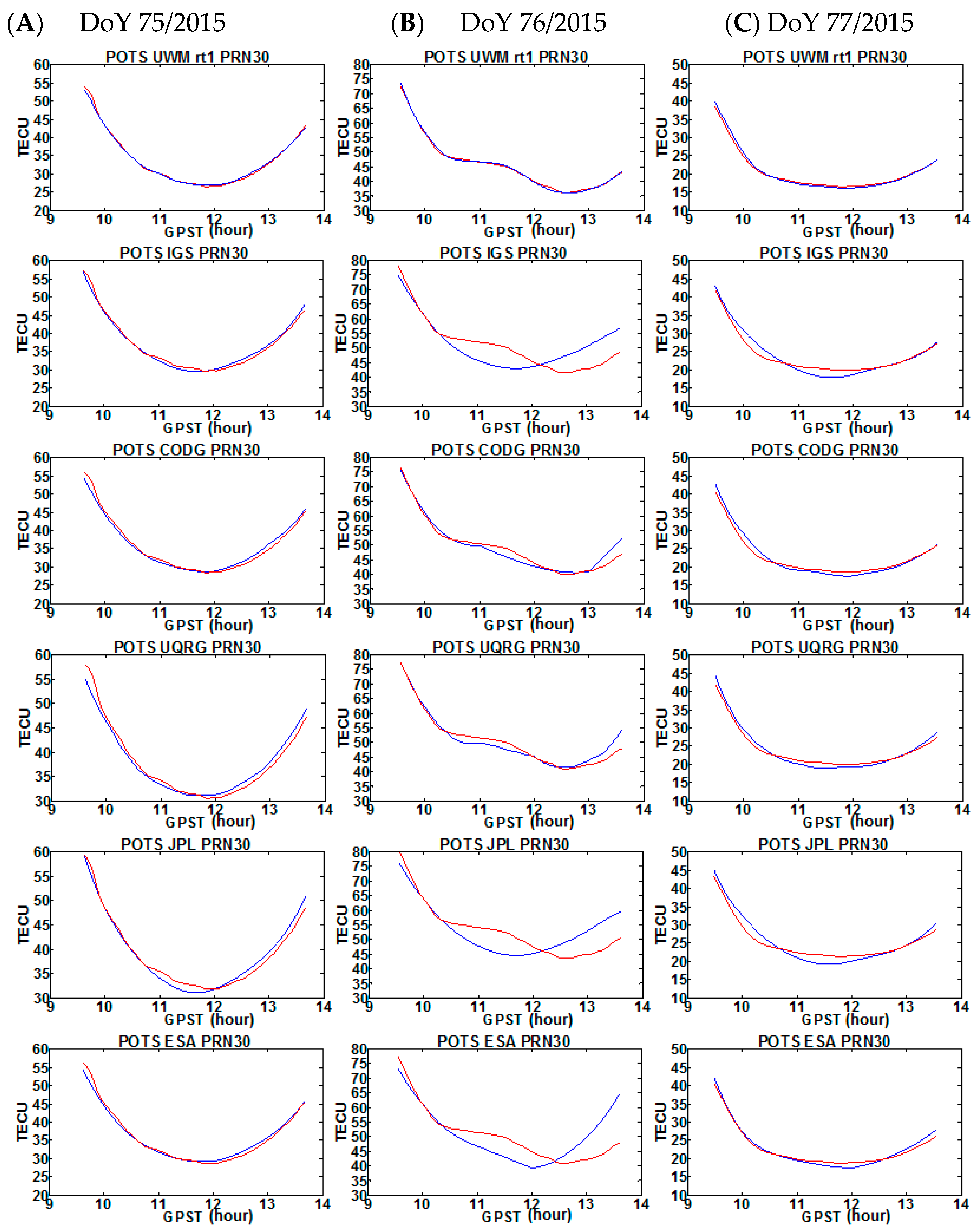
Figure 5 presents example TEC maps derived from the UWM-rt1 model on a quiet day before the storm (DoY 75, A), the stormy day (DoY 76, B) and one day after the storm (DoY 77, C), all at 11.00 GPST (GPS system time). In addition, the ionosphere track of the GPS PRN30 satellite observed by POTS station is presented in the figure. Note that this track covers several hours and it is superimposed on the TEC maps to show its spatial location.
In the analysis, the post fit residuals—between sTEC from the calibrated carrier phase data arcs and the sTEC from the GIMs used for the calibration—were used as a GIMs quality indicator. In the example provided in Figure 6, both L4_sTEC (red) and GIM_sTEC (blue) for PRN30 data arcs are presented. According to this figure, on a geomagnetically quiet day, the sTEC values calculated from all of the six tested maps show quite good agreement with the reference L4_sTEC. However, a significant increase in sTEC residuals is observed on the disturbed day. It can be seen that only the UWM-rt1 model is characterized by good correspondence of GIM_sTEC and L4_sTEC during the ionospheric storm. Out of the remaining five ionosphere models, it is evident that CODG maps perform significantly better than IGS, UQRG, JPL and ESA GIMs. On the quiet day, after the storm, the residuals decreased for all models. However, UWM-rt1 and CODG models still show better fitting to the L4 data. Numerical values of the resulting overall RMS are provided in Table 1 and discussed below.
The statistics concerning the RMS of the post fit residuals for the analyzed TEC maps for all days and stations are presented in Table 1 and Figure 7. The results for the stormy day are marked with bold font. The daily RMS for the particular models was similar during three quiet days before the storm. The RMS did not exceed 1 TECU, and in the case of the UWM-rt1 maps amounted to ~0.4 TECU. In this period, the RMS for CODG maps reached up to ~0.6 TECU, ~0.8 TECU for the IGS maps, whilst for the other evaluated maps the RMS exceeded 0.9 TECU.
The stormy day (DoY 76/2015) provided the most challenging conditions for all models. However, the RMS for the UWM-rt1 was still under 1 TECU, reaching up to ~0.6 TECU, while the RMS for the ESA maps even exceed 2 TECU. The RMS values for CODG, UQRG, IGS and JPL maps amounted to ~1.14, ~1.32, ~1.67 and ~1.81 TECU, respectively. The increased RMS was caused by higher spatial and temporal variability of the ionosphere during the geomagnetic storm. This variability is not properly reproduced by the global TEC maps. This is also reflected in the example presented in Figure 6 (B panel). A possible way to better model the state of the disturbed ionosphere may be to increase the GIMs’ resolutions—both spatial and temporal. This, however, may require very dense networks of GNSS receivers that are not available in many areas.
During the recovery stage of the storm (DoY 77/2015), the negative phase was observed with low TEC values, which was also reflected in lower RMS. The RMS of post-fit residuals in the case of the UWM-rt1 maps was very low (~0.2 TECU), whilst other GIMs varied from ~0.5 TECU (UQRG and CODG) to ~0.7–0.8 TECU (remaining maps). The following days were characterized by an increased RMS level that even reached 1.2 TECU for ESA. However, in the case of UWM-rt1 maps, the RMS remained very low (0.2 TECU).
The overall RMSs based on all days and satellite arc data are presented in Table 2. It can be seen that the RMS for the UWM-rt1 maps amounted to 0.3 TECU, and was three times lower than in the case of the global IGS, JPL maps, and almost four times lower than in the case of the ESA maps. The overall RMS for CODG and UQRG maps was the lowest among global maps and amounted to ~0.6 and ~0.8 TECU, respectively.
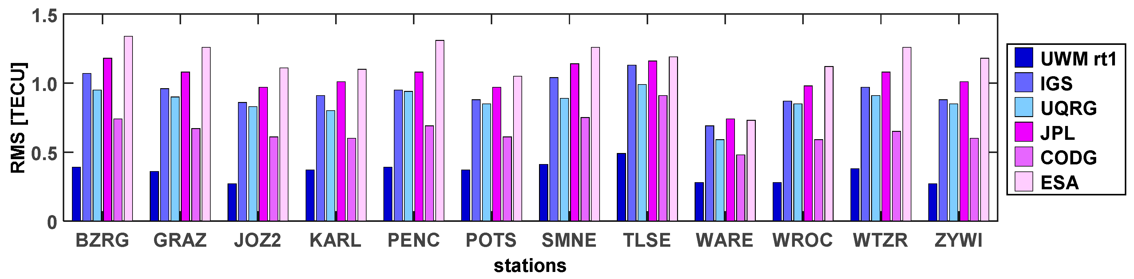
In addition, average RMSs for all analyzed days and satellite arcs were calculated separately for each test station. As one can see in Figure 8, the results are consistent with the results presented in Table 2. For all selected days, the average RMS reached the lowest values for the UWM-rt1 model, while the highest RMSs were observed for the ESA and JPL GIMs. Again, CODG maps present the highest accuracy among global TEC maps. There are no large variations between the results for individual stations. However, the lowest RMS was observed for WARE station.
4. Conclusions
In this contribution, we presented our approach to regional ionospheric TEC modelling based on processing un-differenced GNSS carrier phase data and TPS parametrisation. The resulting TEC maps were analyzed for self-consistency under varying ionosphere conditions, including storm-time geomagnetic disturbances. The results were compared to selected popular GIMs provided by IGS, CODE, ESA, JPL and UPC. It was shown that our regional solution was characterized by 2–3 times lower RMS compared to these maps. It was also observed that during the storm, the RMS for all models increased by a factor of 2, but our approach was the only one with a RMS clearly below 1 TECU. This confirms the applicability of the TPS-based approach in accurate regional ionosphere modelling. Future steps to be taken in the development of our model will include global modelling and validation using altimeter data.
Acknowledgments
The research is supported by grant No. UMO-2013/11/B/ST10/04709 from the Polish National Center of Science.
Author Contributions
Anna Krypiak-Gregorczyk conceived and designed the experiments, processed and analyzed the data, and wrote most of the article. Pawel Wielgosz helped to design the experiments and analyze the results. Andrzej Borkowski wrote the TPS section and carried out TPS processing.
Conflicts of Interest
The authors declare no conflict of interest. The founding sponsors had no role in the design of the study; in the collection, analyses, or interpretation of data; in the writing of the manuscript, and in the decision to publish the results.
References
- Alizadeh, M.M.; Schuh, H.; Schmidt, M. Ray tracing technique for global 3-D modeling of ionospheric electron density using GNSS measurements. Radio Sci. 2015, 50, 539–553. [Google Scholar] [CrossRef]
- Leick, A.; Rapoport, L.; Tatarnikov, D. GPS Satellite Surveying, 4th ed.; J. Wiley and Sons: Hoboken, NJ, USA, 2015; pp. 496–509. [Google Scholar]
- Hu, G.; Abbey, D.A.; Castleden, N.; Featherstone, W.E.; Earls, C.; Ovstedal, O.; Weihing, D. An approach for instantaneous ambiguity resolution for medium- to long-range multiple reference station networks. GPS Solut. 2005, 9, 1–11. [Google Scholar] [CrossRef]
- Wielgosz, P. Quality assessment of GPS rapid static positioning with weighted ionospheric parameters in generalized least squares. GPS Solut. 2011, 15, 89–99. [Google Scholar] [CrossRef]
- Khodabandeh, A.; Teunissen, P.J.G. Array-aided multifrequency GNSS ionospheric sensing: Estimability and precision analysis. IEEE Trans. Geosci. Remote Sens. 2016, 54, 5895–5913. [Google Scholar] [CrossRef]
- Kashani, I.; Wielgosz, P.; Grejner-Brzezinska, D.A. The impact of the ionospheric correction latency on long baseline instantaneous kinematic GPS positioning. Surv. Rev. 2007, 39, 238–251. [Google Scholar] [CrossRef]
- Schunk, R.W.; Scherliess, L.; Sojka, J.J.; Thompson, D. Global Assimilation of Ionospheric Measurements (GAIM). Radio Sci. 2004, 39, RS1S02. [Google Scholar] [CrossRef]
- Bilitza, D.; McKinnell, L.A.; Reinisch, B.; Fuller-Rowell, T. The international reference ionosphere today and in the future. J. Geodesy 2011, 85, 909–920. [Google Scholar] [CrossRef]
- Nava, B.; Radicella, S.M.; Azpilicueta, F. Data ingestion into NeQuick 2. Radio Sci. 2011, 46, RS0D17. [Google Scholar] [CrossRef]
- Gao, Y.; Liao, X.; Liu, Z.Z. Ionosphere modeling using carrier smoothed ionosphere observations from a regional GPS network. Geomatica 2002, 56, 97–106. [Google Scholar]
- Stanislawska, I.; Juchnikowski, G.; Cander, L.R.; Ciraolo, L.; Bradley, P.A.; Zbyszynski, Z.; Swiatek, A. The kriging method of TEC instantaneous mapping. Adv. Space Res. 2002, 29, 945–948. [Google Scholar] [CrossRef]
- Wielgosz, P.; Grejner-Brzezinska, D.A.; Kashani, I. Regional ionosphere mapping with kriging and multiquadric methods. J. Glob. Position. Syst. 2003, 2, 48–55. [Google Scholar] [CrossRef]
- Orùs, R.; Hernández-Pajares, M.; Juan, J.M.; Sanz, J. Improvement of global ionospheric VTEC maps by using kriging interpolation technique. J. Atmos. Sol. Terr. Phys. 2005, 67, 1598–1609. [Google Scholar] [CrossRef]
- Krypiak-Gregorczyk, A.; Wielgosz, P.; Jarmołowski, W. A new TEC interpolation method based on the least squares collocation for high accuracy regional ionospheric maps. Meas. Sci. Technol. 2017, 28, 045801. [Google Scholar] [CrossRef]
- Schaer, S. Mapping and Predicting the Earth’s Ionosphere Using the Global Positioning System. Ph.D. Thesis, Astronomical Institute, University of Berne, Bern, Switzerland, 1999. [Google Scholar]
- Hernández-Pajares, M.; Juan, J.M.; Sanz, J.; Orus, R.; Garcia-Rigo, A.; Feltens, J.; Komjathy, A.; Schaer, S.; Krankowski, A. The IGS VTEC Maps: A Reliable Source of Ionospheric Information since 1998. J. Geodesy 2009, 83, 263–275. [Google Scholar] [CrossRef]
- Schmidt, M.; Dettmering, D.; Moßmer, M.; Wang, Y.; Zhang, J. Comparison of spherical harmonic and B spline models for the vertical total electron content. Radio Sci. 2011, 46, 1–8. [Google Scholar] [CrossRef]
- Rovira-Garcia, A.; Juan, J.M.; Sanz, J.; González-Casado, G. A World-Wide Ionospheric Model for Fast Precise Point Positioning. IEEE Trans. Geosci. Remote Sens. 2015, 53, 4596–4604. [Google Scholar] [CrossRef]
- Zus, F.; Deng, Z.; Heise, S.; Wickert, J. Ionospheric mapping functions based on electron density fields. GPS Solut. 2017, 21, 873–885. [Google Scholar] [CrossRef]
- Hernandez-Pajares, M.; Roma-Dollase, D.; Krankowski, A.; Garcia-Rigo, A.; Orús-Perez, R. Methodology and consistency of slant and vertical assessments for ionospheric electron content models. J. Geodesy 2017, 91, 1–10. [Google Scholar] [CrossRef]
- Hernández-Pajares, M.; Juan, J.M.; Sanz, J.; Aragon-Angel, A.; Garcia-Rigo, A.; Salazar, D.; Escudero, M. The ionosphere: Effects, GPS modeling and the benefits for space geodetic techniques. J. Geodesy 2011, 85, 887–907. [Google Scholar] [CrossRef]
- Feltens, J. The International GPS Service (IGS) ionosphere working group. Adv. Space Res. 2003, 31, 205–214. [Google Scholar] [CrossRef]
- Feltens, J. Development of a new three-dimensional mathematical ionosphere model at European space agency/European space operations centre. Space Weather. 2007, 5, 1–17. [Google Scholar] [CrossRef]
- Mannucci, A.; Wilson, B.; Yuan, D.; Ho, C.; Lindqwister, U.; Runge, T. Global mapping technique for gps-derived ionospheric total electron content measurements. Radio Sci. 1998, 33, 565–582. [Google Scholar] [CrossRef]
- Hernández-Pajares, M.; Juan, J.; Sanz, J. New approaches in global ionospheric determination using ground gps data. J. Atmos. Sol. Terr. Phys. 1999, 61, 1237–1247. [Google Scholar] [CrossRef]
- Brunini, C.; Meza, A.; Azpilicueta, F.; Zele, M.A.V. A new ionosphere monitoring technology based on GPS. Astrophys. Space Sci. 2004, 290, 415–429. [Google Scholar] [CrossRef]
- Bosy, J.; Graszka, W.; Leonczyk, M. ASG-EUPOS—A multifunctional precise satellite positioning system in Poland. Eur. J. Navig. 2007, 5, 2–6. [Google Scholar]
- Krypiak-Gregorczyk, A.; Wielgosz, P.; Krukowska, M. A new ionosphere monitoring service over the ASG-EUPOS network stations. In Proceedings of the 9th International Conference Environmental Engineering (9th ICEE), Vilnius, Lithuania, 22–23 May 2014. [Google Scholar]
- Krypiak-Gregorczyk, A.; Wielgosz, P. Carrier phase bias estimation of geometry-free linear combination of GNSS signals. GPS Solut. 2017. under review. [Google Scholar]
- Lin, L. Remote sensing of ionosphere using GPS measurements. In Proceedings of the 22nd Asian Conference on Remote Sensing, Singapore, 5–9 November 2001. [Google Scholar]
- Shagimuratov, I.; Baran, L.W.; Wielgosz, P.; Yakimova, G.A. The structure of mid- and high-latitude ionosphere during September 1999 storm event obtained from GPS observations. Ann. Geophys. 2002, 20, 665–671. [Google Scholar] [CrossRef]
- Wielgosz, P.; Krypiak-Gregorczyk, A.; Borkowski, A. Regional Ionosphere Modeling Based on Multi-GNSS Data and TPS Interpolation. In Proceedings of the Baltic Geodetic Congress (BGC Geomatics), Gdansk, Poland, 22–25 June 2017; pp. 287–291. [Google Scholar]
- Duchon, J. Interpolation des fonctions de deux varianles suivant le principle de la flexion des plaques minces. R.A.I.R.O. Anal. Numer. 1976, 10, 5–12. [Google Scholar]
- Borkowski, A.; Keller, W. Global and local methods for tracking the intersection curve between two surfaces. J. Geodesy 2005, 79, 1–10. [Google Scholar] [CrossRef]
Figure 1.
Schematic diagram of vertical total electron content (vTEC) modelling by thin plate splines (TPS).
Figure 1.
Schematic diagram of vertical total electron content (vTEC) modelling by thin plate splines (TPS).

Figure 2.
Variations of ΣKp and Dst indices during March 2015. The vertical red lines highlight the seven test days (14–20 March 2015).
Figure 2.
Variations of ΣKp and Dst indices during March 2015. The vertical red lines highlight the seven test days (14–20 March 2015).

Figure 3.
Scheme of the L4 data fitting into Global Ionosphere Maps’ (GIM) slant TEC (sTEC) (sTEC calibration).
Figure 3.
Scheme of the L4 data fitting into Global Ionosphere Maps’ (GIM) slant TEC (sTEC) (sTEC calibration).

Figure 4.
Locations of EUREF Permanent network (EPN) station used in the statistical analysis.
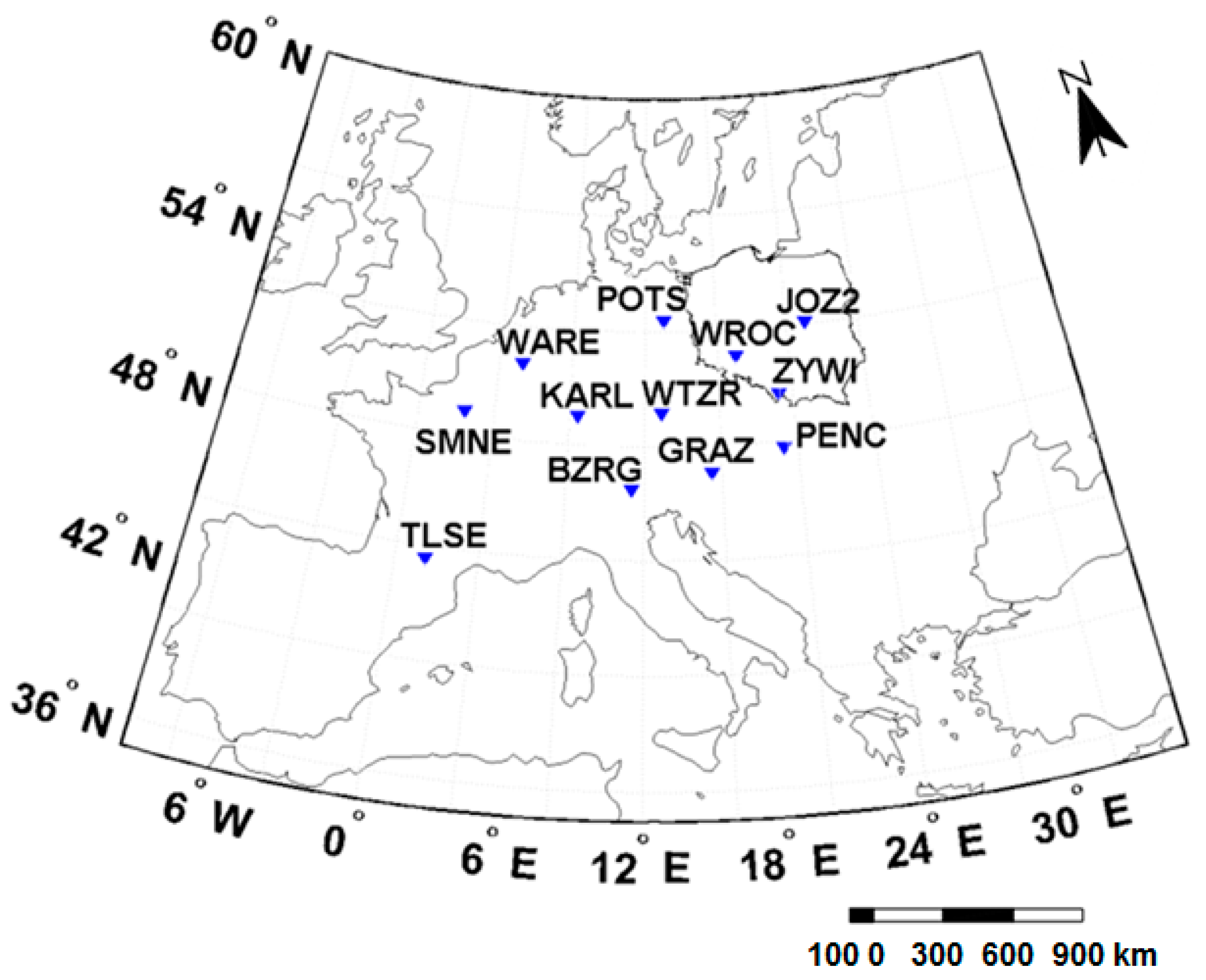
Figure 5.
Example TEC maps derived from the UWM-rt1 model on a quiet day before the storm (A), the stormy day (B) and one day after the storm (C) all at 11:00 GPST. Dark lines represent tracks of the GPS PRN30 satellite observed by POTS station.
Figure 5.
Example TEC maps derived from the UWM-rt1 model on a quiet day before the storm (A), the stormy day (B) and one day after the storm (C) all at 11:00 GPST. Dark lines represent tracks of the GPS PRN30 satellite observed by POTS station.

Figure 6.
sTEC for selected PRN arcs from calibrated geometry-free L4 (L4_sTEC—red) and selected GIMs (GIM_sTEC—blue) on the quiet day before the storm (A), the stormy day (B) and one day after the storm (C).
Figure 6.
sTEC for selected PRN arcs from calibrated geometry-free L4 (L4_sTEC—red) and selected GIMs (GIM_sTEC—blue) on the quiet day before the storm (A), the stormy day (B) and one day after the storm (C).

Figure 7.
Daily RMS distribution for all analyzed TEC maps (TECU).
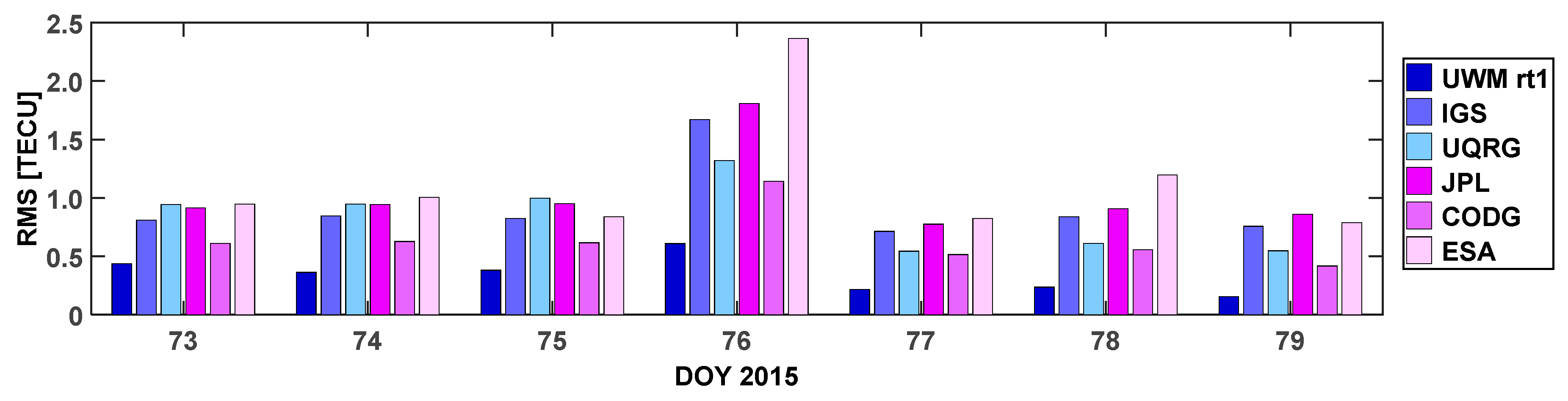
Figure 8.
Average RMS based on all days and satellite arcs for selected test stations.


Table 1.
Root mean error (RMS) of post fit residuals for the analyzed TEC maps (TECU). The stormy day is marked with bold font. UWM-rt1—our regional maps, IGS—International GNSS Service global maps, UQRG—high-rate maps provided by Technical University of Catalonia, JPL—global maps from Jet Propulsion Laboratory, CODG—global maps from Center for Orbit determination in Europe, ESA—global maps from European Space Agency.
| DOY | UWM-rt1 | IGS | UQRG | JPL | CODG | ESA |
|---|---|---|---|---|---|---|
| 73 | 0.44 | 0.81 | 0.94 | 0.91 | 0.61 | 0.95 |
| 74 | 0.36 | 0.85 | 0.95 | 0.94 | 0.63 | 1.00 |
| 75 | 0.38 | 0.83 | 1.00 | 0.95 | 0.62 | 0.84 |
| 76 | 0.61 | 1.67 | 1.32 | 1.81 | 1.14 | 2.36 |
| 77 | 0.22 | 0.71 | 0.54 | 0.78 | 0.52 | 0.82 |
| 78 | 0.24 | 0.84 | 0.61 | 0.91 | 0.56 | 1.20 |
| 79 | 0.15 | 0.76 | 0.55 | 0.86 | 0.42 | 0.79 |
Table 2.
The overall RMS based on all analyzed days, stations and satellite arcs (TECU).
| UWM-rt1 | IGS | UQRG | JPL | CODG | ESA |
|---|---|---|---|---|---|
| 0.34 | 0.92 | 0.84 | 1.02 | 0.64 | 1.14 |
© 2017 by the authors. Licensee MDPI, Basel, Switzerland. This article is an open access article distributed under the terms and conditions of the Creative Commons Attribution (CC BY) license (http://creativecommons.org/licenses/by/4.0/).
Share and Cite
MDPI and ACS Style
Krypiak-Gregorczyk, A.; Wielgosz, P.; Borkowski, A. Ionosphere Model for European Region Based on Multi-GNSS Data and TPS Interpolation. Remote Sens. 2017, 9, 1221. https://doi.org/10.3390/rs9121221
AMA Style
Krypiak-Gregorczyk A, Wielgosz P, Borkowski A. Ionosphere Model for European Region Based on Multi-GNSS Data and TPS Interpolation. Remote Sensing. 2017; 9(12):1221. https://doi.org/10.3390/rs9121221
Chicago/Turabian StyleKrypiak-Gregorczyk, Anna, Pawel Wielgosz, and Andrzej Borkowski. 2017. "Ionosphere Model for European Region Based on Multi-GNSS Data and TPS Interpolation" Remote Sensing 9, no. 12: 1221. https://doi.org/10.3390/rs9121221
Note that from the first issue of 2016, this journal uses article numbers instead of page numbers. See further details here.