A New Method for Acquisition of High-Resolution Seabed Topography by Matching Seabed Classification Images


1
School of Geodesy and Geomatics, Wuhan University, Wuhan 430079, China
2
Institute of Marine Science and Technology, Wuhan University, Wuhan 430079, China
3
School of Power and Mechanical Engineering, Wuhan University, Wuhan 430072, China
4
School of Resources and Environmental Engineering, Anhui University, Hefei 230601, China
*
Author to whom correspondence should be addressed.
Remote Sens. 2017, 9(12), 1214; https://doi.org/10.3390/rs9121214
Submission received: 13 October 2017
/
Revised: 11 November 2017
/
Accepted: 22 November 2017
/
Published: 24 November 2017
(This article belongs to the Section Ocean Remote Sensing)
Abstract
:The multibeam echo sounders (MBES) can acquire accurate positional but low-resolution seabed terrain and images, whereas side scan sonars (SSS) can only acquire inaccurate positional but high-resolution seabed images. In this study, a new method for superimposing corrected-positional SSS images on multibeam bathymetric terrain is proposed to obtain high-resolution and accurate-positional seabed topography using traditional MBES and SSS. Three steps, including the normalization by the z-score, sediment classification by the k-means++ algorithm, and denoising processing using morphological operations, are processed for both MBES and SSS images to obtain the corresponding sediment images. Next, a segmented matching method is given based on the common sediment distributions and features of MBES and SSS sediment images. The two kinds of sediment images are matched segmentally using the speeded up robust features algorithm and random sample consensus algorithm. Then, the positions of SSS images are corrected segmentally using thin plate splines based on matching points. Finally, the corrected SSS image is superimposed on MBES bathymetric terrain, based on positional relationship. The proposed method was verified through experiments, and high image resolution and high position accuracy seabed topography were obtained. Moreover, the performances of the method are discussed, and some conclusions are drawn according to the experiments and discussions.

1. Introduction
Multibeam echo sounders (MBES) and side scan sonars (SSS) have wide applications in remote sensing of seabed topography or morphology [1,2,3,4,5]. The SSS, which usually has higher frequency than MBES, has certain advantages, such as low cost and easy installation, and its ability to obtain large-scale, high-resolution, and high-signal-to-noise ratio (SNR) seabed images [1]. Given that the towing operation mode is often adopted in SSS measurement, the positions of an SSS towfish are estimated through the headings and positions of the surveying vessel and towing length and depth. SSS images often suffer low accuracy position because of varying vessel operation and hydrological conditions, and have a limited preciseness in applications. An MBES is usually installed at the bottom of a surveying vessel to obtain accurate positional bathymetry and backscatter image, but the resolution and SNR of MBES surveying results are much lower than those of SSS image, and further decrease with the increase in water depth. Many actual applications have verified the difficulty of obtaining highly accurate high-resolution terrain and image through traditional MBES or SSS in the measurement of a middle or deep water directly [6].
At present, the above problem can be solved in three main ways. The first is application of light detection and ranging (LiDAR), which can measure the topography and physical characteristics of the seafloor by, respectively, pulsing sound or laser light. However, its application depth is limit less than 50 m [7]. The second is the introduction of new instruments, which combine MBES and phase-differencing bathymetric technique [8]. These new instruments are called multi-phase echo sounder (MPES), such as Kongsberg’s GeoSwath and Edgetech 6205 bathymetric SSS. MPESs can acquire accurate positional bathymetric data and high-resolution seabed image simultaneously, but they have disadvantages, such as expensiveness, low penetration, and limitations in terms of water depth (<200 m). The complementarity of SSS and MBES data implies another method to obtain high-resolution and accurate positional seabed topography through the superimposition of two-dimensional (2D) SSS images on three-dimensional (3D) MBES terrain. Researchers have attempted to study the superposition method in various ways. Yang et al. [6] used the similarity of MBES topographic contours and SSS image contours to carry out the matching and superposition. Zhao et al. [9] focused on matching the MBES terrain images and SSS images. These methods were based mainly on the correlation of MBES terrain and SSS images, but often suffer weak correlation and incorrect matching because of poor relation between terrain and seabed images. Moreover, matching 3D MBES terrain and 2D SSS images directly is difficult because of different data types. The terrain data present seabed undulating, whereas sonar images reflect seabed features and seabed sediment variations, and are affected by the beam patterns, scattering models, and image processing algorithms. Hence, these methods may be ineffective when dealing with undulating seabed with single sediment or flat seabed with various sediments.
Fortunately, modern MBESs can record time-sequence backscatter strength (BS) data (i.e., snippet) and resolutions of snippet images are higher than those of the images formed by traditional average beam BS. Both MBES and SSS images are formed using BSs, and thus can reflect similar seabed textures, targets on the seabed, and distributions and variations of seabed sediments. Therefore, solving the correlation problem in the current matching methods becomes possible. Hughes Clarke [10] stated the equivalence of MBES and SSS images. Le [11] analyzed the influencing factors on the qualities of MBES and SSS images, and found them to be very similar. Various 2-D sonar image registration techniques that are based on feature-based [12], template-based [13], region-based [14], as well as Fourier-based approaches [15] have been explored. The speeded up robust features (SURF) algorithm based on point feature matching shows good performance when applying to sonar data if we can control signal-to-noise ratio of the sonar data or transform sonar image to other form [16]. Therefore, this study proposes a new method for the superimposition of SSS images and MBES terrain based on the matching of the two types of sonar images. Through superimposition, inaccurate positional problem, which limits the applications of SSS image, can be solved, and high-resolution and accurate positional seabed topography is obtained with the results of traditional MBES and SSS.
The structure of this paper is as follows. Section 2 introduces the characteristics of MBES and SSS images. Section 3 provides the detailed method of superimposition of SSS image and MBES terrain, including the acquisitions of MBES and SSS sediment images, segmental matching between MBES and SSS sediment images, determination of transformation relations between MBES and SSS images, and the superimposition of corrected SSS image and MBES terrain. Section 4 presents the validation and analysis of the proposed method through experiments. Section 5 provides the corresponding discussion. Section 6 presents several beneficial conclusions drawn from the experiments and discussions.
2. MBES and SSS Images
Given that the equal-angle-spacing mode (Figure 1a) is often adopted by MBES, the distances across the ping sounding points would be enlarged with the increase in beam incident angle and water depth. The SNR of MBES BS is usually low because of the interferences of the main lobes, side lobes, and scattering echoes [11]. The frequency of MBES is usually lower than SSS for better penetrability. A higher-frequency SSS is applied mainly to obtain higher-resolution acoustic images and to find underwater targets; hence, it does not have sounding ability. SSSs are often towed behind a vessel to avoid hull noise and interferences from side and wake flows, as shown in Figure 1b. The SSS beam pattern is simpler than MBES. These features of SSS cause significantly higher resolution and SNR of the SSS image than those of MBES. The MBES transducer is installed generally at the vessel bottom; thus, its position can be obtained accurately by combining GPS positioning solution, vessel heading and attitude, coordinates of GPS, and MBES transducer in vessel frame system. The position of SSS towfish is often estimated by combining vessel position and heading and horizontal towing distance. The estimations of horizontal towing distance and towfish heading are often inaccurate because of vessel operation, wind, and wave, thereby resulting in inaccurate positional images.
The above causes lead to accurate positional MBES terrain and low-resolution MBES images, and high-resolution but inaccurate-positional SSS images, especially in the measurement of middle and deep water. This complementarity of MBES and SSS measurement results implies that obtaining high-resolution, high-SNR, and accurate positional seabed topography is possible by combining high-resolution SSS images with accurate positional MBES terrain. The connection between MBES and SSS measurement results is that MBES and SSS images can both reflect seabed objects and sediment variations [10,11,17,18,19]. The effects of the beam pattern (Figure 1), angular response (AR) (Figure 2a), and residual error of time varying gain (TVG) causes radiometric distortion in MBES data and decreases the quality of MBES image [20]. Similarly, the quality of SSS image is also decreased because of radiometric distortions that are caused by TVG residual, sonar altitude, beam pattern, and angular response [21]. Therefore, MBES and SSS data preprocessing is necessary to eliminate these effects and highlight seabed features and sediment variations before the superposition of SSS image and MBES terrain.
3. Superposition of SSS Images and MBES Terrain
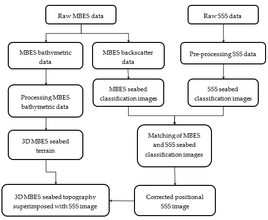
Usually, the BSs of MBES and SSS are recorded in dB and displayed by sonar image in gray levels, respectively; hence, the proposed methods use sediment images rather than backscatter intensity images. As described above, MBES and SSS images have a strong correlation in reflecting seabed sediment variations and features [11,17,18,19,22]. Therefore, sonar images will be used as the link of the two sets of measurement results in the superposition of SSS image and MBES terrain. Based on the link, the superposition can be performed by obtaining seabed sediment images of MBES and SSS, matching of the MBES and SSS sediment images, correcting the position of the SSS image, and superimposing the corrected positional SSS image on MBES terrain. The complete process is depicted in detail, as follows.
3.1. Acquisitions of Sediment Images
The sediment images of MBES and SSS are obtained in three steps, including the normalization of BS data of MBES and SSS, k-mean++ unsupervised classification of the two types of sonar images, and denoising of the two sediment images. For example, for the MBES image, the following explains the acquisition of sediment image.
(1) Angular data normalization using the z-score
MBES images are affected mainly by beam patterns, angular responses, and TVG residuals [22]. The standard score or the z-score is used for the normalization of along-track BSs to remove these angle-related effects and make BS variations of the same sediment in a consistent range [23]. For a BS sequence of the same incident angle with mean μ and standard deviation σ, the z-score of a BS is as follows:
Figure 3a,b show the BS sequences and the corresponding z-score sequences at the incidence angle of 2° and 30°, respectively. BS data in different intensity ranges (Figure 3a) are unified into the same range (Figure 3b) after normalization. The variation trend of BSs of different sediments is still reflected in the normalized z-score sequences. After normalization, classifying BSs of different incident angles to different seabed sediments becomes possible.
(2) Sediment classification by k-means++ algorithm
Distributions of seabed sediments are usually unknown in uncharted waters, and unsupervised classification is generally used to obtain seabed classifications without a priori sediment knowledge. The k-means++ algorithm is simple and applicable for data mining [24]; hence, it was selected in this study. For a segment of raw MBES waterfall image (Figure 4a), the sediment classification image (Figure 4c) can be obtained using the k-means++ algorithm with the classification number k of 2 from the corresponding normalized z-score image (Figure 4b).
(3) Denoising of sediment image by morphology operations
In Figure 4c, noises in sediment images are serious because of MBES data noises. The morphology opening and closing operations are used in combination for the denoising of the sediment image in this study. Dilation and erosion are two fundamental operations in morphological image processing. The dilation operation usually uses a structuring element for probing and expanding the shapes contained in the input image, while the erosion operation is the opposite operation [25]. For a sediment image A, the opening is the dilation of the erosion of A by an image element B, and the closing is the erosion of the dilation of A by B.
where ○ and ● are opening and closing operations and and denote the dilation and erosion operations, respectively.
The opening operation is used mainly to connect objects incorrectly segmented into smaller slices, whereas the closing operation is used mainly to remove small spots introduced by image noise [25]. Using closing then opening operations, noises in Figure 5c were removed effectively, and the distributions of these two sediments become clear.
The above process for obtaining MBES sediment image is also appropriate for forming SSS sediment image. The difference in processing is that SSS images are affected by angle-related effects (similar to those in the MBES image) and angle-unrelated effect (i.e., TVG residuals in the along-track direction) [26,27]. This angle-unrelated effect can be removed according to the variation of the towfish altitude [21,26]. After removal, the process similar as the above is adopted to obtain the SSS sediment image, as shown in Figure 6.
3.2. Segmental Matching Based on Sediment Distributions and Features
Time-varying factors, such as towing horizontal lengths, towfish headings, and depths, influence the accurate estimation of towfish positions, as well as the geo-coding SSS images, whereas MBES images have accurate positions. Therefore, the positions of the SSS sediment image can be corrected by the transformation relation achieved from segmental matching of the common sediment distributions and features of SSS and MBES sediment images. Five steps are included in the segmental matching algorithm and detailed as follows.
- (1)
- Geocode the MBES sediment image of a survey line according to instantaneous locations of MBES transducer.
- (2)
- Geocode the SSS sediment image in the same water region as the MBES sediment image according to the instantaneous estimation locations of SSS towfish.
- (3)
- Select a segment of SSS sediment image with m × n along the survey line, and determine the co-located and slightly larger than m × n MBES image segment from the MBES sediment image when considering the positional error. The segment principle is discussed in Section 5.4.
- (4)
- Extract the common feature point pairs and match the two image segments by the SURF algorithm [28]. A detailed process includes the following steps:
- (a)
- Detect the feature points from the MBES image segment and the corresponding SSS one using SURF.
- (b)
- Describe each feature point with a multidimensional vector.
- (c)
- Match the feature points according to the nearest vector distance of different feature points.
- (d)
- Use random sample consensus (RANSAC) algorithm to check the consistencies of the angles and distances of the matching vector pairs to eliminate mismatching.
- (5)
- Repeat steps 3–4 until the matchings in all segments are carried out.
The SURF is used for searching feature point pairs in the above matching. SURF is a robust image recognition and description algorithm, which is generally considered as the improved scale-invariant feature transform (SIFT) algorithm [29]. The SURF is several times faster and more robust than SIFT in image transformations [28,30,31]. Zhao et al. achieved SSS image matching of adjacent surveying lines by SURF and verified feasibility of SURF in sonar image matching [22]. Therefore, the SURF is adopted for segmental matching in this study. The SURF consists mainly of interest point detection, local neighborhood description, and matching. The SURF uses square-shaped filters as an approximation of Gaussian smoothing and a blob detector based on the Hessian matrix to find interest points to accelerate the process. The Haar wavelet is also applied to assign the point orientation and describe the region around the point. These feature point pairs are matched by SURF after the extraction and description of feature points. During matching, the description vectors of matching feature points should have the shortest Euclidean distance.
The RANSAC algorithm is used for removing the abnormal matching point pair in the above matching. RANSAC is an iterative algorithm to estimate the parameters of a mathematical model from a set of observed data containing outliers. Applying the RANSAC is necessary to check matched feature point pairs to avoid mismatching. Because both of the MBES and SSS images are geo-coded, the feature points in MBES and SSS images have absolute coordinates. We could use the relative positional deviation as the geo-distance parameter to control the matching results. The geo-distance parameter is set by referring to the estimated positioning accuracy of the SSS towfish. The positioning accuracy of the SSS towfish can be estimated by combining the accuracies of the vessel location, the horizontal length of the towing cable, and the towfish heading. In this paper, the geo-distance parameter is set as 5 m. The checking process using RANSAC is depicted as follows:
- (1)
- Select a random subset of the matching point pairs and named it as the hypothetical inliers.
- (2)
- Calculate the relative geo-distance distribution model, namely the mean and twice the standard deviation of the relative positional deviation from the set of hypothetical inliers. If the absolute value of the relative geo-distance distribution model is more than the given geo-distance parameter as mentioned the above, the hypothetical inliers will be given up and go back to step 1; otherwise, continue to step 3.
- (3)
- All other matching point pairs are tested against the relative geo-distance distribution model. The points that fit the estimated model well are considered as part of the consensus set.
- (4)
- The model is reasonable if sufficient matching pairs have been classified as part of the consensus set. In addition, the model may be improved by re-estimating it using all members of the set.
3.3. Position Correction of SSS Images Using Thin-Plate Splines
After matching, the positional relationship of the matching point pairs in the two corresponding image segments can be calculated, and the SSS image segment can be corrected to the same position as the corresponding MBES image segment through the transformation relation. The thin plate spline (TPS) is the 2D analog of the cubic spline in 1D [32,33]. Given a set of data points f, a weighted combination of thin plate splines centered on each data point gives the interpolation function I that passes through the points exactly, while minimizing the so-called bending energy. Bending energy is defined as the integral over of the squares of the second derivatives:
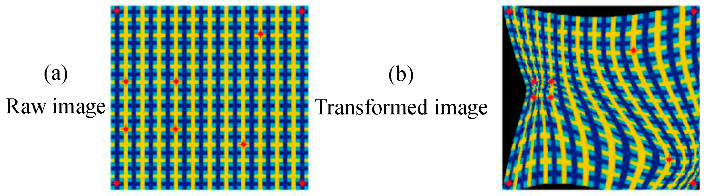
The TPS as the non-rigid transformation model is used widely in image warping corrections [31,33,34], as shown in Figure 7. Thus, it is adopted in this study.
The processing steps, including matching, calculation of transformation relation, and positional correction of SSS image, are used for each MBES and co-located SSS image segment to correct entire SSS images.
3.4. Superimposition of SSS Images and MBES Terrain
After the positional correction, the location of SSS image is improved efficiently. The resampling is done to the corrected SSS images by considering the seabed texture features and sediment variation to obtain perfect SSS images. The superimposition of MBES terrain on SSS images is performed depending on the location relationship. Figure 8 presents this superimposition.
4. Experiment and Analysis
4.1. Data Acquisition
Measurements of MBES and SSS were performed in the water area with 0.6 km × 1.8 km and 300–320 m of water depth, in the South China Sea. Sediments were investigated by seabed sampling and contain mainly silt and sand. In the MBES measurement, KONGSBERG EM 3002 with 300 kHz of the operating frequency, max 130° of the angular sector, and 131 beams was adopted. In the SSS measurement, EdgeTech 4100P SSS with 400 kHz operating frequency, 112 m recorded max slang range, 20° sonar depression angle, and 0.5° and 50° of the plane and vertical beam were towed 200 m underwater. Five MBES survey lines and four SSS survey lines were carried out in the water area. The MBES data with approximately 100 m swath width, 0.5 m ping interval, and 800 echoes in a ping and the SSS data with approximately 150 m scanning width, 0.27 m ping interval, and 7502 samples in a ping were obtained. After data preprocessing, the MBES sounding terrain, geocoded MBES snippet, and SSS images are displayed in Figure 9b–d. The detailed terrain cannot be displayed clearly in the margin of MBES swath because of equal-angle spacing mode, and the SSS image is clearer than the MBES snippet image because the image resolution of the former is higher than the latter. The measurement results show the necessity of superimposing the high-resolution SSS image on the high-accuracy MBES terrain.
4.2. Superimposition of SSS Image and MBES Terrain
Segmental matching is the core of the proposed method. In the proposed segment method, MBES and SSS BS data in the same sub-region were extracted for this experiment. Before using them, two sets of data were pre-processed to remove the radiometric distortion effects on the sonar image initially. Through three steps, including angular data normalization, seabed sediment classification, and denoising, sediment images were carried out using z-score, k-mean++ algorithm, and morphology operations. The MBES and SSS sediment images were obtained and geocoded. The processing to obtain the sediment images is depicted in Figure 10a–f for the SSS image and in Figure 10A–F for the MBES image. The MBES (Figure 10F) and SSS images (Figure 10f) were divided into three segments. MBES and SSS images in the corresponding segments were matched following the segmental matching method depicted in Section 3.2. The size of each segment depends on the distributions of sediments and features, as depicted in Section 5.4. The common feature point pairs of MBES and corresponding SSS segmental images are extracted by SURF. The transformation relationship between three segmental images is calculated and used for position correction of the SSS segmental image using TPS. The matchings are depicted in Figure 10R1–R3.
In Figure 10a,b, the BSs of ping inner echoes were much larger than those of outer ones. While this phenomenon disappeared in Figure 10c after data normalization, the BSs of the same sediment at different incident angles were nearly consistent, and sediment types and distributions became clear relative to Figure 10b. Two sediment types were classified from Figure 10c and shown in Figure 10d, using the k-mean++ algorithm. Some noises appear in Figure 10d because of noises in the raw SSS BS data. Therefore, the morphology operations were used for improving Figure 10d. Figure 10e shows the improved image. The distributions of the two sediments and seabed features in Figure 10e were clear. Figure 10A–E shows similar processes to obtain MBES sediment images. The above results show that the proposed steps were efficient in the acquisitions of SSS and MBES sediment images. Figure 10f,F show the geocoded SSS and MBES sediment images, respectively.
In Figure 10f,F, distributions of sediment and seabed features in the two images are similar, showing that matching of MBES and SSS images based on common sediment distributions and seabed features is reasonable. The sediment distributions and features in the SSS sediment image are slightly distorted and malposed relative to those in the MBES sediment image because of inaccurate positions and attitudes of SSS towfish. The feature point pairs of the two sediment images were extracted and matched in the corresponding segments (as shown in Figure 10R1–R3), respectively, using the segmental matching method depicted in this study. The mismatching feature point pairs were removed using the RANSAC algorithm. The transformation relationship in each segment can be calculated using the TPS for position correction of SSS images in the corresponding segment based on the segmental matching results.
Segmental matching can be carried out in the entire water area by adopting the similar processing as the above, as shown in Figure 11. The positional corrections are performed for the SSS images of all the SSS lines using transformation relations obtained in different matching segments. Given adopting the TPS function and segmentally local correction, resampling is done to the corrected SSS images by considering the seabed texture features and sediment variation. Image fusion operation is also performed in the overlapping areas of adjacent survey lines using the wavelet transform method [9]. Because of the time-varying positional error of SSS images, the distributions of sediments and feature shapes in the raw SSS image (Figure 11b) are slightly different from those in the MBES snippet image (Figure 11a). Whereas, a comparison between the corrected SSS image (Figure 11c) and the MBES image (Figure 11a) shows that the distributions of sediments and feature shapes are consistent in the two images and the segmental matching is efficient.
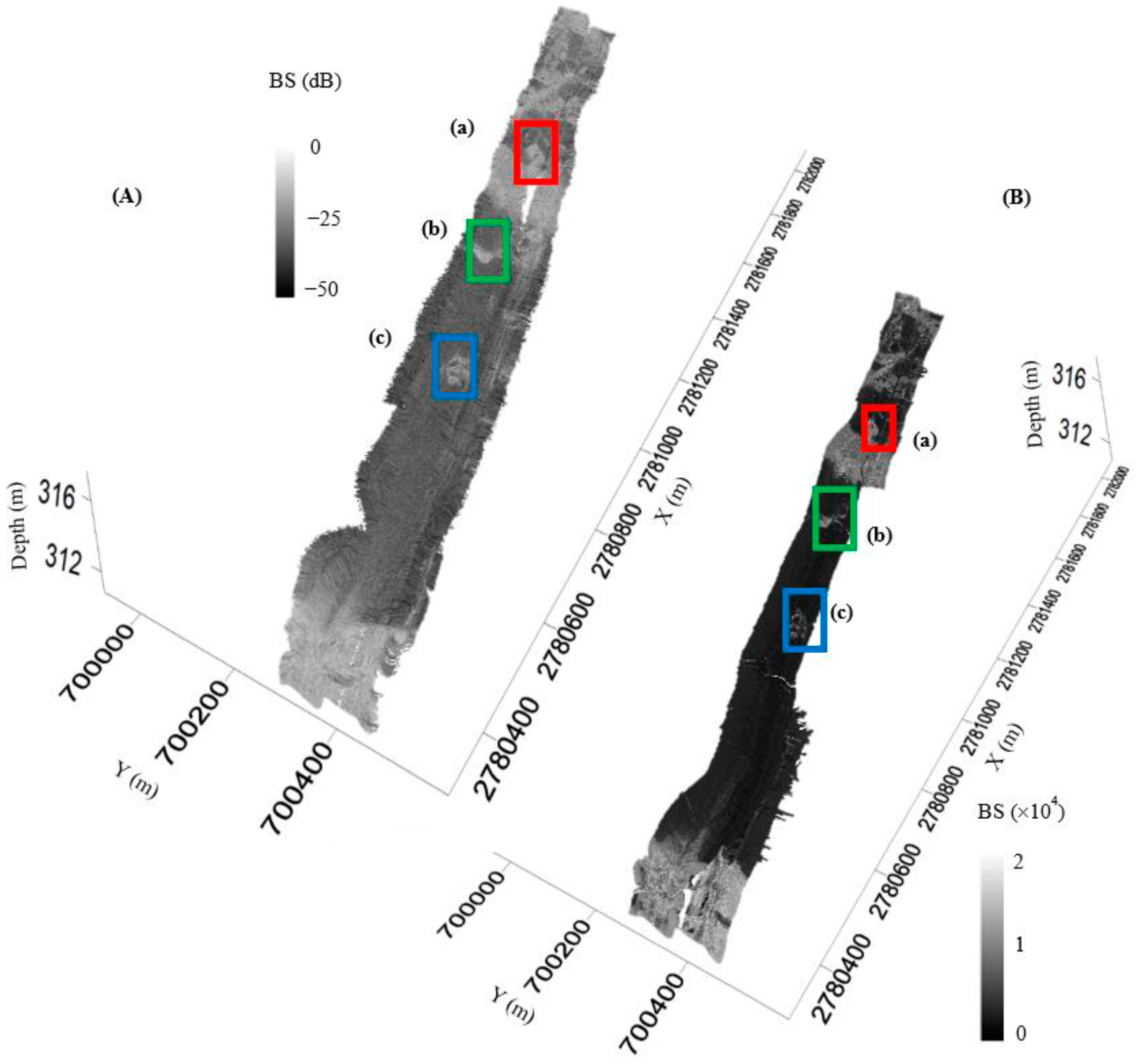
Given that the position accuracy of the corrected SSS image is the same as that of the MBES image and terrain, the superimpositions of the corrected SSS image on the MBES terrain and the MBES snippet image on the MBES terrain can be carried out depending on consistent locations. Figure 12 shows the two superimpositions. The superimpositions of the corrected SSS image and the MBES terrain are more detailed than that of the MBES snippet image and MBES terrain because of the difference of image resolution. Three small areas with seabed targets, marked as (a)–(d) are chosen and enlarged to explain the detailed degree of the superimposition of the corrected positional SSS image and the MBES terrain, as shown in Figure 13. The following can be found in Figure 13.
- (1)
- (2)
- Good consistence between the SSS images and MBES terrains is achieved at the three targets at different positions of the measurement area, and verifying that the segmental matching in consideration of time-varying positional accuracy of SSS towfish is appropriate.
4.3. Matching Accuracy
A segment of SSS sediment image with the significant distributions of sediments and features is extracted from Figure 13a and shown in Figure 14a to assess the matching accuracy quantitatively, as achieved by the proposed method. The feature point pairs are extracted by SURF initially; then, the TPS and traditional rigid transformation are used to correct the image, as shown in Figure 14b,c, respectively. The peach-shape distribution in Figure 14b is slightly larger, whereas that in Figure 14c is slightly less than that in the raw SSS image. This phenomenon means that these transformations changed the point positions of the raw SSS image. The position errors of the corrected SSS feature points are calculated by taking the feature points in the MBES image as reference. The statistical results show that the max, mean, and standard deviations of 18.99, 9.11, and 11.87 m are achieved by the raw SSS image, as 8.00, 3.33, and 3.80 m by the rigid transformation, and as 3.00, 2.50, and 0.67 m by TPS. The result also shows the need to adjust the high-resolution SSS image and superiority of TPS relative to the rigid transformation.
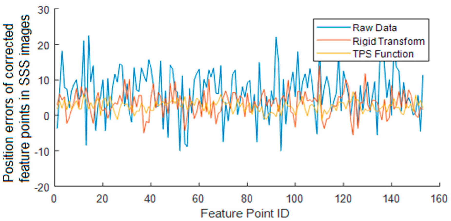
Adopting the process similar to that used in Figure 14, the errors of all feature points in the SSS image in Figure 11b are calculated. Figure 15 and Table 1 show the error distributions and statistical results that are achieved by the two transformations, respectively. Similar conclusion is drawn that the position accuracy achieved by the TPS is better than that by the traditional rigid transformation and much better than that in the raw SSS image. This result proved that the proposed segmented matching and transformation are efficient because of the time-varying position errors are considered.
5. Discussion
5.1. Necessity to Superimpose SSS Image on MBES Terrain
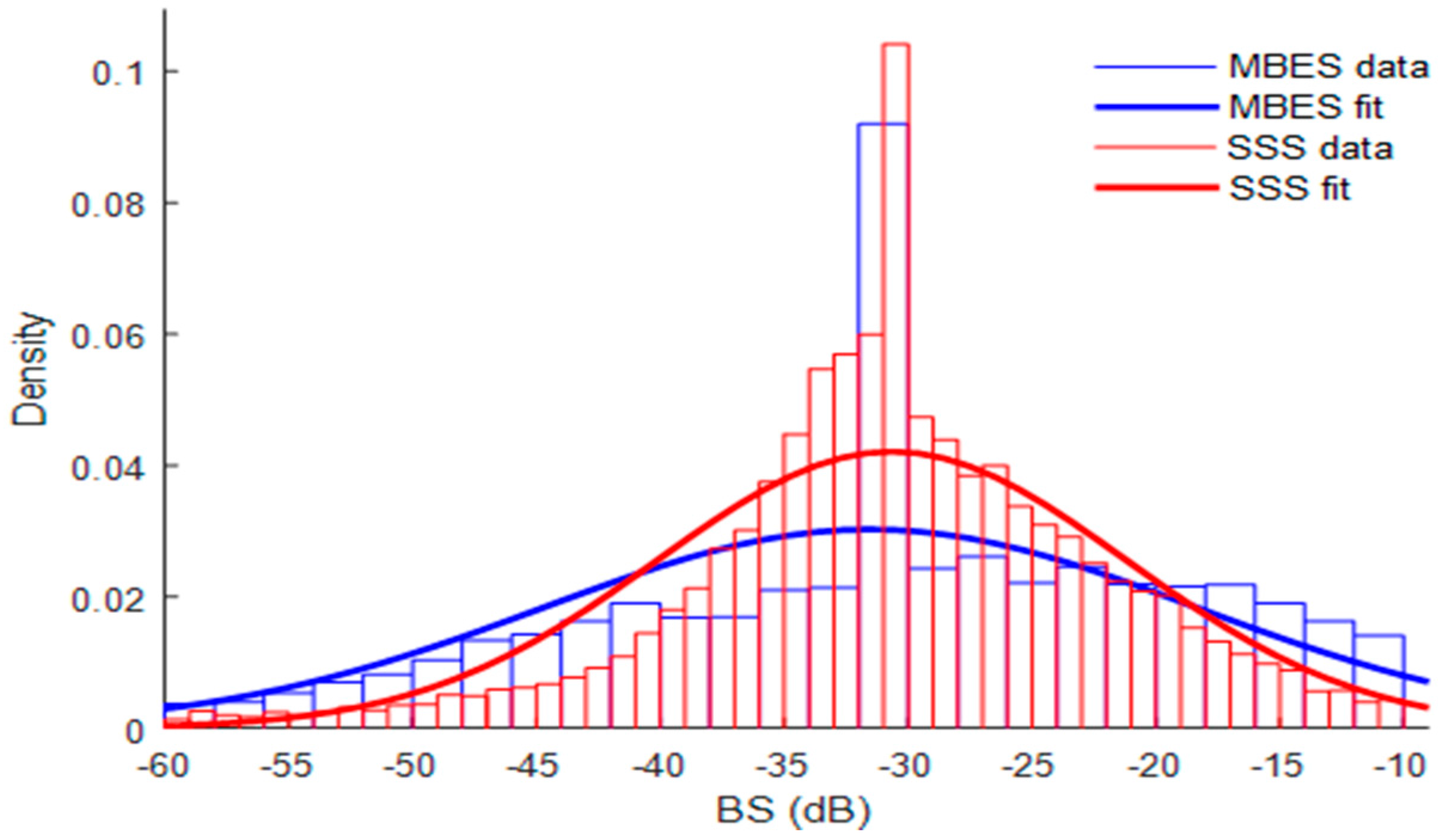
In a randomly selected region, the sample number of MBES and SSS are 92,423 and 4,883,802, respectively. The data resolution of SSS was far larger than that of MBES. The significant difference is caused mainly by the measurement mechanisms of the two sonar systems. SSS image can reflect the more detailed seabed than MBES image. The BSs of the silt sediment in the selected region were analyzed statistically to study the SNR of BS data in reflecting the same sediment, as shown in Figure 16. The distribution of SSS BS data is much denser than that of MBES data. The SSS BS variation range is smaller than that of MBES. The statistical result shows that the SSS image has better SNR than the MBES image. The above result proved the necessity of superimposing SSS image on the MBES terrain to reflect accurately and subtly the sediment variations, texture features, and terrain undulations.
5.2. Possible Features Used in the Matching
The matching of the MBES and SSS sediment images is the basis of this study. The transformation relationship between the two images can only be established through image matching. The superimposition of the SSS images on the MBES terrain can be realized after the position correction of the SSS image. The possible features for matching include seabed undulation, terrain texture, seabed sediment variation, and targets on the seabed. When considering the measurement patterns and equipment performances, the availabilities of these features are analyzed as follows.
- (1)
- Seabed terrain: Both MBES and SSS images are 2D images. Topographic variations may not be reflected in the 2D images. Thus, seabed terrain cannot be used as a feature in the matching.
- (2)
- Seabed sediment variation: Although MBES and SSS images have significant differences in the initial emission energy level, acoustic frequency, and bean pattern, both MBES and SSS images can reflect the variations and distributions of common seabed sediments. These studies proved that seabed sediments can be classified using MBES and SSS BS data [20,35]. Therefore, the sediment variations in MBES and SSS images can be used as common features in the matching of the two types of images.
- (3)
- Seabed targets: Based on the imaging mechanisms of SSS and MBES, large seabed targets should appear in both of the sonar images in theory. However, considering that SSS images have higher resolution and SNR than MBES images, some small seabed targets can be displayed in SSS images, but not in MBES images. According to the principle of sediment classification, the same targets that appear in the two sonar images can also be displayed in their sediment images and used as common features in the matching.
- (4)
5.3. Influencing Factors on the Matching
Targets and sediment variations can be used as the common features in the matching and affect the matching. The matching method also influences the matching.
(1) Distribution density of seabed targets
Ideally, if sufficient targets distribute evenly on the seabed, sufficient matching point pairs can be found for the accurate calculation of the transformation relationship between MBES and SSS sediment images. However, the seabed targets often distribute randomly on the seabed, and the amount may be small, even zero. Matching accuracy can be guaranteed by the matching of both seabed targets and sediment features on the rich-feature seabed. For the poor-feature seabed, the matching can also be performed by enlarging the matching scope. Extending the scope may decrease calculation accuracy of the transformation relation, but it does not have a significant effect on displaying the seabed features in the corrected SSS image [22].
(2) Complexity of seabed sediment variation
In addition to seabed targets, sediment variations are important common features for matching. In a water area, the seabed may consist of several kinds of sediments. The complexity of sediment variation could provide various feature points for the matching, whereas fewer feature points can be extracted and the matching accuracy will become lower for very simple sediment distribution. In homogeneous seabed, fewer or even no feature points can be found, leading to an incorrect transformation relationship. The matching accuracy does not have a significant effect on the SSS image in reflecting the variations of seabed sediment because of homogeneous seabed [22].
(3) Effects of the matching method
The matching method is also an important factor that affects final matching. This study takes the following measurements to decrease the effect.
Segmental matching and position calibration: The position accuracy of the towfish varies with vessel operation and sea conditions because the SSS uses the towing operation mode [22,26]. The segmental matching is proposed in this study to achieve accurate calibration for the SSS image. In the area without feature points, transformation relationships are obtained by interpolating smoothly nearby transformation relationships.
Optimal selection of feature point pairs: Given that the transformation parameters are calculated based on the coordinates of the feature points in segmental images, incorrect feature points affect the calculation directly. During the extraction of feature points, some incorrect ones may be found by SURF. To avoid the mistake, RANSAC algorithm is adopted in the proposed method to guarantee the reliability of the selected feature point pairs.
Distortion of SSS image: Given the low positioning accuracy and residual errors that are caused by imperfect processing, positional distortion exists in SSS images and affects the finding feature point and selecting feature point pairs by the tradition matching methods. SURF has the scale-invariant feature because of adopting Haar-like features and integral image [28]. The good performance of SURF in the matching has been verified by the above experiments.
5.4. Size of Matching Segment
The positional accuracy of SSS images varies with time-varying horizontal distances and headings of the towfish [22,26]. The segmental matching and positional correction of SSS images becomes necessary to improve the position accuracy of SSS images. The segment division follows the following principles:
- (1)
- At least five feature point pairs should be included in the segmental images to guarantee calculation accuracy of transformation.
- (2)
- Setting small size matching segment is necessary to weaken the effect of time-varying errors.
Based on the two principles, the size of the matching segment should change with the distribution and number of extracted feature points. For the rich-feature seabed, the matching segment should be divided into smaller sizes that contain at least five feature points. Whereas for the poor-feature seabed, the matching segment should be expanded to a larger size until the segmental image contains five feature points.
5.5. Applications
In shallow waters, the new-generation MPES can obtain both seabed bathymetric terrain and backscatter images. However, its measurement depth is limited at 200 m. Meanwhile, sampling rates of MBES snippet data are high enough in shallow waters; hence, the advantages of high-resolution SSS images are not very obvious [21]. In middle and deep waters, a SSS towfish can still approach the seabed to obtain high-resolution seabed image, whereas the image resolution of MBES installed on a survey vessel is decreased considerably as the water depth increase because of the equiangular operation model, especially for outer beams [2]. Moreover, MBES images cannot reflect the details of seabed topography and meet the requirements of precise engineering applications. MBES or MPES can also be installed on the autonomous underwater vehicle (AUV) or remotely operated vehicle (ROV) to approach the seabed and acquire both seabed terrain and corresponding backscatter images, such as the measurement in the shallow water [36]. However, the speed of AUV or ROV limits its applications. The proposed method can realize fast acquisition of high-resolution and accurate positional seabed topography, without changing the current operation mode or decreasing the accuracy of the final results. Therefore, the method provides a new way to obtain high-resolution and accurate-positional seabed topography rapidly in middle and deep waters using traditional MBES and SSS. Moreover, the proposed method is also suitable for MBES and SSS data in shallow water, and has advantages like no need for new equipment and relative low cost.
6. Conclusions
The proposed method, the superimposition of SSS images and MBES terrain based on matching of seabed features, considers the angular-related effect, time-varying positioning error in SSS image, and the common underwater targets and seabed sediment distributions in both SSS and MBES images. Therefore, in the proposed method, SSS and MBES images are improved through radiometric and angular response corrections, and the positional accuracy of SSS image is improved using segmental matching common targets and sediment distributions. Thus, the high image resolution and high position accuracy seabed topography can be obtained. The proposed method provides a better way to show fine seabed topography using the survey results of traditional MBES and SSS. These conclusions were verified by the experiments, and the accurate and high-resolution seabed topography is achieved in the experiment.
Acknowledgments
The study is supported by the National Natural Science Foundation of China (coded by 41576107, 41376109, and 41176068), National Science and Technology Major Project (coded by 2016YFB0501703), and the Key Laboratory of Surveying and Mapping Technology on Island and Reef, National Administration of Surveying, Mapping and Geoinfomation (coded by 2015B08). The data in this study are provided by Guangzhou Marine Geological Survey Bureau. The authors are greatly thankful for their support.
Author Contributions
Jianhu Zhao and Junxia Meng conceived and designed the experiments; Junxia Meng designed the proposed method and performed the experiments; Junxia Meng, Jianhu Zhao and Jun Yan analyzed the data; Hongmei Zhang contributed analysis tools; and Jianhu Zhao, Junxia Meng, Hongmei Zhang and Jun Yan wrote the paper.
Conflicts of Interest
The authors declare no conflict of interest.
References
- Blondel, P. Automatic mine detection by textural analysis of cots sidescan sonar imagery. Int. J. Remote Sens. 2000, 21, 3115–3128. [Google Scholar] [CrossRef]
- Hughes Clarke, J.; Mayer, L.; Wells, D. Shallow-water imaging multibeam sonars: A new tool for investigating seafloor processes in the coastal zone and on the continental shelf. Mar. Geophys. Res. 1996, 18, 607–629. [Google Scholar] [CrossRef]
- Fakiris, E.; Papatheodorou, G.; Geraga, M.; Ferentinos, G. An automatic target detection algorithm for swath sonar backscatter imagery, using image texture and independent component analysis. Remote Sens. 2016, 8, 373. [Google Scholar] [CrossRef]
- Degraer, S.; Moerkerke, G.; Rabaut, M.; Van Hoey, G.; Du Four, I.; Vincx, M.; Henriet, J.-P.; Van Lancker, V. Very-high resolution side-scan sonar mapping of biogenic reefs of the tube-worm lanice conchilega. Remote Sens. Environ. 2008, 112, 3323–3328. [Google Scholar] [CrossRef]
- Collier, J.S.; Humber, S.R. Time-lapse side-scan sonar imaging of bleached coral reefs: A case study from the seychelles. Remote Sens. Environ. 2007, 108, 339–356. [Google Scholar] [CrossRef]
- Fanlin, Y.; Ziyin, W.; Zhixing, D.; Xianglong, J. Co-registering and fusion of digital information of multi-beam sonar and side-scan sonar. Geomat. Inf. Sci. Wuhan Univ. 2006, 31, 740–743. [Google Scholar]
- Costa, B.M.; Battista, T.A.; Pittman, S.J. Comparative evaluation of airborne lidar and ship-based multibeam sonar bathymetry and intensity for mapping coral reef ecosystems. Remote Sens. Environ. 2009, 113, 1082–1100. [Google Scholar] [CrossRef]
- Brisson, L.; Hiller, T. Multiphase echosounder to improve shallow-water surveys. Sea Technol. 2015, 56, 10–14. [Google Scholar]
- Zhao, J.; Wang, A.; Guo, J. Study on fusion method of the block image of MBS and SSS. Geomat. Inf. Sci. Wuhan Univ. 2013, 287–290. [Google Scholar] [CrossRef]
- Hughes Clarke, J.E. Applications of multibeam water column imaging for hydrographic survey. Hydrogr. J. 2006, 120, 3. [Google Scholar]
- Le Bas, T.; Huvenne, V. Acquisition and processing of backscatter data for habitat mapping—Comparison of multibeam and sidescan systems. Appl. Acoust. 2009, 70, 1248–1257. [Google Scholar] [CrossRef]
- Johannsson, H.; Kaess, M.; Englot, B.; Hover, F.; Leonard, J. Imaging sonar-aided navigation for autonomous underwater harbor surveillance. In Proceedings of the 2010 IEEE/RSJ International Conference on Intelligent Robots and Systems, Taipei, Taiwan, 18–22 October 2010; pp. 4396–4403. [Google Scholar]
- Thorpe, C. Sonar image processing: An application of template matching through relaxation. In Proceedings of the the 1981 2nd International Symposium on Unmanned Untethered Submersible Technology, Boston, MA, USA, 9 October 1981; pp. 35–52. [Google Scholar]
- Yong, E.W. Investigation of Mosaicing Techniques for Forward Looking Sonar. Master’s Thesis, Heriot-Watt University, Edinburgh, Scotland, UK, 2011. [Google Scholar]
- Hurtós, N.; Ribas, D.; Cufí, X.; Petillot, Y.; Salvi, J. Fourier-based registration for robust forward-looking sonar mosaicing in low-visibility underwater environments. J. Field Robot. 2015, 32, 123–151. [Google Scholar] [CrossRef]
- Aykin, M.D.; Negahdaripour, S. On feature matching and image registration for two-dimensional forward-scan sonar imaging. J. Field Robot. 2013, 30, 602–623. [Google Scholar] [CrossRef]
- SiljestrÖM, P.; Moreno, A.; Rey, J. Technical note seafloor characterization through side scan sonar image processing. Int. J. Remote Sens. 1995, 16, 625–632. [Google Scholar] [CrossRef]
- Bates, C.R.; Oakley, D.J. Bathymetric sidescan investigation of sedimentary features in the tay estuary, scotland. Int. J. Remote Sens. 2004, 25, 5089–5104. [Google Scholar] [CrossRef]
- Hasan, R.; Ierodiaconou, D.; Monk, J. Evaluation of four supervised learning methods for benthic habitat mapping using backscatter from multi-beam sonar. Remote Sens. 2012, 4, 3427–3443. [Google Scholar] [CrossRef]
- Zhao, J.; Yan, J.; Zhang, H.; Meng, J. Two self-adaptive methods of improving multibeam backscatter image quality by removing angular response effect. J. Mar. Sci. Technol. 2017, 22, 288–300. [Google Scholar] [CrossRef]
- Zhao, J.; Yan, J.; Zhang, H.; Meng, J. A new radiometric correction method for side-scan sonar images in consideration of seabed sediment variation. Remote Sens. 2017, 9, 575. [Google Scholar] [CrossRef]
- Zhao, J.; Wang, A.; Zhang, H.; Wang, X. Mosaic method of side-scan sonar strip images using corresponding features. IET Image Process. 2013, 7, 616–623. [Google Scholar] [CrossRef]
- Fonseca, L.; Calder, B. Clustering acoustic backscatter in the angular response space. In Proceedings of the US Hydrographic Conference, Norfolk, VA, USA, 14–18 May 2007. [Google Scholar]
- Arthur, D.; Vassilvitskii, S. K-means++: The advantages of careful seeding. In Proceedings of the Eighteenth Annual ACM-SIAM Symposium on Discrete Algorithms; Society for Industrial and Applied Mathematics: New Orleans, LA, USA, 2007; pp. 1027–1035. [Google Scholar]
- Laganière, R. Opencv 2 Computer Vision Application Programming Cookbook: Over 50 Recipes to Master This Library of Programming Functions for Real-Time Computer Vision; Packt Publishing Ltd.: Birmingham, UK, 2011; p. 277. [Google Scholar]
- Capus, C.; Ruiz, I.T.; Petillot, Y. Compensation for changing beam pattern and residual tvg effects with sonar altitude variation for sidescan mosaicing and classification. In Proceedings of the 7th European Conference on Underwater Acoustics, Delft, The Netherlands, 5–8 July 2004. [Google Scholar]
- Capus, C.G.; Banks, A.C.; Coiras, E.; Ruiz, I.T.; Smith, C.J.; Petillot, Y.R. Data correction for visualisation and classification of sidescan sonar imagery. IET Radar Sonar Navig. 2008, 2, 155–169. [Google Scholar] [CrossRef]
- Bay, H.; Ess, A.; Tuytelaars, T.; Van Gool, L. Speeded-up robust features (surf). Comput. Vis. Image Understand. 2008, 110, 346–359. [Google Scholar] [CrossRef]
- Lowe, D.G. Object recognition from local scale-invariant features. In Proceedings of the Seventh IEEE International Conference on Computer Vision, Kerkyra, Greece, 20–27 September 1999; Volume 1152, pp. 1150–1157. [Google Scholar]
- Luo, J.; Gwun, O. A comparison of sift, pca-sift and surf. Int. J. Image Proc. 2009, 3, 143–152. [Google Scholar]
- Brook, A.; Ben-Dor, E. Automatic registration of airborne and spaceborne images by topology map matching with surf processor algorithm. Remote Sens. 2011, 3, 65–82. [Google Scholar] [CrossRef]
- Bookstein, F.L. Principal warps: Thin-plate splines and the decomposition of deformations. IEEE Trans. Pattern Anal. Mach. Intell. 1989, 11, 567–585. [Google Scholar] [CrossRef]
- Glasbey, C.A.; Mardia, K.V. A review of image-warping methods. J. Appl. Stat. 1998, 25, 155–171. [Google Scholar] [CrossRef]
- Yang, K.; Pan, A.; Yang, Y.; Zhang, S.; Ong, S.; Tang, H. Remote sensing image registration using multiple image features. Remote Sens. 2017, 9, 581. [Google Scholar] [CrossRef]
- Wahba, G. Spline Models for Observational Data; Society for Industrial and Applied Mathematics: Philadelphia, PA, USA, 1990. [Google Scholar]
- Woock, P. Deep-sea seafloor shape reconstruction from side-scan sonar data for auv navigation. In Proceedings of the OCEANS, 2011 IEEE—Spain, Santander, Spain, 6–9 June 2011; pp. 1–7. [Google Scholar]
Figure 1.
Operating modes and beam patterns of multibeam echo sounders (MBES) (a) and side scan sonars (SSS) (b).
Figure 1.
Operating modes and beam patterns of multibeam echo sounders (MBES) (a) and side scan sonars (SSS) (b).

Figure 2.
Incident angle—backscatter strength (BS) curves of MBES (a) and SSS (b) with different types of sea bottom.
Figure 2.
Incident angle—backscatter strength (BS) curves of MBES (a) and SSS (b) with different types of sea bottom.
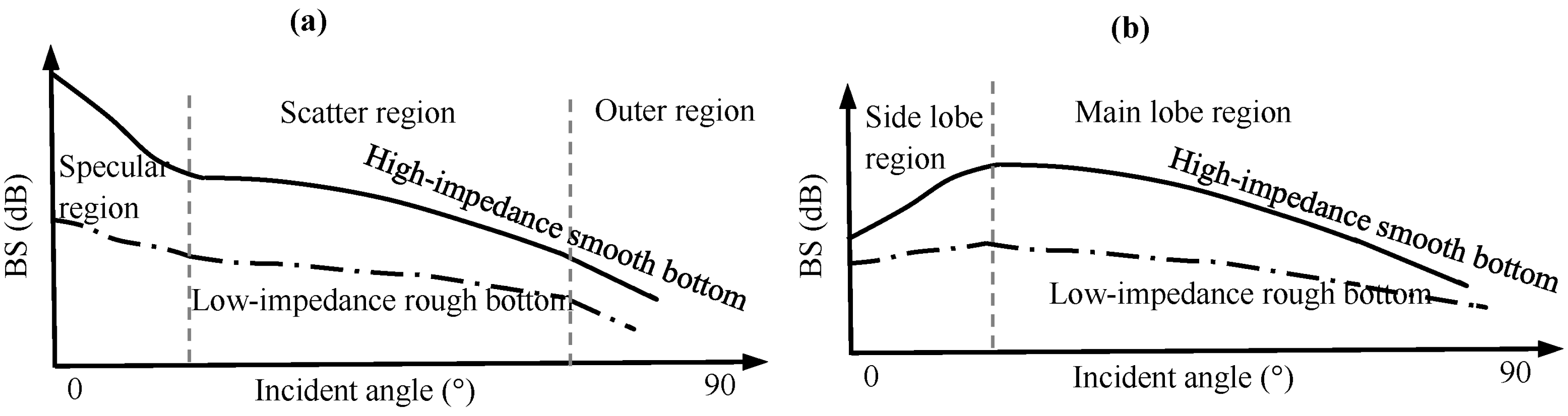
Figure 3.
Normalization of MBES BS data. (a) Along-track BS sequences at incident angles 2° and 30° and (b) corresponding z-score sequences.
Figure 3.
Normalization of MBES BS data. (a) Along-track BS sequences at incident angles 2° and 30° and (b) corresponding z-score sequences.
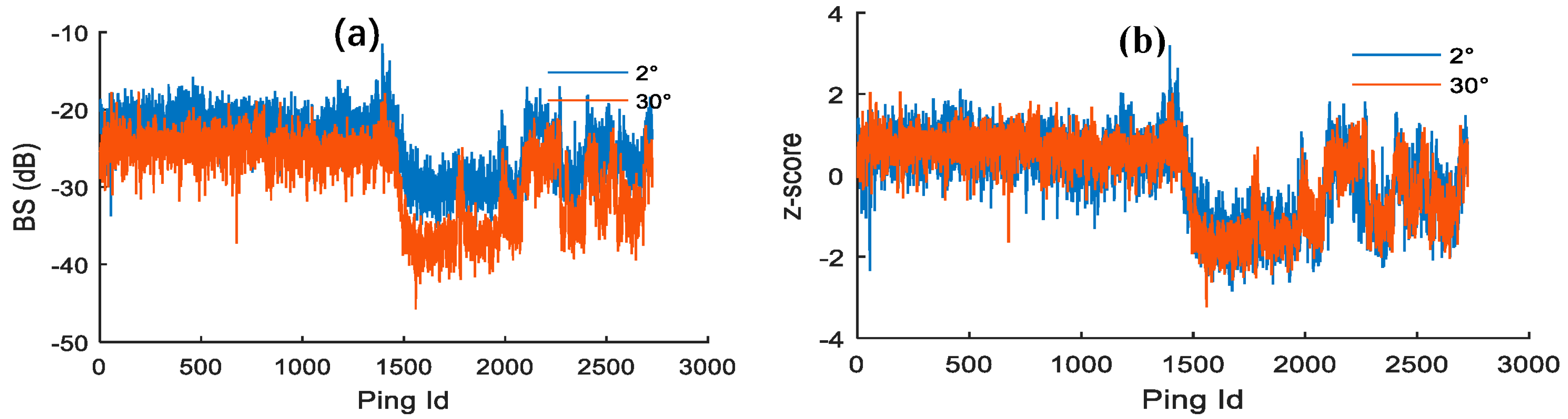
Figure 4.
Seabed classification on MBES waterfall image using the z-score and k-mean++ algorithm. (a) Raw MBES waterfall image; (b) normalized z-score image; and (c) classification result with k = 2. φ is the incident angle of each beam.
Figure 4.
Seabed classification on MBES waterfall image using the z-score and k-mean++ algorithm. (a) Raw MBES waterfall image; (b) normalized z-score image; and (c) classification result with k = 2. φ is the incident angle of each beam.
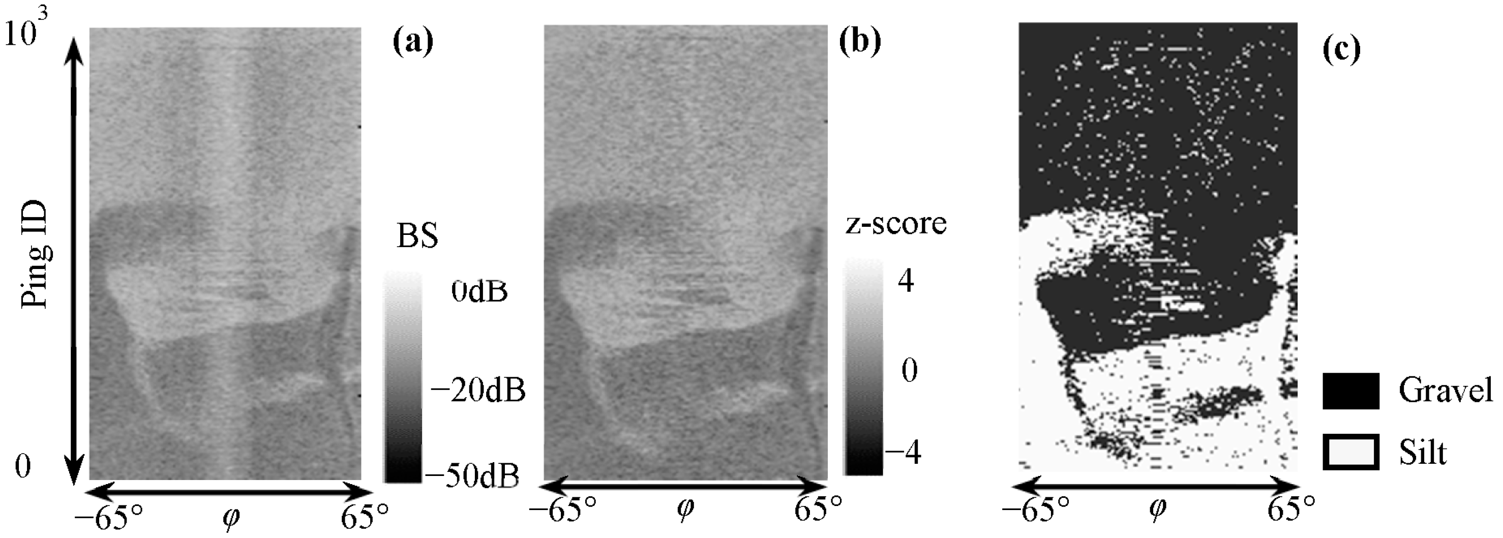
Figure 5.
Denoising of MBES sediment image. (a) Original classification image; (b) image after eliminating noise by closing; and (c) image after connecting the main sediment by opening of (b). φ is the incident angle.
Figure 5.
Denoising of MBES sediment image. (a) Original classification image; (b) image after eliminating noise by closing; and (c) image after connecting the main sediment by opening of (b). φ is the incident angle.
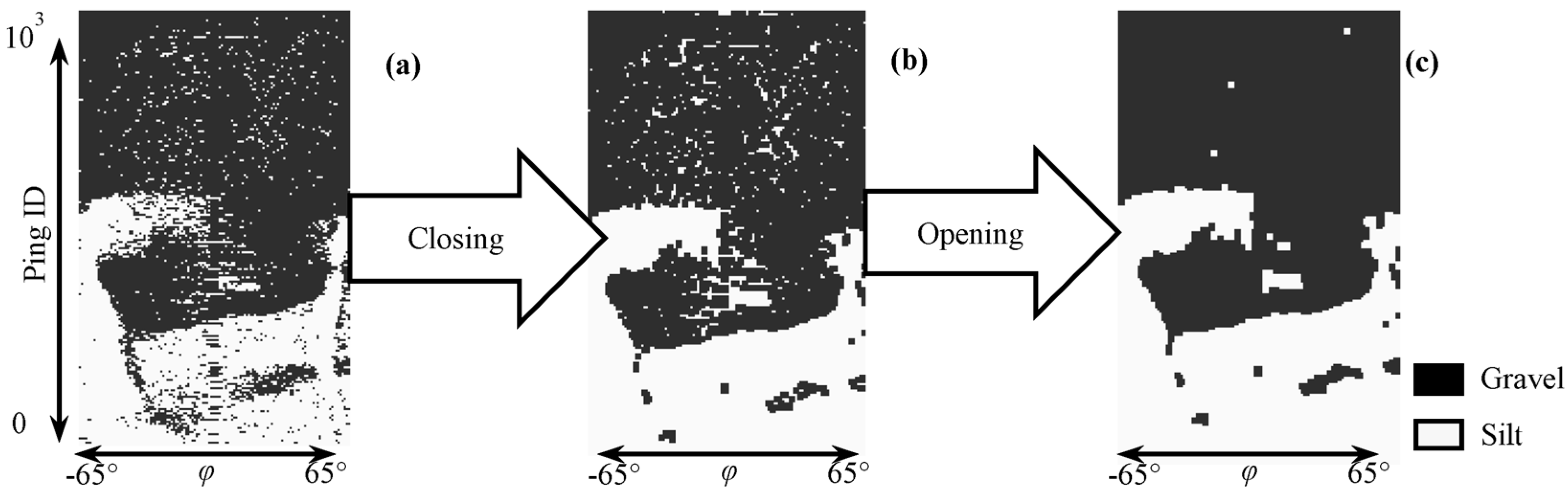
Figure 6.
Acquisition of SSS sediment image. (a) Raw SSS waterfall image; (b) angular image; (c) normalized image; (d) sediment image; and (e) denoised sediment image. φ is the incident angle.
Figure 6.
Acquisition of SSS sediment image. (a) Raw SSS waterfall image; (b) angular image; (c) normalized image; (d) sediment image; and (e) denoised sediment image. φ is the incident angle.

Figure 7.
Image transformation using thin plate spline (TPS). The red dot in the figure is the reference point. (a) raw image; (b) transformed image.
Figure 7.
Image transformation using thin plate spline (TPS). The red dot in the figure is the reference point. (a) raw image; (b) transformed image.

Figure 8.
Superimposition of the corrected SSS image and MBES sounding terrain.
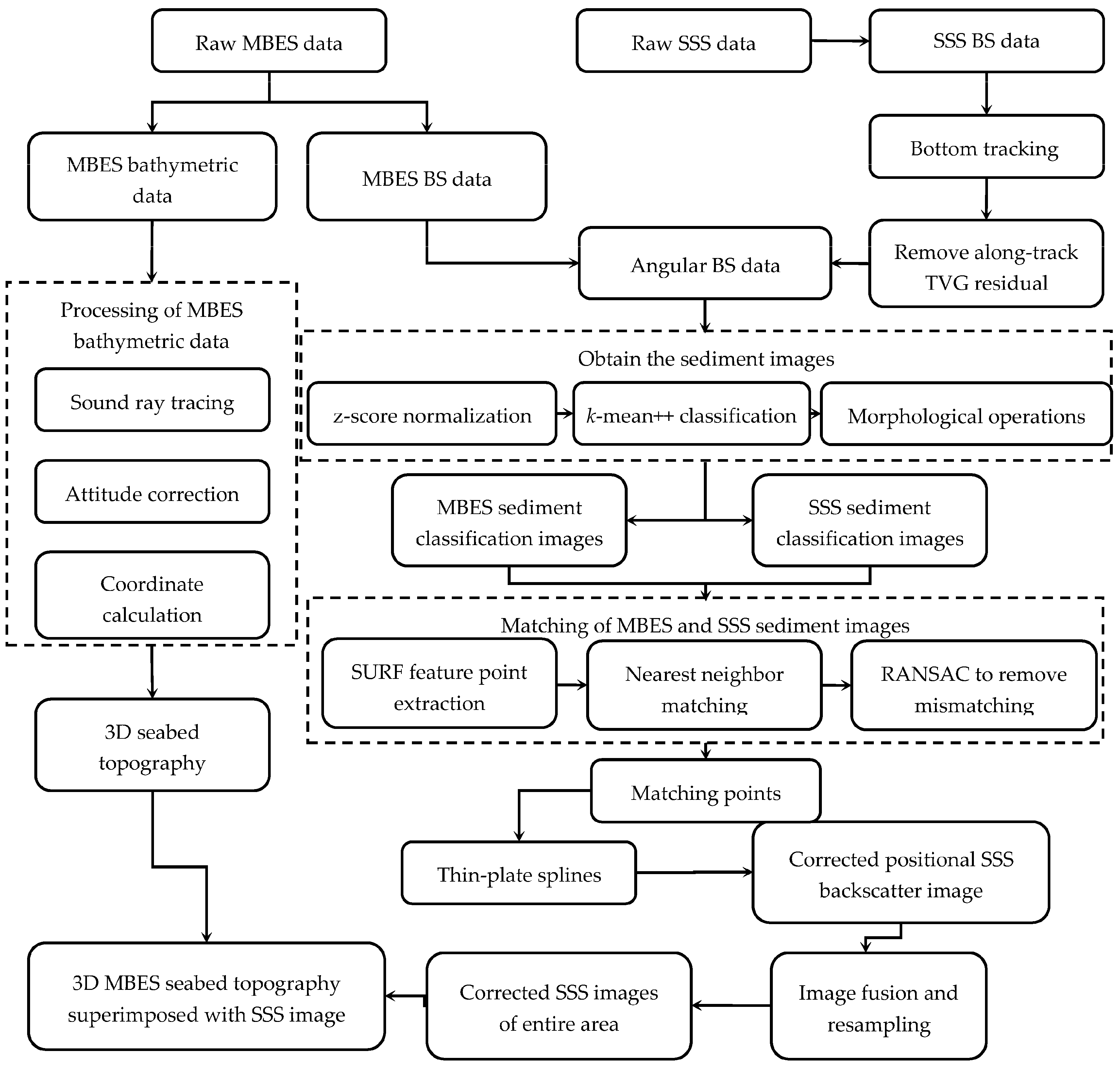
Figure 9.
(a) Tracks of MBES and SSS survey lines in the measurement area; (b) digital elevation model (DEM) established by MBES sounding data; (c,d) the geocoded MBES snippet and SSS images.
Figure 9.
(a) Tracks of MBES and SSS survey lines in the measurement area; (b) digital elevation model (DEM) established by MBES sounding data; (c,d) the geocoded MBES snippet and SSS images.
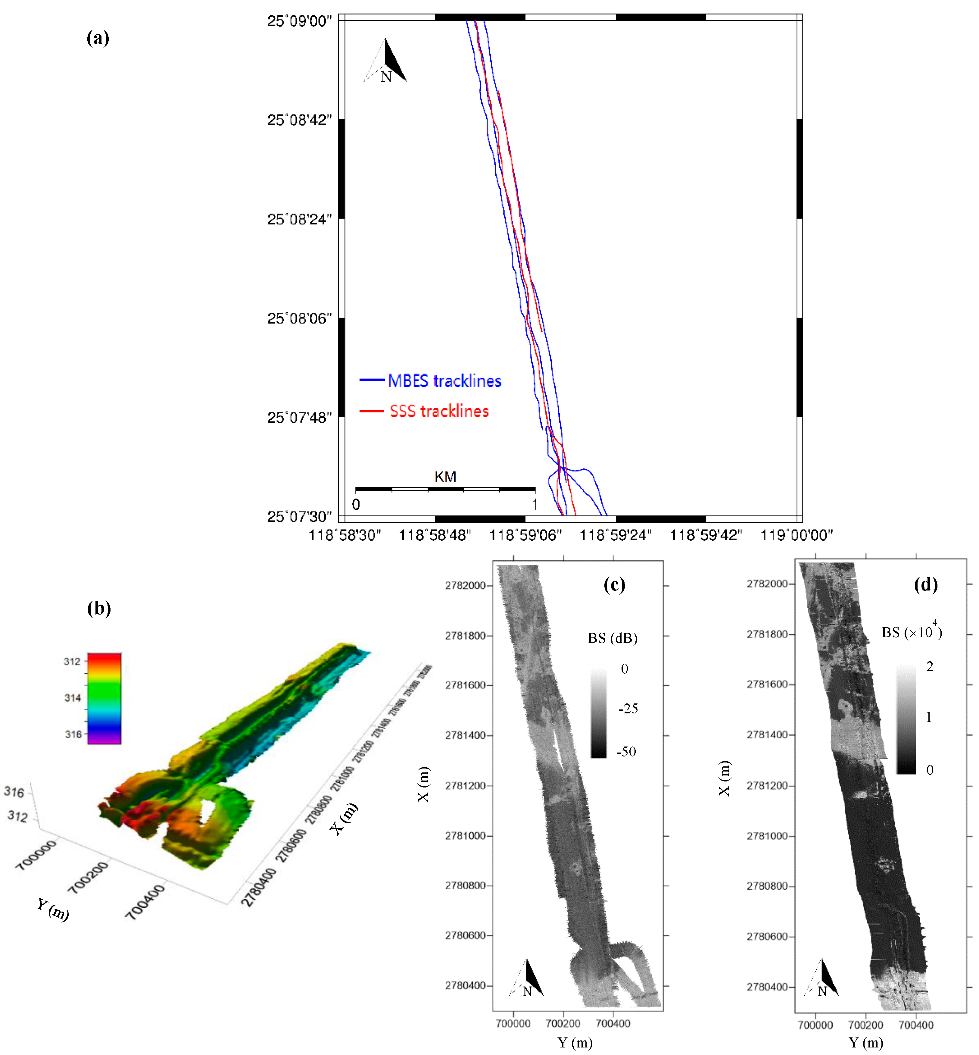
Figure 10.
Segmental matching of MBES and SSS images. (a) SSS waterfall image; (b) transformed angular image from (a); (c) normalized image of (b); (d) SSS sediment image; (e) denoised image of (d); and (f) geocoded image of (e). (A) MBES snippet waterfall image, (B) transformed angular image from (A), (C) normalized image, (D) MBES sediment image, (E) denoised sediment image, and (F) geocoding image of (E). (R1–R3) three segments divided from the MBES image according to the distributions of seabed sediments and targets. φ is the incident angle.

Figure 11.
Matching of MBES and SSS images and the corrected position SSS image in entire waters. (a) MBES radiometric corrected images; (b) raw SSS image; and (c) corrected position SSS images. All (a–c) are in the same region as Figure 9b.
Figure 11.
Matching of MBES and SSS images and the corrected position SSS image in entire waters. (a) MBES radiometric corrected images; (b) raw SSS image; and (c) corrected position SSS images. All (a–c) are in the same region as Figure 9b.
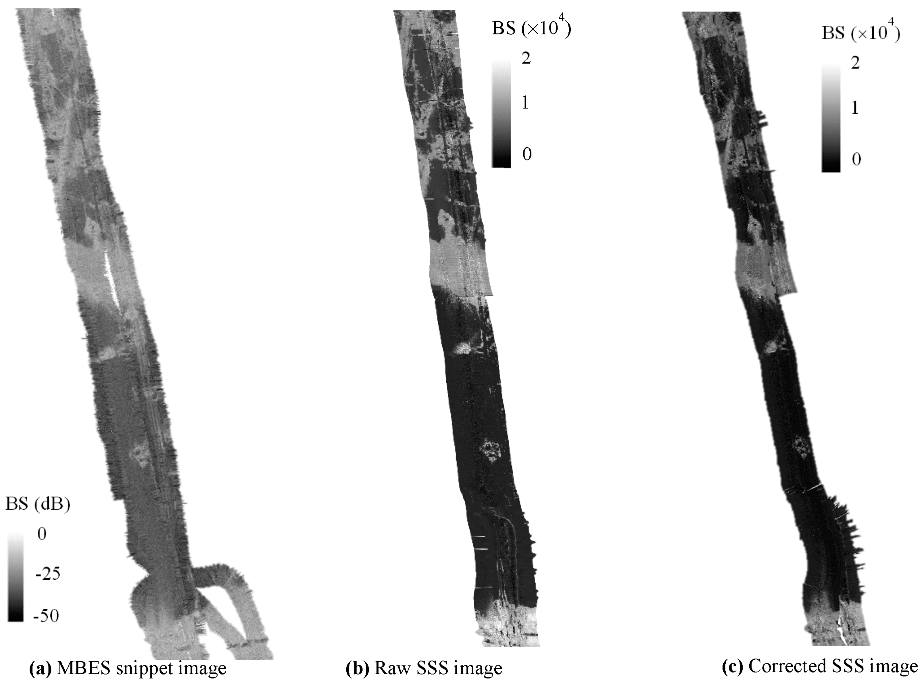
Figure 12.
Superimposition of the MBES snippet image and terrain (A) and that of the corrected positional SSS image and MBES terrain (B) in entire waters. (a–c) denote three small areas at different locations of the measurement area.
Figure 12.
Superimposition of the MBES snippet image and terrain (A) and that of the corrected positional SSS image and MBES terrain (B) in entire waters. (a–c) denote three small areas at different locations of the measurement area.

Figure 13.
Comparison of two types of superimpositions. (A,B) denote the superimposition shown in Figure 12, and (a–c) are the enlarged (a–c) shown in Figure 12.
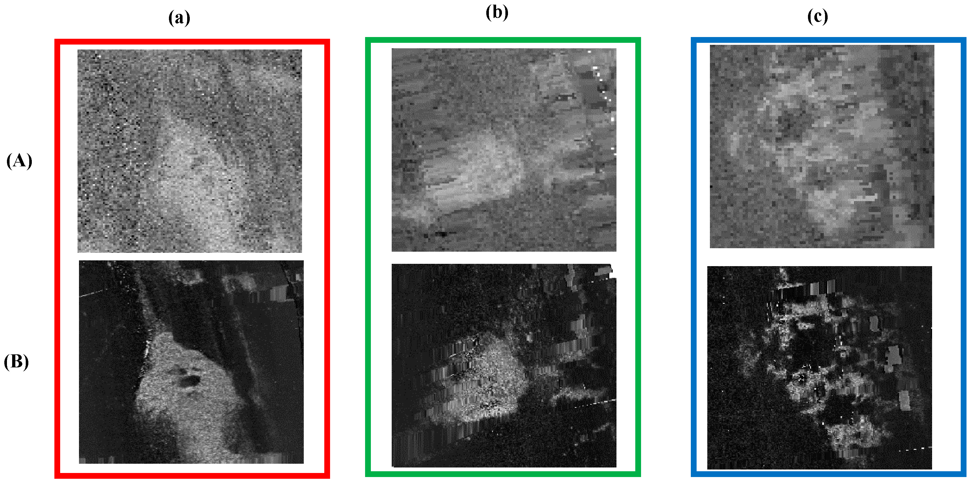
Figure 14.
Comparison of the wrapped images using the TPS and the rigid transform. (a) Raw SSS image; and (b,c) corrected images using the TPS and rigid transformation, respectively. The blue and red points denote the feature points in the SSS image and the MBES image.
Figure 14.
Comparison of the wrapped images using the TPS and the rigid transform. (a) Raw SSS image; and (b,c) corrected images using the TPS and rigid transformation, respectively. The blue and red points denote the feature points in the SSS image and the MBES image.
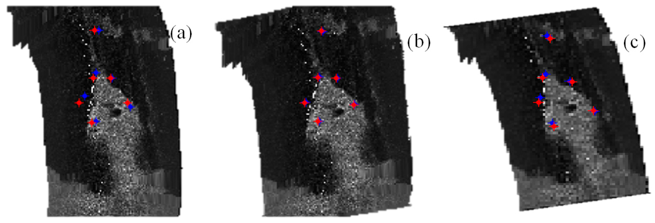
Figure 15.
Positional errors of entire feature points of the raw SSS image and SSS images corrected using the rigid transform and TPS, respectively.
Figure 15.
Positional errors of entire feature points of the raw SSS image and SSS images corrected using the rigid transform and TPS, respectively.

Figure 16.
Statistical curves of the MBES and SSS BSs of the silt sediment.


Table 1.
Statistical parameters of positional errors of entire feature points in the raw SSS image and SSS images corrected using the rigid transform and TPS, respectively.
Table 1.
Statistical parameters of positional errors of entire feature points in the raw SSS image and SSS images corrected using the rigid transform and TPS, respectively.
| Max Deviation (m) | Mean Deviation (m) | Standard Deviation (±m) | |
|---|---|---|---|
| Raw data | 23.00 | 9.11 | 11.87 |
| Rigid transformation | 15.00 | 3.33 | 3.80 |
| TPS | 6.00 | 2.50 | 0.67 |
© 2017 by the authors. Licensee MDPI, Basel, Switzerland. This article is an open access article distributed under the terms and conditions of the Creative Commons Attribution (CC BY) license (http://creativecommons.org/licenses/by/4.0/).
Share and Cite
MDPI and ACS Style
Zhao, J.; Meng, J.; Zhang, H.; Yan, J. A New Method for Acquisition of High-Resolution Seabed Topography by Matching Seabed Classification Images. Remote Sens. 2017, 9, 1214. https://doi.org/10.3390/rs9121214
AMA Style
Zhao J, Meng J, Zhang H, Yan J. A New Method for Acquisition of High-Resolution Seabed Topography by Matching Seabed Classification Images. Remote Sensing. 2017; 9(12):1214. https://doi.org/10.3390/rs9121214
Chicago/Turabian StyleZhao, Jianhu, Junxia Meng, Hongmei Zhang, and Jun Yan. 2017. "A New Method for Acquisition of High-Resolution Seabed Topography by Matching Seabed Classification Images" Remote Sensing 9, no. 12: 1214. https://doi.org/10.3390/rs9121214
Note that from the first issue of 2016, this journal uses article numbers instead of page numbers. See further details here.