Article

Estimating Leaf Area Density of Individual Trees Using the Point Cloud Segmentation of Terrestrial LiDAR Data and a Voxel-Based Model

1
School of Resources and Environment, University of Electronic Science and Technology of China, No. 2006, Xiyuan Ave, West Hi-Tech Zone, Chengdu 611731, China
2
Center for Information Geoscience, University of Electronic Science and Technology of China, No. 2006, Xiyuan Ave, West Hi-Tech Zone, Chengdu 611731, China
3
Department of Surveying and Mapping Engineering, Sichuan Water Conservancy Vocational College, Chongzhou 611231, China
4
Department of Geography, Planning, and Environment, East Carolina University, Greenville, NC 27858, USA
*
Author to whom correspondence should be addressed.
Remote Sens. 2017, 9(11), 1202; https://doi.org/10.3390/rs9111202
Submission received: 19 September 2017 / Revised: 19 November 2017 / Accepted: 20 November 2017 / Published: 22 November 2017

Abstract

:
The leaf area density (LAD) within a tree canopy is very important for the understanding and modeling of photosynthetic studies of the tree. Terrestrial light detection and ranging (LiDAR) has been applied to obtain the three-dimensional structural properties of vegetation and estimate the LAD. However, there is concern about the efficiency of available approaches. Thus, the objective of this study was to develop an effective means for the LAD estimation of the canopy of individual magnolia trees using high-resolution terrestrial LiDAR data. The normal difference method based on the differences in the structures of the leaf and non-leaf components of trees was proposed and used to segment leaf point clouds. The vertical LAD profiles were estimated using the voxel-based canopy profiling (VCP) model. The influence of voxel size on the LAD estimation was analyzed. The leaf point cloud’s extraction accuracy for two magnolia trees was 86.53% and 84.63%, respectively. Compared with the ground measured leaf area index (LAI), the retrieved accuracy was 99.9% and 90.7%, respectively. The LAD (as well as LAI) was highly sensitive to the voxel size. The spatial resolution of point clouds should be the appropriate estimator for the voxel size in the VCP model.

Graphical Abstract

1. Introduction

Foliage plays an important role in the energy budget through photosynthesis, transpiration, respiration, and the maintenance of the plant microclimate [1]. The spatial distribution of leaves is critical for describing the transmission and interception of solar radiation for wood production, species competition, ecosystem dynamics, and biodiversity [2]. The leaf area index (LAI) is generally used for expressing the amount of leaves in a tree canopy, and has been successfully retrieved by using remotely sensed data at different scales [3]. The determination of LAI is common. However, LAI can be difficult to use for characterizing the structure of a heterogeneous canopy, and may be less effective or more complicated to use in cases where leaves have irregular shapes and forms [2,4].
As one of the canopy vertical structure parameters, the leaf area density (LAD) in each horizontal layer is generally used for the quantification of the leaves in the canopy [2]. LAD is defined as the total one-sided leaf area per unit volume [5]. Integrating the LAD profile data vertically, one can calculate the LAI [6]. LAD can be estimated in situ using direct, semi-direct, or indirect approaches [2]. The direct method involves the counting and measurement of leaves, but this application is limited, because it is destructive and time consuming. One of the representative semi-direct methods is Wilson’s inclined point quadrat method, which counts the number of contacts of a leaf with probes inserted into the vegetation canopy [7]. Indirect techniques mainly involve the use of passive optical devices based on a gap fraction method, such as hemispherical photography, which relies on the Beer–Lambert law of light transmission through a turbid medium adapted to canopies [8]. However, these methods are limited in the spatial explicitness of their estimates, as well as in their accuracy [2,5].
Light detection and ranging (LiDAR) sensors have recently been applied to obtain the three-dimensional (3D) structural properties of plants [9,10,11,12]. A terrestrial LiDAR sensor emitting small-footprint laser pulses at a high pulse repetitive frequency and with small angular steps between consecutive pulses provides a fine spatial resolution, which allows the inner canopies of trees to be assessed from the ground and makes the accurate estimation of LAD profiles possible [1,13]. One of the important prerequisites in the estimation of canopy LAD is the ability to describe the spatial distribution of leaves separately from that of wood, because the point clouds include not only leaves, but also non-leaf components (such as twigs, branches, and the stem/trunk) of the plant, which will affect the estimation accuracy of LAD [13]. The LAD estimation is greatly affected by whether the leaf and non-leaf components are well separated in the point clouds. Hosoi and Omasa showed that the LAD of Zelkova serrata was overestimated by 19% if the LiDAR points of the woody components were not eliminated [6]. To classify leaf and non-leaf components in a laser point cloud, many studies have used manual techniques, where laser points associated with different canopy components are visually identified [1,6]. However, these methods are labor intensive and time consuming, which limits the use of LiDAR data at relatively broad spatial scales for estimating LAD [14]. Distinguishing a leaf from a trunk or branch by using the intensity of the reflected pulse relies on the differences in their optical properties at the wavelength of the LiDAR sensor [2,15]. However, the laser return intensity is affected by the distance and incidence angle. The radiometric calibration of the intensity is not easy [14]. The geometric method was also used to separate the photosynthetic and non-photosynthetic components in the terrestrial LiDAR data of forest canopies [14,16]. Unfortunately, the geometric information is not easy to obtain, either. The reflectance values associated with a digital camera can be useful for automatically classifying the structural parameters of the canopy [17]. However, the dimensionless and uncalibrated reflectance values are highly variable [14]. In recent years, a non-destructive and rapid object extraction method called point cloud segmentation has been used for ground object extraction and classification from airborne LiDAR data [18,19,20,21]. However, the segmentation method has been seldom used to extract leaf point clouds using high-resolution terrestrial LiDAR data. The leaf is significantly different from the other parts of the tree, such as the stem and trunk, both in shape and size. Consequently, the segmentation of high density unorganized 3D LiDAR point clouds should have the potential to distinguish leaves from the other parts of the tree.
Recently, many researchers have attempted to develop various models for the estimation of LAD using LiDAR sensors [1,15,22,23,24]. Among the models, the voxel-based method has been commonly used for describing the computation of a 3D matrix of voxels from terrestrial LiDAR point clouds. The method has the characteristic that no assumption about the spatial distribution, size, or shape of canopy components is made. This method is also easy to operate. The vegetation density of a voxel can be computed using the number of echoes inside the voxel [25]. The voxel-based method has been successfully used in individual trees and woody canopy LAD estimation [2,4,13,15,25,26,27,28]. Hosio and Omasa developed a voxel-based canopy profiling (VCP) method to express the laser trace information as a voxel that serves as an attribute of a 3D array [1]. Based on each voxel, both LAD profiles and the LAI of an individual tree can be accurately estimated by counting the frequency of contact between laser beams and the foliage of the canopy in each horizontal layer. The same group of researchers applied this method to a natural forest stand [6] and woody materials [11,26]. Wang et al. estimated the LAD of a magnolia canopy using the VCP method based on terrestrial LiDAR and true color images [17]. Therefore, the voxel-based method is a promising way to estimate LAD. However, the voxel size needs to be chosen carefully, because it can significantly influence the estimation accuracy of the LAD [2]. The calculation accuracy and efficiency depend on the voxel size. An assessment of the effect of the voxel size on the LAD estimation model is needed. The objectives of this study are: (1) to develop an effective workflow to estimate LAD for individual magnolia trees on the basis of high-resolution terrestrial LiDAR measurements; (2) to propose a point cloud segmentation method for leaf extraction; and (3) to quantify the impact of voxel size on the LAD estimations for individual trees.

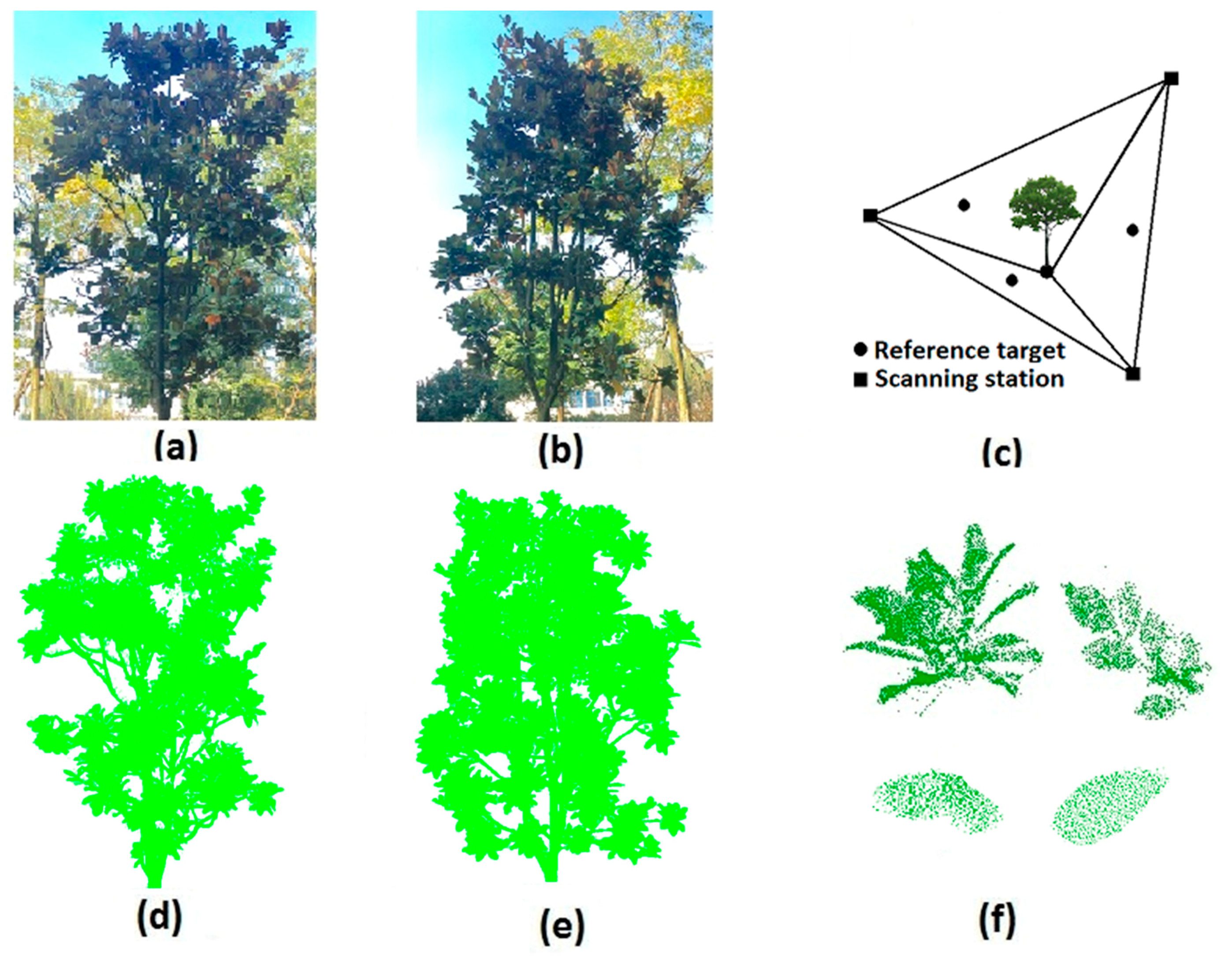
2. Study Site and Field Measurements

The study site was located on the campus of University of Electronic Science and Technology of China, Chengdu, Sichuan, China. The ground area was almost flat. For this study, two individual magnolia trees (Table 1 and Figure 1) were selected and scanned with Leica ScanStation C10, which has a full 360° × 270° field of view, long range (300 m@90% reflectivity), and high scan frequency (50,000 points/s). The laser wavelength is 532 nm.
The tree was scanned from three scan locations, and three reference targets were placed on the ground to establish correspondences between different scanning stations (Figure 1c). For all of the scans, ScanStation C10 was placed on a survey tripod approximately 1.5 m above the ground, and at a distance of about 5–8 m from the tree to ensure that the entire crown was well within the view window. The scans were all performed under very low wind conditions. The high scanning resolution or point spacing for every site was approximately 0.05 m at a distance of 100 m, because this scanning resolution was sufficient to identify a small leaf. More than 600 points exist on one leaf on average, and the mean point spacing (spatial resolution) is approximately 2.5 mm (Figure 1f).
Point clouds from the three scan locations with their individual coordinate systems were registered into one point cloud dataset under a common coordinate system using Leica Cyclone v9.1® and an improved iterative closest point algorithm based on k-dimensional tree [29,30]. The registration error was within 2 mm.

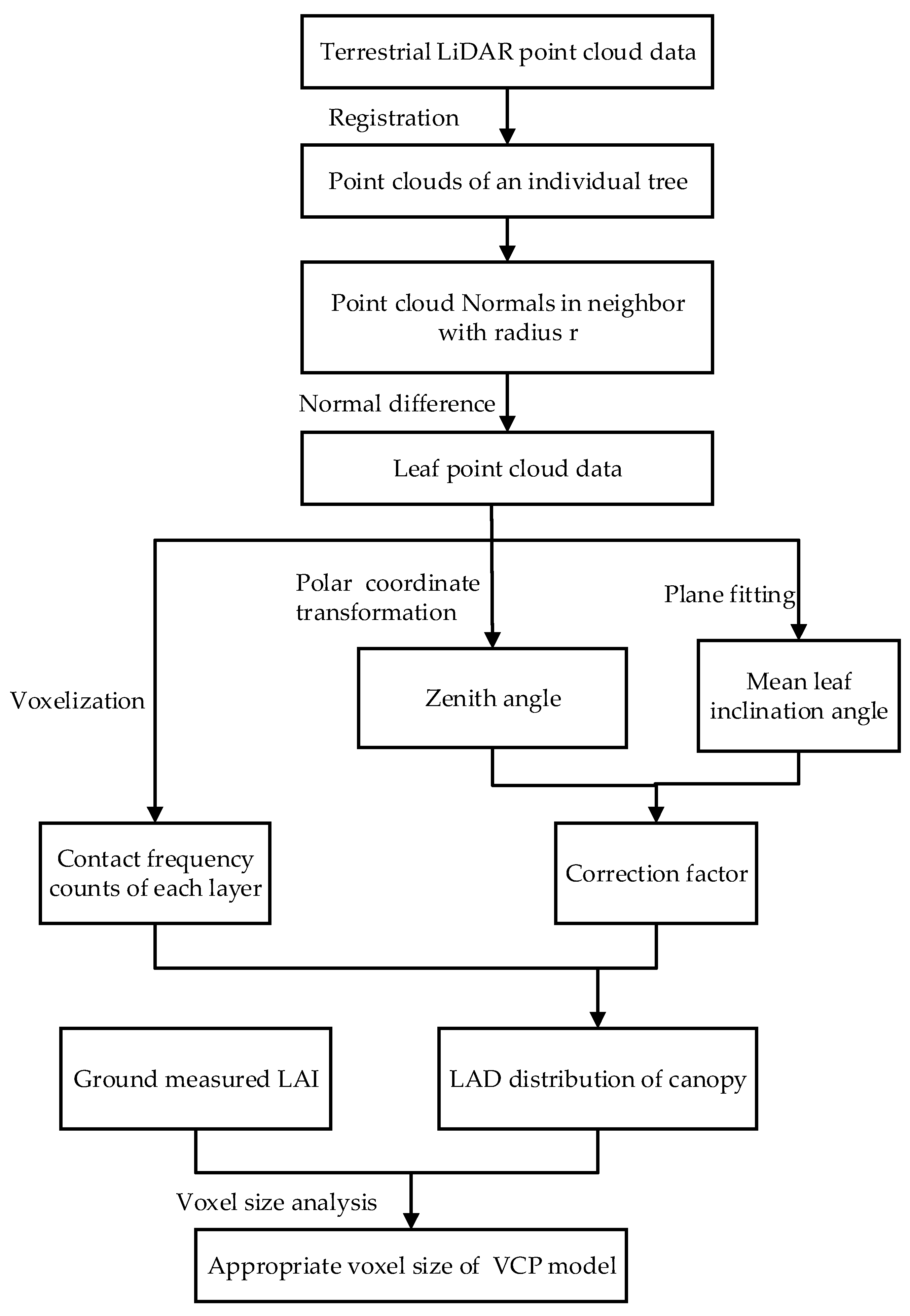
3. Materials and Methods

Figure 2 illustrates the developed LAD estimation workflow, which consists of leaf point cloud extraction and LAD estimation. Details are presented next.

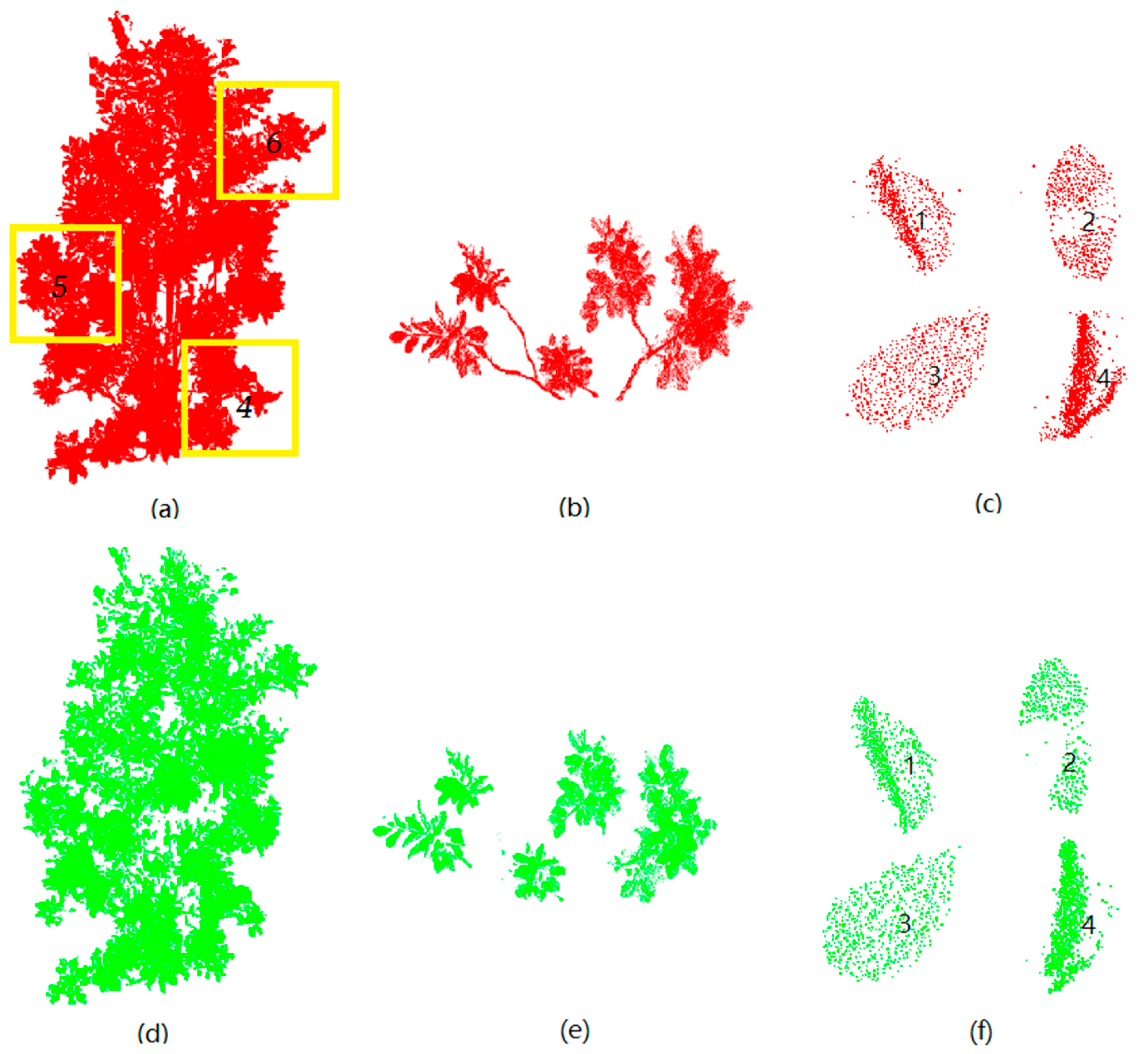
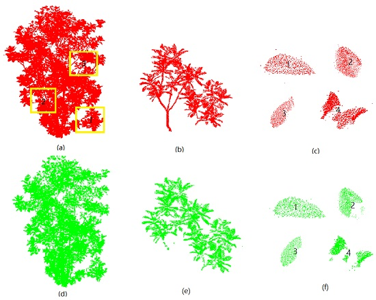
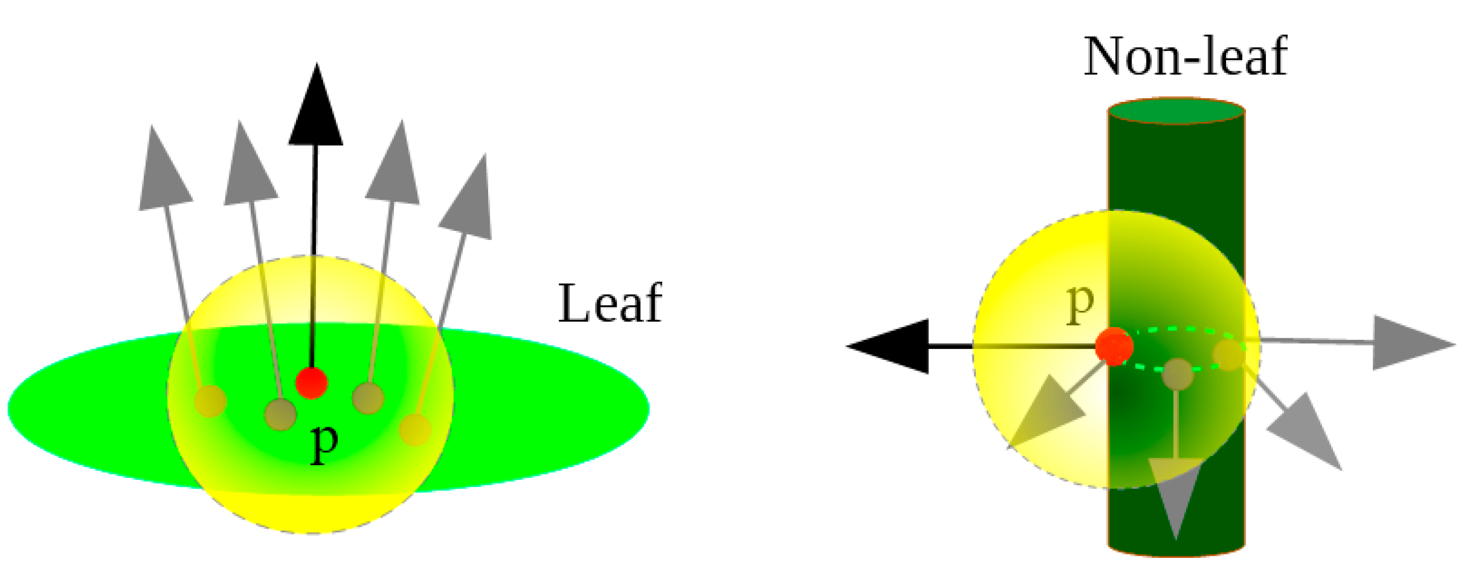
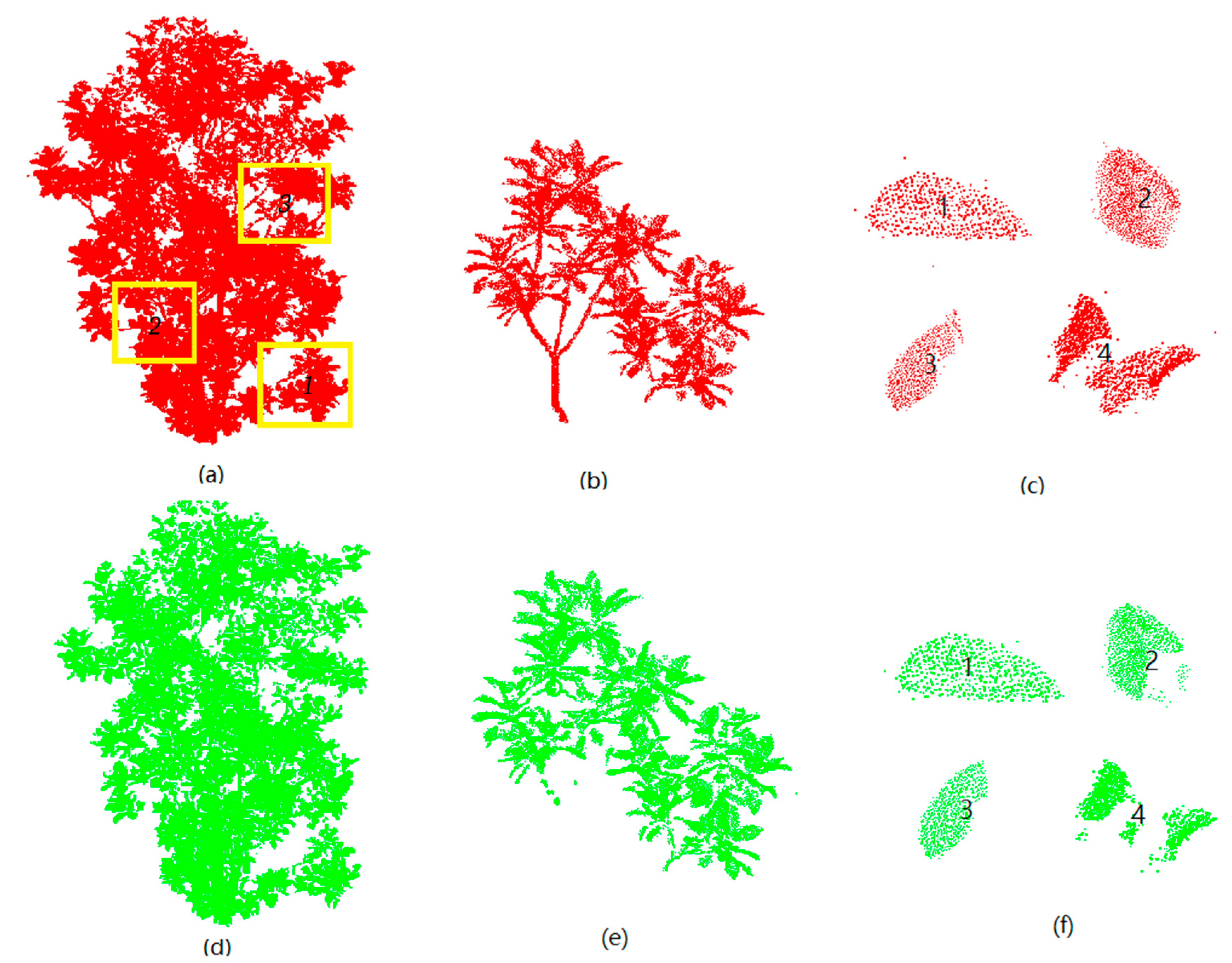
3.1. Extraction of Leaf Point Cloud

In the segmentation of point clouds, a point is partitioned into subregions to extract important features from the cloud data. The segmentation methods can be roughly classified into three categories: edge-detection, region-growth, and hybrid methods. The edge-detection methods detect discontinuities in the surfaces that form the closed boundaries of components in the point data. The region-growth methods detect continuous surfaces that are homogeneous or similar in geometrical properties. The hybrid approaches combine the edge-detection and region-based methods [31].
The normal of the point cloud is a very important characteristic parameter for unorganized 3D point cloud segmentation. If the direction of the two normals is almost identical, the surface structure does not change significantly. If the structure around a center point is significantly different from the other points, the direction of the two estimated normals is likely to vary by a relatively large margin [18]. Since most of the magnolia leaf surfaces are nearly flat, the normal vectors of these point clouds have similar directions. The non-leaf parts are composed from cylindrical segments. The point clouds of the non-leaf components located on the cylindrical surface and the normal vector of these point clouds have different directions (Figure 3). The normal difference of the leaf point cloud is generally smaller than that of the non-leaf component in the neighborhood. The normal difference method was proposed to segment leaf point clouds, which counts the normal difference between each point and the other points in the neighborhood.
There are many methods for estimating the normals of point clouds. However, only those using a fixed support radius or a fixed number of neighbors are suitable for point clouds. The normals were estimated by finding the tangent plane and using the principal components of a local neighborhood of fixed support radius around each point [18]. For point pi in the point cloud P, the normal difference operator in the neighbors are determined by
Δ n ^ ( p , r ) = 1 N i = 1 N ( n ^ ( p ) n ^ ( p i ) )
where n ^ (p) is the normal vector of point p in the neighbors, while radius r is the average spatial distance between two leaves.   n ^ ( p i ) is the normal vector of point pi. Δ n ^ ( p , r ) is the normal difference operator. The leaf point cloud is determined using the magnitude of Δ n ^ ( p , r ) as the threshold. The Otsu algorithm was applied to estimate the threshold [32]. The normal difference results of the point cloud data were viewed as the grey values of images. The appropriate threshold value was calculated through iteration to ensure the maximum variance between the leaf point cloud (foreground) and the non-leaf point cloud (background), as well as the minimal classification error.
Three cubes were chosen to manually evaluate the segmentation accuracy in the upper, middle, and bottom of the canopy, respectively. The non-leaf components were manually deleted. Then, the point number was counted. The leaves’ extraction accuracy was calculated from the ratio of the number of segmented leaf points to the number of manually classified leaf points. The overall segmentation accuracy was the average accuracy values of three test cubes.

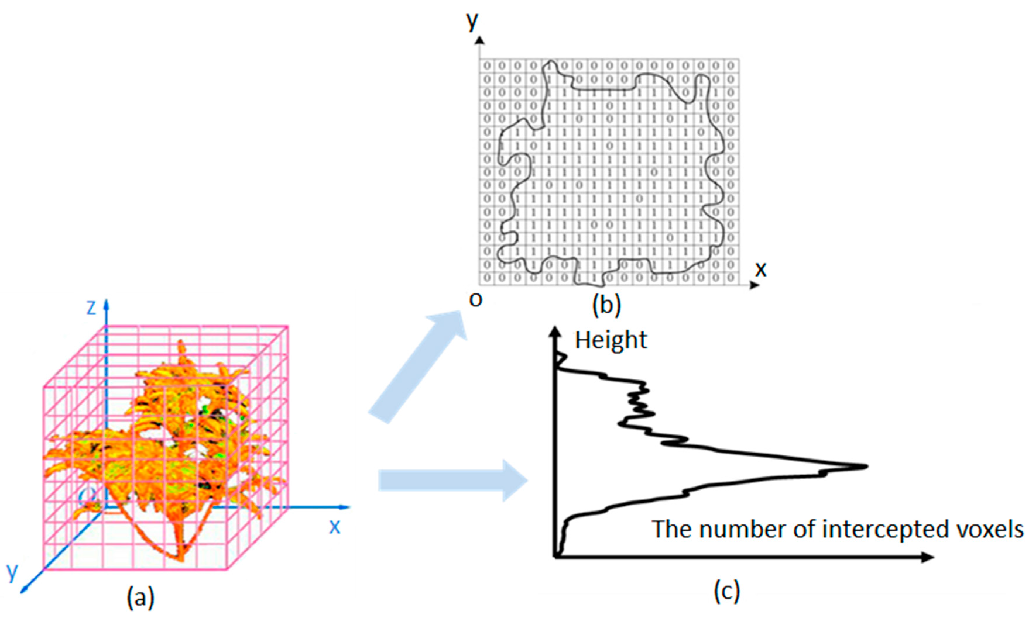
3.2. Voxel-Based LAD Estimation Method
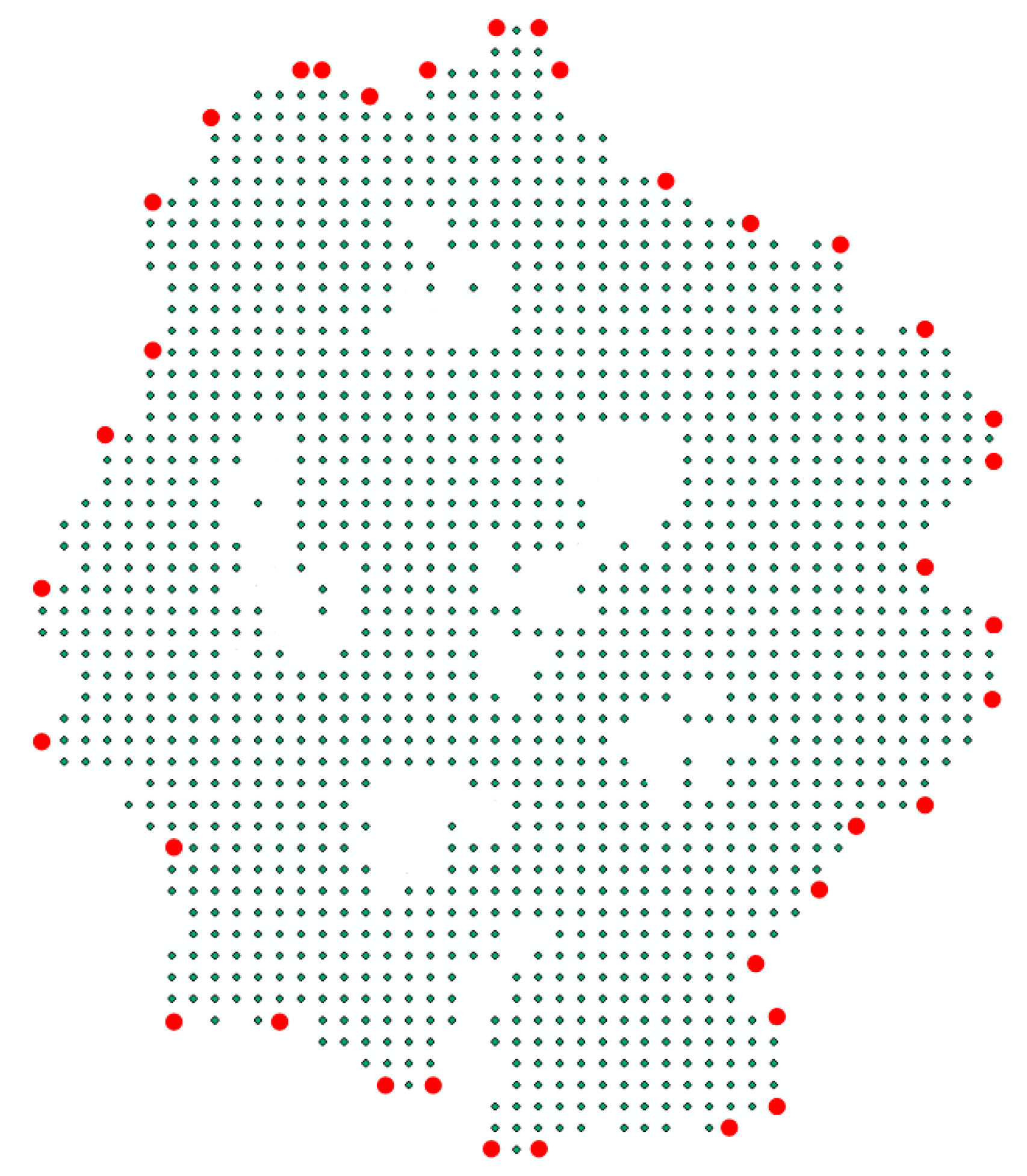
The voxel-based LAD estimation method mainly includes the voxelization and computation of the contact frequency of the laser beams in each horizontal layer [1].

3.2.1. Voxelization

A bounding box is first constructed to represent the domain of the registered leaf point clouds. The boundaries of voxel coordinates are determined by the minimum and maximum values of X, Y, and Z coordinates from the Cartesian coordinates of the point cloud region. During voxelization, a voxel is defined as a volume element in a 3D array. The range and scan resolution of the LiDAR determine the voxel size, which was set to 2.5 mm in this study. With the voxelization method, the registered leaf point cloud datasets can be grouped into individual voxels [1]. Therefore, voxelization reduces the number of points in a cloud, and improves the computational efficiency of the point cloud contact frequency. Defining the width (w), length (l), and height (h) for each voxel, we grouped the point clouds into Nl × Nw × Nh voxels, where Nl = (Xmax − Xmin)/l, Nw = (Ymax − Ymin)/w, and Nh = (Zmax − Zmin)/h [3]. In addition, the voxel coordinates can be calculated as
{ i = X min + ( int ( X X min ) / l ) × l j = Y min + ( int ( Y Y min ) / w ) × w k = Z min + ( int ( Z Z min ) / h ) × h
where (i, j, k) denote the voxel coordinates in the voxel array. Int is an integer operator. (X, Y, Z) represent the point coordinates of the registered LiDAR point data [1]. The voxel attribute determines the presence of a laser point in the voxel. A voxel with attribute 1 implies that the laser beam is intercepted inside the voxel. A voxel with attribute 0 indicates that there was no interception of the laser beam inside the voxel [1]. The attribute assignment of voxels within a horizontal layer, and a schematic map of the voxel-based model, are shown in Figure 4.

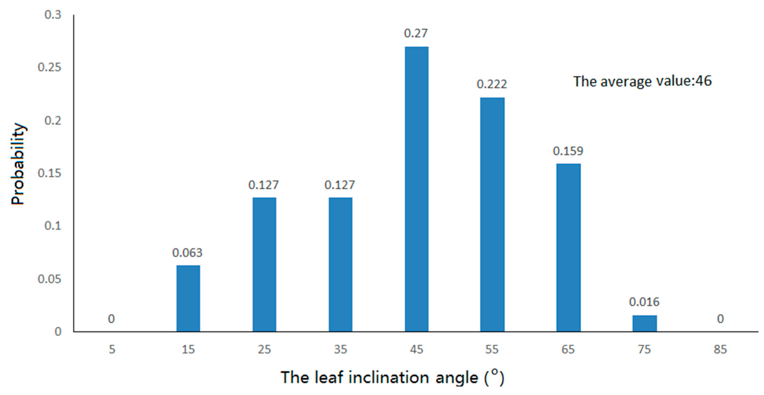
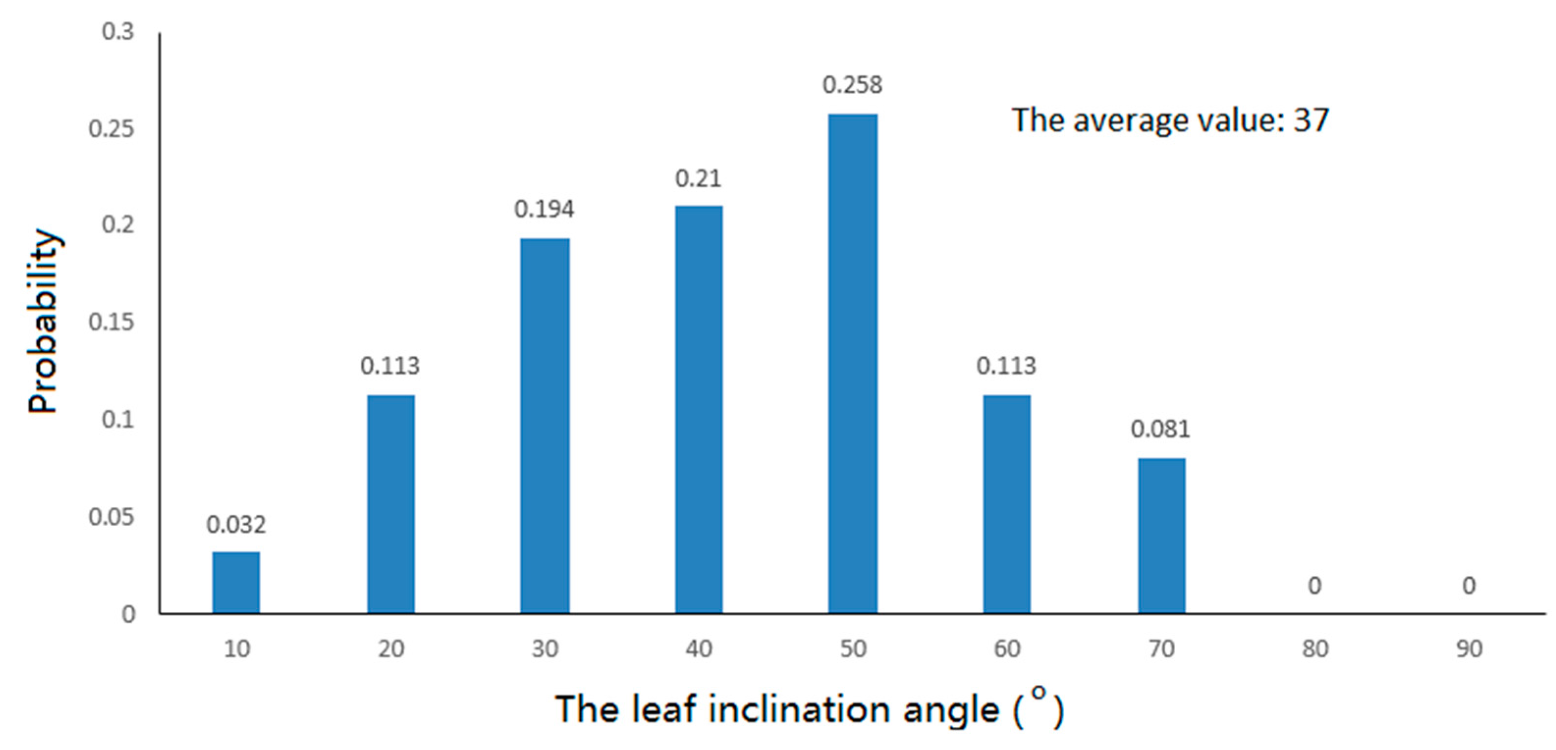
3.2.2. LAD Estimation Model Description
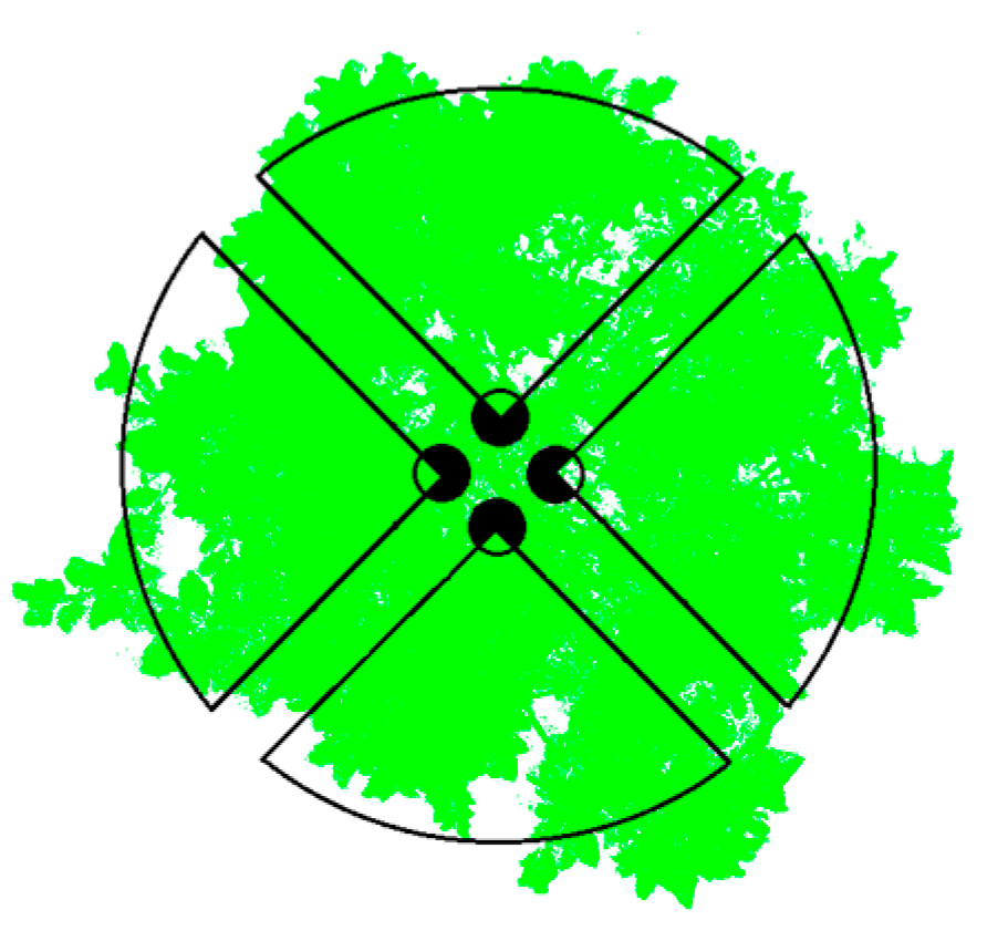
In the LAD computation, a plant region defined as the region above an area covered by a projection of the canopy on the horizontal plane was set in a voxel array. The area covered by the projection of the canopy was produced in the array by projecting all of the voxels with attribute 1 onto the horizontal plane at k = 0. Voxels above the area were regarded as voxels within the plant region, and used for the LAD computation. Thus, LAD was calculated in each horizontal layer of the canopy using the voxel-based canopy profiling (VCP) method [1,6]. In particular, LAD(h, ∆H), which is the LAD between heights h and h + ∆H above the ground, can be calculated as [1,6]
LAD ( h , Δ H ) = α ( θ ) 1 Δ H k = m h m h + Δ H n l ( k ) n l ( k ) + n p ( k )
where θ denotes the zenith angle of a laser beam; ∆H represents the horizontal layer thickness (0.5 m in this study); mh and mh + ∆H indicate the voxel coordinates on the vertical axis equivalent to height h and h + ∆H in orthogonal coordinates (h = ∆k × mh); and   n l ( k ) and n P ( k ) denote the numbers of voxels with the attribute values of 1 and 0 in the k-th horizontal layer of the voxel array, respectively. Thus, ( n l ( k ) + n P ( k ) ) is the total number of incident laser beams that reach the k-th layer. n l ( k ) is obtained by counting the number of voxels with attribute 1 in the k-th layer of the voxel-based tree model. n P ( k ) is obtained by counting the number of voxels with attribute 0 in the k-th layer. α(θ) is defined as
α ( θ ) = cos θ G ( θ )
which represents a correction factor that affects the leaf inclination angle at the laser incident zenith angle of θ. G(θ) stands for the mean projection of a unit leaf area on a plane perpendicular to the direction of the laser beam. G(θ) determined with the assumption that leaves are azimuthally symmetrical is
G ( θ ) = 1 2 π 0 2 π 0 π / 2 g ( θ L ) | cos ( n B , n L ) | d θ L d φ L = 0 π / 2 g ( θ L ) S ( θ , θ L ) d θ L
with
S ( θ , θ L ) = { cos θ cos θ L ,   for   θ π 2 θ L cos θ cos θ L [ 1 + 2 ( tan x x ) π ] ,   for   θ > π 2 θ L
x = cos 1 ( cot θ cot θ L )
where θ L   denotes the leaf inclination angle; φ L is the azimuth angle of the normal to the leaf surface; and n B   =   ( sin θ cos θ cos φ ,   sin θ sin φ ,   cos θ ) and n L   =   ( sin θ L cos θ L ,   sin θ L sin φ L ,   cos θ L ) are two unit vectors corresponding to the direction of the laser beam and the direction of the normal to the leaf surface, respectively. To use the field-measured distribution of leaf-inclination angles, one can rewrite Equation (5) as
G ( θ ) = q = 1 T q g ( q ) S ( θ , θ L ( q ) )
where q denotes the leaf inclination angle class, and Tq represents the total number of leaf inclination angle classes. Of each class, the range of the inclination angles is typically the same. Thus, if Tq = 18 is the number of leaf inclination angle classes existing from 0° to 90°, each class is 5° in range, or the interval is 5°. g ( q ) denotes the distribution of the leaf inclination angle for class q, which is the ratio of the leaf area belonging to class q to the total leaf area. θ L ( q ) stands for the midpoint angle of class q, which is the leaf inclination angle used for representing class q. With the eigenvalue method, leaves at different tree heights were randomly selected to fit the leaf planes and estimate the leaf inclination angles [1,6].
Contact frequency is calculated from the values of n l ( k ) and n P ( k ) in each horizontal thickness layer. Void voxels outside of the canopy exist because of the irregularity of the canopy structure and the 3D voxel model constructed using the maximum and the minimum coordinate values of the point cloud data. The voids should not be regarded as n P ( k ) , and are not used in the calculation for contact frequency. Thus, the canopy boundary determination and exclusion of invalid elements are important for the contact frequency calculation. Here, the simple and efficient two-dimensional convex hull algorithm, or Graham scan [33], is used to identify the canopy contour range in each horizontal layer. The algorithm can be described as follows. First, in one scan over the list of points, the point with the minimum y-coordinate is found and called p0. Next, the other points are sorted by their polar angle about the origin p0. If two points form the same angle with p0, then the one that is closer to p0 precedes the other in the ordering. Finally, starting from p0, the sorted points are sequentially scanned. If these points are on the convex hull polygon, each of the three successive points pi−1, pi, pi+1 should satisfy the following properties: pi+1 is located the left side of the vector <pi−1, pi>. If the properties are not met, pi must not be the apex on the convex hull, and should be deleted [34].

3.3. Validation

The validation method of LAD can be divided into a direct method and an indirect method. A direct method collects leaves hierarchically, and then measures the single leaf area of each layer. The workload of the method is heavy, and the method is destructive. It is almost important (to use the method) if trees are tall and study areas are large. An indirect method measures the LAI of the canopy by using LAI instrument. The sum of each layer’s LAD value of the total canopy height of h is called the canopy LAI. The relationship between LAD and LAI can be expressed as follows [35]
LAI   = 0 h LAD ( z ) dz
In the assessment of the estimated LAI, the LAI-2200™ instrument was chosen as validation data source provider. The LAI of a tree was measured using a 90° view cap, with the sensor placed near the base of the trunk (Figure 5). The view cap can prevent the sensor from seeing the trunk of the tree. LAI is computed by averaging the LAIs that are measured five times per tree.

3.4. Voxel Size Effects Analysis

Voxel size can influence the layer of detail of the structural information of the extracted canopy, and the computational accuracy of the contact frequency in the VCP model. Thus, voxel size is the key parameter for acquiring the structural information of the vegetation, and influences the LAD estimation accuracy. To understand the effect of the voxel size on the contact frequency, we use seven voxel sizes (2.5 mm, 5 mm, 10 mm, 25 mm, 50 mm, 62.5 mm, and 100 mm). The contact frequencies of each horizontal thickness layer (height interval = 0.5 m) for different voxel sizes will be calculated. The appropriate voxel size is analyzed based on measured LAI data.

4. Results and Discussion

4.1. Extraction of Leaf Point Cloud Data for Two Magnolia Trees
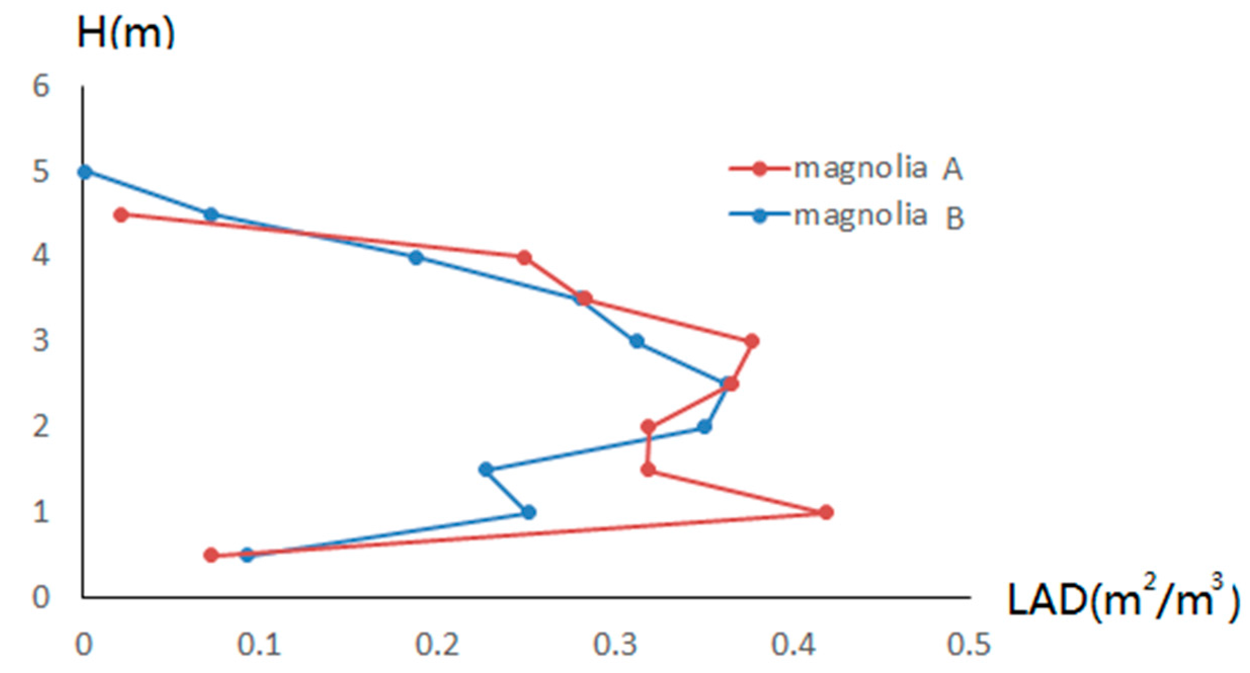
The average spacing of two leaves was 20 mm. Thus, the neighborhood radius was set up as 20 mm. The segmented leaf point clouds from Magnolia A, as shown in Figure 6d, were derived using the normal difference method. The segmentation threshold of 0.5 was chosen from the normal difference of the Otsu algorithm. Compared with the canopy’s original point clouds (Figure 6a), the majority of the points were related to leaves. To describe the segmentation results clearly, we showed the point clouds of cube 1 in Figure 6b. Segmented leaf point clouds based on the normal difference method of cube 1 are shown in Figure 6e. All of the leaves were successfully segmented. The obvious erroneous non-leaf parts that were segmented can be deleted manually, and the effect should be minimal. The number of all of the leaf point clouds extracted in test cube 1 (Figure 6e) was 98,042. The extraction accuracy was 86.84% in test cube 1. Similarly, the extraction accuracy levels of test cubes 2 and 3 were 87.22% and 85.54%, respectively. Therefore, the averaged accuracy level for Magnolia A was 86.53%. Close-up views of four leaves are shown in Figure 6c. The detailed segmented leaves’ point clouds are shown in Figure 6f. Noise points near the leaf were excluded. It indicated that all of the points located on leaf 1 and leaf 3 were segmented, but a few of the points on leaf 2 and leaf 4 were removed. These points were located on the curved surface of the leaves, and it is difficult to segment the points on a curly leaf since the normal directions of these points were different, and the normal differences of the curly leaf points were similar to the non-leaf components. A visual inspection of the leaves suggested that the shape and edges were kept well, although a few points were incorrectly eliminated.
Similarly, the leaf point clouds of Magnolia B (Figure 7) were extracted using the same steps and parameter settings (as Magnolia A). The leaves segmentation effects were similar with Magnolia A (Figure 7e,f). The accuracy of three test cubes were 83.23%, 82.81%, and 87.86%, respectively. The averaged accuracy value was 84.63%.

4.2. LAD Estimation

4.2.1. LAD Estimation in the Voxel Size of 2.5 mm

The canopy boundary contour in each horizontal layer was determined by the Graham scan algorithm using the location of the intercepted voxels. Figure 8 showed the outline of one horizontal layer that reflects the leaf coverage condition. The large red dots comprise the horizontal thickness of the boundary layer of the tree canopy.
Sixty leaves were randomly selected from each horizontal layer. The distribution probability of the leaf inclination angle was calculated using the probability of the leaf inclination angle at an interval of 10°, with the range from 0° to 90°. The inclination angle values of Magnolia A ranged between 15° and 75°, with a mean value of 46° (Figure 9). The inclination angle values of Magnolia B ranged between 10° and 70°, with a mean value of 37° (Figure 10). The mean zenith angle, correction coefficient, and contact frequency in each horizontal layer were calculated. The correction coefficients were mainly determined by mean zenith angle, and were near 1.10. The contact frequency distribution agreed with the leaves distribution. The maximum contact frequency of Magnolia A was 0.19, which occurred in layer 2. For Magnolia B, the maximum contact frequency was 0.17, which occurred in layer 5.
The vertical distribution of the LAD (Figure 11) was consistent with the vertical leaf distribution of the magnolia canopy (Figure 1). In each horizontal layer, the higher the leaf density, the larger the LAD. The maximum LAD of Magnolia A happened at 1.0 m of the canopy. Then, the LAD was positively related to height until 3.0 m. In the middle to higher layers of the canopy, the LAD of Magnolia A was inversely related to height. The LAD of Magnolia B at 1.0 m is much higher than 1.5 m. The LAD of Magnolia B reached the peak at 2.5 m, and then decreased gradually as the height continuously increased.
The cumulative LAD (LAI) was validated by the ground measured LAI (Table 2). The level of accuracy was 90.7% or higher.

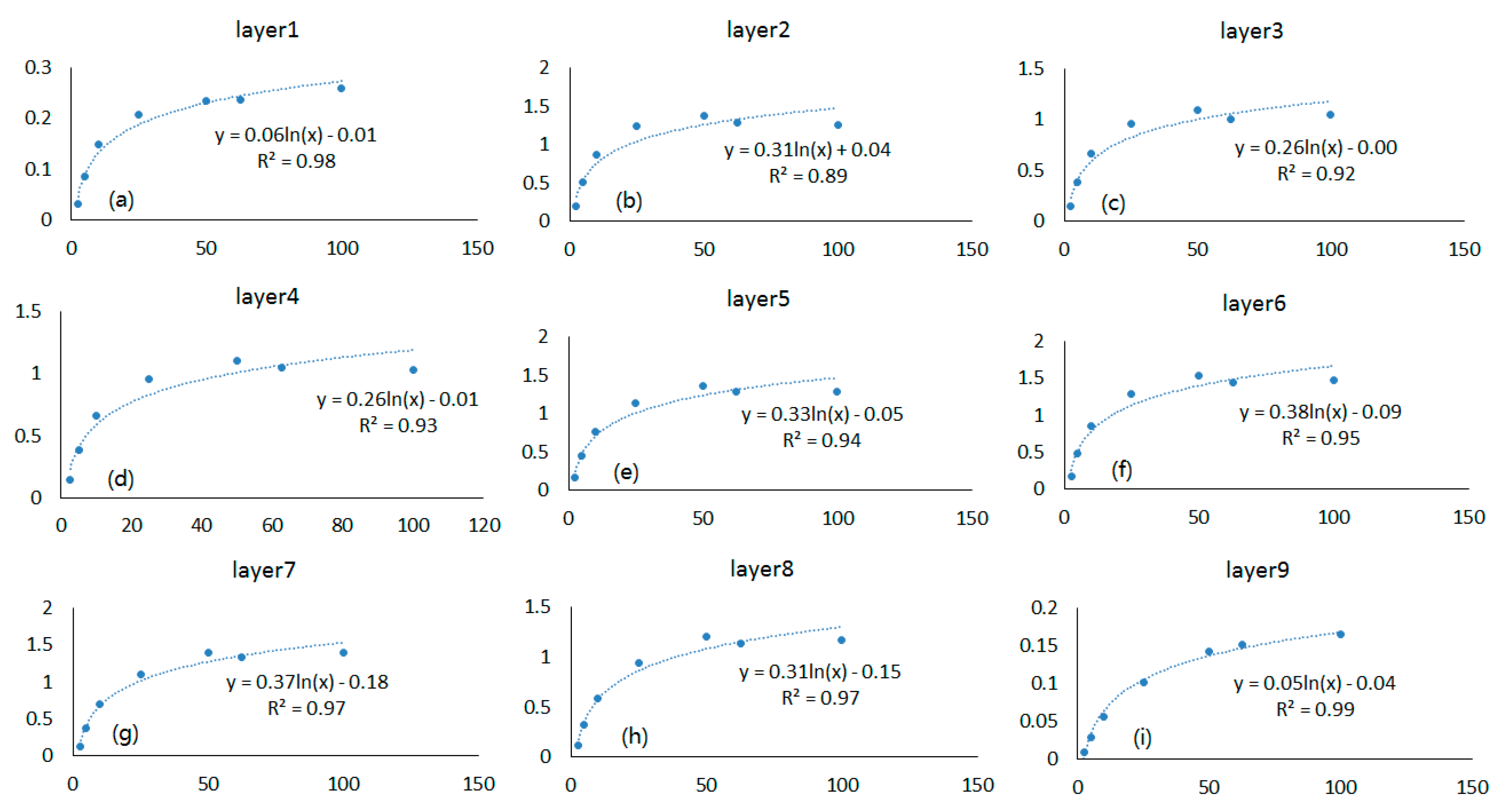
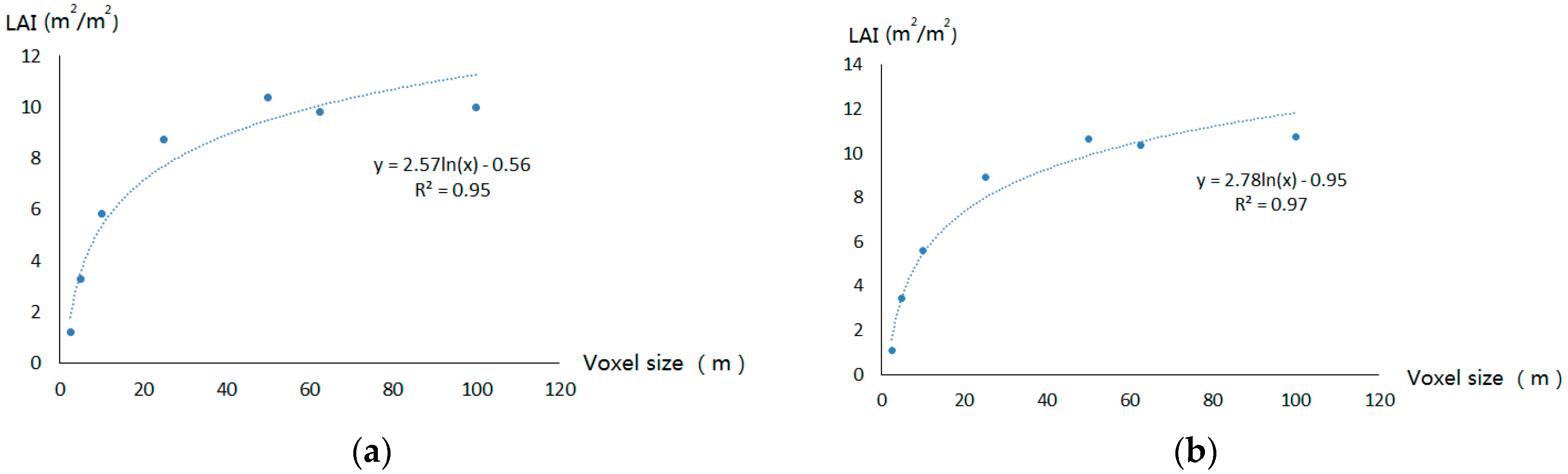
4.2.2. Voxel Size Effects

Variations in the contact frequency of different horizontal thickness layers for different voxel sizes are shown in Figure 12 in alphabetical order. It was clear that the contact frequency increased with an increase in the voxel size. They were highly correlated logarithmically. As contact frequency increased, the coefficient of determination decreased. The maximum coefficient of determination (0.99) had layer 9, where the LAD was at its lowest. In contrast, the minimum coefficient of determination (0.89) had layer 2, where the LAD was at its highest. This implied that the estimated contact frequency of a single horizontal thickness layer was very sensitive to the voxel size. A small voxel could express the internal structure of a canopy more carefully, and intercept a laser canopy. Thus, the result could be more accurate (than that derived from a large voxel). However, noise points in the point cloud data could inevitably get involved in the calculation, resulting in unreasonable calculated contact frequencies. In contrast, a large voxel size suppressed the internal structure of the canopy. Given the same thickness of the horizontal layer, the estimated LAD varied at different voxel sizes. Therefore, the expression of the canopy structure and the calculation of the contact frequency by using the appropriate voxel size were very important to the retrieval of reasonable LAD.
The estimated cumulative LAD (or LAI) of all of the horizontal layers was also positively related to the voxel size (Figure 13). Meanwhile, the estimation efficiency of the VCP model was also positively related to the voxel size. If the voxel size increased two times, the total voxel amount would decrease eight times. The voxels quantity of Magnolia A produced by the VCP model is 2.1 billion when the voxel size is 2.5 mm; thus, it will take too much time to process this model. When voxel size increased to 50 mm, the voxels quantity of Magnolia A produced by the VCP model would decrease to 0.26 million. So, in order to improve the efficiency of the VCP model calculation, increasing the voxel size is necessary. The high correlation between the ratio contact frequency, LAI and voxel size, give the potential of LAD estimation using big voxel size. Improvements to the estimation efficiency of the VCP model through using a big voxel size, which has less voxels, can be further studied in the future. The LAI increased continuously from 1.07 m2/m2 to 10.74 m2/m2 when the voxel size increased from 2.5 mm to 100 mm (Figure 13). There is a high correlation between LAI and voxel size, and the coefficient of determination reached 0.95 and 0.97. Thus, a large error in the LAI estimation based on the VCP model could occur if the appropriate voxel size was not determined properly. In this analysis, the LAI varied in one order of magnitude. Compared with the ground-measured LAI, the appropriate voxel size of 2.5 mm, which is the spatial resolution of the point clouds in this study, should be chosen. Thus, the spatial resolution of the point cloud data should be the key factor in determining the voxel size.

5. Conclusions

To estimate the LAD of a tree canopy in a timely fashion, we developed an algorithm based on the LiDAR point cloud segmentation algorithm coupled with the voxel-based model. The proposed normal difference method was used to remove non-photosynthetic components from the photosynthetic components in the data. The normal difference method was proposed to calculate leaf point cloud segmentation, because the normal vector difference of the leaf point cloud is different to the non-leaf components in the neighborhood. From the three chosen test cubes, the extraction accuracy was 86.53% and 84.63% for Magnolia A and Magnolia B, respectively. This shows that the normal difference method has big potential for leaf point cloud segmentation in magnolia canopies, because this method mainly considers the leaf structure, and is non-destructive.
The results also suggested that the LAD/LAI estimated by the VCP model were highly sensitive to the voxel size. The estimated LAD/LAI would increase with an increase in voxel size. When the voxel size was larger than 10 times the mean points spacing, the LAD/LAI remained a constant value. Thus, an appropriate voxel size should be identified for the VCP model with the consideration of the density of LiDAR points.
The canopy LAD was estimated by computing the contact frequency for each thickness layer, and the leaf inclination correction factor. The individual magnolia tree LAD and the vertical distribution of the leaf point cloud exhibited an overall agreement when the voxel size was 2.5 mm and the horizontal layer thickness was 0.5 m. The cumulated LAD (LAI) had little difference with the ground measurement LAI when the voxel size was 2.5 mm. Thus, the LAD distribution of individual magnolia trees could be retrieved accurately using terrestrial LiDAR data, which could overcome the limitations of field measurements obtained using traditional methods.

Acknowledgments

This work was supported by the National Natural Science Foundation of China (41471294), China’s Special Funds for Major State Basic Research Project (2013CB733405), and Fundamental Research Funds for the Central Universities (ZYGX2015J112).

Author Contributions

Shihua Li, Leiyu Dai and Hongshu Wang conceived and conducted the study, Leiyu Dai acquired and processed the LiDAR data, Shihua Li and Yong Wang wrote the paper, Ze He and Sen Lin acquired and processed the validation data.

Conflicts of Interest

The authors declare no conflict of interest.

References

  1. Hosoi, F.; Omasa, K. Voxel-based 3-D modeling of individual trees for estimating leaf area density using high-resolution portable scanning LiDAR. IEEE Trans. Geosci. Remote Sens. 2006, 44, 3610–3618. [Google Scholar] [CrossRef]
  2. Béland, M.; Baldocchi, D.D.; Widlowski, J.L.; Fournier, R.A.; Verstraete, M.M. On seeing the wood from the leaves and the role of voxel size in determining leaf area distribution of forests with terrestrial LiDAR. Agric. For. Meteorol. 2014, 184, 82–97. [Google Scholar] [CrossRef]
  3. Zheng, G.; Moskal, L.M. Computational-geometry-based retrieval of effective leaf area index using terrestrial laser scanning. IEEE Trans. Geosci. Remote Sens. 2012, 50, 3958–3969. [Google Scholar] [CrossRef]
  4. Huang, P.; Pretzsch, H. Using terrestrial laser scanner for estimating leaf areas of individual trees in a conifer forest. Trees 2010, 24, 609–619. [Google Scholar] [CrossRef]
  5. Weiss, M.; Baret, F.; Smith, G.J.; Jonckheere, I.; Coppin, P. Review of methods for in situ leaf area index (LAI) determination: Part II. Estimation of LAI, errors and sampling. Agric. For. Meteorol. 2004, 121, 37–53. [Google Scholar] [CrossRef]
  6. Hosoi, F.; Omasa, K. Factors contributing to accuracy in the estimation of the woody canopy leaf area density profile using 3D portable LiDAR imaging. J. Exp. Bot. 2007, 58, 3463–3473. [Google Scholar] [CrossRef] [PubMed]
  7. Wilson, J.W. Estimation of foliage denseness and foliage angle by inclined point quadrats. Aust. J. Bot. 1963, 11, 95–105. [Google Scholar] [CrossRef]
  8. Monsi, M.; Saeki, T. On the factor light in plant communities and its importance for matter production. Ann. Bot. 2005, 95, 549–567. [Google Scholar] [CrossRef] [PubMed]
  9. Qin, Y.; Vu, T.T.; Ban, Y. Toward an optimal algorithm for LiDAR waveform decomposition. IEEE Geosci. Remote Sens. Lett. 2012, 9, 482–486. [Google Scholar] [CrossRef]
  10. Qin, Y.; Li, S.; Vu, T.T.; Niu, Z.; Ban, Y. Synergistic application of geometric and radiometric features of LiDAR data for urban land cover mapping. Opt. Express 2015, 23, 13761–13775. [Google Scholar] [CrossRef] [PubMed]
  11. Hosoi, F.; Nakai, Y.; Omasa, K. 3-D voxel-based solid modeling of a broad-leaved tree for accurate volume estimation using portable scanning LiDAR. ISPRS J. Photogramm. Remote Sens. 2013, 82, 41–48. [Google Scholar] [CrossRef]
  12. Li, W.; Niu, Z.; Li, J.; Chen, H.; Gao, S.; Wu, M.; Li, D. Generating pseudo large footprint waveforms from small footprint full-waveform airborne LiDAR data for the layered retrieval of LAI in orchards. Opt. Express 2016, 24, 10142–10156. [Google Scholar] [CrossRef] [PubMed]
  13. Béland, M.; Widlowski, J.L.; Fournier, R.A. A model for deriving voxel-level tree leaf area density estimates from ground-based LiDAR. Environ. Model. Softw. 2014, 51, 184–189. [Google Scholar] [CrossRef]
  14. Ma, L.; Zheng, G.; Eitel, J.U.H.; Moskal, L.M.; He, W.; Huang, H. Improved salient feature-based approach for automatically separating photosynthetic and nonphotosynthetic components within terrestrial LiDAR point cloud data of forest canopies. IEEE Trans. Geosci. Remote Sens. 2016, 54, 679–696. [Google Scholar] [CrossRef]
  15. Béland, M.; Widlowski, J.L.; Fournier, R.A.; Côté, J.F.; Verstraete, M.M. Estimating leaf area distribution in savanna trees from terrestrial LiDAR measurements. Agric. For. Meteorol. 2011, 151, 1252–1266. [Google Scholar] [CrossRef]
  16. Tao, S.; Guo, Q.; Su, Y.; Xu, S.; Li, Y.; Wu, F. A geometric method for wood-leaf separation using terrestrial and simulated LiDAR data. Photogramm. Eng. Remote Sen. 2015, 81, 767–776. [Google Scholar] [CrossRef]
  17. Wang, H.; Li, S.; Guo, J.; Liang, Z. Retrieval of the leaf area density of Magnolia woody canopy with terrestrial Laser-scanning data. J. Remote Sens. 2016, 20, 570–578. [Google Scholar] [CrossRef]
  18. Ioannou, Y.; Taati, B.; Harrap, R.; Greenspan, M. Difference of normals as a multi-scale operator in unorganized point clouds. In Proceedings of the IEEE Second International Conference on 3D Imaging, Modeling, Processing, Visualization and Transmission, Zurich, Switzerland, 13–15 October 2012. [Google Scholar]
  19. Awrangjeb, M.; Fraser, C.S. Automatic segmentation of raw LiDAR data for extraction of building roofs. Remote Sens. 2014, 6, 3716–3751. [Google Scholar] [CrossRef]
  20. Li, W.; Guo, Q.; Jakubowski, M.K.; Kelly, M. A new method for segmenting individual trees from the LiDAR point cloud. Eng. Remote Sens. 2012, 78, 75–84. [Google Scholar] [CrossRef]
  21. Li, Z.; Zhang, L.; Tong, X.; Du, B.; Wang, Y.; Zhang, L.; Zhang, Z.; Liu, H.; Mei, J.; Xing, X.; et al. A three-step approach for TLS point cloud classification. IEEE Trans. Geosci. Remote Sens. 2016, 54, 5412–5424. [Google Scholar] [CrossRef]
  22. Radtke, P.J.; Bolstad, P.V. Laser point-quadrat sampling for estimating foliage-height profiles in broad-leaved forests. Can. J. For. Res. 2001, 31, 410–418. [Google Scholar] [CrossRef]
  23. Parker, G.G.; Harding, D.J.; Berger, M.L. A portable LIDAR system for rapid determination of forest canopy structure. J. Appl. Ecol. 2004, 41, 755–767. [Google Scholar] [CrossRef]
  24. Sumida, A.; Nakai, T.; Yamada, M.; Ono, K.; Uemura, S.; Hara, T. Ground-based estimation of leaf area index and vertical distribution of leaf area density in a Betula ermanii forest. Silva Fenn. 2009, 43, 799–816. [Google Scholar] [CrossRef]
  25. Grau, E.; Durrieu, S.; Fournier, R.; Gastellu-Etchegorry, J.P.; Yin, T. Estimation of 3D vegetation density with Terrestrial Laser Scanning data using voxels. A sensitivity analysis of influencing parameters. Remote Sens. Environ. 2017, 191, 373–388. [Google Scholar] [CrossRef]
  26. Hosoi, F.; Nakai, Y.; Omasa, K. Estimation and error analysis of woody canopy leaf area density profiles using 3-D airborne and ground-based scanning LiDAR remote-sensing techniques. IEEE Trans. Geosci. Remote Sens. 2010, 48, 2215–2223. [Google Scholar] [CrossRef]
  27. Van der Zande, D.; Stuckens, J.; Verstraeten, W.W.; Mereu, S.; Muys, B.; Coppin, P. 3D modeling of light interception in heterogeneous forest canopies using ground-based LiDAR data. Int. J. Appl. Earth Obs. Geoinf. 2011, 13, 792–800. [Google Scholar] [CrossRef]
  28. Iio, A.; Kakubari, Y.; Mizunaga, H. A three-dimensional light transfer model based on the vertical point-quadrant method and Monte-Carlo simulation in a Fagus crenata forest canopy on Mount Naeba in Japan. Agric. For. Meteorol. 2011, 151, 461–479. [Google Scholar] [CrossRef]
  29. Leica Cyclone 3D Point Cloud Processing Software. Available online: http://hds.leica-geosystems.com/en/Leica-Cyclone_6515.htm (accessed on 16 September 2017).
  30. Li, S.; Wang, J.; Liang, Z.; Su, L. Tree point cloud registration using an improved ICP algorithm based on KD-tree. In Proceedings of the IGARSS 2016—2016 IEEE International Geoscience and Remote Sensing Symposium, Beijing, China, 10–15 July 2016. [Google Scholar]
  31. Woo, H.; Kang, E.; Wang, S.; Kelly, M. A new segmentation method for point cloud data. Int. J. Mach. Tools Manuf. 2002, 42, 167–178. [Google Scholar] [CrossRef]
  32. Yao, C.; Chen, H. Automated retinal blood vessels segmentation based on simplified PCNN and fast 2D-Otsu algorithm. J. Cent. South Univ. Technol. 2009, 16, 640–646. [Google Scholar] [CrossRef]
  33. Graham, R.L. An efficient algorith for determining the convex hull of a finite planar set. Inf. Process. Lett. 1972, 1, 132–133. [Google Scholar] [CrossRef]
  34. Alsuwaiyel, M.H. Algorithms: Design Techniques and Analysis; World Scientific Publishing Company: Singapore, 1998; pp. 471–474. [Google Scholar]
  35. Zhao, J.; Li, J.; Liu, Q. Review of forest vertical structure parameter inversion based on remote sensing technology. J. Remote Sens. 2013, 17, 697–716. [Google Scholar] [CrossRef]
  36. LI-COR. LAI-2200 Plant Canopy Analyzer Instruction Manual; LI-COR: Lincoln, NE, USA, 2010. [Google Scholar]
Figure 1. Field measurements. (a) Magnolia A; (b) Magnolia B; (c) The location of scanning stations and reference targets, with the dots representing reference targets that are used to establish the correspondences between different scanning stations (the squares); light detection and ranging LiDAR point clouds of Magnolia A (d); and Magnolia B (e); (f) LiDAR point clouds of leaves.
Remotesensing 09 01202 g001
Figure 2. Flowchart of leaf area density (LAD) estimation.
Remotesensing 09 01202 g002
Figure 3. Normals of a point cloud of the leaf and trunk or branch. The red dot is point p, the gray dots are the other points in the neighborhood (yellow sphere). The arrows are the normals of these points.
Remotesensing 09 01202 g003
Figure 4. The schematic diagram of a Voxel-based model. (a) Illustration of the canopy voxelization; (b) the interception (1) and non-interception (0) of the laser beam within a horizontal layer; and (c) the vertical distribution of intercepted voxels.
Remotesensing 09 01202 g004
Figure 5. Leaf area index (LAI) measurement of a tree using LAI 2200™ sensor [36]. The sensor is placed near the base of a trunk with a 90° view cap.
Remotesensing 09 01202 g005
Figure 6. The leaf point clouds extraction of Magnolia A. (a) The point clouds of the whole canopy. The yellow rectangle is the tested cube; (b) the point clouds of test cube 1; (c) the point clouds of leaves; (d) the segmented leaves of Magnolia A; (e) the segmented leaves of test cube 1; (f) the segmented leaves.
Remotesensing 09 01202 g006
Figure 7. The leaf point clouds extraction of Magnolia B. (a) The point clouds of the whole canopy. The yellow rectangle is the tested cube; (b) the point clouds of test cube 4; (c) the point clouds of leaves; (d) the segmented leaves of the tree; (e) the segmented leaves of test cube 4; (f) the segmented leaves.
Remotesensing 09 01202 g007
Figure 8. Outline of the horizontal layer. Each small black point represents the interception of the laser beam at a voxel location. A large red dot denotes the convex hull polygon vertex of the point sets, that is, the boundary layer of the tree canopy vertices.
Remotesensing 09 01202 g008
Figure 9. Probability distribution of the leaf inclination angle of Magnolia A.
Remotesensing 09 01202 g009
Figure 10. Probability distribution of the leaf inclination angle of Magnolia B.
Remotesensing 09 01202 g010
Figure 11. Leaf area density (LAD) profile of the individual broadleaf trees.
Remotesensing 09 01202 g011
Figure 12. Variation for the contact frequency with the voxel size in different horizontal thickness layers of Magnolia A. (ai) indicate layers 1 (the lowest) to 9 (the highest), respectively.
Remotesensing 09 01202 g012
Figure 13. LAI of magnolia trees for different voxel sizes. (a) Magnolia A; (b) Magnolia B.
Remotesensing 09 01202 g013
Table 1. Description variables for the scanned magnolia trees (m).
TreeHeightCanopy DepthCrown SizeAverage Leaf LengthAverage Leaf Width
Magnolia A6.14.12.80 × 2.830.1440.075
Magnolia B6.44.52.81 × 3.290.1560.078
Table 2. The LAI accuracy.
Magnolia AMagnolia B
Estimated LAI1.211.07
LAI2200 Measured LAI1.201.18
Accuracy99.9%90.7%

