Coupling Uncertainties with Accuracy Assessment in Object-Based Slum Detections, Case Study: Jakarta, Indonesia


Faculty of Geo-Information Science & Earth Observation (ITC), University of Twente, 7514 AE Enschede, The Netherlands
*
Author to whom correspondence should be addressed.
Remote Sens. 2017, 9(11), 1164; https://doi.org/10.3390/rs9111164
Submission received: 27 September 2017
/
Revised: 7 November 2017
/
Accepted: 10 November 2017
/
Published: 13 November 2017
(This article belongs to the Special Issue Earth Observation in Planning for Sustainable Urban Development)
Abstract
:Object-Based Image Analysis (OBIA) has been successfully used to map slums. In general, the occurrence of uncertainties in producing geographic data is inevitable. However, most studies concentrated solely on assessing the classification accuracy and neglecting the inherent uncertainties. Our research analyses the impact of uncertainties in measuring the accuracy of OBIA-based slum detection. We selected Jakarta as our case study area because of a national policy of slum eradication, which is causing rapid changes in slum areas. Our research comprises of four parts: slum conceptualization, ruleset development, implementation, and accuracy and uncertainty measurements. Existential and extensional uncertainty arise when producing reference data. The comparison of a manual expert delineations of slums with OBIA slum classification results into four combinations: True Positive, False Positive, True Negative and False Negative. However, the higher the True Positive (which lead to a better accuracy), the lower the certainty of the results. This demonstrates the impact of extensional uncertainties. Our study also demonstrates the role of non-observable indicators (i.e., land tenure), to assist slum detection, particularly in areas where uncertainties exist. In conclusion, uncertainties are increasing when aiming to achieve a higher classification accuracy by matching manual delineation and OBIA classification.
1. Introduction
The most recent global target in slum reduction stated in the Sustainable Development Goals (SDG) is to ensure access to adequate, safe and affordable housing and essential services for all people by 2030 [1]. Although the target has been stipulated, the number of slum dwellers is growing. In 2012, the number of dwellers living in urban slums was 863 million, which increased from 776 to 827 and 881 million in 2000, 2010 and 2015, respectively [2,3]. Highly dynamic changes in cities and slums require techniques that can provide rapid and reliable information for policy formulations related to slums. However, information regarding the growth and expansion of slums is sparsely available [4]. Survey-based data collection methods have limitations due to long temporal gaps and the degree of aggregation [5]. Thus, data might be obsolete when being used [6]. Meanwhile, although satellite imagery provides almost real-time information [6], slums and non-slums often share similar surface materials [7], and slum morphologies differ within and across cities [8], which makes their identification somehow difficult.
Among various approaches that were developed, Object-Based Image Analysis (OBIA) has an excellent potential to extract slums using spectral as well as contextual information through a hierarchical procedure [9]. However, often the classification process is context and data dependent [6] and not flexible to be applied to a different place (city), different images (sensors and different dates). The development of the Generic Slum Ontology (GSO) aimed to bridge this gap [6,9], by providing a complete characterization of slums using morphological indicators [7] at three spatial levels, i.e., environs, settlement and object [10]. This characterization was developed by adopting the durable housing indicator from UN-Habitat [5].
Although the GSO assists in slum detection, it provides a generic concept of slums [11], while slums can show considerable diversity within a city and even within a settlement [7,12]. For instance, the same characteristics (e.g., density) often differ locally and depend on developmental stages of settlements [5]. Therefore, settlements having similar densities might be considered as slums in one place but as non-slums in another place [13]. This illustrates challenges faced when aiming at a transferable slum mapping approach based on a set of generic indicators.
The above-mentioned variability (e.g., spatial, temporal, sensors) requires a local adaptation of the GSO from expert-domain knowledge. One way to develop such a knowledge-base is by using an ontology [14]. The usage of an ontology may change the numerical approach, which is commonly used in image analysis, to a symbolic approach that will fit the expert-domain knowledge [15]. The role of the knowledge-based approach in image classification has been stressed by several authors. For instance, by developing ontology-based classification using spectral rules [15], and knowledge-based region labelling [14].
Thus, in the OBIA context, adaptations of such a ruleset for different images are inevitable [7,16,17]. Nonetheless, it is crucial to promote transparency of the adaptations to ensure objectivity [16], in measuring transferability of the ruleset [18]. Here, transferability is defined as the degree of adaptations of a ruleset to produce comparable results from different imaging conditions [7]. Previous studies on OBIA-based slum detection focus either on comparability of the results [7,17] or on the degree of adaptations [19,20] and both approaches use accuracy as a benchmark.
Measuring transferability by only considering the accuracy indicators as a benchmark has some shortcomings. First, the occurrence of uncertainties in producing geographic data is inevitable [21], and the level of uncertainties will propagate through the whole process chain [22]. Second, in OBIA, manual image interpretation is commonly used as reference data [23], often producing ambiguous results as some interpreters delineate more detailed objects and the others may generalise objects [24]. Third, it is hard to define the exact transition between slums and non-slums [25]. Fourth, the differences in experience and the way to conceptualise slums among interpreters may lead to different delineations of reference data [25]. Hence, reflecting on the uncertainties mentioned above, it is crucial to consider these in the accuracy assessment for OBIA classifications [24].
In this paper, we analyse the impact of uncertainties in producing reference data for the accuracy assessment of OBIA-based slum detection. We organised our study into four sections. First, we describe our case study. Second, we discuss materials and methods, which includes the development of OBIA rulesets, accuracy and uncertainties measurements. Third, we present our results, fourth, we discuss the results and fifth, we present the conclusions of our research.
2. Case Study
Jakarta, the capital city of Indonesia, has grown enormously since a half-century ago, and its metropolitan area is home to more than 30 million inhabitants [26]. The magnitude of economic activities and the presence of numerous societal infrastructures attract rural people to Jakarta. However, the lack of capacities by the local government in providing affordable housing has forced low-income households to settle in substandard housing areas [27]. Thus, Jakarta is facing challenges in terms of managing its rapid demographic and economic growth, which also affects the growth of slums [28]. Approximately, 60% of Jakarta’s population, predominately from a low-income household, are living in informal settlements called kampungs.
At the national level, the Government of Indonesia has set the 100-0-100 policy (100% access to clean water, 0% slums, 100% access to sanitation) as part of the Medium Term National Development Program (RPJM) [29]. The national government committed 9.5 billion US Dollars from the national budget until 2019 for this purpose [30]. Hence, to monitor the slum dynamics is key to determining the success of implementing this policy [31]. For this purpose, reliable and updated information on slums is required.
In general, to define slum boundaries in Jakarta is not straightforward. Informal developments in Jakarta started a half-century ago when Jakarta experienced rapid urbanisation [32]. At that time, the planning institutions were not established [33]. Locally, these informal settlements are called kampungs, and in their earliest development stages, they were housing predominantly low-income groups. As a result of the city growth, kampungs expanded and became more heterogeneous, also housing mid-level income households [34,35]. Nonetheless, kampungs share similar characteristics with slums, i.e., overcrowding, unorganised layout and limited amenities [36]. Nowadays, many kampungs have been provided with basic facilities, and many of its dwellers have legal rights on their lands and properties [32]. In remotely sensed imagery, it is difficult to make a distinction between slum and non-slum kampungs. However, on the ground, this difference can be observed, e.g., using building material, household income, floor material, access to sanitation as indicators.
In Indonesia, various governmental bodies, scholars and organisations have attempted to formulate a slum definition. For instance, the National Board of Statistics developed indicators according to the housing quality and mentioned that slum building can be characterized by inadequate living space [37]. Meanwhile, the Ministry of Public Works developed indicators according to the quality of settlements, where slums can be characterized by its under-served facilities [38]. Internationally, the most commonly employed definition of a slum is based on the durable housing indicators, where a slum is an area that is characterised by lack of access to safe water and sanitation, low building quality, overcrowded and lacks tenure security [39].
For the purpose of this study, we selected a subset around Tebet district (sized 29 square kilometres) in Jakarta (Figure 1) due to three reasons. First, the Tebet district is comprised of various land uses, namely high-income residential areas, shopping arcade, the centre of the transportation hub, and slums. Second, the Ciliwung river that is locally associated with slums flows through this district. Third, the district houses various types of slums (e.g., slums that are located on the riverbank, near the railroad, near the Central Business District (CBD).
3. Materials and Methods
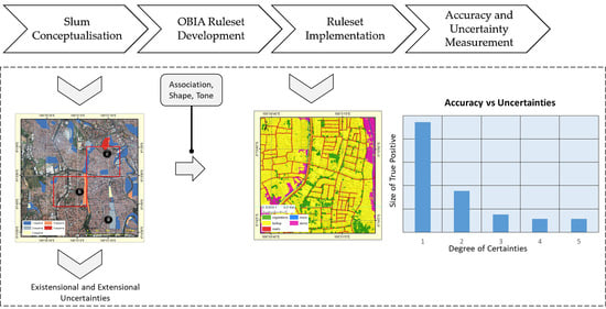
Our research methods are comprised of four main parts: (i) slums conceptualisation, (ii) OBIA ruleset development, (iii) ruleset implementation, (iv) accuracy and uncertainty measurement. Our methodology is shown in Figure 2, and the detailed process is described in the following paragraph.
In the first part, we related the definitions of slums by the local experts with image-based information by using several observable visual elements, e.g., tone, shape, size, texture and association [6,10]. We selected five local experts from different backgrounds, i.e., government, consultants and NGOs. As mentioned in [25], the selected experts needed to have a professional knowledge of slums. Therefore, we selected experts that have been involved in programs related to slums in Jakarta. From the government, we have interviewed two experts, one from the National Government (Ministry of Public Works), and one from the Local Government (Department of Spatial Planning, Jakarta). In addition, we interviewed two experts from consultancies that were involved in formulating the national policy of slums in Indonesia. Lastly, we interviewed one representative from an NGO, who participated in monitoring settlement targets for the Millennium Development Goals (MDG). Besides expert interviews, field observations were conducted in the areas experts delineated as slums. The characteristics of slums obtained during the interviews were used for developing the ruleset for the OBIA-based slum detection.
In the second part, we developed the OBIA-based ruleset for slum detection according to the definitions mentioned in the first step. In general, OBIA aiming to relate geographic features with image objects can be divided into two main parts, namely segmentation and classification [40]. In general, segmentation delineates regions (segments) of an image that share common attributes [41]. The result is a relatively homogeneous and significant grouping of pixels [42]. Meanwhile, the classification process assigns each segment to a particular class according to predefined characteristics, e.g., tone, shape, size, texture and association. For segmentation, we used multi-resolution segmentation (MRS) since this algorithm has been widely used in OBIA-based slum detection studies (e.g., [5,12]). However, the implementation of MRS is dependent on the Scale Parameter (SP) [43], controlling the heterogeneity of image objects [44]. The SP value is often selected in a trial-and-error process [45]. Therefore, we employed the Estimation Scale Parameter (ESP) tool [43] to determine the most appropriate SP.
In the third part, we implemented the ruleset in our study area. We selected Pleiades imagery granted from the European Space Agency (ESA) with standard-ortho bundles for the year of 2015, with a spatial resolution of 0.5-m for R-G-B-NIR bands. We managed to obtain an image with a cloud cover of less than 10%. We purposively selected two small test areas (sized km2)), without any cloud cover. For the first test area, we selected an area with a relatively similar agreement of slum boundaries among experts, while, in the second area, experts considerably disagreed about slum boundaries.
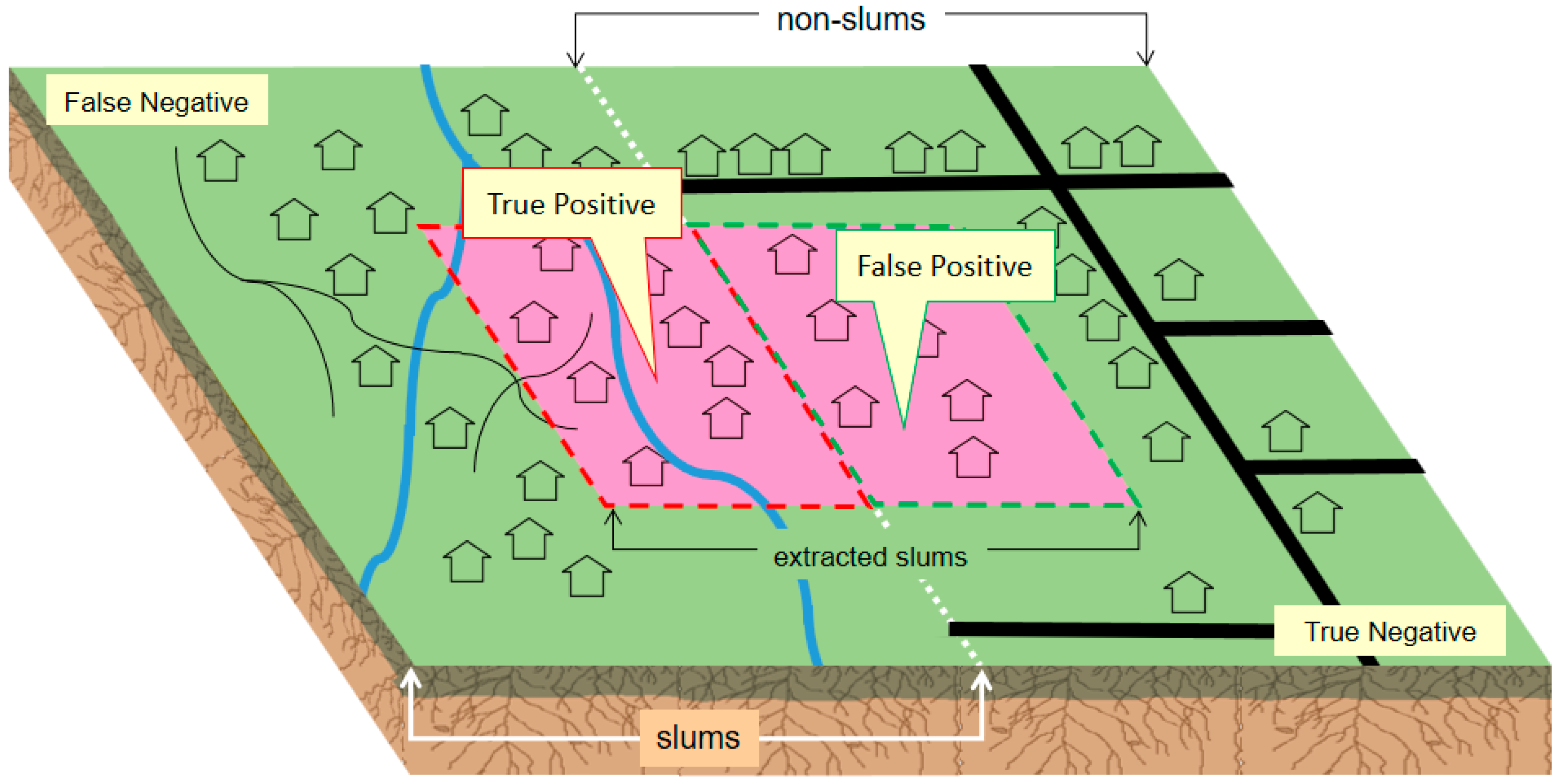
Lastly, in the fourth part, we measured the accuracy of the classification result. Manual delineation of slum boundaries (on top of the image) by local experts were used to produce the reference data, as demonstrated in [24,25]. Thus, we compared the extracted slums from the OBIA ruleset, with the reference data from the local experts. This comparison obtained four possible results (Figure 3), i.e., true positive (TP), false positive (FP), true negative (TN) and false negative (FN).
We used three indicators for measuring accuracy, i.e., precision, recall and accuracy. Precision or confidence describe the proportion of predictive-positive cases, which show a correct match with the reference data [46]. It can be measured by comparing TP with TP and FP (1). Meanwhile, recall or sensitivity indicates the proportion of real positive cases that were correctly predicted. It can be measured by comparing the number of TP, with TP and FN (2). Lastly, accuracy indicates the total correct positive and negative cases (i.e., TP and TN) to the total number of possible cases (i.e., TP, FP, FN, TN) (3) [46]. Therefore, precision, recall and accuracy were calculated as:
Regarding uncertainties, as pointed out in [25], the difficulties to draw exact boundaries where slums change into non-slums and vice versa leading to uncertainty, i.e., existential and extensional uncertainty [47]. First, existential uncertainty indicates the degree of confidence whether a slum exists in reality [25,47], and it may depend on experts’ experience or conceptual difference upon image interpretations [25]. Second, extensional uncertainty indicates the area delineated as a slum with limited certainty [25].
Furthermore, uncertainties also arose from different slum conceptualizations by local experts. While [25] aimed to study the deviations of slum boundaries observed from Very High Resolution (VHR) images, our research emphasises the impact of various degrees of slum boundaries’ agreements on the values of the accuracy assessment. To do so, we compared the classification result (OBIA slum map for each test area) obtained in the third part with the reference data showing various agreement levels. For instance, first, we compared the classification result with an area where the reference data showed the highest agreement (all five experts agreed that an area is a slum). Next, we measured the accuracy according to the indicators mentioned in (1) to (3). We repeated this procedure for each subset and every degree of agreement (ranging from 1 to 5 experts). This comparison allowed us to examine the impact of different agreements in the reference data on accuracy levels for mapping slums in Jakarta.
4. Results
4.1. Slums Conceptualisation
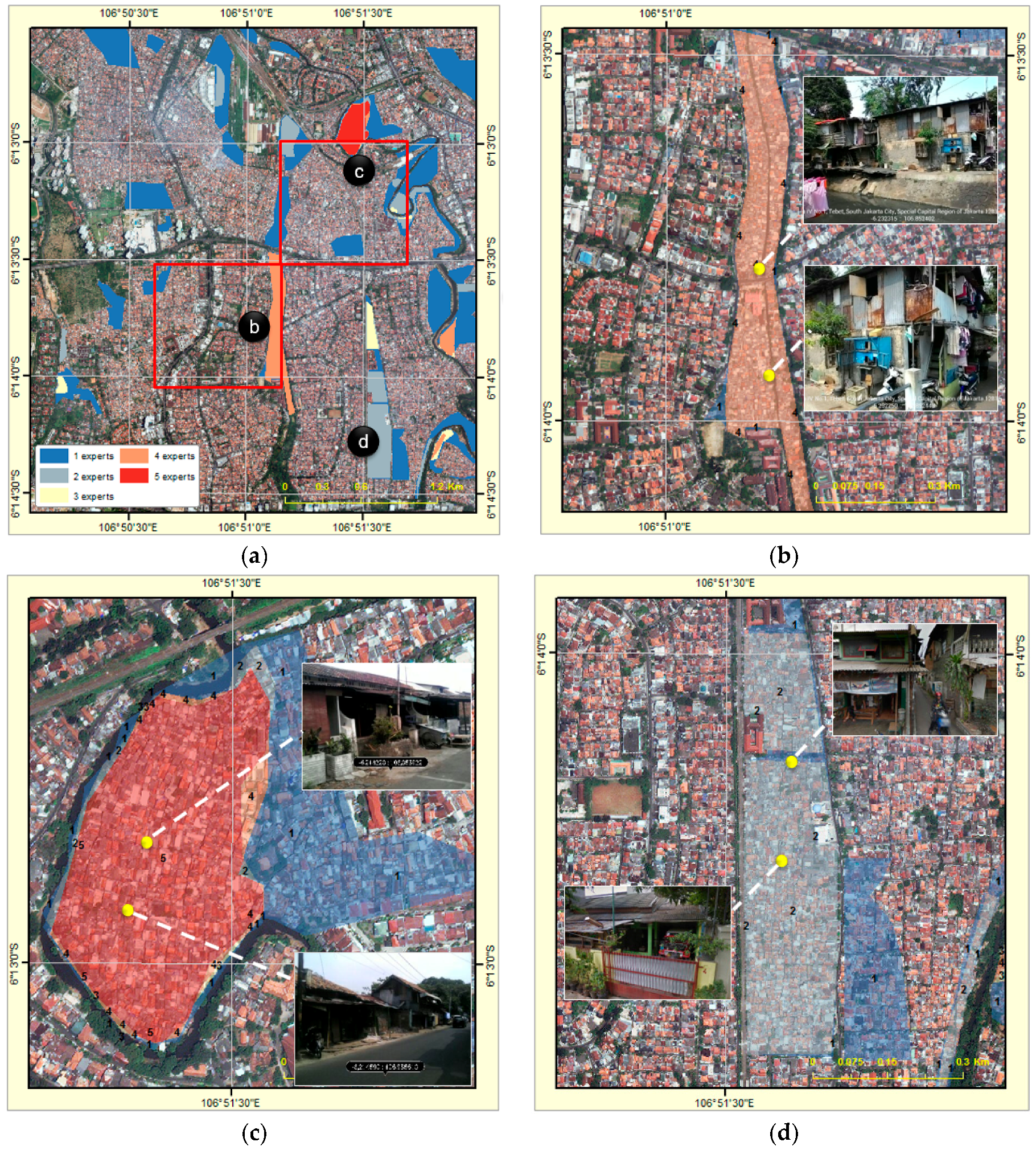
The result of the expert interviews shows the local diversity of slum characteristics (Table 1). The expert from the national institutions (i.e., Ministry of Public Works) defined slums according to the building size, which, in general, is smaller in size compared to non-slum buildings. In addition, slums are located commonly on the riverbank or near railroads, with irregular building orientations. The expert from the local government mentioned similar characteristics regarding the location on the riverbank and near railroads. With regards to the difficulties to distinguish slum and non-slum kampungs, the tenure status was often mentioned as a characteristic that could be used for distinguishing. Experts (NGO and two consultants) also came up with the slum characteristic of small building sizes. In addition, they also mentioned that slums have irregular building orientations, poor roof materials and are located on the riverbank and near railroads. The last expert (the second consultant), however, only mentioned building size and irregular building orientation as slums characteristics.
According to the visual image interpretations, local experts have different agreements on slum locations in our study area. In Figure 4a, we show the different agreements of slum extents (delineated by experts), where the red area and blue areas indicate the highest and lowest agreement respectively. To give a better understanding regarding slum characteristics on the ground, we conducted field observations. For the first sample (Figure 4b), we selected an area along the Tebet Timur Street, which was digitized by four of our experts. From field observations, this area is characterised by its proximity to the river and has irregular building orientations. We also found that buildings in this area are made up of poor materials (e.g., cardboard, plastics, corrugated iron, woven bamboo). In addition, we noticed different types of roof materials (i.e., ranging from tiles to corrugated irons). For the second example, we selected an area in Manggarai I street (Figure 4c), which shows diversity in terms of expert agreements on slums (ranging from one to five experts).
4.2. OBIA Ruleset Development
When developing the OBIA ruleset, we translated the characteristics of slums obtained from the local experts, into characteristics that can be recognised by a computer. The association may include tone, shape, size, texture and associations. Table 2 shows the five characteristics of slums that are used to develop the ruleset.
For the first characteristic, slums are commonly located on the riverbank or near the railroad. Thus, we employed a vector layer of rivers and railroad (Openstreet Map data) using proximity as a rule. For the second and third characteristics, we associate the size and shape of the building with the shape and size of the segment. Meanwhile, for the fourth characteristic, we associate the roof material of slum buildings with the tone/colour of the segment. The last characteristic is most interesting. Unlike the four previous characteristics, the last one is not directly observable from an image. Therefore, we used a proxy indicator to determine the tenure status. According to the interview with the expert from the Jakarta province, Jakarta is implementing a strict zoning regulation, which means it is illegal to construct within protected zones. Thus, we decided to use the zoning map to delineate the protected zones, where any construction is illegal and has no legal tenure status.
The idea of using a non-observable indicator has induced us to develop two scenarios when implementing our ruleset. First, we run our ruleset with four indicators (only observable; indicator number 1 to 4 in Table 2). Second, we include the non-observable indicator (number 5 in Table 2). We applied both scenarios for the two test areas.
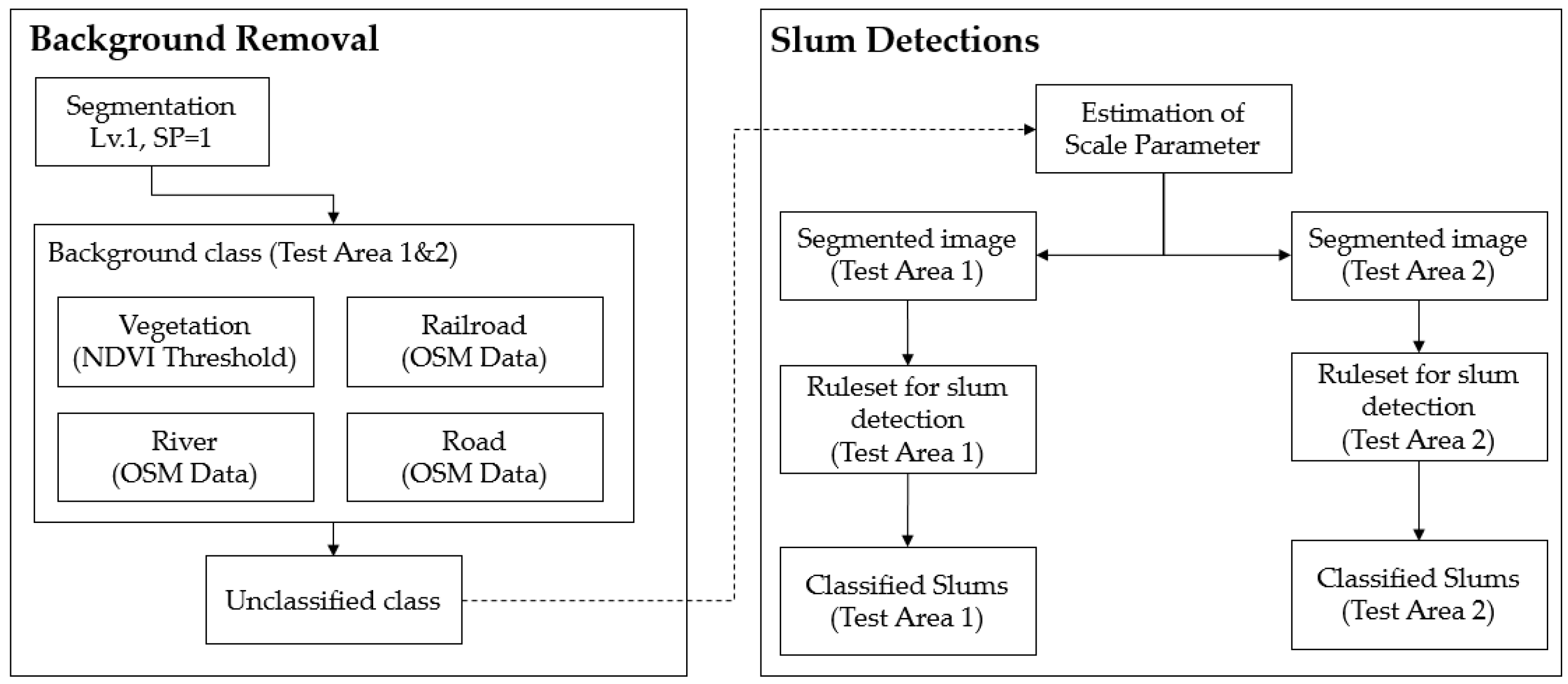
After we associate each slum characteristic with its consecutive image domain, we develop our ruleset in Trimble’s eCognition, Developer version 9 (Trimble Germany GmbH, Munich, Germany). Our ruleset can be divided into two steps (Figure 5)—first, background removal, and, second, slum detection. In the background removal step, we implement MRS with a low SP (SP = 1) to extract background classes, i.e., vegetation, railroads, roads, and the rivers. Next, we apply a coarse segmentation for the remaining unclassified segments, and here we implement our ruleset for slum detection.
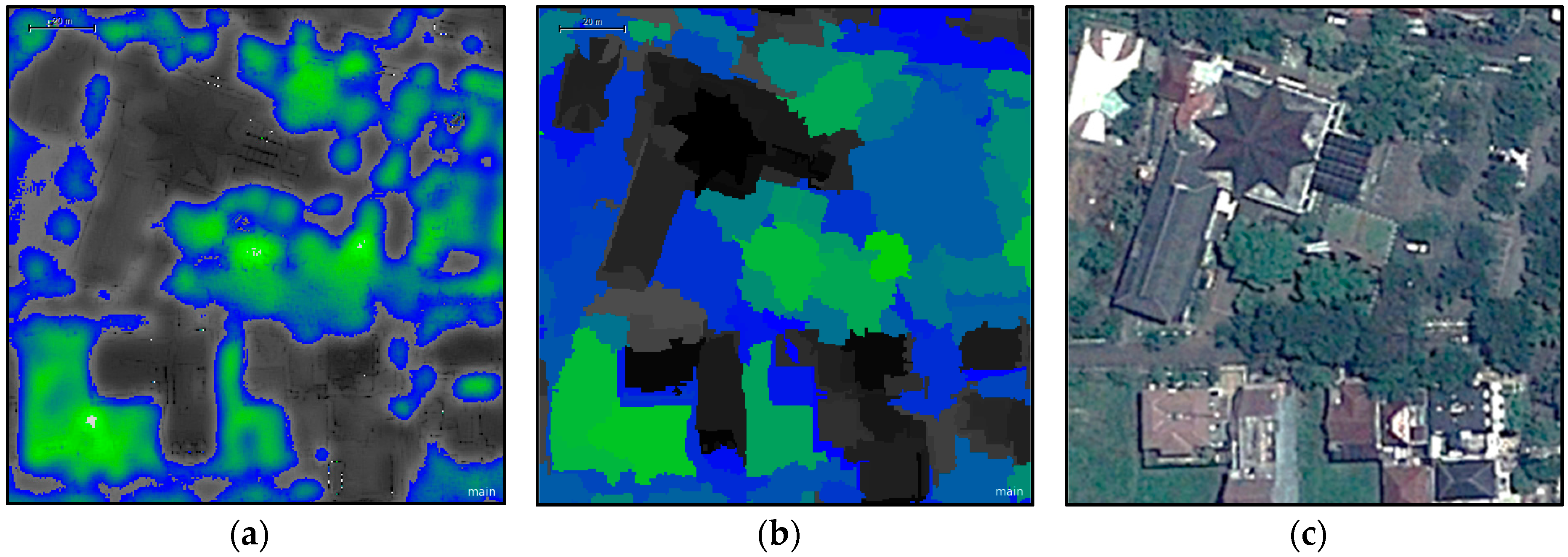
In the first step, we find that, among various possible associations (i.e., tone, shape, size, texture and associations), which can be used for classification, the Normalized Difference Vegetation Index (NDVI: proportion between near-infrared and red band) shows its ability to detect the vegetation well. Each object that has an average value of NDVI greater than zero is classified as vegetation. However, if we choose a coarse segmentation, vegetation is under-segmented (Figure 6). Hence, we are intentionally over-segmenting because we aim to obtain the shape and size of the vegetation class as close as possible to its real shape and size.
For the remaining background classes (i.e., road, railroad, river), we classify the segments using vector data. For this purpose, we also implemented a fine segmentation for these classes. After we classified all background classes, the remaining class (i.e., unclassified) has a certain probability to be classified as a slum. Here, we implement the second step.
In this second step, we re-segment the unclassified class, aiming at coarser segments. The ESP can produce three levels of segmentation, which can be associated with three levels of slums objects as mentioned in [5]. Since slum buildings are characterised by their small size (Table 2), it is difficult to extract every single building as an object. Therefore, we use the second level of SP obtained from ESP, which is 95.
After conducting the segmentation process, we implement our concept of slums to develop the ruleset for classifying each test area. The threshold values were obtained through a trial and error process, and we assigned these values into the class description in eCognition software (version, Manufacturer, City, US State abbrev., Country) (Table 3).
For the first rule, we use the border to the river and railroad and assign each object that has more than zero pixels touching the border of river/railroad as a slum. Regarding shape, we implement two rules, compactness and grey level co-occurrence matrix (GLCM) dissimilarity. Compactness indicates the variations among pixels under one object. The lower the compactness, the higher the variation of pixel values. Regarding GLCM dissimilarity, the higher the value, the less that the pixel values show similarity within one segment [48]. For the tone, since the roof materials of slum houses in our study area are predominated by tiles or corrugated iron, we find that the average of red/green shows a linear relationship with the roof colour. Here, we use the band arithmetic approach in eCognition by calculating the proportion of red and green band in each segment. The last rule is only applicable to the second scenario. To develop this rule, we first converted the zoning map of the study area from vector to raster. Then, we reclassified the value of each land use class into two labels, i.e., have tenure and no tenure. Next, this binary image is segmented using MRS (the zoning map was not used within the segmentation as not all scenarios were using the zoning map as ancillary data). We calculate the ‘tenure value’ of each segment and identify the threshold for slums. The more the segmented image overlapped with the ‘tenure segment’, the higher the chance that the segment is a slum.
We use “OR” function for association in our ruleset, which means that a slum may be located near the river, or near the railroad, or in the proximity of both of them. Meanwhile, for the rest of the indicators, we use the “AND” function, which means that the object must meet all threshold value to be classified as slums.
4.3. Ruleset Implementation
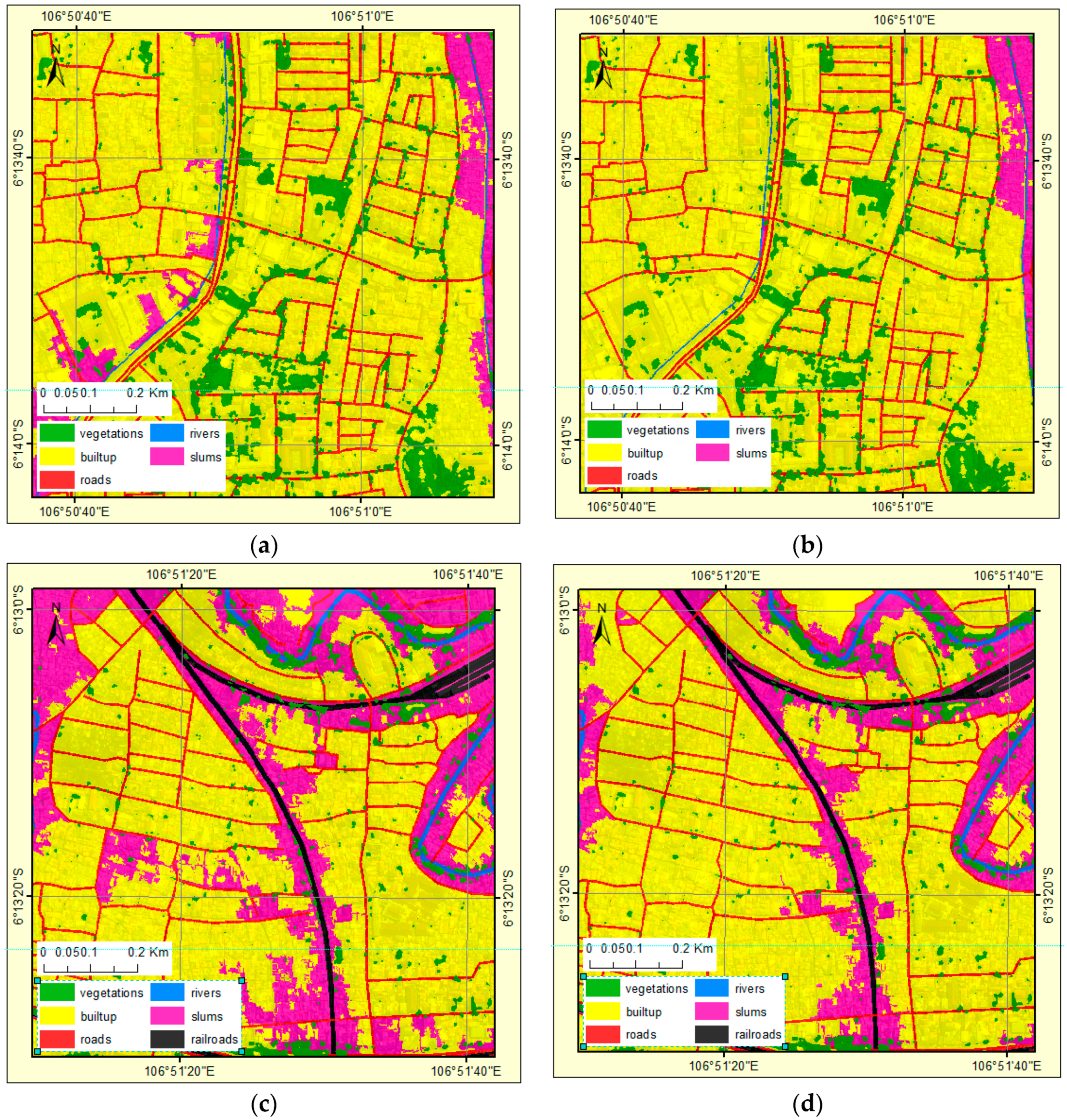
We implement our ruleset in the first test area (clear boundaries between slum and non-slum), and the second area (unclear boundaries). In addition, we implement our ruleset for two scenarios, first with using tenure status as an additional proxy, and second without tenure status. Hence, the four pairs of results are shown in Figure 7.
In Figure 7, we notice some similarities and differences in the classification results for the different scenarios. Figure 7a,b is an area where slum and not slum areas have clear boundaries. In Figure 7a, where the tenure indicator is not implemented, we find two slum zones, which are located in the western and eastern parts of this area. Meanwhile, in Figure 7b, implementing the tenure indicator, only the eastern part is classified as a slum. Furthermore, Figure 7c,d refers to the area where slum and not slum areas have unclear boundaries. The results show similarities of slum patches in the eastern part in Figure 7a,b while result Figure 7c,d show a more distinct pattern of slums. However, we also find similarities of slum patches for the second test area, particularly for slums that are located near the railroad or the river.
4.4. Accuracy and Uncertainty Measurements
For each classification results shown in Figure 7, we compared with the degree of agreements by experts, which ranges from five (highest agreement) to only one agreement (only selected by one expert (reference data). This results in twenty possible values for each accuracy indicator mentioned in Equations (1) to (3). Table 4 shows the size of true positive (TP), false positive (FP) and false negative (FN), measured in square meters.
The number of TP indicates the size of the area that is detected as slums by the OBIA classification as well as in the reference data. We find differences in the amount of TP between TA1 and TA2, also between EXP and ANC. Apparently, the difference between EXP and ANC in TA1 is lower than in TA2. Both areas and scenarios show similarities related to the number of agreements. As we reduce the required degree of agreements for the reference data (from 4 to 1 in TA1, and from 5 to 1 in TA2), the size of TP is increasing. However, we only find two degrees of agreement in TA1 (i.e., one and four experts). Meanwhile, we find various levels of agreements in TA2, which indicates that our experts have very different perceptions concerning slum boundaries in TA2.
FP indicates the size of the area, which is detected as slums by the OBIA classification but is not delineated as slums by the experts. Interestingly, the difference of FP between EXP and ANC in TA1 is substantially greater than in TA2. In TA1, the size of FP in EXP is thirteen times higher than ANC. Meanwhile, the difference of FP in TA2 for EXP is only one-and-a-half times greater than ANC. TA1 and TA2 show similarities related to the degree of agreements. As we reduce the degree, we get a decreasing number of FP.
Lastly, the FN indicates the size of the area that is detected as a slum by the experts but not detected as a slum by the OBIA classification. We notice a similar pattern of FN between EXP and ANC in TA1 and TA2. As we decrease the number of required agreements, we have an increasing number of FN. However, the increasing of FN in TA1 (for EXP and ANC) is more gradual than in TA2. In TA2, we find a significant increase of FN when we reduce the agreement from 2 to 1. This points to very diverse perceptions by experts on slum boundaries in TA2. Therefore, it results in a substantial size of slum patches with only one agreement—Figure 4a in the red box labelled c. Using the value of TP, FP and FN, we calculate precision, recall and accuracy shown in Table 5.
Table 5 shows that the usage of tenure data in the first area results in a high precision. As shown in Equation (1), precision is measured by comparing TP with TP and FP. Hence, high precision results from a low FP, which indicates that our OBIA ruleset is only producing a small number of slums that are not delineated as slums by our experts.
In TA2, we notice substantial differences compared to TA1. Implementing the tenure status in TA2 results in the lowest precision compared to other combinations (i.e., TA1_EXP, TA1_ANC and TA2_EXP). This is due to the high number of FP, which are areas not delineated as a slum by experts but classified as a slum. Interestingly, in Figure 4a, the red box labelled c, no expert selecting the area adjacent to the railroad as slums. Figure 7c,d indicates that our ruleset is detecting areas adjacent to the railroad as slums since we used this in our ruleset (Table 2). Although TA1 and TA2 show significant differences of precision values, similarities exist across different degrees of slum agreement, reducing the required degree of agreements results in a higher precision value. These higher values result from lower FP, caused by an increase in the size of slum extents in the reference data.
Recall, as mentioned in Equation (2), is measured by comparing TP with TP and FN. Hence, the high values of recall result from low FN, and this indicates that only a small number of slums in the reference data is not detected as a slum by the OBIA ruleset. In general, 2015_TA2_ANC has the lowest recall value compared to others (Table 5). This indicates that, in 2015_TA2_ANC, many slums from the reference data are not detected by the OBIA ruleset. As shown in Figure 4a in the red box labelled c, experts have different perceptions of slum boundaries. Thus, selecting only areas with a high agreement in TA2 will result in high FN. Interestingly, if we compare recall values among different agreements in the reference data, only TA2_ANC shows a different pattern. The highest value is obtained for three agreements; however, differences across recall values are small. This indicates that settlements without tenure status have a high probability to be identified as a slum by the experts.
Regarding accuracy, we can point to the difference between TA1 and TA2. In TA1, the highest accuracy is achieved by the largest number of agreements. In TA2, slightly higher accuracy values are obtained by lower agreements. This pattern can be seen in both EXP and ANC scenarios. In general, our ruleset gains a higher accuracy when applied in TA1, where the slum boundaries are more clear. By comparing different locations, scenarios and indicators, we can examine the impact of the ruleset’s performance as we decreased the degree of agreement (from highest to lowest agreement) (Table 6).
Surprisingly, we notice that no data set gains more accuracy as we reduce the degree of agreement from the highest to the lowest. In Table 5, the maximum accuracy of every possible combination is never obtained by the lowest agreement. For a gain, we can notice that only TA2_ANC shows an increased gain as we decreased the level of agreement. Regarding precision, TA2 shows a significant increase of precision as we reduce the level of agreement.
5. Discussion
Image interpretations by experts are commonly used to measure the accuracy of OBIA classification results [25,49]. In this study, we employed reference data generated by manual delineation of local experts from varied backgrounds. From the results (Figure 4), we noticed different agreements regarding the extent of slums. Nonetheless, these differences cannot be qualified as inaccuracies, and every image interpretation is equally valid [24]. It is likely that the different interpretations are rather caused by the uncertainties existing in a particular area [24]. Comparing the slum delineations in our two test areas (Figure 4a, the red box labelled b and c), we can notice how these uncertainties caused variations on slum agreements among experts. In the first test area, agreements on slum locations and boundaries varied less compared to the second test area. During ground observations, we noticed clear boundaries of slums in the first test area (eastern part), and formal housing and commercial area (the western part). On the contrary, the second area is dominated by kampungs. As mentioned in Section 2, kampungs may consist of formal housing kampungs having also high built-up densities or slum kampungs commonly having very high built-up densities. These vague boundaries between slum and non-slum kampungs make it difficult to determine where exactly a slum changes into a non-slum [25].
Comparing OBIA classification with manual delineations can result in three scenarios (besides True Negative). First, slum delineations (experts) are outside the OBIA (slum) result, i.e., False Negative (FN). Second, OBIA results are outside slum delineations, i.e., False Positive (FP). Third, slum delineations are matching the OBIA result, i.e., True Positive (TP). In Table 4, we have shown how FN, FP and TP change across different level of agreements. In general, a higher level of agreement will lead to more certainty about the delineated slums. Regarding the first> scenario, TA1 and TA2 show a similar pattern, as we reduce the degree of certainty, the higher the FN results. For the second scenario, the lower the degree of certainty, the lower the FP. Meanwhile, for the third scenario, the highest TP is obtained with the lowest certainty. Thus, the more we try to match manual delineations and OBIA classification results, the higher the uncertainty will be.
Although we employed an ontology-based slum’ characterization starting from expert domain knowledge, this is solely done in the image classification step. Ontologies are commonly used in the classification part [15]; however, the potential use of ontologies in other phases requires further exploration. As mentioned by [15], the processing time needed is growing exponentially when more concepts are included into the ontology.
Regarding experts’ experience, we argue that our experts have a reasonable expertise and have a strong understanding of slums in Jakarta. Similar to [25], the level of experience is not a significant factor related to delineations’ accuracy. Meanwhile, regarding the conceptual differences, we noticed a different characterization of slums among expert (Table 1), which contributed to different delineations. However, it may not be the only cause. Previous research [50] indicated that the performance of experts in digitizing in an image is affected by internal and external factors. Internal factors include demographics, experience and skills, personality, memory span, motivation and comparative anxiety. The external factors may include quality of screen/images, amount of distraction, tiredness, and time of day. However, we do not further examine how this internal factor might impact the quality of slum identifications by our experts. However, we argue that some external factor affected the quality of slum identifications—for instance, tiredness and time of day. Our survey was taken in different sessions, i.e., during office hours, and after office hours. It is likely that interviews conducted after office hours affected the quality of image interpretation due to tiredness. All of these factors introduce uncertainties for the generation of reference data, which are commonly not made explicit. However, when aiming at remote sensing based slum mapping, it will be very important to make these uncertainties explicit and clarify how they relate to mapping accuracies. Making these uncertainties explicit is important for bridging the communication gap [50] between technical experts and planners. This will allow for better understanding the scope and limitations of OBIA based slum mapping in support of planning and decision making on monitoring the implementation of slum upgrading policies.
6. Conclusions
Our study aimed to analyse the uncertainties in measuring the accuracy of OBIA-based slum detection in Jakarta, Indonesia. Comparing the results of manual delineations of slum areas by experts with OBIA classification results, there are, in general, four possible outcomes, i.e., True Positives (TP), False Positives (FP), False Negatives (FN) and True Negatives (TN). The values of TP, FP, FN and TN, and the accuracy indices changed when the degree of expert agreements changed in the reference data. These different degrees of agreements demonstrated that there are uncertainties on the location and boundaries of slums, referred to as existential and extensional uncertainties, respectively. This outcome stresses the dilemma faced by slum mapping campaigns. Furthermore, our study demonstrated the role of a non-observable indicator (land tenure), in order to assist slum detection, particularly when uncertainties exist. However, the recall of our classification result decreased by introducing this additional indicator, while the classification accuracies increased. The inherent uncertainties in reference data (even within a city, there is limited agreement on what defines a slum and where are the boundaries between slum and non-slum areas) emphasise the need to include uncertainty analysis in slum mapping approaches besides assessing classification accuracies. We also need to build slum ontologies that integrate local knowledge when aiming for a city or nationwide slum mapping and monitoring campaigns employing VHR imagery. However, the transferability of slum mapping indicators that are very context specific is limited, i.e., indicators might work well in one area but may lead to an increase in uncertainties and/or lower accuracies in other areas. Based on the findings of our research, we conclude that slum mapping studies need to better address uncertainties embedded in reference data for developing a transferable and robust set of indicators. Considering the entire uncertainties when producing reference data, it is critical to explicitly clarify their influence on classification results. This will be a first stepping-stone towards generating a knowledge base, which allows for providing base information but also has the potential to bridge the communication gap between remote sensing experts and domain experts (i.e., planners—policy makers). Furthermore, such uncertainty analysis will lead to better understanding where remote sensing can assist in planning and decision making in the context of slum upgrading projects and policies.
Acknowledgments
We obtained Pleiades imagery that was used in this research from the European Space Agency (ESA).
Author Contributions
Jati Pratomo designed the research framework and wrote the draft of the manuscript. Monika Kuffer revised and edited the manuscript and gave advice on the research design. Javier Martinez gave advice on paper writing and research design. Divyani Kohli gave advice on ruleset development and uncertainty measurement and supported the review of the manuscript.
Conflicts of Interest
The authors declare no conflict of interest.
References
- Open Working Group SDG. Sustainable Development Goals Open Working Group Proposal for Sustainable Development Goals; Division for Sustainable Development, United Nations: New York, NY, USA, 2014. [Google Scholar]
- United Nations. The Millennium Development Goals Report; United Nations: New York, NY, USA, 2014. [Google Scholar]
- UN Habitat. Slums Almanac 2015–16. Tracking Improvement in the Lives of Slum Dwellers; UN Habitat: Nairobi, Kenya, 2016. [Google Scholar]
- Shoko, M.; Smit, J. Use of Agent Based Modelling in the Dynamics of Slum Growth. S. Afr. J. Geomat. 2013, 2, 54–67. [Google Scholar]
- Kohli, D.; Kerle, N.; Sliuzas, R. Local ontologies for object-based slum identification and classification. In Proceedings of the 4th International Conference on Geographic Object-Based Image Analysis Conference (GEOBIA), Rio de Janeiro, Brazil, 7–9 May 2012; pp. 201–205. [Google Scholar]
- Hofmann, P.; Strobl, J.; Blaschke, T.; Kux, H. Detecting informal settlements from Quickbird data in Rio de Janeiro using an object based approach. In Object-Based Image Analysis; Lecture Notes in Geoinformation and Cartography; Blaschke, T., Lang, S., Hay, G.J., Eds.; Springer: Berlin/Heidelberg, Germany, 2008; pp. 531–553. [Google Scholar]
- Kohli, D.; Warwadekar, P.; Kerle, N.; Sliuzas, R.; Stein, A. Transferability of object-oriented image analysis methods for slum identification. Remote Sens. 2013, 5, 4209–4228. [Google Scholar] [CrossRef]
- Kuffer, M.; Pfeffer, K.; Sliuzas, R.; Baud, I.; van Maarseveen, M. Capturing the Diversity of Deprived Areas with Image-Based Features: The Case of Mumbai. Remote Sens. 2017, 9, 384. [Google Scholar] [CrossRef]
- Ebert, A.; Kerle, N.; Stein, A. Urban social vulnerability assessment with physical proxies and spatial metrics derived from air- and spaceborne imagery and GIS data. Nat. Hazards 2009, 48, 275–294. [Google Scholar] [CrossRef]
- Kohli, D.; Sliuzas, R.; Kerle, N.; Stein, A. An ontology of slums for image-based classification. Comput. Environ. Urban Syst. 2012, 36, 154–163. [Google Scholar] [CrossRef]
- Hofmann, P. Defining Robustness Measures for OBIA Framework: A Case Study for Detecting Informal Settlements. In Global Urban Monitoring and Assessment through Earth Observation; Weng, Q., Ed.; CRC Press: Boca Raton, FL, USA, 2014; pp. 303–324. [Google Scholar]
- Kuffer, M.; Barros, J.; Sliuzas, R. The development of a morphological unplanned settlement index using very-high-resolution (VHR) imagery. Comput. Environ. Urban Syst. 2014, 48, 138–152. [Google Scholar] [CrossRef]
- Gilbert, A. The return of the slum: Does language matter? Int. J. Urban Reg. Res. 2007, 31, 697–713. [Google Scholar] [CrossRef]
- Forestier, G.; Puissant, A.; Wemmert, C.; Gançarski, P. Knowledge-based region labeling for remote sensing image interpretation. Comput. Environ. Urban Syst. 2012, 36, 470–480. [Google Scholar] [CrossRef]
- Andrés, S.; Arvor, D.; Mougenot, I.; Libourel, T.; Durieux, L. Ontology-based classification of remote sensing images using spectral rules. Comput. Geosci. 2017, 102, 158–166. [Google Scholar] [CrossRef]
- Anders, N.S.; Seijmonsbergen, A.C.; Bouten, W. Rule Set Transferability for Object-Based Feature Extraction: An Example for Cirque Mapping. Photogramm. Eng. Remote Sens. 2015, 81, 507–514. [Google Scholar] [CrossRef]
- Tiede, D.; Lang, S.; Hölbling, D.; Füreder, P. Transferability of OBIA rulesets for IDP camp analysis in darfur. ISPRS 2010, XXXVIII-4/C7, 1682–1777. [Google Scholar]
- Drǎguţ, L.; Blaschke, T. Automated classification of landform elements using object-based image analysis. Geomorphology 2006, 81, 330–344. [Google Scholar] [CrossRef]
- Hofmann, P.; Blaschke, T.; Strobl, J. Quantifying the robustness of fuzzy rule sets in object-based image analysis. Int. J. Remote Sens. 2011, 32, 7359–7381. [Google Scholar] [CrossRef]
- Hofmann, P. Detecting Informal Settlements From Ikonos Image Data Using Methods of Object Oriented Image Analysis—An Example From Cape Town (South Africa). In Proceedings of the Remote Sensing of Urban Areas/Fernerkundung in Urbanen Räumen, Regensburg, Germany, 22–23 June 2001; pp. 107–118. [Google Scholar]
- Albrecht, F. Assessing the spatial accuracy of object-based image classifications. In Proceedings of the Geospatial Crossroad (GI_Forum ’08), Salzburg, Austria, 1–4 July 2008; pp. 11–20. [Google Scholar]
- Zhang, J.; Goodchild, M.F. Uncertainty in Geographical Information; Taylor & Francis: London, UK, 2002; p. 266. [Google Scholar]
- Schiewe, J.; Gähler, M. Modelling uncertainty in high resolution remotely sensed scenes using a fuzzy logic approach. In Object-Based Image Analysis; Lecture Notes in Geoinformation and Cartography; Blaschke, T., Lang, S., Hay, G.J., Eds.; Springer: Berlin, Germany, 2008; pp. 755–768. [Google Scholar]
- Albrecht, F. Uncertainty in Image Interpretation as Reference for Accuracy Assessment in Object-based Image Analysis. In Proceedings of the Accuracy 2010 Symposium, Leicester, UK, 20–23 July 2010; pp. 13–16. [Google Scholar]
- Kohli, D.; Stein, A.; Sliuzas, R. Uncertainty analysis for image interpretations of urban slums. Comput. Environ. Urban Syst. 2016, 60, 37–49. [Google Scholar] [CrossRef]
- Demographia World Urban Areas; Belleville. Available online: http://www.demographia.com/db-worldua.pdf (accessed on 13 November 2017).
- Centre on Housing Rights and Evictions. Women, Slums and Urbanization: Examining the Causes and Consequences; Centre on Housing Rights and Evictions (COHRE): Geneva, Switzerland, 2008; pp. 1–134. [Google Scholar]
- New Cities Foundation. Jakarta to host 2015 New Cities Summit: “ This is Indonesia’ s Moment”. In New Cities Foundation; New Cities Foundation: Jakarta, Indonesia, 2015; pp. 1–3. [Google Scholar]
- UN Habitat. Indonesia Prepares National Report for Habitat III. Available online: http://unhabitat.org/indonesia-prepares-national-report-for-habitat-iii/ (accessed on 24 August 2017).
- Ministry of Public Works and Public Housing. Draft of Technical Documents on Monitoring and Evaluation of Spatial Planning; Ministry of Public Works and Public Housing: Jakarta, Indonesia, 2015. [Google Scholar]
- Pratomo, J. Transferability of the Generic and Local Ontology of Slum in Multi-Temporal Imagery, Case Study: Jakarta. Master’s Thesis, University of Twente, Enschede, The Netherlands, 2016. [Google Scholar]
- Redefining the Spatial Form of Urban Village in Mega Kuningan Jakarta as A New Urban Integrator: A Study of Socio-Economic Aspect in the Forming of Urban Spatial Configuration. Master’s Thesis, The University of Hong Kong, Hong Kong, China, 2009.
- Rukmana, D. Planning the Megacity: Jakarta in the Twentieth Century. J. Am. Plan. Assoc. 2008, 74, 263–264. [Google Scholar] [CrossRef]
- Sihombing, A. Drawing Kampung through Cognitive Maps Case Study: Jakarta. APCBEE Procedia 2014, 9, 347–353. [Google Scholar] [CrossRef]
- Sihombing, A. Living in the Kampungs: A Firsthand Account of Experiences in Jakarta’s Kampungs. Forum J. Postgrad. Stud. Archit. Plan. Landsc. 2007, 7, 15–22. [Google Scholar]
- Zhu, J.; Bunnell, T.; Yeo, V. Symmetric Development of Informal Settlements and Gated Communities: Capacity of the State—The Case of Jakarta, Indonesia; Asia Research Institute, National University of Singapore: Singapore, 2010. [Google Scholar]
- Indonesian Central Board of Statistics. Indikator Rumah Tangga Kumuh [Slum Household Indicator]. Available online: http://sirusa.bps.go.id/index.php?r=indikator/view&id=453 (accessed on 4 October 2016).
- Ministry of Public Works and Public Housing. Panduan Penyusunan SPPIP dan RPKPP [Guideline for Urban Settlement and Infrastructure Development]; Ministry of Public Works and Public Housing: Jakarta, Indonesia, 2014. [Google Scholar]
- UN Habitat. The Challange of Slum, Global Report on Human Settlements 2003; Earthscan Publication Ltd.: Nairobi, Kenya, 2003. [Google Scholar]
- Arvor, D.; Durieux, L.; Andrés, S.; Laporte, M.A. Advances in Geographic Object-Based Image Analysis with ontologies: A review of main contributions and limitations from a remote sensing perspective. ISPRS J. Photogramm. Remote Sens. 2013, 82, 125–137. [Google Scholar] [CrossRef]
- Liu, Y.; Guo, Q.; Kelly, M. A framework of region-based spatial relations for non-overlapping features and its application in object based image analysis. ISPRS J. Photogramm. Remote Sens. 2008, 63, 461–475. [Google Scholar] [CrossRef]
- Blaschke, T. Object based image analysis for remote sensing. ISPRS J. Photogramm. Remote Sens. 2010, 65, 2–16. [Google Scholar] [CrossRef]
- Drǎguţ, L.; Tiede, D.; Levick, S.R. ESP: A tool to estimate scale parameter for multiresolution image segmentation of remotely sensed data. Int. J. Geogr. Inf. Sci. 2010, 24, 859–871. [Google Scholar] [CrossRef]
- Baatz, M.; Schäpe, A. Multiresolution Segmentation: An optimization approach for high quality multi-scale image segmentation. In Angewandte Geographische Informationsverarbeitung XII; Strobl, J., Blaschke, T., Griesebner, G., Eds.; Wichmann: Heidelberg, Germany, 2000; pp. 12–23. [Google Scholar]
- Whiteside, T.G.; Boggs, G.S.; Maier, S.W. Comparing object-based and pixel-based classifications for mapping savannas. Int. J. Appl. Earth Obs. Geoinf. 2011, 13, 884–893. [Google Scholar] [CrossRef]
- Powers, D.M.W. Evaluation: From Precision, Recall and F-Factor to ROC, Informedness, Markedness & Correlation. J. Mach. Learn. Technol. 2011, 2, 37–63. [Google Scholar]
- Molenaar, M. Three Conceptual Uncertainty Levels for Spatial Objects. In Proceedings of the International Archieves of Photogrammetry and Remote Sensing, Amsterdam, The Netherlands, 16–22 July 2000; ISPRS: Amsterdam, The Netherlands, 2000; pp. 670–677. [Google Scholar]
- Trimble Germany GmbH. User Guide—eCognition® Developer, 9.1.1 ed.; Trimble: Munich, Germany, 2015; p. 256. [Google Scholar]
- Van Coillie, F.; Gardin, S.; Anseel, F.; Ducyk, W.; Verbeke, L.P.C.; de Wulf, R.R. Variability of Operator Performance in Remote-sensing Image Interpretation: The Importance of Human and External Factors. Int. J. Remote Sens. 2014, 35, 754–778. [Google Scholar] [CrossRef]
- Silva, C.; Bertolini, L.; te Brömmelstroet, M.; Milakis, D.; Papa, E. Accessibility instruments in planning practice: Bridging the implementation gap. Transp. Policy 2017, 53, 135–145. [Google Scholar] [CrossRef]
Figure 1.
Map of the study area in Jakarta Province (Indonesia) (a), surrounded by Banten Province and West Java Province (the metropolitan area includes some parts of these provinces), area boundary source: Openstreet Map (2015) (OpenStreetMap Foundation, Sutton Coldfield, UK); (b) selected subset located in Tebet district, Jakarta. Image source: Google Earth (2015) (Mountain View, CA, USA).
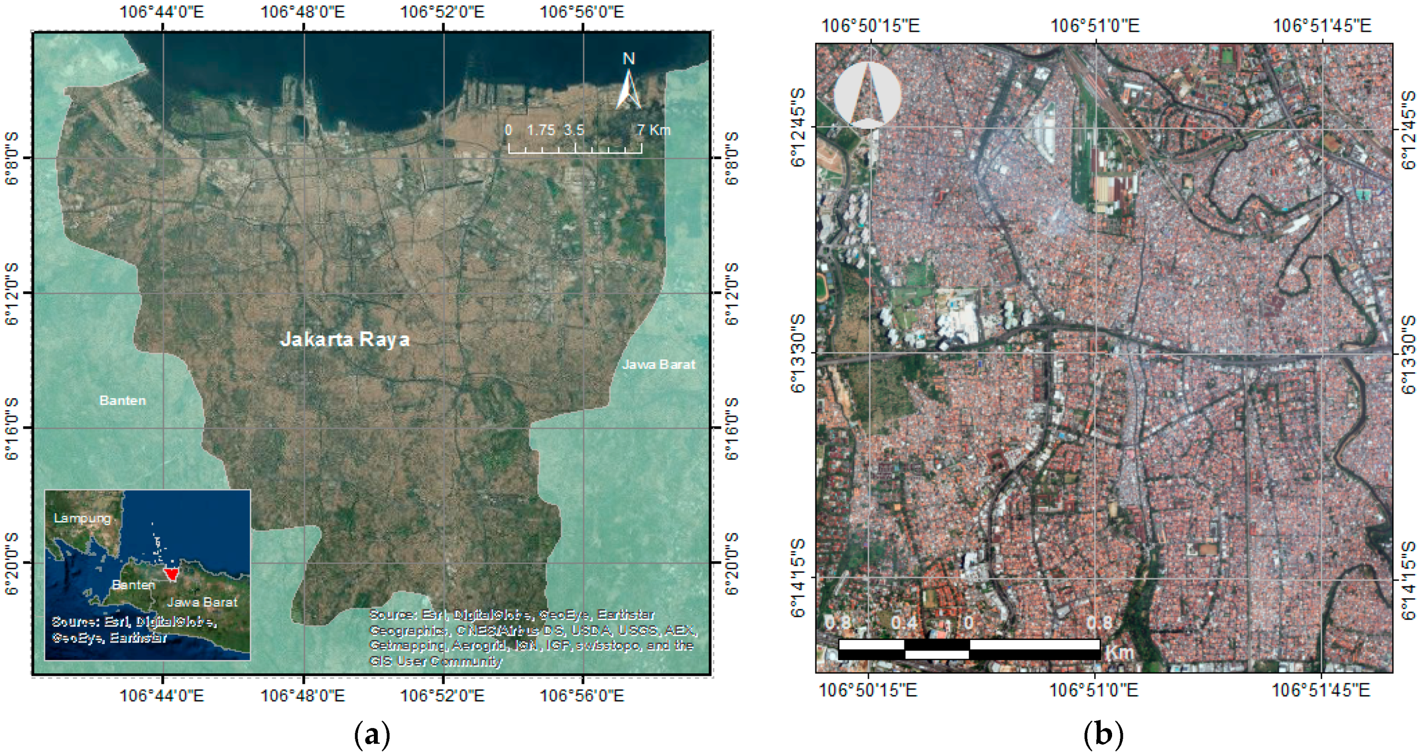
Figure 2.
Research methodology comprised of four main parts and their following activities.

Figure 3.
Four possible results from combining classification result with the reference data produced by the experts.
Figure 3.
Four possible results from combining classification result with the reference data produced by the experts.

Figure 4.
Slums extracted from manual delineation by different experts. (a) shows the different agreements of slum extents, where the red colour indicates areas with the highest agreement and the blue colour indicates the lowest; (b) shows the ground conditions of slums where four experts agreed; (c) shows the ground conditions of slums, which were indicated as a slum by all experts; (d) shows the ground conditions of a slum that was selected by one and two experts. The red boxes in (a) indicate our test areas.

Figure 5.
Object Based Image Analysis (OBIA) ruleset flowchart, which starts with background removal, followed by slum detection.
Figure 5.
Object Based Image Analysis (OBIA) ruleset flowchart, which starts with background removal, followed by slum detection.

Figure 6.
Impact of segmentation scale on vegetation classification. (a) shows segments with an Normalized Difference Vegetation Index (NDVI) of greater than zero obtained from fine segmentation and (b) from coarse segmentation, and (c) image before the segmentation process.
Figure 6.
Impact of segmentation scale on vegetation classification. (a) shows segments with an Normalized Difference Vegetation Index (NDVI) of greater than zero obtained from fine segmentation and (b) from coarse segmentation, and (c) image before the segmentation process.

Figure 7.
Mapped slums in the first test area (a,b). (a) indicates slums without the tenure indicator (only consider explicit indicators); (b) indicates slum employing the tenure indicator. Meanwhile, (c,d) indicates slums in the second area, by including and excluding the tenure indicator, respectively.

Table 1.
Different characteristics and definitions of slums among local experts. (1) is from the central government; (2) is from the local government; (3) is from Non-Government Organization (NGO), and (4) and (5) are housing policies consultants.
Table 1.
Different characteristics and definitions of slums among local experts. (1) is from the central government; (2) is from the local government; (3) is from Non-Government Organization (NGO), and (4) and (5) are housing policies consultants.
| Characteristics | Local Expert | |||||
|---|---|---|---|---|---|---|
| (1) | (2) | (3) | (4) | (5) | ||
| 1 | Located on/close the river bank/railroad | √ | √ | √ | √ | |
| 2 | Small building size | √ | √ | √ | √ | |
| 3 | Irregular building orientation | √ | √ | √ | √ | |
| 4 | Poor roof material | √ | √ | √ | ||
| 5 | Built on illegal land | √ | ||||
Table 2.
Translation of the real world characteristics into image domain characteristics in the context of the Generic and the Local Ontology of Slums.
Table 2.
Translation of the real world characteristics into image domain characteristics in the context of the Generic and the Local Ontology of Slums.
| Real World Domain | Image Domain | |
|---|---|---|
| 1 | Located on the riverbank/near railroad | Association: Distance to River/Railroad |
| 2 | Small building size | Size: Small |
| 3 | Irregular building orientation | Shape: compactness |
| 4 | Poor Roof material | Tone: Asbestos, corrugated iron |
| 5 | Built in the illegal land | Ancillary data: Land Use Plan |
Table 3.
Threshold value for each rule.
| Rule | Threshold Value |
|---|---|
| Association: Distance to River/Railroad | 1. Border to river > 0 pixels 2. Border to railroad 0 > pixels |
| Shape: compactness | 1. Compactness ≤ 5 2. Grey-Level Co-occurrence Matrix (GLCM) Dissimilarity ≥ 0.0005 |
| Tone: tile—corrugated iron, asbestos | Mean red/green 1 ≤ tone ≤ 1.075 |
| Ancillary data: Land Use Plan (second scenario) | Mean Layer Tenure > 0.25 |
Table 4.
The size (in m2) of true positive, false positive and false negative obtained by comparing classification results with the level of agreement. 2015_TA1_EXP indicates the year of the image, TA1 gives the location of the first test area (TA). EXP indicates that we only used explicit/observable indicators, while ANC means that we include an ancillary (not observable in images) indicator.
| Dataset | True Positive | |||||
| 5 | 4 | 3 | 2 | 1 | ||
| 2015_TA1_EXP | - | 41,321 | - | - | 41,802 |  |
| 2015_TA1_ANC | - | 36,209 | - | - | 36,690 |  |
| 2015_TA2_EXP | 11,397 | 11,938 | 15,155 | 35,486 | 94,480 |  |
| 2015_TA2_ANC | 3905 | 4445 | 7662 | 19,328 | 57,517 |  |
| Dataset | False Positive | |||||
| 5 | 4 | 3 | 2 | 1 | ||
| 2015_TA1_EXP | - | 31,763 | - | - | 31,281 |  |
| 2015_TA1_ANC | - | 2502 | - | - | 2021 |  |
| 2015_TA2_EXP | 228,686 | 228,146 | 224,929 | 204,598 | 145,604 |  |
| 2015_TA2_ANC | 156,702 | 156,162 | 152,945 | 141,279 | 103,090 |  |
| Dataset | False Negative | |||||
| 5 | 4 | 3 | 2 | 1 | ||
| 2015_TA1_EXP | - | 56,656 | - | - | 73,609 |  |
| 2015_TA1_ANC | - | 61,768 | - | - | 78,721 |  |
| 2015_TA2_EXP | 7217 | 9701 | 10,280 | 28,408 | 96,939 |  |
| 2015_TA2_ANC | 14,710 | 14,156 | 14,727 | 42,044 | 133,902 |  |
 Highest Value Highest Value  Other Values Other Values | ||||||
Table 5.
Accuracy values (i.e., precision, recall and accuracy) of classification results for the first and second area, two scenarios and different degrees of agreement.
Table 5.
Accuracy values (i.e., precision, recall and accuracy) of classification results for the first and second area, two scenarios and different degrees of agreement.
| Dataset | Precision | |||||
| 5 | 4 | 3 | 2 | 1 | ||
| 2015_TA1_EXP | - | 56.54% | - | - | 57.20% |  |
| 2015_TA1_ANC | - | 93.54% | - | - | 94.78% |  |
| 2015_TA2_EXP | 4.75% | 4.97% | 6.31% | 14.78% | 39.35% |  |
| 2015_TA2_ANC | 2.43% | 2.77% | 4.77% | 12.03% | 35.81% |  |
| Dataset | Recall | |||||
| 5 | 4 | 3 | 2 | 1 | ||
| 2015_TA1_EXP | - | 42.17% | - | - | 36.22% |  |
| 2015_TA1_ANC | - | 36.96% | - | - | 31.79% |  |
| 2015_TA2_EXP | 61.23% | 55.17% | 59.58% | 55.54% | 49.36% |  |
| 2015_TA2_ANC | 20.98% | 23.90% | 34.22% | 31.49% | 30.05% |  |
| Dataset | Accuracy | |||||
| 5 | 4 | 3 | 2 | 1 | ||
| 2015_TA1_EXP | - | 91.16% | - | - | 89.51% |  |
| 2015_TA1_ANC | - | 93.57% | - | - | 91.93% |  |
| 2015_TA2_EXP | 76.41% | 76.22% | 76.48% | 76.70% | 75.75% |  |
| 2015_TA2_ANC | 82.86% | 82.97% | 83.23% | 81.67% | 76.30% |  |
 Highest Value Highest Value  Other Values Other Values | ||||||
Table 6.
Changes in performance indicators using the highest and the lowest agreement in the reference data.
Table 6.
Changes in performance indicators using the highest and the lowest agreement in the reference data.
| Dataset | Precision Gain | Recall Gain | Accuracy Gain |
|---|---|---|---|
| 2015_TA1_EXP | 0.66% | −5.95% | −1.65% |
| 2015_TA1_ANC | 1.24% | −5.17% | −1.65% |
| 2015_TA2_EXP | 34.61% | −11.87% | −0.66% |
| 2015_TA2_ANC | 33.38% | 9.07% | −6.56% |
© 2017 by the authors. Licensee MDPI, Basel, Switzerland. This article is an open access article distributed under the terms and conditions of the Creative Commons Attribution (CC BY) license (http://creativecommons.org/licenses/by/4.0/).
Share and Cite
MDPI and ACS Style
Pratomo, J.; Kuffer, M.; Martinez, J.; Kohli, D. Coupling Uncertainties with Accuracy Assessment in Object-Based Slum Detections, Case Study: Jakarta, Indonesia. Remote Sens. 2017, 9, 1164. https://doi.org/10.3390/rs9111164
AMA Style
Pratomo J, Kuffer M, Martinez J, Kohli D. Coupling Uncertainties with Accuracy Assessment in Object-Based Slum Detections, Case Study: Jakarta, Indonesia. Remote Sensing. 2017; 9(11):1164. https://doi.org/10.3390/rs9111164
Chicago/Turabian StylePratomo, Jati, Monika Kuffer, Javier Martinez, and Divyani Kohli. 2017. "Coupling Uncertainties with Accuracy Assessment in Object-Based Slum Detections, Case Study: Jakarta, Indonesia" Remote Sensing 9, no. 11: 1164. https://doi.org/10.3390/rs9111164
Note that from the first issue of 2016, this journal uses article numbers instead of page numbers. See further details here.