RapidScat Cross-Calibration Using the Double Difference Technique


1
Department of Electrical and Computer Engineering, Florida Institute of Technology, Melbourne, FL 32901, USA
2
Central Florida Remote Sensing Laboratory, Department of Electrical Engineering and Computer Science, University of Central Florida, Orlando, FL 28816-2450, USA
*
Author to whom correspondence should be addressed.
Remote Sens. 2017, 9(11), 1160; https://doi.org/10.3390/rs9111160
Submission received: 5 October 2017
/
Revised: 8 November 2017
/
Accepted: 9 November 2017
/
Published: 12 November 2017
(This article belongs to the Section Ocean Remote Sensing)
Abstract
:RapidScat is a National Aeronautics and Space Administration (NASA) Ku-Band scatterometer that was operated onboard the International Space Station between September 2014 and August 2016 when the mission effectively ended after an irrecoverable instrument failure. A unique non-Sun-synchronous orbit facilitated global contiguous geographical sampling between the ±56° latitude. For the first time, such an orbit enabled an overlap with other scatterometers flying in Sun-synchronous orbits. The double-difference technique was developed and successfully used for microwave radiometer calibration at the Remote Sensing Laboratory at the University of Central Florida, USA. This paper presents the extension of the double difference methodology to scatterometry. The methodology has been adopted for the cross-instrument calibration between RapidScat and QuikScat scatterometers simultaneously orbiting the Earth on-board two independent satellite platforms. The double-difference technique was deployed to compare measurements from these two scatterometers, as a more accurate alternative to the classic single difference approach. The work summarized in this paper addressed a cross-calibration algorithm developed and applied to RapidScat and QuikScat data in the period from January 2015 to March 2016. The initial results of the statistical analysis and biases between the two scatterometers are presented. Calculated biases may be used for measurement correction and reprocessing.
1. Introduction
For several decades now, satellite observations have been a key part of global weather and climate research, including the monitoring of damaging and life-threatening storms. Considerable effort has been dedicated to ensuring the availability and reliability of satellite measurements from both active (scatterometer) and passive (radiometer) instruments. Demand for improved calibration accuracy has been steadily increasing. A common approach has been to combine data from multiple instruments [1,2]. A typical scenario involves comparing measurements from a pair of instruments already individually calibrated before cross-calibration.
Wind scatterometers are radars designed to measure the normalized radar cross-section () of the Earth’s surface. The primary applications for the measurements are wind vector retrievals over the ocean, land usage, and ice monitoring. The wind vector retrieval process is based on the modulation of the sea surface roughness, quantified with , by the wind speed and direction. Dependence between the , wind speed, and wind direction relative to the scatterometer look-angle, frequency, and polarization has been defined in an empirically derived geophysical model function. To meet the strict requirements of the wind vector retrieval, scatterometers must provide accurate and stable measurements over time [3].
National Aeronautics and Space Administration (NASA)’s RapidScat is a speedy recovery instrument for the QuikScat scatterometer that was built to monitor ocean winds as the essential input into weather predictions including hurricane monitoring. RapidScat has been flying onboard the International Space Station (ISS) in a non-Sun-synchronous orbit, leading to different local overpass times each day. Unlike previous scatterometers in Sun-synchronous orbits, this orbit gives RapidScat the unique capability to monitor diurnal and seasonal signatures of global land and oceans. This provides an opportunity to directly cross-calibrate RapidScat and other overlapping instruments. RapidScat operates in the Ku-band at a 13.4 GHz carrier frequency and was built from the spare hardware from the Seawinds-on-QuikScat scatterometer. Aside from the orbit, these two twin scatterometers differ in the antenna platform, which was redesigned to be slightly narrower for use on the ISS. The nature of the ISS as a platform presents new challenges for accurate measurements. Therefore, it is imperative to ensure accurate measurements via a variety of calibration and validation algorithms [4].
RapidScat’s antenna is a 0.75-m-diameter rotating dish with vertically (VV) and horizontally (HH) polarized beams directed at the Earth’s surface at incidence angles of approximately 56° and 49°, respectively. With 51.6° ISS inclination due to the wide swath, the instrument retrieves winds up to a ±56° latitude with uniform diurnal sampling, as opposed to previous Sun-synchronous scatterometer orbits with fixed diurnal overflights. The ground swath of the VV (outer) beam is approximately 1100 km wide, while the ground swath of the HH (inner) beam is approximately 900 km wide. Figure 1 illustrates the geometry of RapidScat’s pencil beams sweeping the Earth’s surface in a circular footprint [5]. The resulting pulse resolutions are 25 km × 35 km cells that are further range-processed into 25 km × 7 km cells.
In this paper, the first attempt in scatterometer measurement validation using the double difference technique is presented. This calibration technique was developed at the University of Central Florida Remote Sensing Laboratory (CFRSL) and has been successfully applied to several microwave radiometers in the past [6]. The cross-calibration double difference algorithm was adjusted to meet the requirements of the scatterometer cross-calibration. The focus was on quantifying the biases between the RapidScat and QuikScat instruments, as these biases can be used to correct measurements and generate a reprocessed set of wind vectors. Reprocessed wind vectors may lead to a closer agreement with surface truth winds. Such studies are beyond the scope of this introductory paper, which aims to present the methodology and preliminary results, and will be addressed in future work.
The paper is outlined into five sections, with a dataset description following this introduction. The dataset description is followed by an explanation of the methodology, the presentation of our results, and finally, our conclusions.
2. Materials and Methods
Two types of microwave sensors, active radar scatterometers and passive radiometers, have been used to retrieve ocean surface wind speeds. Active instruments and polarimetric radiometers such as Windsat are also capable of retrieving the wind direction. Scatterometers are active instruments that deliver pulses of energy in the microwave range directed at the surface of the ocean at a desired incidence angle. Backscattered energy quantified by the measured radar cross section is determined by the wind-induced sea-surface roughness, thus establishing a mechanism for wind vector retrieval. To enable accurate wind vector retrieval, scatterometers must be well calibrated. Scatterometer cross-calibration requires two sensors with collocated and co-temporal measurements [7,8].
In this work, a QuikScat instrument was chosen to cross-calibrate the RapidScat target sensor using the double-difference technique. The algorithm used the underlying Global Data Assimilation System (GDAS) wind vector fields to provide wind conditions at the times and locations of satellite overlap. The calibration also relied on a Geophysical Model Function (GMF) to model at GDAS wind conditions at the RapidScat and QuikScat incidence and azimuth angles. A pair of sensor datasets (RapidScat and QuikScat) and a pair of modeling datasets (GMF and GDAS) are described next.
2.1. RapidScat and QuikScat Datasets
The ISS RapidScat mission produced data products for both near real-time monitoring and long-term climate data studies. Among the data products, level 2A (L2A) contains surface-flagged in 25 km wind vector cells. The L2A data product comes in two versions, 1.1 and 1.2, with 1.2 replacing 1.1 after 15 August 2015 when low signal-to-noise ratio (SNR) was initially recorded, prompting re-calibration. Data are also provided in two resolutions, 25 km full pulse (“egg”) resolution and 12.5 km range-gated (“slice”) resolution. This study experimented with both resolutions and adopted the lower 25 km resolution to better match the relatively low resolution (1° × 1°) Numerical Weather Prediction (NWP) baseline. If applicable, each 25 km cell was flagged for land or ice, and attenuation correction was provided for each measurement. Data were provided in single-orbit files in Hierarchical Data Format 4 (HDF-4). HDF4 is an efficient physical file data format used for science data storage. The L2A dataset was calibrated and formatted for consistency with the QuikScat Version 2 L2A data, and leveraged much of the same processing configurations and specifications.
The QuikScat rotating antenna motors became stuck in November 2009. Despite the failure preventing antenna spin, NASA’s Seawinds scatterometer flying onboard the QuikScat satellite was able to operate, collecting data at a 13.4 GHz frequency across a narrowed swath of only 25 km. Seawinds continued to provide valuable measurements in a form of a special level 1C (L1C) data product. This data product contains geo-located and averaged measurements and wind retrievals during the non-spinning mode. During this mode, QuikScat was maneuvered and incidence angles were varied to cross-calibrate the Oceansat-2 and RapidScat scatterometers and extend the Ku-band empirical geophysical model function domain. The values from the non-rotating beam were averaged over approximately 50 samples. Due to the lack of antenna spin, a large number of independent overlapping measurements were obtained for each point on the ground. This extreme averaging led to the most precise measurements and corresponding wind speeds that have ever been available to a global extent, converging to wind speed errors of only 0.1 m·s−1 [1,9,10].
2.2. Ancillary Data Sources
To provide a baseline reference for modeling, surface truth wind vectors were extracted from the Global Data Assimilation System (GDAS). Since 2012, GDAS has been used by the National Center for Environmental Prediction (NCEP) Global Forecast System (GFS) to initialize weather forecasts with the observed data organized in a gridded space [11]. NCEP gridded fields integrated data collected from a variety of platforms such as surface observations, balloon data, wind profiler data, aircraft reports, buoys, radar, and satellite observations [12]. The GDAS data are updated every six hours at 0:00, 6:00, 12:00, and 18:00 Universal Time Coordinated (UTC) and stored in a 1° × 1° latitude/longitude grid, resulting in four daily 181 × 360 matrices. Parameters listed in an NCEP file include temperature, surface pressure, humidity, cloud liquid water, sea surface temperature, and wind vectors. Wind speeds and directions from the appropriate NCEP grids corresponding to co-located RapidScat/QuikScat observations were taken as inputs for modeling [1,13,14]. An example of the NCEP/GDAS global wind speed magnitudes is shown in Figure 2.
Sea-surface is modeled using semi-empirical geophysical model functions (GMFs). Since the early 1980s, GMFs for satellite microwave scatterometers have been developed at institutions such as the Jet Propulsion Laboratory (JPL), the Remote Sensing Systems (RSS), Dutch Koninklijk Nederlands Meteorologisch Instituut (KNMI), and the European Centre for Medium-Range Weather Forecasts (ECMWF). GMF is a transfer function, providing the relationship between the radar observable and the surface wind vector (speed and direction). It is dependent on measurement geometry (incidence angle and antenna beam viewing direction relative to upwind) and radar parameters (polarization and wavelength) [15,16,17]. To achieve the required GMF accuracy, a large amount of calibration data is required. A variety of scatterometer frequencies (L, C, Ku, etc.) and different geometries require a common calibration methodology to develop a valid GMF. RSS’s NSCAT-2014 GMF was used in this research to calculate for horizontal and vertical polarizations covering a full range of relative wind directions (0–180°), wind speeds (0.2–70 m·s−1) in steps of 0.2 m·s−1, and incidence angles between 16°–66° with a 0.5° resolution [1,18,19]. An example of calculated by the NSCAT-2014 GMF (VV-pol red and HH-pol blue) as a function of wind direction at a 20 m·s−1 and 25° incidence is shown in Figure 3. The NSCAT-2014 GMF was selected as it was adopted for RapidScat processing by the International Ocean Vector Wind Science Team at the meeting in Brest, France in 2014 [15].
2.3. Calibration Method
Several methods have been previously applied to calibrate passive and active spaceborne remote sensors [1,6,8]. The variable nature of the biases in response to the spacecraft and instrument operating conditions complicates characterizing the instruments separately and in absolute terms, which is the main motivation for using relative biases.
The double-difference technique has been successfully used for cross-calibrating microwave radiometers [20,21]. The purpose of the double difference technique is to find a linear calibration transfer function between two instruments, or, alternatively, to find the inter-sensor biases independent of instrument and measurement artifacts [22,23,24]. When extended to scatterometry, this technique improves the direct comparison by including models to replace the brightness temperature models in the radiometer case. Modeled is the reference for inter-calibration between two instruments. To calculate the double difference, the observed single differences for both sensors are first evaluated as differences between the observed values and the corresponding modeled values obtained from the GMF. The double difference is then calculated by subtracting the single difference values for each instrument [1,2,6]. Before engaging in any cross-calibration effort, instruments are calibrated individually to ensure consistency. Consistent measurements from RapidScat and QuikScat become inputs for the cross-calibration stage. Cross-calibration uses pairs of RapidScat and QuikScat revolutions collocated in time. Co-temporal data (within one-hour separation in time) from both sensors are gridded into 1° × 1° latitude/longitude boxes over the globe. Two grids are overlaid, assuring comparable environmental conditions within the temporal collocation window in overlapping non-empty grid points. Underlying wind vectors are extracted in each grid point from the closest (in time) GDAS file. GDAS files contain global wind vector fields at 10 m reference heights in a 1° × 1° grid. Thus, GDAS grids provide common baseline wind conditions for modeling and a comparison with measurements from two scatterometers. Multiple views with different azimuth angles and polarizations are present within a box. Each view produces modeled using the GMF and an underlying GDAS wind vector. For both instruments, estimated are compared with the measurements and the single difference calculated for each view at various azimuths and polarizations within a box.
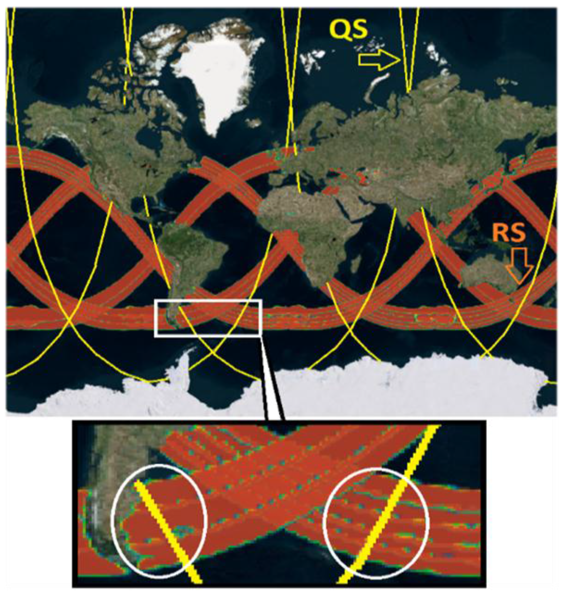
The NSCAT-2014 GMF was deployed to calculate the modeled values at the given sensor parameters (incidence angle and polarization). The single sensor difference between the models and measurements was then subtracted to converge to the double-difference used to cross-calibrate RapidScat and the QuikScat. The double difference calculation process started by loading the measurements and the corresponding instrument configuration within a spatial resolution bin and within the chosen time-difference tolerance. The primary spatial resolution used in this study was a 1° × 1° latitude/longitude grid, with a one-hour maximum interval between overflights, although higher resolutions were investigated with minor effect on calculated cross-biases. To avoid changes in underlying wind conditions, time intervals exceeding one hour were not considered, and we also excluded measurements taken more than one hour from the closest GDAS file. An example of a few RapidScat and QuikScat orbits mapped over the globe are illustrated in Figure 4. The figure shows a wide RapidScat swath (in orange) and narrow QuikScat swath following a non-spinning antenna motor (in yellow). The wide RapidScat swath in the Sun-asynchronous orbit allowed collocation with QuikScat at various local overpass times over the entire swath range of latitudes ±56°.
Gridded overlapping sensor measurements and corresponding configurations (polarization, azimuth, and incidence angle) were passed to the module that uses the GMF to calculate model values. Values of the were calculated from the corresponding GDAS wind fields in those geographical bins containing both RapidScat (subscript RS) and QuikScat (subscript QS) observations, excluding measurements with land or ice flags:
In Equation (1), indicates the incidence angle; denotes the GDAS wind speed; x is the GDAS wind direction relative to the radar azimuth; and P is the radar wave polarization (horizontal or vertical). In the second step, the modeled was compared to the measured to build the bias set where the number of delta points falling into the bin is dependent on the chosen grid resolution:
Equation (2) defines the single difference between the actual sensor measurement and the expected measurement modeled from the GDAS weather data at the given sensor configuration. This difference is calculated for each instrument view taken at different azimuths and polarizations. Values of measured are not averaged within a box. Instead, for each individual measurement, a corresponding modeled is calculated. The 1° grid box is the reference for the underlying GDAS wind vector, so that each modeled in the box uses the same wind vector to calculate the model counterpart to the measured value and enable difference calculation. Once individual differences are calculated, they can be averaged on any desired level: 1° × 1° GDAS box, wind speed range, latitude, polarization, time, etc. Some of the difference statistics are presented in Section 3.
From Equations (1) and (2), the double difference (DD) is the difference between the RapidScat and QuikScat single differences (SD):
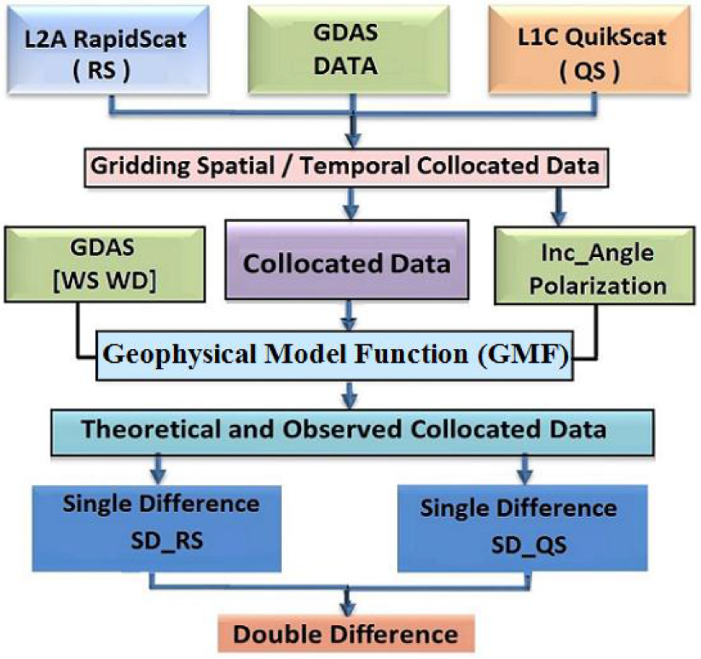
Equation (3) completes the double-difference cross-calibration calculation. Each point represents an individual measured/modeled pair. It was deployed on RapidScat/QuikScat data between January 2015 and March 2016 to compile bias statistics aggregated per time and per sensor variables, as presented in the following section. The entire algorithm is summarized in a block diagram in Figure 5, where WS and WD are the wind speed and wind direction in a 1° × 1° GDAS box, respectively. The collocated data within a box included multiple measurements from both QuikScat and RapidScat taken within a one-hour time interval and within one hour from the GDAS report. It also included the corresponding measurement configurations (azimuth, polarization, and incidence) and a single GDAS wind vector. The single and double difference biases calculated in Equations (1)–(3) may be used to correct measurements and improve the wind retrieval accuracy.
3. Results
This section presents the results obtained after deploying the double difference calibration method across 825 orbits (RapidScat/QuikScat) with GDAS data collected between January 2015 and March 2016. Only sensor measurements within an hour of each of the underlying GDAS grids (0, 6, 12, and 18 Greenwich Mean Time (GMT daily) were considered. The results that follow in this section identified biases between RapidScat and QuikScat, with a general trend of increasing biases in 2016 that coincided with observing a reduced SNR in the RapidScat data.
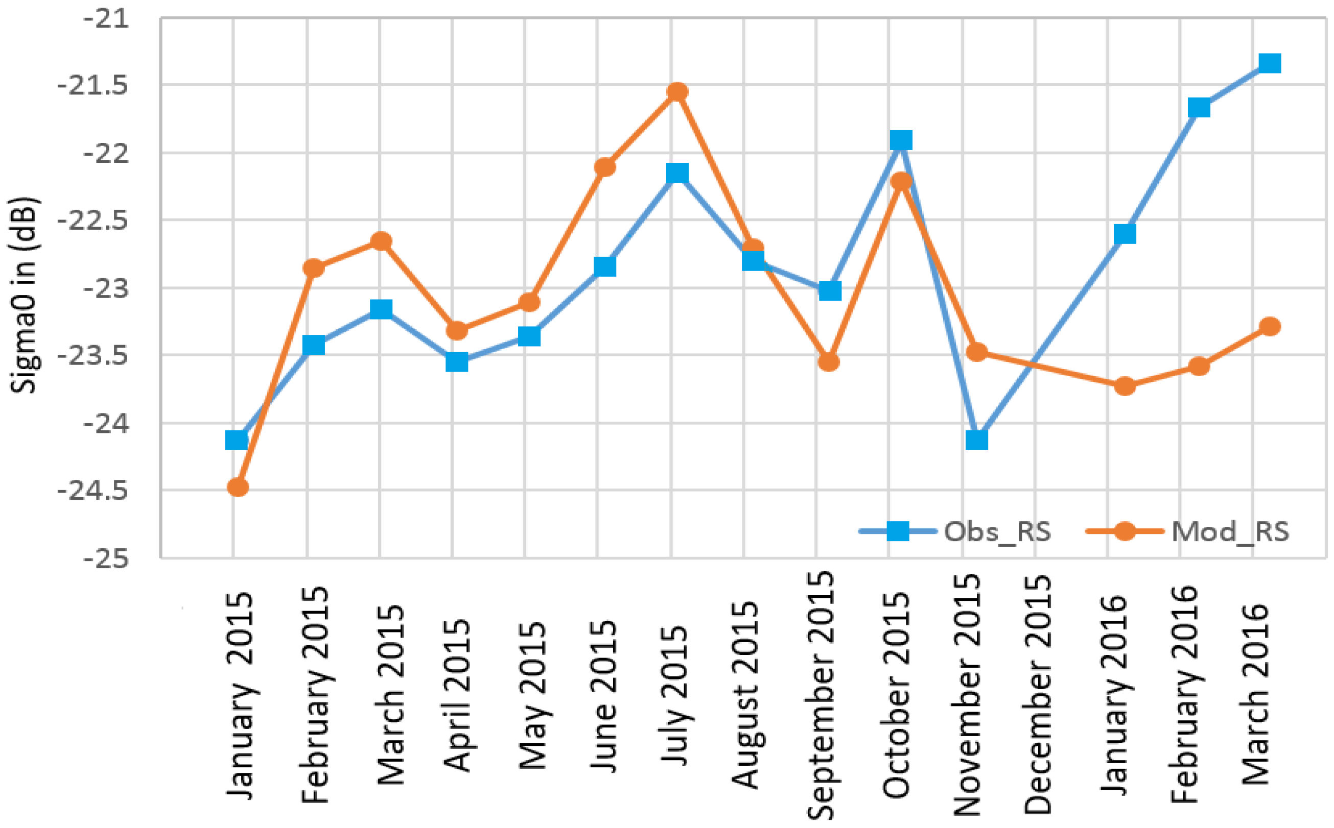
Figure 6 shows the global monthly averages measured by RapidScat and modeled by NSCAT-2014 GMF. Except for the 2016 data, most of the measured data in 2015 showed good overall average agreement, within a range of ±0.5 dB from the model. In 2016, the observed increased faster than the model, resulting in up to a 2 dB single difference bias. It will be interesting to monitor this trend by adding the remaining RapidScat data up to the mission conclusion in August 2016 in a planned follow-up study.
.
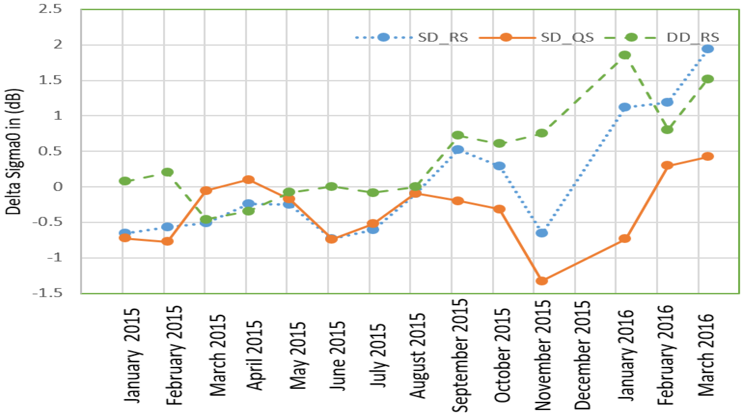
Single differences calculated using Equation (2) for both RapidScat and QuikScat are presented in Figure 7. For most of the processed dataset, overall agreement between the measurements and model was similar for both sensors. Single differences were mostly within 0.5 dB, both absolutely and relative to each other. However, an increase in measured by RapidScat in 2016 was obvious and grew to around a 2 dB bias in January and February. This bias increase coincided with detected periods of lower SNR that were attributed to the receiver gain fluctuations. A correction was applied in the published data products to compensate for the SNR reduction, but the increased bias between the RapidScat and the QuikScat indicated possible insufficient compensation.
Figure 7 also shows the monthly average variations of double differences within 0.5 dB at the beginning of the comparison period, until diverging from August 2015 and approaching the maximum double difference bias of 2 dB in January 2016. The largest discrepancy between the double and RapidScat single difference was recorded in November 2015 at approximately 1.5 dB. Both differences showed a similar trend in the last compared month in March 2016. Moreover, to show the performance of RapidScat for the HH-polarized and VV-polarized measurement separately, it was noticeable that the single difference of RapidScat (SD_RS) biases were higher for vertically-polarized measurements. Monthly averaged (single and double) difference biases are summarized in Table 1. The “Non” label that appears in the double difference rows occurred when the QuikScat was kept at one polarization during that month.
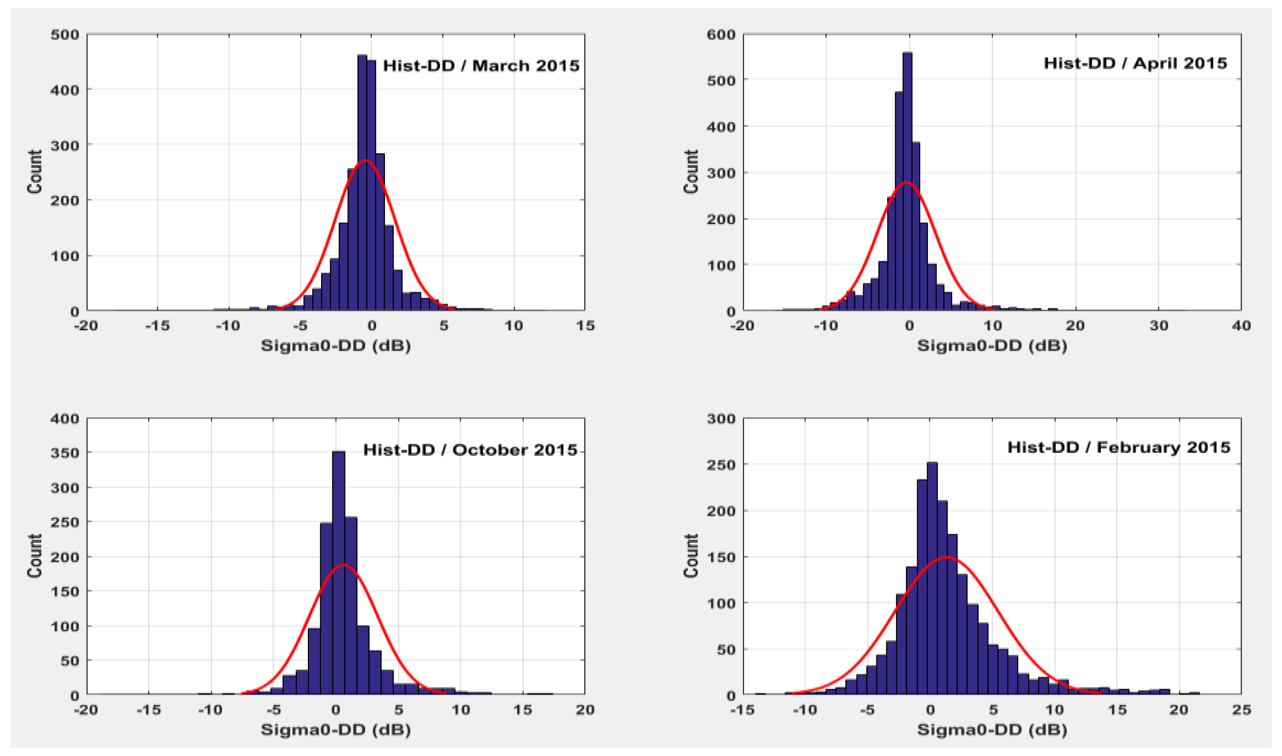
Double difference distributions for selected months are included in Figure 8. Histograms show distributions with a relatively narrow spread around the 0 dB double difference mean until widening in February 2016. Distributions resemble Gaussian probability densities with excess peaks.
The summarizing spread of double difference distributions, and standard deviations of double differences per month are tabulated in Table 2. Variations ranged mostly between 2.0–3.5 dB, until increasing to 5.5 dB in March 2016. Trends visible in Figure 5, Figure 6 and Figure 7 and Table 2 point to a systematic positive bias in RS measurements at the end of the investigation period at the beginning of 2016.
All reported results were calculated at a 1° × 1° latitude/longitude grid resolution. To evaluate the impact of different resolutions, the double difference was recalculated at three additional resolutions: (0.125° × 0.125°, 0.25° × 0.25°, and 0.5° × 0.5°). Figure 9 shows the negligible impact of grid resolution on the calculated double difference.
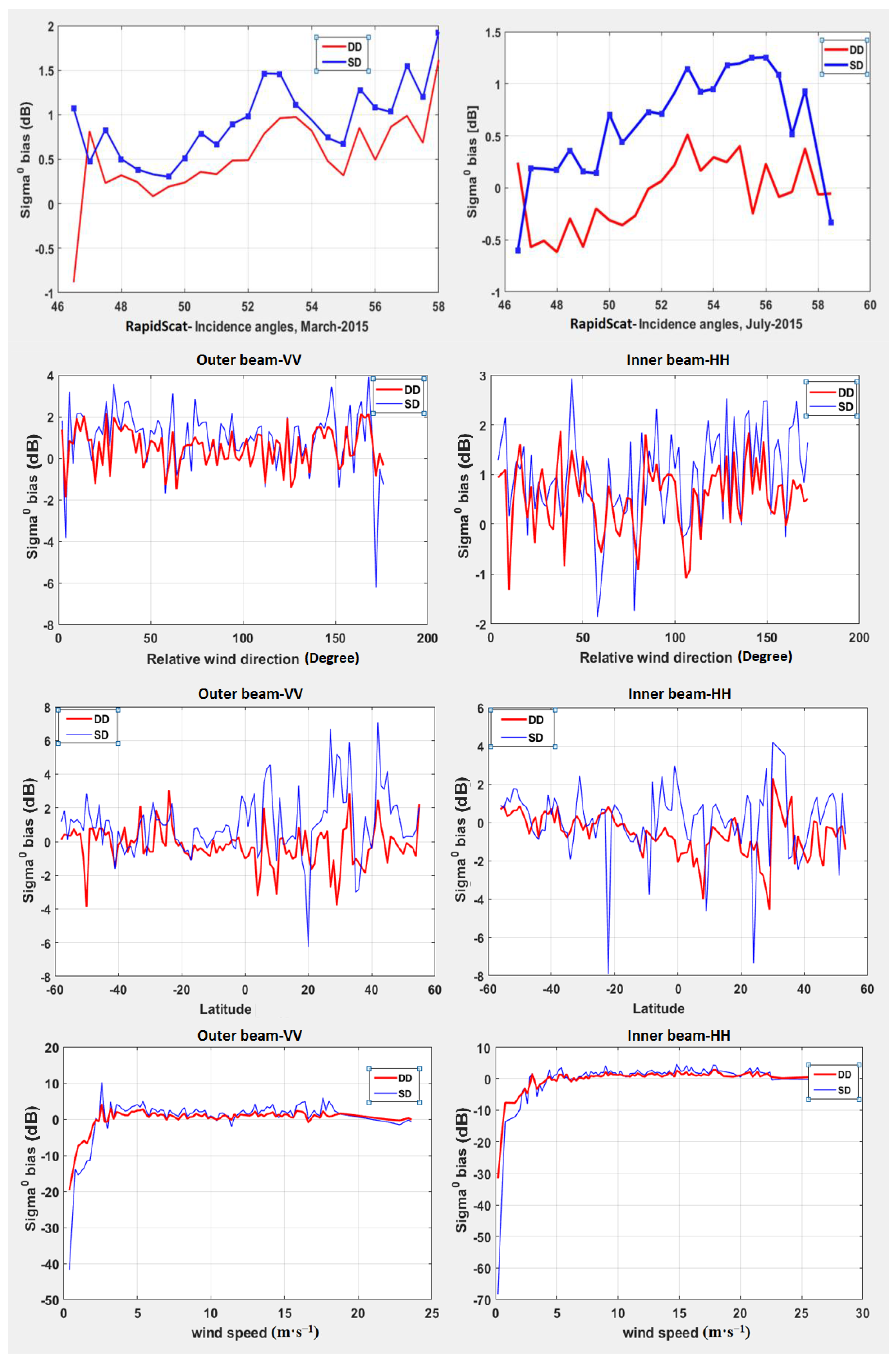
Figure 10 summarizes the monthly bias variations as a comparison of the double and single differences as a function of incidence angle, relative wind direction, latitude, and wind speed. These cases were selected to show the fluctuations of RapidScat single differences and the double difference. Biases were generally centered around 0 dB mean differences. Comparing the double difference (red line) with the single differences (blue line) illustrated the effectiveness of the double difference technique to smooth the single differences. The top panel shows the ability of biases to detect potential bias dependence on the incidence angle for both beams, inner (45°–52°) and outer (52°–58°). The second window presents the average biases as a function of the relative wind direction for both beams, outer (left) and inner (right). Relative wind direction was defined as the difference between wind direction and antenna azimuth angle. Biases at both polarizations followed the same pattern. The fluctuation in both beams was about ±2 dB.
In addition to the incidence angle and wind direction, stability of the biases, as a function of latitude, was investigated to detect potential bias dependency on the latitude. In the results presented in the third window, the horizontal axis represents the latitude over the oceans from 55° latitude-south to 55° north, and the vertical axis presents the averaged biases of both beams, outer (left) and inner (right). The average obtained as the single difference (blue line) was higher than the double difference (red line), with the orbital pattern consistent for different months. Finally, the dependence of the σ° bias on the wind speed was investigated in the bottom window. Significant biases were calculated for both beams, outer (left) and inner (right). The single difference and the double difference showed remarkable agreement beyond 5 m·s−1 wind speed, with biases within 0.5 dB. The instruments at the lowest wind speeds, indicating likely GMF inaccuracies in that range, were below 5 m·s−1, with more than 5 dB.
4. Discussion
In this paper, the double difference technique is applied for the first time to calibrate two satellite scatterometers: RapidScat and QuikScat. It demonstrates RapidScat capabilities to serve as cross-calibration reference for other members of the international scatterometer constellation. In addition to investigating RapidScat bias as a function of individual GMF dimensions (winds speed, relative wind direction, and incidence angle), the impact of the geographical grid resolution on biases was investigated in Figure 9. The grid resolution sensitivity may be explained by the tradeoff between the compensating effects of tighter overlap, as well asthe lower measurement count per bin. While tight overlap reduced the spread, a lower number of points reduced averaging, resulting in a negligible impact of grid resolution on the final result. Therefore, the computationally fastest coarse resolution of 1° × 1° was adopted to report the double difference statistics. The RapidScat calibration and validation study extends bias analysis by adding remaining RapidScat data up to the mission conclusion in August 2016, when the mission effectively ended. Further analysis of the valuable RapidScat measurement set may help estimate the relative validity and stability of other scatterometers that flew simultaneously with sun-synchronous orbits.
5. Conclusions
The double difference methodology, originally derived for radiometers and adjusted for use in scatterometry, was presented. The paper focused on evaluating the long-term stability of the cross-satellite scatterometer validation. Data used in the validation were collected between January 2015 and March 2016. Single and double differences were analyzed through monthly averages as a coarse, but immediate way to evaluate the long-term consistency of two instruments. Results obtained over the 14-month observation period indicated consistency between the two instruments in the first year, until the increased divergence coincided with the detection of low SNR periods in the RapidScat data. Such biases can be used to correct measurements and compare retrievals with and without bias relative to the common reference wind field. Further planned analyses of the RapidScat data will aim to separate biases as functions of additional variables, such as diurnal position, azimuth, etc. These results will be presented in upcoming papers planned in the near future.
Acknowledgments
This research was performed under the grant NNX15AT70G from the NASA Headquarters. Both RapidScat and QuikScat datasets were provided by the NASA Physical Oceanography Distributed Active Archive Center (PODAAC) at the Jet Propulsion Laboratory (https://podaac.jpl.nasa.gov/). NSCAT-2014 GMF was kindly provided by Ricciardulli from Remote Sensing Systems (www.rems.com).
Author Contributions
This research was designed and guided by Josko Zec and W. Linwood Jones. Ruaa Alsabah and Ali Al-Sabbagh performed, analyzed, and discussed the research data. All authors helped in revising and improving this paper, and responding to reviewers comments.
Conflicts of Interest
The authors declare no conflict of interest.
References
- Alsabah, R.; Al-Sabbagh, A.; Zec, J. Calibration of RapidScat Scatterometer. In Proceedings of the IEEE 5th Microwaves, Radar and Remote Sensing Symposium, Kiev, Ukraine, 29–31 August 2017. [Google Scholar]
- Chander, G.; Tim, J.; Hewison, N.F.; Wu, X.; Xiong, X.; Blackwell, W.J. Overview of intercalibration of satellite instruments. IEEE Trans. Geosci. Remote Sens. 2013, 51, 1056–1108. [Google Scholar] [CrossRef]
- Paget, C.A.; Long, G.D.; Madsen, N.M. RapidScat Diurnal Cycles Over Land. IEEE Trans. Geosci. Remote Sens. 2016, 54, 3336–3344. [Google Scholar]
- Rodriguez, E. The NASA ISS-RapidScat mission (Invited). Presented at the American Geophysical Union Fall Meeting, San Francisco, CA, USA, 9–13 December 2013. Paper U23A-03. [Google Scholar]
- Madsen, M.N.; Long, D.G. Calibration and validation of the RapidScat scatterometer using tropical rainforests. IEEE Trans. Geosci. Remote Sens. 2016, 54, 2846–2854. [Google Scholar]
- Biswas, K.S.; Farrar, S.; Gopalan, K.; Santos-Garcia, A.; Jones, W.L.; Bilanow, S. Intercalibration of microwave radiometer brightness temperatures for the global precipitation measurement mission. IEEE Trans. Geosci. Remote Sens. 2013, 51, 1465–1477. [Google Scholar]
- Katsaros, B.K.; Mitnik, L.; Black, P. Microwave instruments for observing tropical cyclones. In Typhoon Impact and Crisis Management; Springer: Berlin/Heidelberg, Germany, 2014. [Google Scholar]
- Zhu, J.; Dong, X.; Yun, R. Calibration and validation of the HY-2 scatterometer backscatter measurements over ocean. In Proceedings of the IEEE Geoscience and Remote Sensing Symposium, Quebec City, QC, Canada, 13–18 July 2014. [Google Scholar]
- Shen, Y. ISS-RapidSca. 2015. Available online: https://www.nasa.gov/mission_pages/station/research/experiments/1067.html (accessed on 20 July 2016).
- RapidScat Project. RapidScat Level 2A Surface Flagged Sigma-0 and Attenuations in 12.5Km Swath Grid Version 1.2. Ver. 1.2. PO.DAAC, CA, USA. 2016. Available online: http://dx.doi.org/10.5067/RSX12-L2A12 (accessed on 20 July 2016).
- Climate Prediction Center. National Centers for Environmental Prediction. National Oceanic and Atmospheric Administration (NOAA). Available online: http://www.ncep.noaa.gov/ (accessed on 20 July 2016).
- Kalnay, E.; Kanamitsu, M.; Kistler, R.; Collins, W.; Deaven, D.; Gandin, L.; Iredell, M. The NCEP/NCAR 40-year reanalysis project. Bull. Am. Meteorol. Soc. 1996, 77, 437–471. [Google Scholar] [CrossRef]
- Crofton, S. Validation of Wideband Ocean Emissivity Radiative Transfer Model. Master’s Thesis, University of Central Florida, Orlando, FL, USA, 2010. [Google Scholar]
- Ghazi, Z. Conae Microwave Radiometer (MWR) Counts to Brightness Temperature Algorithem. Ph.D. Thesis, University of Central Florida, Orlando, FL, USA, 2014. [Google Scholar]
- Ricciardulli, L.; Wentz, F. Progress and future plans on an ocean vector wind climate record. In Proceedings of the IOVWST Meeting, Brest, France, 2–4 June 2014. [Google Scholar]
- Jones, W.L.; Zec, J. Evaluation of Rain Effects on NSCAT Wind Retrievals. Presented at the Oceans 96 Conference, Ft. Lauderdale, FL, USA, 23–26 September 1996. [Google Scholar]
- Jones, W.L.; Park, J.D.; Donnelly, W.J.; Carswell, J.R.; McIntosh, R.E.; Zec, J.; Yueh, S. An improved NASA scatterometer geophysical model function for tropical cyclones. In Proceedings of the 1998 IEEE International Geoscience and Remote Sensing (IGARSS’98), Seattle, WA, USA, 6–10 July 1998; Volume 4, pp. 1994–1997. [Google Scholar]
- Lucrezia, R.; Wentz, F.J. A scatterometer geophysical model function for climate-quality winds: QuikScat Ku-2011. J. Atmos. Ocean. Technol. 2015, 32, 1829–1846. [Google Scholar]
- Ricciardulli, L.; Meissner, T.; Wentz, F.J. Building a Climate Data Record for Ocean Vector Winds. Presented at the American Geophysical Union Fall Meeting, California, CA, USA, 15–19 December 2014. paper OS51D-02. [Google Scholar]
- Ebrahimi, H.; Datta, S.; Santos-Garcia, A.; Jones, L. Radiometric inter-calibration of SAPHIR using the Microwave Humidity Sounders. In Proceedings of the 13th Specialist Meeting on Microwave Radiometry and Remote Sensing of the Environment (MicroRad), Pasadena, CA, USA, 24–27 March 2014; pp. 211–214. [Google Scholar]
- Ebrahimi, H.; Datta, S.; Jones, W.L. Investigation of radiative transfer model effect on radiometric inter-calibration of GPM sounder channels. In Proceedings of the IEEE International Geoscience and Remote Sensing Symposium (IGARSS), Milan, Italy, 26–31 July 2015. [Google Scholar]
- Gopalan, K.; Jones, W.L.; Biswas, S.; Bilanow, S.; Wilheit, T.; Kasparis, T. A time-varying radiometric bias correction for the TRMM microwave imager. IEEE Trans. Geosci. Remote Sens. 2009, 47, 3722–3730. [Google Scholar] [CrossRef]
- Kroodsma, R.; McKague, D.; Ruf, C. Robustness of the vicarious cold calibration algorithm in the double difference method for GPM inter-calibration. In Proceedings of the IEEE International Geoscience and Remote Sensing Symposium, Vancouver, BC, Canada, 24–29 July 2011. [Google Scholar]
- Linwood, J.; Datta, S.; Santos-Garcia, A.; Wang, J.R.; Payne, V.; Viltard, N.; Wilheit, T. Radiometric intercalibration of the Microwave Humidity Sounder on NOAA-18, MetOp-A, and NOAA-19 using SAPHIR on Megha-Tropiques. In Proceedings of the IEEE International Geoscience and Remote Sensing Symposium (IGARSS), Melbourne, Australia, 21–26 July 2013; pp. 1151–1154. [Google Scholar]
Figure 1.
RapidScat pencil beam geometry. (http://winds.jpl.nasa.gov/missions/RapidScat/#instruments).
Figure 1.
RapidScat pencil beam geometry. (http://winds.jpl.nasa.gov/missions/RapidScat/#instruments).
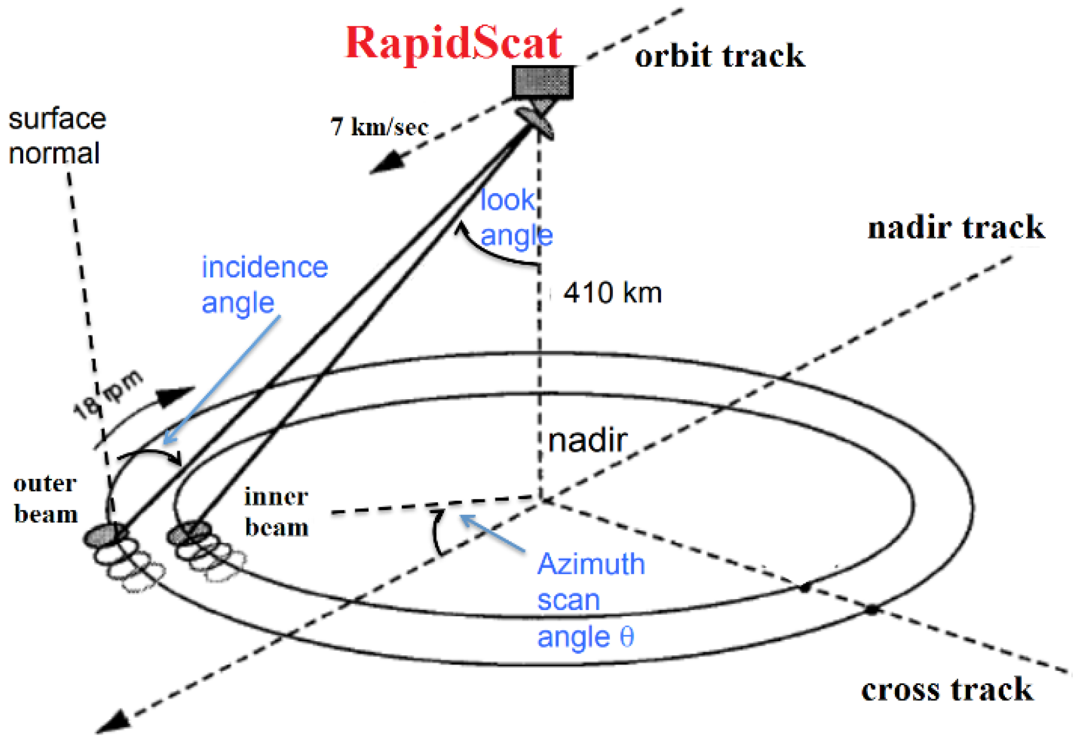
Figure 2.
Wind speed distribution map.

Figure 3.
Example of the modeling via Geophysical Model Function (GMF).
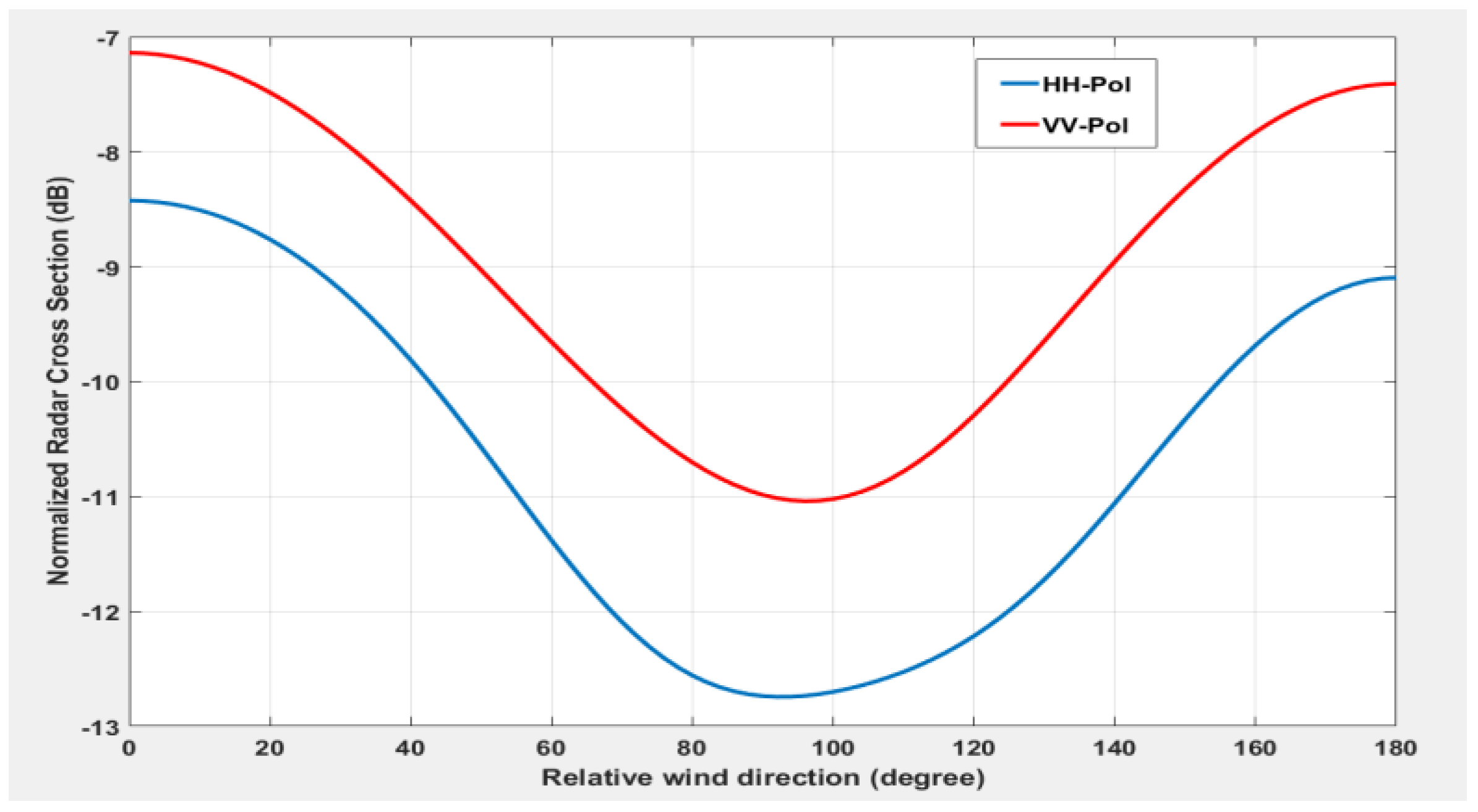
Figure 4.
Global and focused view of the RapidScat/QuikScat collocations.

Figure 5.
Block diagram of RapidScat/QuikScat double-difference calibration.

Figure 6.
Comparison of global monthly average RapidScat measurements and model .

Figure 7.
Monthly average RapidScat/QuikScat single-difference and double-difference.

Figure 8.
Selected monthly double differences (DD) distributions.

Figure 9.
Double difference at multiple grid resolutions.
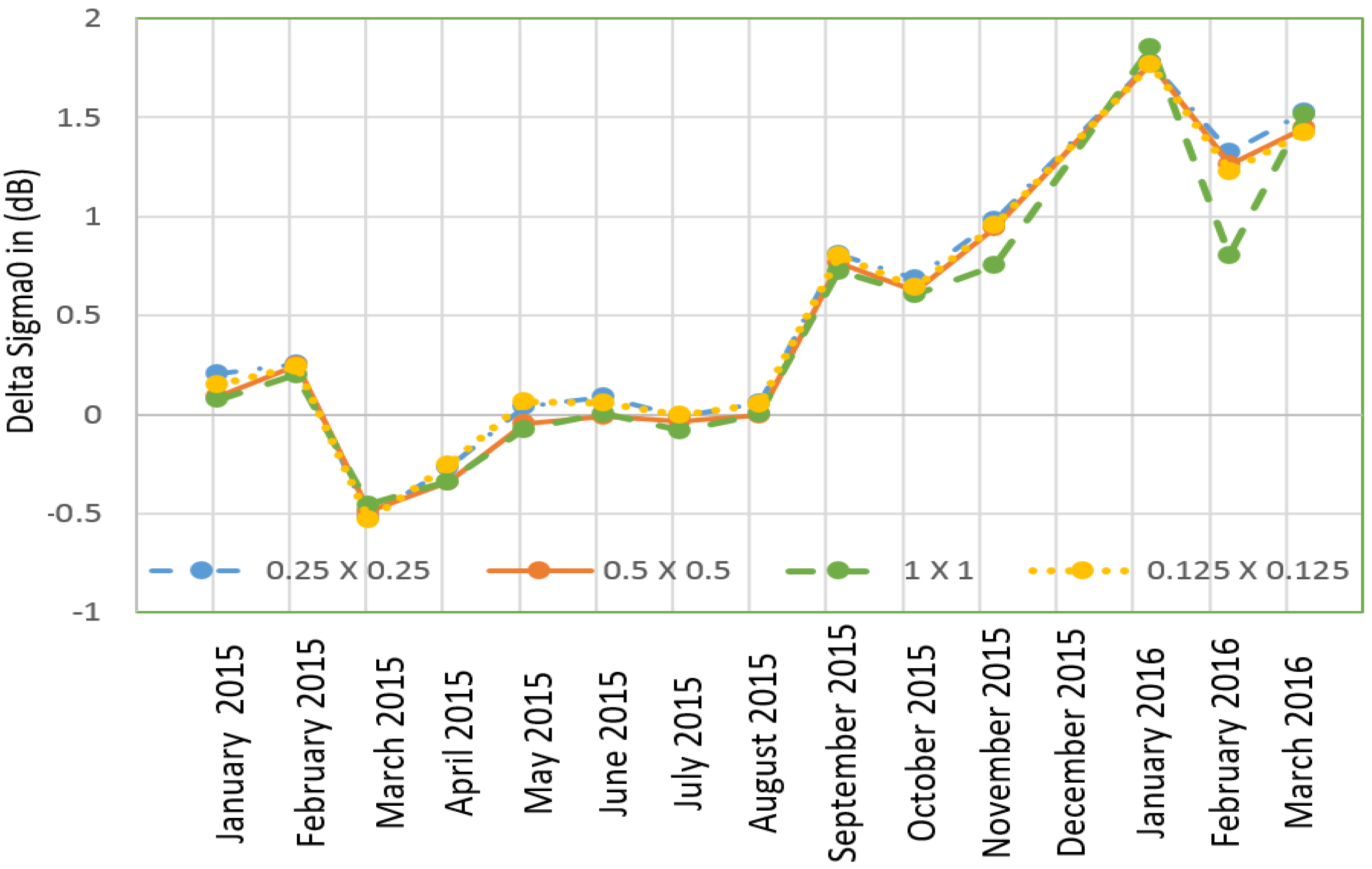
Figure 10.
Comparison of the double and single differences as a function of incidence angle (March and July 2015), relative wind direction (March 2015), latitude (June 2015), and wind speed (June 2015).
Figure 10.
Comparison of the double and single differences as a function of incidence angle (March and July 2015), relative wind direction (March 2015), latitude (June 2015), and wind speed (June 2015).

Table 1.
RapidScat single difference and double difference monthly history for horizontal (HH-pol) and vertical (VV-pol).
Table 1.
RapidScat single difference and double difference monthly history for horizontal (HH-pol) and vertical (VV-pol).
| Months | January 2015 | February 2015 | March 2015 | April 2015 | May 2015 | June 2015 | July 2015 | August 2015 | September 2015 | October 2015 | November 2015 | January 2016 | February 2016 | March 2016 | |
|---|---|---|---|---|---|---|---|---|---|---|---|---|---|---|---|
| HH-POL | SD | −0.18 | −0.55 | −0.6 | −0.12 | −0.26 | −0.7 | −0.63 | −0.26 | 0.34 | 0.15 | 0.53 | 0.79 | 0.5 | 2.14 |
| DD | Non | Non | −0.45 | −0.2 | 0.41 | 0.12 | −0.34 | −0.09 | 0.18 | 0.19 | 0.86 | Non | 0.85 | Non | |
| VV-POL | SD | −0.7 | −0.75 | −0.79 | −0.26 | −0.36 | −0.77 | −0.83 | −0.51 | 0.06 | −0.36 | −0.21 | 0.09 | −0.26 | 1.05 |
| DD | 0.02 | 0.06 | Non | 0.48 | −0.11 | −0.01 | 0.11 | −0.23 | 1.11 | 0.4 | Non | 1.83 | 1.37 | 1.52 | |
Table 2.
Monthly standard deviations of double difference (dB).
| January 2015 | February 2015 | March 2015 | April 2015 | May 2015 | June 2015 | July 2015 |
| 2.0645 | 2.4209 | 2.097 | 3.5033 | 2.28 | 2.2547 | 2.1804 |
| August 2015 | September 2015 | October 2015 | November 2015 | January 2016 | February 2016 | March 2016 |
| 2.5195 | 3.677 | 2.7371 | 2.0645 | 3.3369 | 3.101 | 5.515 |
© 2017 by the authors. Licensee MDPI, Basel, Switzerland. This article is an open access article distributed under the terms and conditions of the Creative Commons Attribution (CC BY) license (http://creativecommons.org/licenses/by/4.0/).
Share and Cite
MDPI and ACS Style
Zec, J.; Jones, W.L.; Alsabah, R.; Al-Sabbagh, A. RapidScat Cross-Calibration Using the Double Difference Technique. Remote Sens. 2017, 9, 1160. https://doi.org/10.3390/rs9111160
AMA Style
Zec J, Jones WL, Alsabah R, Al-Sabbagh A. RapidScat Cross-Calibration Using the Double Difference Technique. Remote Sensing. 2017; 9(11):1160. https://doi.org/10.3390/rs9111160
Chicago/Turabian StyleZec, Josko, W. Linwood Jones, Ruaa Alsabah, and Ali Al-Sabbagh. 2017. "RapidScat Cross-Calibration Using the Double Difference Technique" Remote Sensing 9, no. 11: 1160. https://doi.org/10.3390/rs9111160
Note that from the first issue of 2016, this journal uses article numbers instead of page numbers. See further details here.