Desertification Susceptibility Mapping Using Logistic Regression Analysis in the Djelfa Area, Algeria


1
Faculty of Earth Science, Geography and Land Planning, University of Sciences and Technology Houari Boumediene (USTHB), BP 32 El-Alia Bab Ezzouar, 16111 Algiers, Algeria
2
Helmholtz-Zentrum Dresden-Rossendorf, Helmholtz Institute Freiberg for Resource Technologies, Division “Exploration Technology”, Chemnitzerstrasse 40, 09599 Freiberg, Germany
*
Author to whom correspondence should be addressed.
Remote Sens. 2017, 9(10), 1031; https://doi.org/10.3390/rs9101031
Submission received: 5 July 2017
/
Revised: 28 September 2017
/
Accepted: 4 October 2017
/
Published: 9 October 2017
Abstract
:The main goal of this work was to identify the areas that are most susceptible to desertification in a part of the Algerian steppe, and to quantitatively assess the key factors that contribute to this desertification. In total, 139 desertified zones were mapped using field surveys and photo-interpretation. We selected 16 spectral and geomorphic predictive factors, which a priori play a significant role in desertification. They were mainly derived from Landsat 8 imagery and Shuttle Radar Topographic Mission digital elevation model (SRTM DEM). Some factors, such as the topographic position index (TPI) and curvature, were used for the first time in this kind of study. For this purpose, we adapted the logistic regression algorithm for desertification susceptibility mapping, which has been widely used for landslide susceptibility mapping. The logistic model was evaluated using the area under the receiver operating characteristic (ROC) curve. The model accuracy was 87.8%. We estimated the model uncertainties using a bootstrap method. Our analysis suggests that the predictive model is robust and stable. Our results indicate that land cover factors, including normalized difference vegetation index (NDVI) and rangeland classes, play a major role in determining desertification occurrence, while geomorphological factors have a limited impact. The predictive map shows that 44.57% of the area is classified as highly to very highly susceptible to desertification. The developed approach can be used to assess desertification in areas with similar characteristics and to guide possible actions to combat desertification.
1. Introduction
Desertification is a serious worldwide environmental problem, with consequences with respect to land capacity and biological productivity [1]. It continues to be a major environmental issue in the 21st century [2]. The Convention to Combat Desertification defined desertification as “land degradation in arid, semiarid, and dry sub-humid areas resulting from climatic variations and human activities” [1,3,4]. In this context, the desertification phenomenon was considered by taking into account the degree of vulnerability or the response of the ecosystem [5].
In Algeria, desertification mainly affects the arid steppe areas, which cover a total area of 20 million hectares. These areas are subject to droughts and anthropogenic pressure related to overgrazing and improper land use for agriculture. In recent decades, the widespread degradation of vegetation cover has been determined as one of the main factors causing desertification [6,7,8,9,10]. Today, these areas are in a critical situation. Studies show that about half of these rangelands are desertified or on the threshold of desertification [11,12,13,14,15]. This has led to serious consequences with respect to both the economic and social aspects of development, because these rangelands are used for extensive sheep farming and play a fundamental role in the agricultural economy of the country [10].
Varied and multiple actions have been taken to tackle desertification. To be effective, these actions must focus on the identification of areas that are vulnerable to desertification, the area where it initiated, and its diffusion. Over the last decades, many different mapping techniques have been used for the assessment of desertification, and a large number of studies have evaluated the phenomenon. These studies were mainly based on remote sensing approaches such as change detection using spectral mixture analysis [16,17], multi-criteria evaluation [18], bi-temporal change detection methods [19], a supervised classification approach [20,21,22], long-term study using NDVI, time-trends [23], image differentiation [24], and image rationing [25]. However, change detection techniques face many problems, the most important of which is that observed significant changes may be related to other factors and not to the subject under study [26].
Other approaches have evaluated desertification using key indicators at various geographical scales. The Mediterranean Desertification and Land Use model (MEDALUS), proposed for the first time in 1999 by Kosmas et al. [27], shows clear advantages in comparison with other similar approaches [3,4,5]. The effectiveness of this approach enabled its large-scale use in several Mediterranean countries, including Italy, Algeria, Spain, Portugal, and Egypt. The model identifies areas sensitive to desertification due to a combination of various weighted parameters (i.e., composite indices) such as land cover, geology, soil, climate, and management actions. However, the MEDALUS approach focuses mainly on the physical loss of soil by water erosion in European Mediterranean environments [27], while the phenomenon of desertification in semi-arid areas results from both the natural environment and socio-economic conditions [28].
In this context, we looked for methods that do not require a determined number of variables and provide more freedom to introduce new variables, in particular socio-economic factors. Additionally, it is more important to assess desertification and identify responsible factors than to only evaluate sensitivity.
We thus applied logistic regression, a multivariate statistical method which has been widely used to predict a categorical outcome, using many causality predictors [29]. Being simple to use, it has become a widely accepted method for a broad range of scientific disciplines. Logistic regression has been applied in the field of remote sensing for change detection in land cover [30] and for insect tree defoliation mapping [31]. Logistic regression techniques have also been used in ecology, particularly for conservation planning and wildlife management [32,33]. In earth sciences, logistic regression analysis has been implemented with different goals, for example in soil-landscape modelling [34] and prediction of post-fire soil erosion [35], and it has been extensively used for landslide susceptibility mapping with various techniques [36,37,38,39,40]. Our choice was based on the fact that both desertification and landslides are natural hazards controlled by numerous variables and are characterized by non-linearity.
The aims of this study were to apply the logistic model to identify the most susceptible areas to desertification in a central part of the Algerian steppe, and to evaluate and provide an explanatory model of key factors associated with desertification. To achieve these objectives, we used three main steps. The first step involved the identification and extraction of the predictive factors related to desertification based on the characteristics of desertified areas. The second step was to determine the best predictive model. The third step was to evaluate the contribution of each factor to the phenomenon and determine the most influential factors. Finally, the quality of prediction and the stability of the model were evaluated using two validation methods: the area under the receiver operating characteristic (ROC) curve and the uncertainty measure.
This work stresses that an accurate desertification susceptibility map, associated to an explanatory model of key factors, provides a reliable tool for desertification risk mitigation. Such tools are helpful in the planning phase of developmental activities and to take appropriate preventive measures. This can also be extended to guide possible actions to combat desertification in similar areas.
2. Study Area
The study area lies between latitudes 6°29′ and 5°36′N, and longitudes 35°15′ and 34°41′E, covering an area of about 4097 km2 in the central part of Algeria, in a transition area between the Hautes Plaines region and Saharan Atlas Mountain (Figure 1).
The climate is semi-arid and is strongly marked by a continental influence, with cold, wet winters and hot, dry summers. Rainfall is scarce and irregular, with an average annual rainfall that ranges between 200 and 400 mm. Precipitation usually occurs in the form of thunderstorms and torrential rain, sometimes mixed with hail. The number of rainy days varies between 37 and 80 per year. The average evaporation exceeds 2450 mm/year. The average annual temperature is generally greater than 20 °C. The minimum temperature in the coldest month is 1.9 °C, while the maximum temperature in the warmest months can exceed 37 °C [41,42]. The number of days of frost can reach 40 per year. The prevailing winds are mainly from the west and northwest in winter and the southwest in summer. The mean wind speed is 2.7 m/s [43]; winds are sometimes violent due to the amount of open space without any physical obstacles.
Soils are characterized by the presence of limestone accumulation and low organic matter content [10]. These soils are generally shallow, however some soils located in depressions are relatively deep and rich.
The vegetation consists mainly of patches of grasses that do not fully cover the ground, such as Alfa (Stipa tenacissima), and white Wormwood (Artemisia herba alba) [41]. These perennial grasses occupy a large part of the territory, especially in the South. The forests which occupy the mountain ranges are bright and airy. The main tree species are the Aleppo Pine, Holm oak, and the Phoenician Juniper. Rangeland also covers an important part of the area of study [44].
3. Methodology
3.1. Methods
The selection of an appropriate model is subject to the nature of the dependent and independent variables. In a linear regression model, the dependent variable must be continuous. However, the phenomenon of desertification is dichotomous and is best described by multivariate statistical models, such as logistic regression or discriminant analysis [45]. In this study, we applied logistic regression, which describes the relationship between a dependent variable (the response factor) that is usually the occurrence or not of an event, and several independent variables (the predictive factors) that influence the occurrence of this event [46]. Logistic regression has been frequently used in many fields such as social, health, and earth sciences as well as ecology.
In our case, logistic regression was simpler to use compared to discriminant analysis because of the mixture of numerical and categorical variables. The logistic regression model can automatically generate necessary dummy variables [37]. Also, discriminant analysis requires a normal distribution of independent variables, which is not always available for natural data originating from, for example, land use and land cover [45].
Additionally, many researchers have preferred to use logistic regression due to its similarity to linear regression as it relies on simple tests [37,45], while adding a function that allows prediction of the probability of the event and describes complex nonlinear relations that often characterise natural phenomena. Logistic regression also allows for estimation of the odds ratio, which provides information on the strength and direction of the association between the dependent variable and the independent variables [47].
In our situation, the independent binary variable was used to present the presence or the absence of desertification. The logistic model can be expressed in its simplest form with the following equation:
where is the probability of desertification occurrence that varies from 0 to 1 on an s-shaped curve, and is the linear logistic model, which varies from to , and can be defined as:
where α is the intercept of the model, (i = 1, 2, 3, …, n) are the estimated slope coefficients of the logistic multiples regression model, and (i = 1, 2, 3, …, n) represents the independent variable.
The logistic model for desertification can be represented as:
Logistic regression looks for the “best fit” equation as in linear regression, but with a different method. Instead of using the least-square method for best fit, it uses the maximum likelihood method [37]. The unknown values of α and are estimated using the data of the independent variables. The observed data in each pixel either have a value of 0, meaning the absence of desertification, or 1, meaning the presence of desertification. With these estimates, we calculated the probability of the desertification for the remaining pixels, using the observed values of the independent variables [45].
3.2. Causal Factors and Desertification
Predictive factors used to assess desertification may vary from one region to another. For this reason, we tested a set of key factors that provide information about desertification commonly used in the literature [3,5,27,28] and we then selected those that seemed to be most adequate for our study area. We also faced constraints related to the lack of data in countries subject to desertification [48], and attempting to compensate for this deficit by using remote sensing data is a useful tool for mapping many factors.
Sixteen predictive factors were selected as potential determinants of desertification and prepared as thematic layers. These factors belong to one of the following four categories: soil, geomorphological, environmental, and socioeconomic factors.
All maps of the factors were converted to the same pixel size equalling 30 m, similar to the resolution of maps derived from Landsat 8 imagery and SRTM DEM.
The logistic model used in this study can process continuous or categorical data, or both. The categorical form factors include land cover, slope aspect, and lithology. The others factors, such as slope and elevation, have a continuous form.
Categorical variables should be encoded in order to create a new set of dummy binary variables for each class of the categorical variable [37,38,49]. A value of 1 is assigned to the target class, and the value 0 is assigned to the other classes. Each categorical factor generates a number of binary maps equal to the number of classes contained in this factor. For example, 15 binary maps were produced for the land cover map, which contains 15 classes.
3.2.1. Soil Factors
Soil is an important factor in semi-arid zones. Desertification will proceed when the soil depth is not capable of sustaining a certain minimum of vegetation cover [27]. Due to the absence of data regarding soil characteristics, such as texture, soil depth, and organic matter, we used a lithological map to obtain properties of the rocks and their susceptibility to desertification. The lithological map study involved eight lithological units provided by the National Agency for Regional Planning—Algeria [50].
Land surface temperature (LST) is also an important parameter in the physics of Earth surface processes [51], and can be used to explain the dynamic of desertification [52,53]. LST is estimated using thermal bands 10 and 11 of the Landsat-8 Thermal Infrared Sensor (TIRS). We applied a method widely used to calculate the LST [54], based on the estimation of land surface emissivity extracted using the NDVI. We used an image acquired in May 2015, the same image that was used for the extraction of the NDVI.
The following equation was used to calculate the LST:
where is the at-satellite brightness temperature, calculated from the radiance which was derived from the digital number according to United States Geological Survey USGS methodology [55]. is the wavelength of the emitted radiance (11.5 um). For = h × c/ (1.438 × 10⁻² m K), h is the Planck constant (h = 6.6261 × 10⁻³⁴ Js), is the Boltzmann constant ( = 1.3806 × 10⁻²³ J/K), c is the speed of light (c = 2.9979 × 10⁸ m/s), and (ε) is the land surface emissivity, calculated using the NDVI image [56,57].
3.2.2. Geomorphological Factors
In order to assess desertification, previous studies have identified a wide range of factors related to landform characteristics [3,4,58,59,60,61,62]. Among those, geomorphological characteristics play an important role in desertification processes [63,64] and identifying desertification through wind and water erosion in dry areas is relatively easy [63,65]. In this category, six predictive factors which describe the morphology of the landscape were used.
Elevation is an influential factor in the erosion of the landscape [27]. In this study, elevation was derived from the new digital elevation model from the Shuttle Radar Topography Mission, known as “SRTM Plus V3”, with a resolution of 1 arc-second (~30 m) [66]. Elevation was used to create the other geomorphological factors.
The TPI compares the elevation of each pixel to the average elevation of the surrounding pixels [67]. A positive TPI value means that the area is located higher than its average surroundings, as with ridges for example. However, negative values mean that the area is lower than the average, for example in the case of a valley floor [68]. The TPI is calculated with the following equation [68,69]:
with being the elevation of the central pixel, and the average elevation around it. We executed an algorithm in the QGIS processing toolbox in order to compute the TPI for the study area, and we used a moving window of 10 pixels.
The hypsometric integral (HI) helps to estimate the erosional status of a watershed [70,71], and is inversely correlated with the amount of material removed by erosion [72]. The lowest values of HI (HI < 0.35) are commonly found in long-lived landforms, where the average topography is low and a few relict highs, such as inselbergs or mesas, are preserved. In contrast, the highest HI values (HI > 0.6) are found in young or rejuvenated landscapes, where the average topography is high and incised by an entrenched drainage system. Average HI values (0.35 < HI < 0.6) are found in mature landforms associated to a set of concave or V-shaped valleys [73]. The hypsometric integral is calculated using the following equation [74]:
with hmean, hmin, and hmax being the mean, minimum, and maximum elevations of the analysed area, respectively.
Slope gradient and slope aspect are key factors that control soil erosion [75] as well as the types of cultivation, and determine the grazing areas [76]. The slope aspect notably influences the local environment [77] and is considered an important factor for land degradation processes, which affect several elements such as temperature, evaporation, and vegetation [78].
Curvature illustrates a line formed by the intersection of a plane with the land surface [79]. Its importance lies in the fact that the susceptibility of the terrain to erosion varies depending on the curvature [80]. A negative value means that the surface is locally convex, a positive value means the surface is locally concave, and a value of 0 means that the surface is flat [39,68].
3.2.3. Environmental Factors
Environmental factors play an important role in the desertification process [64]. Past studies showed that land cover, drainage, and climatic conditions are indicators that allow the characterization of soil conditions during erosion and processes associated to desertification [28,59,81].
Six parameters were used as environmental predictive factors of desertification: precipitation, NDVI, land cover, drainage density, distance to drainage, and evapotranspiration.
In the absence of reliable and accurate precipitation data from climatological stations, we chose to work on two types of data. The first is the decadal rainfall isohyets map provided by the National Agency of Water Resources—Algeria, published in 2002 [82]. The second precipitation data was derived from the Tropical Rainfall Measuring Mission (TRMM). These data have been widely used with good performance [83,84]. We used an average monthly pixel-based precipitation rate with a spatial resolution of 0.25 degrees (3B43 v7) which spans a period of 17 years (1998–2014).
The NDVI has been widely used as an indicator to assess and monitor land cover change and desertification [23,60,85]. NDVI was obtained from the reflectance (ρ) of the Landsat 8 image acquired in May 2015 (level 1A) which was completed after atmospheric correction using the Fast Line-of-Sight Atmospheric Analysis of Spectral Hypercubes (FLAASH) model.
Land cover information was extracted with 15 classes from the map produced by the High Commissariat for Steppe Development [86]. Drainage conditions were largely used as influential parameters to evaluate desertification [28,60].The drainage density was calculated from the drainage network with a 100-pixel radius circle, using a 30-m resolution SRTM DEM [68]. Buffer zones around the drainage network were used to derive the distance to drainage. The extraction of these drainage parameters was performed using the TecDEM toolbox.
3.2.4. Socioeconomic Factors
Desertification is associated with the natural environment as well as socio-economic conditions [28]. Several attempts have been made to integrate the socio-economic aspect to assess desertification [91,92,93,94]. According to a new desertification paradigm which must take into account the socio-economic dimension [48], we tried to include two socio-economic indicators that are related to the phenomenon of desertification.
Overgrazing is a clear cause of desertification [92] and is one of the factors responsible for degradation in our study area [7] due to the importance and number of livestock. In the absence of a livestock distribution map, we calculated the livestock density by dividing the number of livestock by the surface of the rangeland for each municipality in the study area. We used the numbers of livestock declared by the agricultural services directorate of the Djelfa province in 2014.
The increase in rural population density also leads to land degradation [95], putting more pressure on pastures, and cropland expansion. In the absence of recent statistics for the rural population, we estimated numbers for 2015 with the geometric method [96], by using the growth rate observed between the last two population censuses of 1998 and 2008. Afterward, we calculated the density by dividing the rural population number by the area of rangeland for each municipality in the study area.
3.2.5. The Desertification Inventory Response Factor
The dependent variable used to evaluate the logistic model is the susceptibility to desertification. We focused mainly on areas that are characterized by an advanced degradation of vegetal cover because it is the most important aspect of desertification in the region [6,7,8,9,10]. In the absence of updated maps that indicate the distribution of desertified areas, we exploited the detection change map between 1984 and 2014 produced by Djeddaoui et al. [97] as a guide to selecting large areas where change existed. Both desertified and non-desertified zones were mapped during fieldwork carried out between April and May 2015. The criteria adopted in our study to discriminate desertified and non desertified areas was the degree of land degradation. The scale extends from the advanced vegetal cover degradation to the appearance of sand. This task was supplemented by the interpretation of Google Earth images. In total, 139 desertified zones were mapped in the study area, with measurements varying between 0.10 and 55.91 hectares. We followed a north–south gradient in order to take into account all types of geomorphological sets and climate change. The raster data of desertified zones consist of 8439 pixels measuring 30 m in size.
3.3. Input Database for Logistic Regression Analysis
To estimate the coefficients of the logistic model, we created datasets containing the values of the independent variables and the status of the dependent variable for the same pixels.
To generate the desertification susceptibility map, the logistic regression model needed pixels with or without the presence of desertification [49]. Several methods of sampling are used for susceptibility. Many studies confirm that the best sampling method is when the ratio of pixels with desertification to pixels without desertification is equal to 1 [38,98,99]. Thus, we used the same number of samples for both the presence and absence of desertification.
Pixels with desertification were randomly subdivided into two sets. The training data set for the regression analysis included 69.45% of the pixels (5861 pixels), and the validation data set for accuracy assessment included the remaining 30.55% (2578 pixels). We then selected a number of pixels without desertification that was equal to the number of pixels with desertification, reaching a total of 8439 pixels. These pixels were also subdivided into training and validation datasets (69.45% and 30.55%, respectively). Thus, the final database consisted of 16,878 pixels.
We prepared a table containing an equal number of desertified and non-desertified pixels. The first column contained the status of the dependent variable to desertification for the 11,722 analysed pixels. A value of 1 was assigned if the pixel was desertified and 0 otherwise. The other columns, one per independent variable, contained the values of the independent variables for the 11,722 pixels.
The logistic regression analysis was performed using the R package “stats” [100]. Output α and β values were used to calculate the linear logistic model z.
Finally, we introduced the input file for logistic analysis as a data table, which was analysed with R software to extract the value α and β of the model, and could then be used to calculate the value of z.
3.4. Variables Selection and Model Development
Using statistical tests, we checked if the independent variables would affect the predictive variable or not, so that only significant variables would be retained in the logistic regression analysis. We performed a bivariate analysis to verify the relationship between the dependent variable and each independent variable; all non-significant associations with p > 0.05 were excluded from the model. This analysis allowed us to exclude variables that presented a singularity, which is a type of redundancy that appears after the creation of the dummy variables. We used Pearson’s chi-squared (χ2) test to evaluate the relation for the qualitative variables, and the Student’s t-test for the qualitative variables [101].
Prior to obtaining the final model with significant variables, building a number of models with the largest possible number of independent variables is preferable in order to check which variables are significant in the model with the presence of all other variables [102].
In this study, backwards selection was used. The input variables were performed manually, based on introducing the variables one by one. We did not use the automatic method because it selects the predictors only on the basis of statistical criteria. This type of selection is preferable when the search field is less explored and the knowledge of the effect of each independent variable is limited. Moreover, it is highly sensitive to the multicollinearity [102,103]. After entering each variable, the Wald statistics were computed to check the contribution of individual predictors in the model. We generally kept all variables with a p-value < 0.05 [38,40,47]. In other words, we accepted these independent variables as influential predictors.
In order to ensure that we considered the least number of all significant variables, the resulting model was tested again based on the significance of the likelihood ratio. During this step, we entered and removed variables. After each entry, we calculated the likelihood ratio for both models. If there was a significant change between the two likelihood ratios, (where the p-value was less than 0.05), the first model was kept without changes [40,104].
The goodness of fit of the model was also evaluated using Cox and Snell, and Nagelkerke pseudo R2 tests [105], which are similar to the coefficient of determination R2 in ordinary linear regression. The Cox and Snell pseudo R2 value did not exceed 1. Nagelkerke’s pseudo R2 is a better version of the Cox and Snell pseudo R2 and is often preferred because its value varies between 0 and 1 [40,105]. Usually a R2 value higher than 0.2 indicates a relatively good fit [106].
The adjustment of the logistic regression model is generally sensitive to collinearity between independent variables [46]. Multicollinearity poses a problem because it increases the variance of the regression logistics coefficients. The variance inflation factor (VIF) is usually used to check the multicollinearity diagnosis. In our study, we calculated the VIF for each variable. If the value was greater than 1.5, the variable was excluded from the model [38,107].
3.5. Model Prediction and Uncertainties
Model validation is a key step and helps to evaluate the reliability of the model before it can be used for practical applications.
In order to assess the accuracy of the model, we used a quantitative measurement method, called the area under the ROC curve, on a separate desertification validation set involving 30% of the total desertification pixels. The area under the ROC curve is commonly used as a metric to measure the goodness of a susceptible model [45,68,108,109]. A large area under the curve indicates good model performance. The curve is a two-dimensional plot where the y-axis represents the probability of a correctly predicted response to an event in terms of sensitivity or true positive rate, and the x-axis represents the probability of an incorrect predicted response to an event, in terms of specificity or false positive rate [40]. If all desertified areas are correctly predicted, the area under the curve will equal 1, but in general an area under the curve greater than 0.5 is acceptable [110,111,112,113].
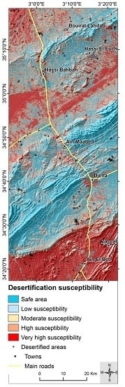
To facilitate the interpretation of the results for users and to help the decision-maker to take the appropriate action to combat desertification, we classified the desertification susceptibility map based on the literature. In previous studies, the number of susceptibility classes varied commonly from two to five [68,107,114]. In order to align the results of our study with other prior studies on desertification, the probability map was divided into five susceptibility classes: very high, high, moderate, low, and safe. In this study, we used natural breaks classes based on the Jenks optimization procedure. This procedure determines the best arrangement of values into several classes that maximizes between-class variance and minimizes within-class variance [115,116].
Uncertainty is an important test that has been applied by different researchers to measure the quality of susceptibility mapping [68,117,118]. First, we tested the sensitivity of the model to the changes in the input training dataset using a bootstrapping technique. Fifty desertification susceptibility maps were generated using 50 different training datasets that were randomly selected, involving 70% of the pixels with desertification. For each map, we kept the same predictive factors of the resulting model. Then, we calculated the area under the ROC curve for each of these 50 maps, using the validation datasets involving 30% of pixels with desertification. The sensitivity of the model was represented by a box plot diagram, which expresses the variation of the area under the ROC curve.
The second measure of uncertainty included the estimation of the model’s error. For this purpose, we randomly selected 20,000 pixels. For each model, we obtained descriptive statistics, including the mean and standard deviation from the 50 estimated susceptibility maps using these selected pixels. For each model, we calculated the mean and standard deviation. The error plots show the mean value in the x-axis against their two standard deviations of susceptibility estimates in the y-axis. [68,117,118].
4. Results
4.1. Evaluation of Predictive Factors
In order to clarify the characteristics of the desertified areas, we evaluated the relationships between the desertified area, represented by the training and validation datasets, and desertification-predictive factors.
The NDVI was between −0.54 and 0.92 in the area study. Desertified areas had values between 0.08 and 0.29, and more than 96% of the desertified areas had an NDVI value below 0.22 (Figure 2B). The study area included 12 types of land-cover/use: agriculture, grazed cropland, sebkha, rangelands, forest, afforestation, esparto grass, dunes, uncultivated areas, urban areas, and cultivated rangelands. Over 64% of the desertified areas were found in rangelands, and 20% of desertified areas were found in agricultural zones (Figure 2E).
Over 43% of the desertified areas were found in areas with annual precipitation below 300 mm, and that percentage rose to more than 98% for areas with less than 400 mm of annual precipitation (Figure 2A). The study area contained eight types of lithostratigraphic units: alluvium, conglomeratic clay-sand formations, lacustrine and limestone, clay, schist-marl, a few limestone and gypsum intercalations, massive limestones in banks or platelets, alternating sandstone and clay, chotts, and sand (Figure 3E). Alluvium, clay, and alternating sandstone and clay constituted more than 79% of the total desertified areas.
The drainage density had a range from 0.64 to 3.03, and for the study area, desertification occurred in the range 1.25–2.85 (Figure 2G). Over 55% of the desertified area was characterized by low drainage density, and 44% with moderate drainage density.
We found that over 17% of the desertified areas were less than 100 m from drainage, but the highest density of desertified areas, with over 72%, were between 100 and 400 m from drainage. The rest of desertified areas, about 10%, were within a distance of more than 400 m from drainage (Figure 2F).
For the slope aspect, the percentages of desertified areas for the six faces—west, northwest, north, northeast, east, and southeast—ranged between 10.17% and 12.18%, and increased to more than 14% for the south or southwest faces. The flat face had the lowest percentage of desertified areas, at 2.90% (Figure 3H).
The TPI ranged between −79.25 and 52.37 m over the entire study area and between −9.56 and 8.78 m for the desertified areas (Figure 3G).
For the entire study area, the slope gradient ranged from 0 to 68.94; the maximum slope gradient for desertified areas was 20.8 degrees. Over 84% of the desertification area was characterized by a slope of less than five degrees (Figure 3F).
The elevation of the desertified areas ranged between 750 and 1370 m (Figure 3B), and the central part of the study area included the highest areas. There was no clear link between the distribution of desertified areas and elevation. However, about 60% of the desertified area was located at altitudes below 1000 m.
The HI ranged between 0.5–0.75 (Figure 3C), and 93.89% of the desertified area had a value ranging between 0.35 and 0.6 in an equilibrium situation.
The curvature ranged between −19.33 and 24.44 for the entire study area. However, for desertified areas, the value ranged between −2.77 and 2.0, with about 41.34% having a negative value, and more than 45 had a positive value (Figure 3D).
The LST map had a range between 20.92 and 44.64 °C for the entire study area (Figure 3A), while the desertified areas were characterized by a temperature between 32.56 and 42.50 °C.
While the annual evapotranspiration range was 1300–1700, about 33% of desertified areas were characterized by evapotranspiration of less than 1500 mm and this value increased to more than 98% if the evapotranspiration was less than 1600 mm (Figure 2H).
The livestock density in the total study area ranged between 0.48 and 32.88 units per hectare. Over 80% of the desertified areas had a density of between 0.48 and 9.94 units per hectare (Figure 2D).
The rural population density ranged from 0.07 to 1.48 inhabitants per hectare in the desertified areas (Figure 2C).
4.2. Selected Variables and Desertification Probability
The regression analysis started with 45 prediction factors, including continuous factors and the classes of the categorical factors, as shown in Table 1.
We completed a bivariate analysis to check the relationship between the response variable and each predictor variable. Thus, we retained only the significant variables that had a p-value < 0.05, and excluded seven predictor variable units, including the northeast aspect, the flat aspect, LST, curvature, dunes, uncultivated areas, and chotts. We used the decadal data as the precipitation factor because the TRMM data were not significant.
The next step started with the base model which contained only the response factor. The 39 predictor variable units were successively introduced. At the same time, we controlled any significant changes and 25 factors were considered as non-significant (p-value < 0.05) and were subsequently removed from the model.
In the same way, every time we added a predictor factor, we controlled the values of VIF in order to avoid the problem of multicollinearity, and any variable with a VIF of less than 1.50 was excluded from the logistic analysis (Table 2).
We also calculated the Cox and Snell and Nagelkerke pseudo R2 (Table 3). For the final model, Cox and Snell and Nagelkerke pseudo R2 values were 0.40 and 0.53, respectively, which indicated that the predictor variables could explain the response variable.
In the end, the 13 factors that were accepted as being influential predictors, with a p-value <0.05, were: south aspect, northwest aspect, rangelands, grazed cropland, cultivated rangelands, slope, NDVI, TPI, HI, precipitation, drainage density, dunes, and massive limestones in banks or platelets (Table 4). The predictor variables that had an odds ratio equal to one were neutral in assessing the desertification susceptibility. The predictor variables that had an odds ratio greater than one were positively related with desertification susceptibility. They included south aspect, rangelands, grazed cropland, cultivated rangelands, TPI, dunes, massive limestones in banks or platelets, and drainage density. The predictor variables that had an odds ratio of less than one had a negative relationship with desertification susceptibility. They included slope, NDVI, HI, precipitation and northwest aspect (Figure 4).
The class of rangelands and the NDVI had odds ratios of 2.22 and ~0, respectively, and so they appear to be the main predictive factors, with a stronger effect on desertification than any other factor.
Our results confirmed that desertification is a complex phenomenon controlled by numerous natural and human factors. Land cover factors play a major role in determining the occurrence of desertification. Climatic factors had the next most influential role, while geomorphological factors had a lower predictive value. Interestingly, variables that have a relationship with water erosion do not appear to play a major role in desertification. However, this does not negate the importance of other forms of erosion.
Finally, we calculated the predicted probability of desertification for the entirety of the targeted area, observing the values of the predictor variables by using Equation (3). For each pixel, we added the values of the products of the predictor variables with their estimated coefficients (). We then added the intercept value (α), and the probability of desertification was obtained.
The result was a raster map with the pixel value representing the estimated probability of desertification, which varied from zero to one. The desertification probability values were divided into five classes (safe, low, moderate, high, and very high) to generate a desertification susceptibility map (Figure 5 and Table 5). These classes cover 23.99%, 16.83%, 14.62%, 15.35%, and 29.22% of the land area, respectively.
5. Discussion
5.1. Model Validation
This study, being different from previous studies on the evaluation of sensitivity to desertification, statistically evaluated the quality of prediction and the stability of the resulting model. In order to verify the predictive skill of our model, we used area under the ROC curve as a quantitative measurement to estimate the model’s accuracy. The ROC curve for the model used in this study is shown in Figure 6A. The area under the curve is 0.878, equivalent to an accuracy of 87.8%. Hence, this shows that the model used in this study demonstrated reasonably good accuracy in predicting the susceptibility to desertification.
To test the stability of the model, we conducted an uncertainty measure. Figure 6C shows that the model is characterized by less error; the two standard deviations of the obtained probability estimate are less than 0.04. All values were distributed in a bell curve shape, and we found that the measure of two standard deviations was very low (<0.02) for areas classified as highly susceptible (probability > 0.84) or classified as a safe area (probability < 0.15). The obtained estimate of the extreme values is less variable, and therefore reflects the reliability of the model. For the intermediate values, with a probability between 0.37 and 060 for moderate susceptibility, we found that the measure of two standard deviations increased slightly to less than 0.04, which reflects the degree of variability, and this usually characterizes the obtained estimate of intermediate values, according to Guzzetti et al. [117].
We also performed a sensitivity analysis (Figure 6B). The boxplot shows the distribution of the area under the ROC curve of the 50 different datasets. Their values varied between 0.869 and 0.885 with a standard deviation equal to 0.003. The model seems stable and less sensitive to the input dataset.
5.2. Key Factors and Desertification Occurrence
The desertification susceptibility mapping required the identification of the factors responsible for land degradation, the evaluation of their contribution, and the assessment of their influence. To build a susceptibility model, we adopted an approach based on testing and then selecting the appropriate predictive factors. The desertification susceptibility model retained 13 of the initial 45 predictive factors that had significant coefficients.
The interpretation of the logistic model coefficients () was not as simple as that of an ordinary regression coefficient. For this reason, we interpreted the odds ratios, because the exponential coefficient values, Exp (βi), provided a useful measure of the strength of the association between a predictor variable and the occurrence of desertification.
Based on the odds ratios estimated by our model (Table 4), it was clear that the land cover factor plays a major role in frequent desertification occurrences in the study area. Rangelands are approximately 2.22 times more susceptible to desertification than other types of land types, followed by cultivated rangelands and grazed cropland, which represent an increased likelihood of desertification of 1.61 and 1.50 times, respectively, compared to other classes of land cover. This is due to human pressures, such as overgrazing and transforming rangelands into agricultural land [8,10]. We expected to consolidate this conclusion through the rural population density and livestock density factors, but they were not statistically significant in the final model, probably due to a high correlation with grazed cropland class, at 0.63 and 0.67, respectively.
The non-significance of socio-economic variables as influential predictors in our model does not mean in any way that these variables do not contribute or influence the occurrence of desertification. We can indirectly prove the effect by the presence of land cover variables in the final model, such as rangelands, cultivated rangelands, and grazed cropland. They had a high susceptibility to desertification, with odds ratios of 2.22, 1.61, and 1.50, respectively. These areas are subject to anthropogenic pressure related to overgrazing and improper land use for agriculture and are characterized by advanced vegetal cover degradation, which is the most important aspect of desertification in the region [6,7,8,9,10].
It is clear from the analysis that various lithological factors are not significant, except for sand and massive limestones in banks or platelets units. Sand only represents 0.1% of the surface of the study area. Furthermore, many studies show sand is in decline [9,97,119], following the efforts of the National Forest Research Institute, which is performing pastoral activities to combat desertification using mechanical and biological dune fixation. However, the risk of degradation is still high as the sandy areas are 2.48 times more susceptible to degradation than other types of land (Table 4). The massive limestones in banks or platelets are 1.5 times more susceptible when compared to other areas. The reason for this is probably that most of these areas are concentrated in the mountain peaks. Limestones are vulnerable to erosion and limited vegetal cover exposes them to weathering [120].
Southern slopes were found to have a clear positive relation to desertification, being 1.62 times more vulnerable than the other aspect faces (Table 4). On the other hand, we found that the northwestern slope had a negative association; the occurrence of desertification was about 15% lower compared to other aspects. Previous works [77,121,122] mentioned the fact that slope aspects influence the local environment, as the duration of the solar radiation affects the temperature and evaporation. The latter leads to the creation of a microclimate. As a result, the southern face aspects are warmer than those with northern aspects and have lower vegetal cover. Subsequently, the erosion rate will be higher in the southern facing aspects than in the northern facing ones.
Elevation was not statistically significant in the preparation of our model, and there was no clear relation between the distribution of desertification and elevation. This was further confirmed by the equal distribution of desertified areas across all elevation classes (Table 1). While we found that relative elevation, represented by TPI, was statistically significant, the chances of desertification increased to 20% when the value of TPI increased per unit. This low level of influence can be interpreted by the flat nature of the study area, confirmed by the TPI values, which varied in a narrow range between −9.56 and 8.78 for desertified areas.
Drainage density showed a positive relationship with desertification. When the drainage density increased, the occurrence of desertification increased, but with a limited impact as shown by the odds ratio of 1.19. This is confirmed by the study conducted by the National Office for Rural Development, which showed that most areas are stable for erosion [123], and the drainage network in the study area is primarily endoreic with temporary and irregular flow. Nevertheless, it is clear that the distance to drainage was not statistically significant in the model, which is supported by the random distribution of desertified areas on different distances from drainage (Table 1). This is probably due to the semi-arid nature of the study area that limits any potential role of surface runoff on desertification.
The HI shows how landscapes respond to erosion. It is always inversely correlated with erosion [73]. In our case, the HI showed a negative relationship with desertification (Table 4). Interpreting the odds ratio for HI was difficult because it includes three categories without progressive or regressive relationships. We relied on an analysis of HI values for desertified areas (Table 1). We found that the study area is in an equilibrium situation because 93.89% of the desertified areas have a HI value of between 0.35 and 0.6 [124,125]. This reduces the importance of erosive factors in the region [126]. Confirmed somewhat by the absence of curvature in our final model as one of the variables that controls the erosion process, it was an ineffective factor without any statistical significance.
Important variables that have a relationship with the water erosion, such as curvature, HI, drainage density, distance to drainage, and TPI, clearly do not play a major role in the occurrence of desertification. However, this does not negate the existence of other forms of erosion. In the meantime, many studies have underlined the impact of wind erosion on land degradation in semi-arid regions [10,12,127].
Vegetation cover is known to control the susceptibility of land to desertification [23]. The NDVI is usually used for detecting vegetation cover and can be used to evaluate desertification in the study area. From the model results, an increase in desertification probability was found to be strongly related to the decrease in NDVI value, with an odds ratio approaching zero (Table 4). This association has been outlined by several studies [1,23,24].
Precipitation is a climatic factor that affects the likelihood of desertification, particularly in semi-arid regions, because it is related to the phenomenon of drought, which has a direct impact on the vegetation cover [10,127]. In our study area, this was shown by the inverse association between precipitation and desertification. Whenever the precipitation increased, the risk of desertification decreased by 35% (Table 4). This inverse relationship between precipitation and desertification reinforces the last conclusion about the unimportance of water erosion as the decisive factor contributing to desertification.
The remaining climatic factors, LST and evapotranspiration, were not statistically significant in the model (p-value > 0.05). LST depends on the accuracy of surface emissivity, and in semi-arid regions, the surface emissivity may vary greatly depending on location and time [128]. For evapotranspiration, many studies have indicated an inverse relationship between desertification and evapotranspiration [87,88,89]. This did not appear in our final model, most likely due to the quality of the data used.
Several studies indicated that the slope gradient is associated positively with desertification as a factor leading to soil degradation by erosion processes [28,76,129]. However, for our study area, when the slope gradient increased per unit, the susceptibility to desertification decreased by 20% (Table 4). This association is not strong but shows an inverse correlation between desertification and slope gradient. A possible explanation for this relationship is that desertification occurs in low slope gradient areas, due to anthropogenic factors such as grazing, and not due to erosion. This was confirmed by Vallentine [130] and Adler et al. [131], who showed that steep slopes limit access to highlands and grazing by animals. This conclusion is reinforced by the fact that over 84.50% of the desertified land was characterized by a low slope gradient in the study area of less than 5 degrees (Table 1). This conclusion also reduces the importance of the variables that are related to water erosion, as described previously.
5.3. Desertification Susceptibility Map
This is the first study that uses probabilistic model for assessing susceptibility to desertification, preventing the comparison of our results with other studies. In order to overcome this problem, we compared our desertification susceptibility map with other studies assessing sensitivity to desertification in the region [11,12,13,14,15]. First, we conducted a qualitative comparison by visual analysis due to the absence of vector support for these studies. Overall, we found that all sensitive maps are similar to our model and consider the northern and southern part of study area as susceptible or highly susceptible to desertification. These parts include the majority of rangelands, sand dunes, and chotts, which are characterized by low vegetation cover density. The central region, which includes the forests, woodlands and adjacent rangelands, were safe areas or were minimally susceptible to desertification. The fieldwork observations confirmed that the rangelands near forests and woodlands are mostly in good shape, likely due to the local environment provided by forests and the protection against livestock grazing applied by authorities in this area. The strong link between vegetation and desertification seems clear, as previously suggested by the inverse relationship between NDVI and the occurrence of desertification [1,23,24].
For the quantitative comparison, all of the above studies [11,12,13,14,15] classified the sensitivity map into five classes. Similar to the visual comparison, we used two classes, namely high and very-high sensitivity, to complete this quantitative comparison. Due to the lack of details for the compared studies, the interpretation was based only on the procedural side, i.e., the variables used. The results showed that the proportion of land that is susceptible or highly susceptible to desertification in the study area is 45%, a value that is close to those reported by Ousseddik et al. [11], Bneder [14], and CTS [15], who found values of 49.67%, 52.75%, and 55.73% respectively. This remarkable similarity in the results is probably due to the similar scale used, and that these studies were conducted only on the steppe areas, where this study was performed. Moreover, all studies included socioeconomic variables, data relating to land cover, and field work. We should point out that the CTS study [15] provided a proportion of susceptible and highly susceptible areas to desertification (49.67%), close to that registered in our study. This is probably due to the fact that this study included a climate variable, unlike the rest of the compared studies.
On the other hand, for the regional studies, we found that the results of Benslimane et al. and Salamani et al. [12,13] showed that 74.81% and 87% of areas are susceptible or highly susceptible to desertification, respectively. They differ significantly from the registered result in our study. In light of the previous explanation, it is likely that the high percentage of area susceptible and highly susceptible to desertification is due to the structure and small scale of these studies, that involved large areas that included several homogeneous zones. We should note that these studies also included a limited number of natural variables and missed socioeconomic variables and land cover data. This may have reduced the accuracy of the generated maps.
6. Conclusions and Recommendations
Our results show that logistic regression provides a useful tool for assessing environmental susceptibility to desertification in semi-arid areas, like the central part of Algeria. The model statistics coefficients form a valuable tool to assess the contribution of factors to the presence or absence of desertification. In the study area, environmental factors, such as NDVI and rangeland cover, had the strongest relationship with desertification, followed by the climatic factors, while geomorphological factors had the least impact.
The desertification probability map shows that 44.57% of the area is highly to very-highly susceptible to desertification; a moderate to low level of susceptibility was found in 31.45%, and 23.99% of the land was considered safe. This allowed us to identify areas susceptible to desertification, and consequently where preventive actions should be taken.
Moreover, the reliability of the susceptibility map was validated using the area under the ROC curve for a separate desertification validation set. It showed good accuracy of the model, as the area under the curve was 0.878, corresponding to a prediction accuracy of 87.8%. The stability of the model was tested with uncertainty measures, which confirmed the robustness of the prediction.
Our results agree with those of several previous studies. The novel contribution of this study is the identification of variables responsible for desertification from a set of a priori variables. More importantly, we quantitatively measured the contribution of each variable to the phenomenon of desertification, while previous works simply identified the areas sensitive to desertification according to variables adopted, and sometimes weighted, in advance by the researcher.
Due to the difficulty of taking all desertified areas in account, particularly when the study area is large, we recommend using stratified random sampling in future studies. The logistic modelling algorithm accepts all types of variables and does not require any distribution of data; this will facilitate and encourage researchers to test new variables and other types of spatial data, such as the Advanced Spaceborne Thermal Emission and Reflection Radiometer ASTER imagery, in future studies.
The presence of a non-significant variable (for example, LST or socioeconomic variables in the present study) does not mean in any way that it has no contribution or effect with respect to the studied phenomenon. This can probably be related to the quality of the data and/or the multicollinearity problem. In fact, if the researcher has prior knowledge and is certain of the contribution of non-significant factors, they can use other statistically-correlated variables for the interpretation, such as the land cover and socio-economic variables. On the other hand, we can also confirm the necessity for finding other ways to improve socio-economic data, especially for the rural population density and grazing area distribution, or for testing several types of data for the same variable, if available.
The approach used in this study can provide good information to help engineers, planners, and authorities to combat desertification more effectively, as it can be also replicated to other areas with similar conditions.
Acknowledgments
The research was supported by the Algerian Ministry of Higher Education and Scientific Research, and by Helmholtz-Zentrum Dresden-Rossendorf (HZDR). We are grateful to the High Commissariat for Steppe Development and the National Agency of Water Resources in Algeria for providing the data and supporting the fieldwork. In addition, the authors want to thank Arsalan Ahmed Othman and Eric Pohl for their help in the completion of this work, and Louis Andreani for his assistance with geomorphic analyses. Sandra Jakob is also thanked for providing input to an earlier version of the manuscript.
Author Contributions
All authors contributed with ideas and discussions. Farid Djeddaoui prepared and completed the study, and also wrote the manuscript. Mohammed Chadli and Richard Gloaguen outlined the research, and supported the analysis and discussion. They also supervised the writing of the manuscript at all stages. All authors checked and revised the manuscript.
Conflicts of Interest
The authors declare no conflict of interest.
References
- Albalawi, E.K.; Kumar, L. Using remote sensing technology to detect, model and map desertification: A review. J. Food Agric. Environ. 2013, 11, 791–797. [Google Scholar]
- World Bank. World Development Report 2003: Sustainable Development in a Dynamic World Transforming Institutions, Growth and Quality of Life; World Bank: Washington, DC, USA, 2003. [Google Scholar]
- Hadeel, A.S.; Jabbar, M.T.; Chen, X. Application of remote sensing and GIS in the study of environmental sensitivity to desertification: A case study in Basrah Province, southern part of Iraq. Appl. Geomat. 2010, 2, 101–112. [Google Scholar] [CrossRef]
- Coscarelli, R.; Minervino, I.; Sorriso-Valvo, M. Methods for the characterization of areas sensitive to desertification: An application to the Calabrian territory (Italy). In Geomorphological Processes and Human Impacts in River Basins; Batalla, R.J., García, C., Eds.; IAHS Publication: Catalonia, Spain, 2005; pp. 23–30. [Google Scholar]
- De Pina Tavares, J.; Baptista, I.; Ferreira, A.J.D.; Amiotte-Suchet, P.; Coelho, C.; Gomes, S.; Amoros, R.; Dos Reis, E.A.; Mendes, A.F.; Costa, L.; et al. Assessment and mapping the sensitive areas to desertification in an insular Sahelian mountain region Case study of the Ribeira Seca Watershed, Santiago Island, Cabo Verde. Catena 2015, 128, 214–223. [Google Scholar] [CrossRef]
- Hadeid, M. Approche anthropique du phénomène de désertification dans un espace steppique: Le cas des hautes plaines occidentales algériennes. VertigO 2008, 8. Available online: https://vertigo.revues.org/5368 (accessed on 1 May 2016). [CrossRef]
- Ahmed, Z. Determination and Analysis of Desertification Process with Satellite Data Alsat-1 and Landsat in the Algerian Steppe. Eng. Geol. Soc. Territ. 2015, 2, 1847–1852. [Google Scholar]
- Benabderrahmane, M.C.; Chenchouni, H. Assessing environmental sensitivity areas to desertification in Eastern Algeria using Mediterranean desertification and land use “MEDALUS” model. Int. J. Sustain. Water Environ. Syst. 2010, 1, 5–10. [Google Scholar] [CrossRef]
- Khader, M.; Mederbal, K.; Chouieb, M. Suivi de la dégradation de la végetation steppique a l’aide de la Télédétection: Cas des parcours steppiques région de Djelfa (Algérie). Courrier du Savoir 2014, 18, 89–93. [Google Scholar]
- Dalila, N.; Slimane, B. La désertification dans les steppes algériennes: Causes, impacts et actions de lutte. VertigO 2008, 8. Available online: http://vertigo.revues.org/5375 (accessed on 1 May 2016). [CrossRef]
- Oussedik, A.; Iftene, T.; Zegrar, A. Réalisation par télédétection de la carte d ‘Algérie de sensibilité à la désertification. Sécheresse 2003, 14, 195–201. [Google Scholar]
- Benslimane, M.; Hamimed, A.; El Zerey, W.; Khaldi, A.; Mederbal, K. Analyse et suivi du phénomène de la désertification en Algérie du nord. VertigO 2008, 8. Available online: https://vertigo.revues.org/6782 (accessed on 1 May 2016). [CrossRef]
- Salamani, M.; Kadi Hanafi, H.; Hirche, A.; Nedjraoui, D. Évaluation de la sensibililé à la désertification en Algérie. Revue d Ecologie 2013, 68, 71–84. [Google Scholar]
- BNEDER. Identification et Cartographie des Zones Potentielles à l’Agriculture en Steppe (Rapport Provisoire); Bureau National d’Etude pour le Développement Rural: Alger, Algérie, 2006. [Google Scholar]
- Centre des Techniques Spatiales (CTS). Finalisation de la carte nationale de sensibilité à la désertification par l’outil spatial. Spat. Data Infrastruct. Afr. Newsl. 2010, 9, 31. [Google Scholar]
- Collado, A.D.; Chuvieco, E.; Camarasa, A. Satellite remote sensing analysis to monitor desertification processes in the crop-rangeland boundary of Argentina. J. Arid Environ. 2002, 52, 121–133. [Google Scholar] [CrossRef]
- Khiry, M.A. Spectral Mixture Analysis for Monitoring and Mapping Desertification Processes in Semi-arid Areas in North Kordofan State, Sudan. Ph.D. Thesis, Technische Universität Dresden, Dresden, Germany, 2007. [Google Scholar]
- Sun, D.; Dawson, R.; Li, H.; Li, B. Modeling desertification change in Minqin County, China. Environ. Monit. Assess. 2005, 108, 169–188. [Google Scholar] [CrossRef] [PubMed]
- Pannenbecker, A. Identification of desertification indicators using bi-temporal change detection. In Proceedings of the Second Workshop of the EARSeL SIG on Remote Sensing of Land Use & Land Cover “Application and Development”, Bonn, Germany, 28–30 September 2006. [Google Scholar]
- Fang, L.; Bai, Z.; Wei, S.; Yanfen, H.; Zongming, W.; Kaishan, S.; Dianwei, L.; Zhiming, L. Sandy desertification change and its driving forces in western Jilin Province, North China. Environ. Monit. Assess. 2008, 136, 379–390. [Google Scholar] [CrossRef] [PubMed]
- Al-Harbi, K.M. Monitoring of agricultural area trend in Tabuk region—Saudi Arabia using Landsat TM and SPOT data. Egypt. J. Remote Sens. Space Sci. 2010, 13, 37–42. [Google Scholar] [CrossRef]
- Shalaby, A.; Tateishi, R. Remote sensing and GIS for mapping and monitoring land cover and land-use changes in the Northwestern coastal zone of Egypt. Appl. Geogr. 2007, 27, 28–41. [Google Scholar] [CrossRef]
- Kundu, A.; Dutta, D. Monitoring desertification risk through climate change and human interference using remote sensing and GIS techniques. Int. J. Geomat. Geosci. 2010, 2, 21–33. [Google Scholar]
- Yanli, Y.; Jabbar, M.T.; Zhou, J. Study of Environmental Change Detection Using Remote Sensing and GIS Application: A Case Study of Northern Shaanxi Province, China. Pol. J. Environ. Stud. 2012, 21, 783–790. [Google Scholar]
- Shafie, H.; Hosseini, S.M.; Amiri, I. RS-based assessment of vegetation cover changes in Sistan Plain. Int. J. For. Soil Eros. 2012, 2, 97–100. [Google Scholar]
- Jianya, G.; Haigang, S.; Guorui, M.; Qiming, Z. A Review of Multi-Temporal Remote Sensing Data Change Detection. Int. Arch. Photogramm. Remote Sens. Spat. Inf. Sci. 2008, 37, 757–762. [Google Scholar]
- Kosmas, C.; Kirkby, M.J.; Geeson, N. Medalus Project: Mediterranean Desertification and Land Use: Manual on Key Indicators of Desertification and Mapping Environmentally Sensitive Areas; EUR 18882; European Commission, Energy, Environment and Sustainable Development: Brussels, Belgium, 1999. [Google Scholar]
- Kairis, O.; Kosmas, C.; Karavitis, C.; Ritsema, C.; Salvati, L.; Acikalin, S.; Alcalá, M.; Alfama, P.; Atlhopheng, J.; Barrera, J.; et al. Evaluation and Selection of Indicators for Land Degradation and Desertification Monitoring: Types of Degradation, Causes, and Implications for Management. Environ. Manag. 2014, 54, 971–982. [Google Scholar] [CrossRef] [PubMed]
- Menard, S. Logistic Regression: From Introductory to Advanced Concepts and Applications, 1st ed.; SAGE: Thousand Oaks, CA, USA, 2010. [Google Scholar]
- Fraser, R.H.; Abuelgasim, A.; Latifovic, R. A method for detecting large-scale forest cover change using coarse spatial resolution imagery. Remote Sens. Environ. 2005, 95, 414–427. [Google Scholar] [CrossRef]
- Magnussen, S.; Boudewyn, P.; Alfaro, R. Spatial prediction of the onset of spruce budworm defoliation. For. Chron. 2004, 80, 485–494. [Google Scholar] [CrossRef]
- Mladenoff, D.J.; Sickley, T.A.; Wydeven, A.P. Predicting gray wolf landscape recolonization: Logistic regression models vs. new field data. Ecol. Appl. 1999, 9, 37–44. [Google Scholar] [CrossRef]
- Pearce, J.; Ferrier, S. Evaluating the predictive performance of habitat models developed using logistic regression. Ecol. Model. 2000, 133, 225–245. [Google Scholar] [CrossRef]
- Gessler, P.E.; Moore, I.D.; McKenzie, N.J.; Ryan, P.J. Soil-landscape modelling and spatial prediction of soil attributes. Int. J. Geogr. Inf. Syst. 1995, 9, 421–432. [Google Scholar] [CrossRef]
- Del Pino, J.S.N.; Ruiz-Gallardo, J.-R. Modelling post-fire soil erosion hazard using ordinal logistic regression: A case study in South-eastern Spain. Geomorphology 2015, 232, 117–124. [Google Scholar] [CrossRef]
- Shahabi, H.; Khezri, S.; Ahmad, B.B.; Hashim, M. Landslide susceptibility mapping at central Zab basin, Iran: A comparison between analytical hierarchy process, frequency ratio and logistic regression models. Catena 2014, 115, 55–70. [Google Scholar] [CrossRef]
- Pradhan, B. Remote sensing and GIS-based landslide hazard analysis and cross-validation using multivariate logistic regression model on three test areas in Malaysia. Adv. Space Res. 2010, 45, 1244–1256. [Google Scholar] [CrossRef]
- Bai, S.B.; Wang, J.; Lü, G.-N.; Zhou, P.-G.; Hou, S.-S.; Xu, S.-N. GIS-based logistic regression for landslide susceptibility mapping of the Zhongxian segment in the Three Gorges area, China. Geomorphology 2010, 115, 23–31. [Google Scholar] [CrossRef]
- Lee, S.; Sambath, T. Landslide susceptibility mapping in the Damrei Romel area, Cambodia using frequency ratio and logistic regression models. Environ. Geol. 2006, 50, 847–855. [Google Scholar] [CrossRef]
- Regmi, N.R.; Giardino, J.R.; McDonald, E.V.; Vitek, J.D. A comparison of logistic regression-based models of susceptibility to landslides in western Colorado, USA. Landslides 2014, 11, 247–262. [Google Scholar] [CrossRef]
- Brague-Bouragba, N.; Brague, A.; Dellouli, S.; Lieutier, F. Comparaison des peuplements de Coléoptères et d’Araignées en zone reboisée et en zone steppique dans une région présaharienne d’Algérie. C. R. Biol. 2007, 330, 923–939. [Google Scholar] [CrossRef] [PubMed]
- Office National de la Météorologie (ONM). Données Mensuelles de Relevés des Paramètres Climatologiques (1975–2009), Station Djelfa; ONM: Djelfa, Algeria, 2010. [Google Scholar]
- Merzouk, N.K. Carte des Vents de l’Algérie (Résultats Préliminaires). Revue des Energies Renouvelables 1999, 2, 209–214. [Google Scholar]
- Direction de Planification et de l’Aménagement du Territoire (DPAT). Monographie de la Wilaya de Djelfa; Wilaya de Djelfa: Djelfa, Algerie, 2008.
- Mathew, J.; Jha, V.K.; Rawat, G.S. Landslide susceptibility zonation mapping and its validation in part of Garhwal Lesser Himalaya, India, using binary logistic regression analysis and receiver operating characteristic curve method. Landslides 2009, 6, 17–26. [Google Scholar] [CrossRef]
- Hosmer, D.W.; Lemeshow, S.; Sturdivant, R.X. Applied Logistic Regression, 3rd ed.; John Wiley: Hoboken, NJ, USA, 2013. [Google Scholar]
- El Sanharawi, M.; Naudet, F. Comprendre la régression logistique. J. Fr. Ophtalmol. 2013, 36, 710–715. [Google Scholar] [CrossRef] [PubMed]
- Verstraete, M.M.; Brink, A.B.; Scholes, R.J.; Beniston, M.; Stafford Smith, M. Climate change and desertification: Where do we stand, where should we go? Glob. Planet. Chang. 2008, 64, 105–110. [Google Scholar] [CrossRef]
- Dai, F.C.; Lee, C.F. Landslide characteristics and slope instability modeling using GIS, Lantau Island, Hong Kong. Geomorphology 2002, 42, 213–228. [Google Scholar] [CrossRef]
- National Agency for Regional Planning-Algeria. Lithological Map of Djelfa Province at 1:250,000; Ministry of Regional Planning and the Environment: Algiers, Algeria, 2001.
- Yu, X.; Guo, X.; Wu, Z. Land Surface Temperature Retrieval from Landsat 8 TIRS—Comparison between Radiative Transfer Equation-Based Method, Split Window Algorithm and Single Channel Method. Remote Sens. 2014, 6, 9829–9852. [Google Scholar] [CrossRef]
- Belghith, A. Les indicateurs radiométriques pour l ‘étude de la dynamique des écosystèmes arides (région de Zougrata, Sud-Est tunisien). Sécheresse 2003, 14, 267–274. [Google Scholar]
- Aixia, L.; Changyao, W.; Jing, W.; Xiaomei, S. Method for remote sensing monitoring of desertification based on MODIS and NOAA/AVHRR data. Trans. Chin. Soc. Agric. Eng. 2007, 23, 145–150. [Google Scholar]
- Weng, Q.; Lu, D.; Schubring, J. Estimation of land surface temperature-vegetation abundance relationship for urban heat island studies. Remote Sens. Environ. 2004, 89, 467–483. [Google Scholar] [CrossRef]
- Landsat 8 (L8) Data Users Handbook. Available online: http://landsat.usgs.gov/documents/Landsat8DataUsersHandbook.pdf (accessed on 17 June 2015).
- Das, A. Estimation of land surface temperature and its relation to land cover land use: A case study on Bankura district, West Bengal, India. Res. Dir. 2015, 3, 315–322. [Google Scholar]
- Sobrino, J.A.; Jiménez-Muñoz, J.C.; Paolini, L. Land surface temperature retrieval from Landsat-TM 5. Remote Sens. Environ. 2004, 90, 434–440. [Google Scholar] [CrossRef]
- De Paola, F.; Ducci, D.; Giugni, M. Desertification and erosion sensitivity. A case study in southern Italy: The Tusciano River catchment. Environ. Earth Sci. 2013, 70, 2179–2190. [Google Scholar] [CrossRef]
- Sepehr, A.; Hassanli, A.M.; Ekhtesasi, M.R.; Jamali, J.B. Quantitative Assessment of Desertification in South of Iran Using Medalus Method. Environ. Monit. Assess. 2007, 134, 243–254. [Google Scholar] [CrossRef] [PubMed]
- Mohamed, E.S. Spatial assessment of desertification in north Sinai using modified MEDLAUS model. Arab. J. Geosci. 2013, 6, 4647–4659. [Google Scholar] [CrossRef]
- Hosseini, S.M.; Sadrafshari, S.; Fayzolahpour, M. Desertification hazard zoning in Sistan Region, Iran. J. Geogr. Sci. 2012, 22, 885–894. [Google Scholar] [CrossRef]
- Tahmoures, M.; Jafari, M.; Ahmadi, H.; Naghiloo, M. An Integrated Methodology for Assessment and Mapping of Land Degradation Risk in Markazi Province, Iran. Desert 2013, 18, 27–43. [Google Scholar]
- Wang, X.; Chen, F.; Hasi, E.; Li, J. Desertification in China: An assessment. Earth Sci. Rev. 2008, 88, 188–206. [Google Scholar] [CrossRef]
- Zha, Y.; Gao, J. Characteristics of desertification and its rehabilitation in China. J. Arid Environ. 1997, 37, 419–432. [Google Scholar] [CrossRef]
- Goudie, A.S. Encyclopedia of Geomorphology; Routledge Ltd.: New York, NY, USA, 2006. [Google Scholar]
- The Shuttle Radar Topography Mission (SRTM) Collection, User Guide. Available online: https://lpdaac.usgs.gov/sites/default/files/public/measures/docs/NASA_SRTM_V3.pdf (accessed on 1 May 2016).
- Weiss, A.D. Topographic position and landforms analysis. In Proceedings of the Annual Esri International User Conference, San Diego, CA, USA, 9–13 July 2001. [Google Scholar]
- Othman, A.A.; Gloaguen, R.; Andreani, L.; Rahnama, M. Landslide susceptibility mapping in Mawat area, Kurdistan Region, NE Iraq: A comparison of different statistical models. Nat. Hazards Earth Syst. Sci. Discuss. 2015, 3, 1789–1833. [Google Scholar] [CrossRef]
- De Reu, J.; Bourgeois, J.; Bats, M.; Zwertvaegher, A.; Gelorini, V.; De Smedt, P.; Chu, W.; Antrop, M.; De Maeyer, P.; Finke, P.; et al. Application of the topographic position index to heterogeneous landscapes. Geomorphology 2013, 186, 39–49. [Google Scholar] [CrossRef]
- Singh, O.; Sarangi, A.; Sharma, M.C. Hypsometric Integral Estimation Methods and its Relevance on Erosion Status of North-Western Lesser Himalayan Watersheds. Water Resour. Manag. 2008, 22, 1545–1560. [Google Scholar] [CrossRef]
- Sivakumar, V.; Biju, C.; Deshmukh, B. Hypsometric Analysis of Varattaru River Basin of Harur Taluk, Dharmapuri Districts, Tamilnadu, India using Geomatics Technology. Int. J. Geomat. Geosci. 2011, 2, 241–247. [Google Scholar]
- Rosenau, M.R. Tectonics of the Southern Andean Intra-arc Zone (38°–42°S). Ph.D. Thesis, Freie Universität, Berlin, Germany, 2004. [Google Scholar]
- Strahler, A.N. Hypsometric (Area-Altitude) Analysis of Erosional Topography. Geol. Soc. Am. Bull. 1952, 63, 1117–1142. [Google Scholar] [CrossRef]
- Andreani, L.; Stanek, K.; Gloaguen, R.; Krentz, O.; Domínguez-González, L. DEM-Based Analysis of Interactions between Tectonics and Landscapes in the Ore Mountains and Eger Rift (East Germany and NW Czech Republic). Remote Sens. 2014, 6, 7971–8001. [Google Scholar] [CrossRef]
- Fox, D.M.; Bryan, R.B. The relationship of soil loss by interrill erosion to slope gradient. Catena 2000, 38, 211–222. [Google Scholar] [CrossRef]
- Koulouri, M.; Giourga, C. Land abandonment and slope gradient as key factors of soil erosion in Mediterranean terraced lands. Catena 2007, 69, 274–281. [Google Scholar] [CrossRef]
- Geeson, N.A.; Brandt, C.J.; Thornes, J.B. Mediterranean Desertification: A Mosaic of Processes and Responses; Wiley: Chichester, UK, 2002. [Google Scholar]
- Rounsevell, M.D.A.; Loveland, P.J. Soil Responses to Climate Change; NATO ASI Series; Springer: Berlin, Germany, 1994. [Google Scholar]
- Gallant, J.C. Terrain Analysis: Principles and Applications; John Wiley & Sons: New York, NY, USA, 2000. [Google Scholar]
- Pennock, D.J.; De Jong, E. The influence of slope curvature on soil erosion and deposition in hummock terrain. Soil Sci. 1987, 144, 209–217. [Google Scholar] [CrossRef]
- Wijitkosum, S. The impact of land use and spatial changes on desertification risk in degraded areas in Thailand. Sustain. Environ. Res. 2016, 26, 84–92. [Google Scholar] [CrossRef]
- National Agency of Water Resources-Algeria. Rainfall Map of Djelfa Province at 1:250,000; Ministry of Water Resources: Algiers, Algeria, 2002.
- Cai, X.; Zou, S.; Wang, W.; Xu, B. Evaluation of TRMM precipitation data over the Inland River Basins of Northwest China. In Proceedings of the International Symposium on Geomatics for Integrated Water Resource Management, Lanzhou, China, 19–21 October 2012. [Google Scholar]
- Duan, Z.; Bastiaanssen, W.G.M. First results from Version 7 TRMM 3B43 precipitation product in combination with a new downscaling-calibration procedure. Remote Sens. Environ. 2013, 131, 1–13. [Google Scholar] [CrossRef]
- Lamchin, M.; Lee, J.-Y.; Lee, W.-K.; Lee, E.J.; Kim, M.; Lim, C.-H.; Choi, H.-A.; Kim, S.-R. Assessment of land cover change and desertification using remote sensing technology in a local region of Mongolia. Adv. Space Res. 2016, 57, 64–77. [Google Scholar] [CrossRef]
- High Commissariat for Steppe Development. Land Cover Map of the Steppe Area at 1:250,000; Ministry of Agriculture and Rural Development: Djelfa, Algeria, 2009.
- Goyal, R.K. Sensitivity of evapotranspiration to global warming: A case study of arid zone of Rajasthan (India). Agric. Water Manag. 2004, 69, 1–11. [Google Scholar] [CrossRef]
- Ali, M.; Ardekani, H.; Kousari, M.R.; Esfandiari, M. Assessment and mapping of desertification sensitivity in central part of Iran. Int. J. Adv. Biol. Biomed. Res. 2014, 2, 1504–1512. [Google Scholar]
- Balling, R.C. Interactions of desertification and climate in Africa. In Climate Change and Africa; Low, P.S., Ed.; Cambridge University Press: Cambridge, UK, 2005; pp. 41–49. [Google Scholar]
- National Agency of Water Resources-Algeria. Potential Evapotranspiration Map of Djelfa Province at 1:250,000; Ministry of Water Resources: Algiers, Algeria, 2002.
- Helldén, U. A coupled human-environment model for desertification simulation and impact studies. Glob. Planet. Chang. 2008, 64, 158–168. [Google Scholar] [CrossRef]
- Koch, J.; Schaldach, R.; Köchy, M. Modeling the impacts of grazing land management on land-use change for the Jordan River region. Glob. Planet. Chang. 2008, 64, 177–187. [Google Scholar] [CrossRef]
- Olehowski, C.; Naumann, S.; Fischer, D.; Siegmund, A. Geo-ecological spatial pattern analysis of the island of Fogo (Cape Verde). Glob. Planet. Chang. 2008, 64, 188–197. [Google Scholar] [CrossRef]
- Mbow, C.; Mertz, O.; Diouf, A.; Rasmussen, K.; Reenberg, A. The history of environmental change and adaptation in eastern Saloum–Senegal—Driving forces and perceptions. Glob. Planet. Chang. 2008, 64, 210–221. [Google Scholar] [CrossRef]
- Salvati, L.; Bajocco, S. Land Sensitivity to Desertification Across Italy: Past, Present, and Future. Appl. Geogr. 2011, 31, 223–231. [Google Scholar] [CrossRef]
- United Nations Population Division. Manuals on Methods of Estimating Population. Manual 1. Methods of Estimating Total Population for Current Dates; United Nation Publication: New York, NY, USA, 1952. [Google Scholar]
- Djeddaoui, F.; Gloaguen, R.; Chadli, M. Environmental change detection in the central part of Algerian steppe. 2017; in preparation. [Google Scholar]
- Wang, L.-J.; Guo, M.; Sawada, K.; Lin, J.; Zhang, J. Landslide susceptibility mapping in Mizunami City, Japan: A comparison between logistic regression, bivariate statistical analysis and multivariate adaptive regression spline models. Catena 2015, 135, 271–282. [Google Scholar] [CrossRef]
- Bai, S.; Lü, G.; Wang, J.; Zhou, P.; Ding, L. GIS-based rare events logistic regression for landslide-susceptibility mapping of Lianyungang, China. Environ. Earth Sci. 2011, 62, 139–149. [Google Scholar] [CrossRef]
- R Core Team. R: A Language and Environment for Statistical Computing. Available online: https://www.Rproject.org/ (accessed on 12 May 2016).
- Falissard, B. Analysis of Questionnaire Data with R; CRC Press: Boca Raton, FL, USA, 2012. [Google Scholar]
- Desjardins, J. L’analyse de régression logistique. Tutor. Quant. Methods Psychol. 2005, 1, 35–41. [Google Scholar] [CrossRef]
- Tabachnick, B.G.; Fidell, L.S. Using Multivariate Statistics, 4th ed.; Allyn and Bacon: Needham Heights, MA, USA, 2001. [Google Scholar]
- Bouyer, J.; Hémon, D.; Cordier, S.; Derriennic, F.; Strücker, I.; Stengel, B.; Clavel, J. Epidémiologie: Principes et Méthodes Quantitatives; INSERM: Paris, France, 1993. [Google Scholar]
- Bewick, V.; Cheek, L.; Ball, J. Statistics review 14: Logistic regression. Crit. Care 2005, 9, 112–118. [Google Scholar] [CrossRef] [PubMed]
- Clark, W.; Hosking, P. Statistical Methods for Geographers; John Wiley & Sons: New York, NY, USA, 1986. [Google Scholar]
- Van Den Eeckhaut, M.; Vanwalleghem, T.; Poesen, J.; Govers, G.; Verstraeten, G.; Vandekerckhove, L. Prediction of landslide susceptibility using rare events logistic regression: A case-study in the Flemish Ardennes (Belgium). Geomorphology 2006, 76, 392–410. [Google Scholar] [CrossRef]
- Devkota, K.C.; Regmi, A.D.; Pourghasemi, H.R.; Yoshida, K.; Pradhan, B.; Ryu, I.C.; Dhital, M.R.; Althuwaynee, O.F. Landslide susceptibility mapping using certainty factor, index of entropy and logistic regression models in GIS and their comparison at Mugling–Narayanghat road section in Nepal Himalaya. Nat. Hazards 2013, 65, 135–165. [Google Scholar] [CrossRef] [Green Version]
- Alatorre, L.C.; Sánchez-Andrés, R.; Cirujano, S.; Beguería, S.; Sánchez-Carrillo, S. Identification of mangrove areas by remote sensing: The ROC curve technique applied to the northwestern Mexico coastal zone using Landsat imagery. Remote Sens. 2011, 3, 1568–1583. [Google Scholar] [CrossRef] [Green Version]
- Hosmer, D.W.; Lemeshow, S. Applied Logistic Regression, 2nd ed.; John Wiley & Sons, Inc.: New York, NY, USA, 2000. [Google Scholar]
- Mellor, A.; Haywood, A.; Stone, C.; Jones, S. The performance of random forests in an operational setting for large area sclerophyll forest classification. Remote Sens. 2013, 5, 2838–2856. [Google Scholar] [CrossRef]
- Borrelli, P.; Armenteras, D.; Panagos, P.; Modugno, S.; Schütt, B. The implications of fire management in the andean paramo: A preliminary assessment using satellite remote sensing. Remote Sens. 2015, 7, 11061–11082. [Google Scholar] [CrossRef] [Green Version]
- Thies, B.; Groos, A.; Schulz, M.; Li, C.F.; Chang, S.C.; Bendix, J. Frequency of low clouds in taiwan retrieved from MODIS data and its relation to cloud forest occurrence. Remote Sens. 2015, 7, 12986–13004. [Google Scholar] [CrossRef]
- Begueria, S.; Lorente, A. Landslide Hazard Mapping by Multivariate Statistics: Comparison of Methods and Case Study in the Spanish Pyrenees; Technical Report; Instituto Pirenaico de Ecologia: Zaragoza, Spain, 2002. [Google Scholar]
- Brewer, C.A.; Pickle, L. Evaluation of methods for classifying epidemiological data on choropleth maps in series. Ann. Assoc. Am. Geogr. 2002, 92, 662–681. [Google Scholar] [CrossRef]
- Chen, J.; Yang, S.; Li, H.; Zhang, B.; Lv, J. Research on geographical environment unit division based on the method of natural breaks (Jenks). Int. Arch. Photogramm. Remote Sens. Spat. Inf. Sci. 2013, XL-4/W3, 47–50. [Google Scholar] [CrossRef]
- Guzzetti, F.; Reichenbach, P.; Ardizzone, F.; Cardinali, M.; Galli, M. Estimating the quality of landslide susceptibility models. Geomorphology 2006, 81, 166–184. [Google Scholar] [CrossRef]
- Rossi, M.; Guzzetti, F.; Reichenbach, P.; Mondini, A.C.; Peruccacci, S. Geomorphology Optimal landslide susceptibility zonation based on multiple forecasts. Geomorphology 2010, 114, 129–142. [Google Scholar] [CrossRef]
- Chouial, A. Etude de la dynamique de la végétation sur les dunes fixées dans la zone d’El-Mesrane (cordon-dunaire, Djelfa). Journal Algérien des Régions Arides 2003, 2, 31–42. [Google Scholar]
- Bell, F.G. Engineering Geology, 2nd ed.; Elsevier: Amsterdam, The Netherlands, 2007. [Google Scholar]
- Motroni, A.; Canu, S.; Bianco, G.; Loj, G. Monitoring Sensitive Areas To Desertification in Sardinia: The Contribute of the Regional Agrometeorological Service. In Desertification and Risk Analysis Using High and Medium Resolution Satellite Data; Marini, A., Talbi, M., Eds.; Springer & Nato Public Diplomacy Division: Dordrecht, The Netherlands, 2009; pp. 117–128. [Google Scholar]
- Kosmas, C.S.; Danalatos, N.G. Climate change, desertification and the Mediterranean region. In Soil Responses to Climate Change; Rounsevell, M.D.A., Loveland, P.J., Eds.; Springer: Berlin, Germany, 1994; pp. 25–38. [Google Scholar]
- BNEDER. Étude d’Inventaire Forestier National, Wilaya de Djelfa; Bureau National d’Etude pour le Développement Rural: Alger, Algérie, 2003. [Google Scholar]
- Ben Hassen, M.; Deffontaines, B.; Turki, M.M. Recent tectonic activity of the Gafsa fault through morphometric analysis: Southern Atlas of Tunisia. Quat. Int. 2014, 338, 99–112. [Google Scholar] [CrossRef]
- Saroj, K.P. Statisttics for Geoscientists Techniques and Applications, 1st ed.; Concept Publishing Company: New Delhi, India, 1998. [Google Scholar]
- Liu, C.; Liu, Y.; Wen, M.; Li, T.; Lian, J.; Qin, S. Geo-hazard initiation and assessment in the Three Gorges reservoir. In Landslide Disaster Mitigation in Three Gorges Reservoir, China; Springer: Berlin, Germany, 2009; pp. 3–40. [Google Scholar]
- Benderradji, M.E.; Alatou, D.; Arfa, A.M.T.; Benachour, K. Problemes de degradation de l’environnement par la desertification et la deforestation Impact du phenomene en Algerie. New Medit 2006, 5, 15–22. [Google Scholar]
- Wan, Z.; Zhang, Y.; Zhang, Q.; Li, Z. liang Validation of the land-surface temperature products retrieved from terra moderate resolution imaging spectroradiometer data. Remote Sens. Environ. 2002, 83, 163–180. [Google Scholar] [CrossRef]
- Guidoum, A.; Nemouchi, A.; Hamlat, A. Modeling and mapping of water erosion in northeastern Algeria using a seasonal multicriteria approach. Arab. J. Geosci. 2013, 3925–3943. [Google Scholar] [CrossRef]
- Vallentine, J.F. Grazing Management, 2nd ed.; Academic Press: San Diego, CA, USA, 2000. [Google Scholar]
- Adler, P.; Raff, D.; Lauenroth, W. The effect of grazing on the spatial heterogeneity of vegetation. Oecologia 2001, 128, 465–479. [Google Scholar] [CrossRef] [PubMed]
Figure 1.
Simplified map of North Algeria showing the steppe zone examined in this study. The black rectangle indicates the studied area with a hill shade map.
Figure 1.
Simplified map of North Algeria showing the steppe zone examined in this study. The black rectangle indicates the studied area with a hill shade map.

Figure 2.
Maps of the environmental and socioeconomic prediction factors: (A) precipitation; (B) normalized difference vegetation index (NDVI); (C) rural population; (D) livestock density; (E) land cover; (F) drainage distance; (G) drainage density; and (H) evapotranspiration.
Figure 2.
Maps of the environmental and socioeconomic prediction factors: (A) precipitation; (B) normalized difference vegetation index (NDVI); (C) rural population; (D) livestock density; (E) land cover; (F) drainage distance; (G) drainage density; and (H) evapotranspiration.
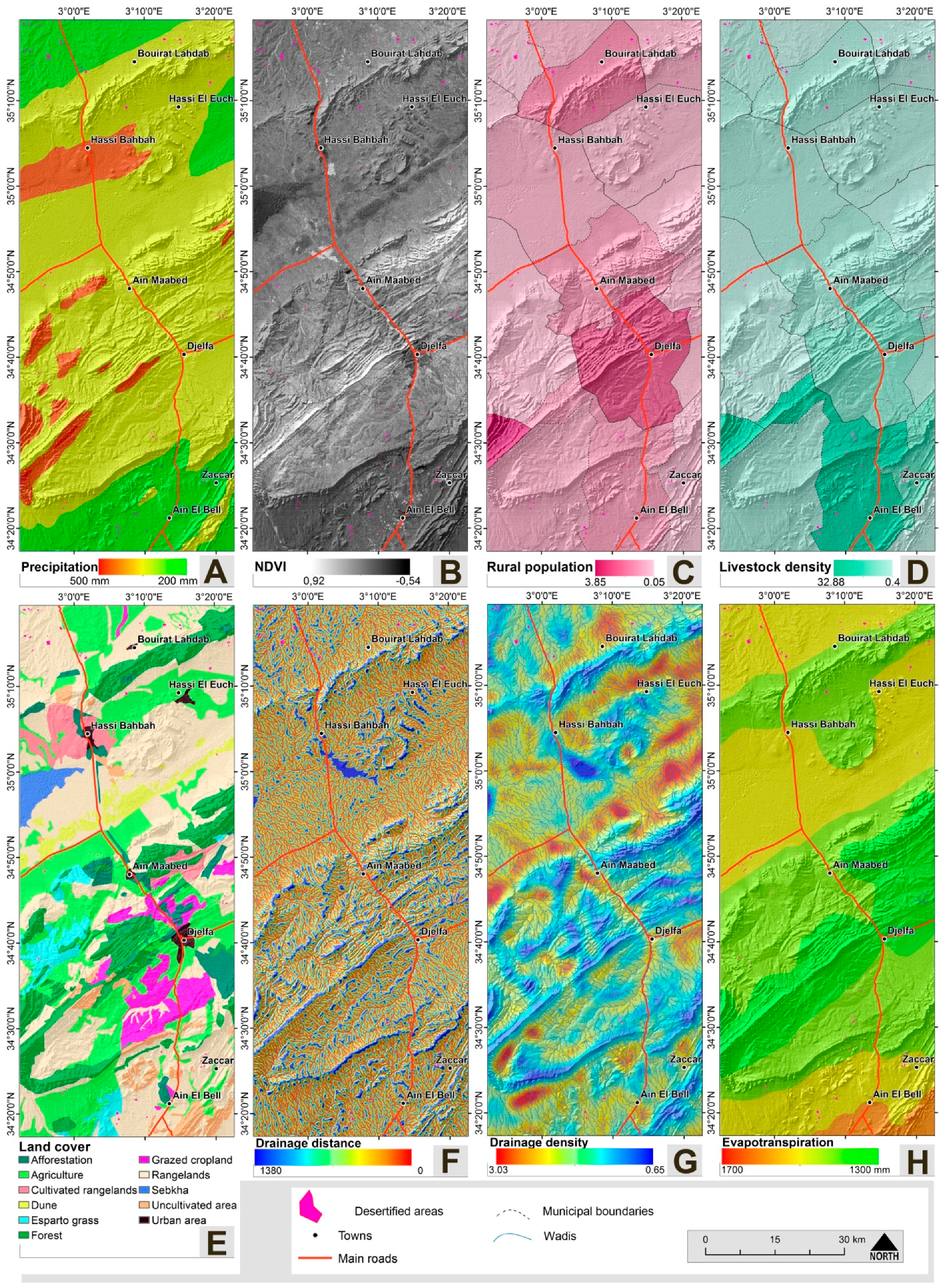
Figure 3.
Maps of the geomorphological and soil prediction factors: (A) land surface temperature (LST); (B) elevation; (C) hypsometric integral (HI); (D) curvature; (E) lithology; (F) slope; (G) topographic position index (TPI); and (H) aspect.
Figure 3.
Maps of the geomorphological and soil prediction factors: (A) land surface temperature (LST); (B) elevation; (C) hypsometric integral (HI); (D) curvature; (E) lithology; (F) slope; (G) topographic position index (TPI); and (H) aspect.

Figure 4.
The predictive factors retained in the final logistic model and their odds ratios.

Figure 5.
Desertification susceptibility map generated using a logistic model in the Djelfa area.

Figure 6.
(A) Receiver operating characteristic (ROC) curve for the logistic model; (B) sensitivity analysis with validation dataset for 50 desertification susceptibility estimates; and (C) desertification susceptibility model error. The x-axis shows the mean value of 50 probability estimates; the y-axis represents two standard deviations of the probability estimate.
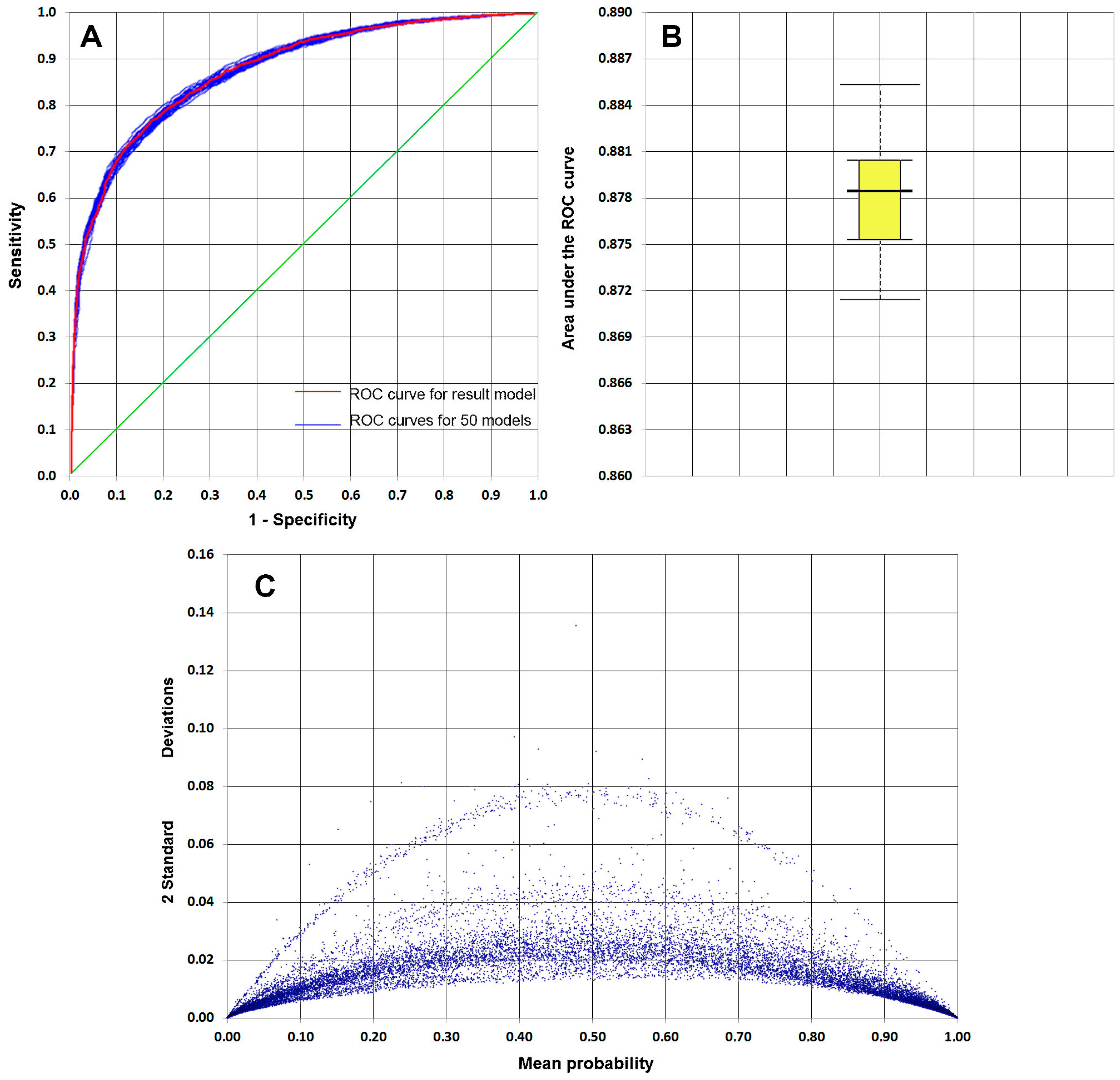

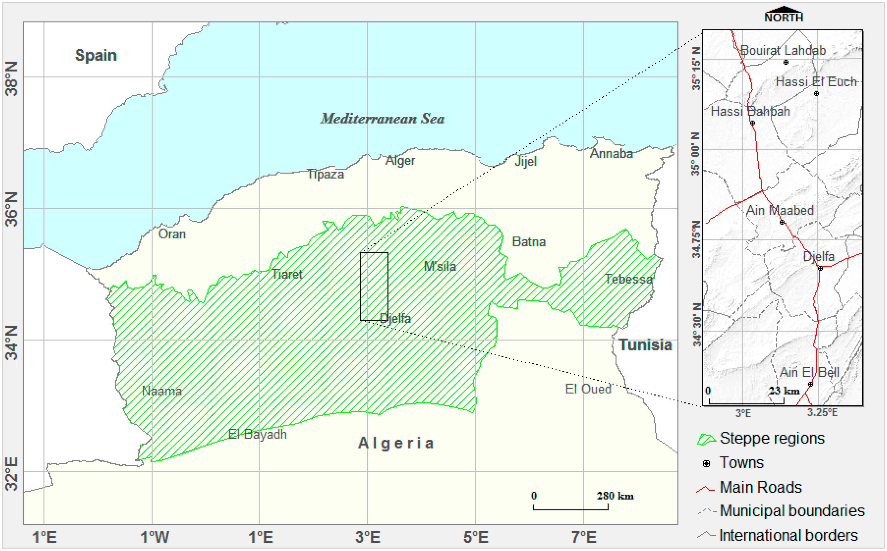
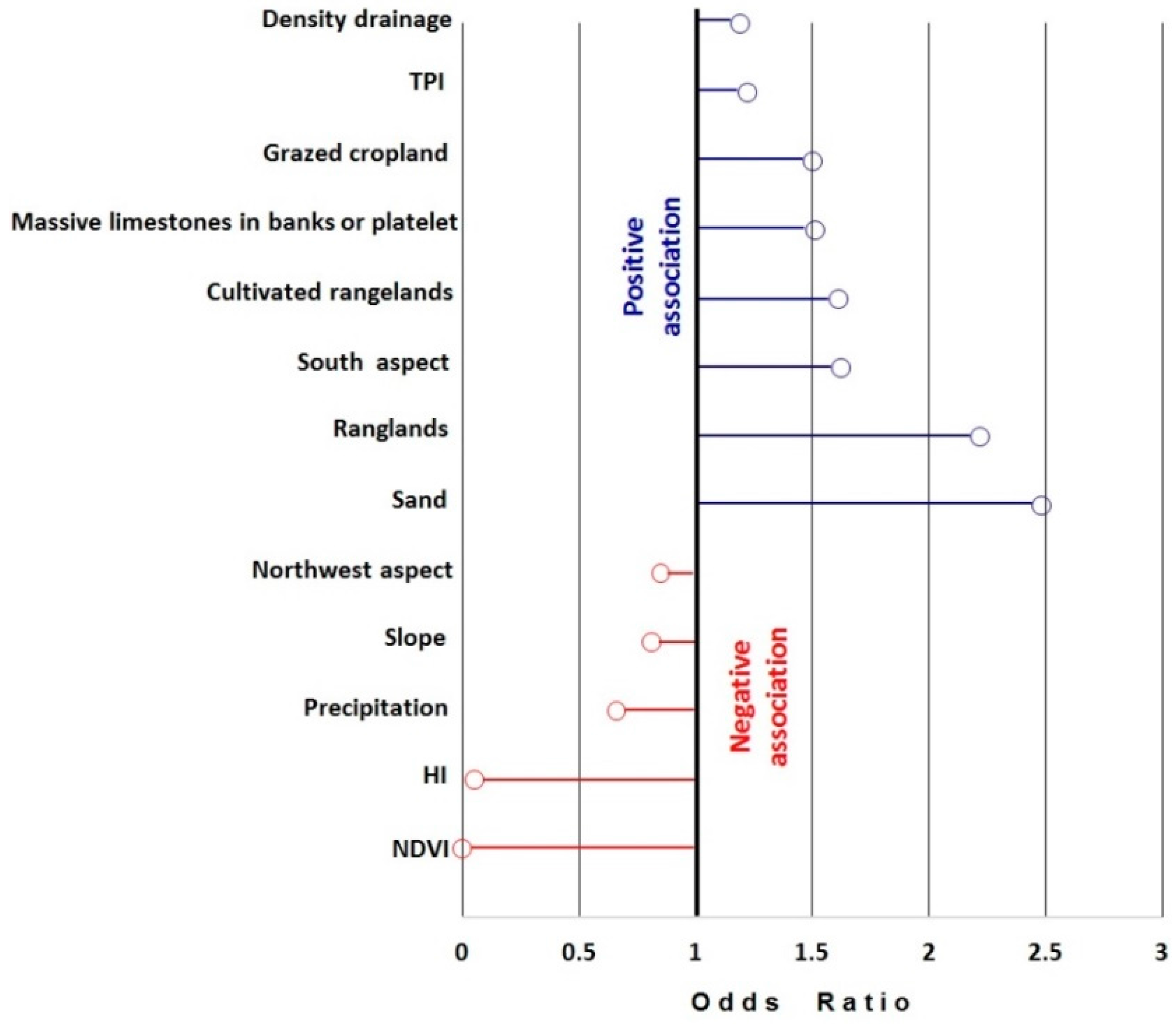
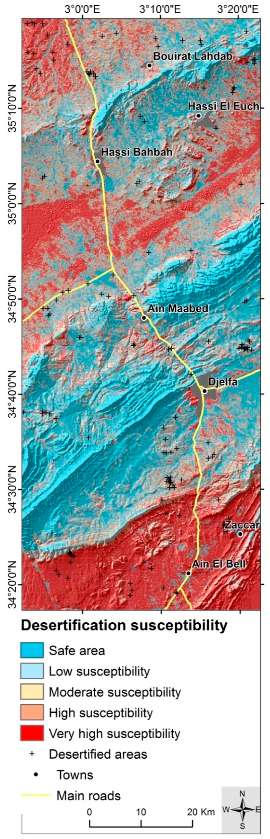
Table 1.
Evaluation of the relationships between the desertified area, represented by the training and validation dataset, and desertification-predictive factors. LST: land surface temperature; TPI: topographic position index; HI: hypsometric integral; NDVI: normalized difference vegetation index.
Table 1.
Evaluation of the relationships between the desertified area, represented by the training and validation dataset, and desertification-predictive factors. LST: land surface temperature; TPI: topographic position index; HI: hypsometric integral; NDVI: normalized difference vegetation index.
| Factor | Class | Desertified (%) | Factor | Class | Desertified (%) |
|---|---|---|---|---|---|
| TPI | (−9.56)–0 | 46.33 | Land cover | Agriculture | 19.32 |
| 0–8.78 | 53.67 | Grazed cropland | 7.81 | ||
| HI | <0.35 | 0.00 | Cultivated rangelands | 0.59 | |
| 0.35–0.6 | 93.89 | Rangelands | 64.27 | ||
| >0.6 | 6.11 | Forest | 1.04 | ||
| Slope (◦) | <5 | 84.62 | Afforestation | 0.45 | |
| 5–10 | 14.28 | Esparto grass | 5.76 | ||
| >10 | 1.10 | Dune | 0.25 | ||
| Curvature (1/m) | <0 | 41.31 | Sebkha | 0 | |
| 0 | 13.31 | Uncultivated area | 0.14 | ||
| >0 | 45.38 | Urban area | 0.38 | ||
| Aspect (degree) | Flat | 2.90 | Distance to drainage (m) | <100 | 17.51 |
| N—(337.5–22.5) | 12.19 | 100–200 | 26.36 | ||
| S—(22.5–67.5) | 14.07 | 200–300 | 28.75 | ||
| W—(67.5–112.5) | 10.30 | 300–400 | 17.15 | ||
| E—(112.5–157.5) | 12.09 | 400–500 | 8.16 | ||
| NW—(157.5–202.5) | 12.18 | 500–600 | 1.91 | ||
| NE—(202.5–247.5) | 11.98 | >600 | 0.15 | ||
| SW—(247.5–292.5) | 10.17 | LST (°C) | <38 | 36.43 | |
| SE—(292.5–337.5) | 14.73 | >38 | 63.57 | ||
| Lithology | Alluvium | 27.46 | Rural population | <0.49 | 65.00 |
| Conglomeratic clay–sand formations, lacustrine and limestone | 2.13 | >0.49 | 35.00 | ||
| Livestock density | 0.48–2.88 | 20.56 | |||
| Clay | 31.40 | 2.89–9.94 | 60.34 | ||
| Schist-marls, few limestone and gypsum intercalations | 12.66 | 9.95–17 | 4.99 | ||
| >17 | 14.11 | ||||
| Massive limestones in banks or platelets | 2.75 | Evapotranspiration | 1300–1400 | 7.19 | |
| 1400–1500 | 25.76 | ||||
| Alternating sandstone and clay | 20.49 | 1500–1600 | 65.58 | ||
| Chotts | 0.00 | 1600–1700 | 1.47 | ||
| Sand | 3.12 | <300 | 43.92 | ||
| Elevation | 700–800 | 19.33 | Precipitation (mm) | 300–400 | 54.54 |
| 800–900 | 33.11 | 400–500 | 1.54 | ||
| 900–1000 | 7.51 | >500 | 0.00 | ||
| 1000–1100 | 11.22 | Drainage density (m km−2) | 1–2 | 55.31 | |
| 1100–1200 | 10.68 | 2–4 | 44.69 | ||
| 1200–1300 | 17.06 | NDVI | <0.22 | 96.21 | |
| >1300 | 1.09 | >0.22 | 3.79 |
Table 2.
The multicollinearity diagnosis index for 13 predicting factors. VIF: variance inflation factor.
Table 2.
The multicollinearity diagnosis index for 13 predicting factors. VIF: variance inflation factor.
| Category | Factor | VIF |
|---|---|---|
| Land Cover | Rangelands | 1.22 |
| Cultivated rangelands | 1.03 | |
| Grazed cropland | 1.23 | |
| Slope Aspect | South aspect | 1.04 |
| Northwest aspect | 1.07 | |
| Lithology | Sand | 1.09 |
| Massive limestones in banks or platelets | 1.04 | |
| Slope | 1.30 | |
| NDVI | 1.38 | |
| HI | 1.04 | |
| Precipitation | 1.35 | |
| Density drainage | 1.15 | |
| TPI | 1.19 | |
Table 3.
Pseudo R2 Test of the logistic model with 13 predicting factors.
| Pseudo R2 Test | Value |
|---|---|
| Cox and Snell R2 | 0.40 |
| Nagelkerke R2 | 0.53 |
Table 4.
The predictive factors retained in the final logistic model and their estimated coefficients.
Table 4.
The predictive factors retained in the final logistic model and their estimated coefficients.
| Category | Factor | βi | Standard Error of Estimate | Wald χ2 Values | Significance (p Value) | Exp (βi) (Odds Ratio) |
|---|---|---|---|---|---|---|
| Land cover | Rangelands | 0.800 | 0.054 | 14.805 | 0.000 | 2.22 |
| Cultivated rangelands | 0.473 | 0.238 | 1.986 | 0.047 | 1.61 | |
| Grazed cropland | 0.405 | 0.088 | 4.628 | 0.000 | 1.50 | |
| Slope aspect | South aspect | 0.481 | 0.084 | 5.663 | 0.000 | 1.62 |
| Northwest aspect | −0.166 | 0.068 | −2.462 | 0.014 | 0.85 | |
| Lithology | Sand | 0.909 | 0.138 | 6.583 | 0.000 | 2.48 |
| Massive limestones in banks or platelets | 0.412 | 0.168 | 2.448 | 0.014 | 1.51 | |
| Slope | −0.209 | 0.009 | −22.617 | 0.000 | 0.81 | |
| NDVI | −52.391 | 1.270 | −41.242 | 0.000 | ~0 | |
| HI | −2.982 | 0.373 | −8.006 | 0.000 | 0.05 | |
| Precipitation | −0.420 | 0.054 | −7.763 | 0.000 | 0.66 | |
| Density drainage | 0.176 | 0.073 | 2.416 | 0.016 | 1.19 | |
| TPI | 0.198 | 0.016 | 12.263 | 0.000 | 1.22 | |
Table 5.
Classification of desertification susceptibility map into five classes.
| Susceptibility Class | Range | Number of Pixels | Area Covered (%) |
|---|---|---|---|
| Safe area | 0–0.14 | 1,325,603 | 23.99 |
| Low susceptibility | 0.15–0.36 | 930,010 | 16.83 |
| Moderate susceptibility | 0.37–0.60 | 807,834 | 14.62 |
| High susceptibility | 0.61–0.83 | 848,277 | 15.35 |
| Very-high susceptibility | 0.84–1 | 1,614,946 | 29.22 |
© 2017 by the authors. Licensee MDPI, Basel, Switzerland. This article is an open access article distributed under the terms and conditions of the Creative Commons Attribution (CC BY) license (http://creativecommons.org/licenses/by/4.0/).
Share and Cite
MDPI and ACS Style
Djeddaoui, F.; Chadli, M.; Gloaguen, R. Desertification Susceptibility Mapping Using Logistic Regression Analysis in the Djelfa Area, Algeria. Remote Sens. 2017, 9, 1031. https://doi.org/10.3390/rs9101031
AMA Style
Djeddaoui F, Chadli M, Gloaguen R. Desertification Susceptibility Mapping Using Logistic Regression Analysis in the Djelfa Area, Algeria. Remote Sensing. 2017; 9(10):1031. https://doi.org/10.3390/rs9101031
Chicago/Turabian StyleDjeddaoui, Farid, Mohammed Chadli, and Richard Gloaguen. 2017. "Desertification Susceptibility Mapping Using Logistic Regression Analysis in the Djelfa Area, Algeria" Remote Sensing 9, no. 10: 1031. https://doi.org/10.3390/rs9101031
Note that from the first issue of 2016, this journal uses article numbers instead of page numbers. See further details here.